Homotopy Theory of Finite Topological Spaces

Emily Clader

Senior Thesis

Advisor: Robert Lipshitz

Contents

Chapter 1. Introduction 5

Chapter 2. Preliminaries 71. Weak Homotopy Equivalences 72. Quasifibrations 83. The Dold-Thom Theorem 94. Inverse Limits of Topological Spaces 11

Chapter 3. The Results of McCord 15

Chapter 4. Inverse Limits of Finite Topological Spaces: An Extension of McCord 23

Chapter 5. Conclusion: Symmetric Products of Finite Topological Spaces 29

Bibliography 31

3

CHAPTER 1

Introduction

In writing about finite topological spaces, one feels the need, as McCord did in his paper“Singular Homology Groups and Homotopy Groups of Finite Topological Spaces” [8], to beginwith something of a disclaimer, a repudiation of a possible initial fear. What might occur asthe homotopy groups of a topological space with only finitely many points? The naive answerwould be to assume that these groups must be trivial. This is based, however, on a mistakenintuition, namely that a finite space is endowed with the discrete topology (as it would be,for example, if it were a finite subset of Euclidean space with the subspace topology). Upon amoment’s further reflection, however, it is apparent that this is by no means necessarily the case,and there could be many nontrivial continuous maps into finite spaces with more interestingtopologies. Indeed, the main theorem of McCord’s paper provides a correspondence up to weakhomotopy equivalence between finite topological spaces and finite simplicial complexes, provingthat these two classes of spaces exhibit precisely the same homotopy groups.

The goal of this paper is to provide a thorough explication of McCord’s results and prove anew extension of his main theorem. More specifically, Chapter Two contains the preliminarymaterial on homotopy theory, beginning with a discussion of weak homotopy equivalence andthe related notion of quasifibration. It also includes a sketch of the proof of the Dold-Thomtheorem, perhaps the most remarkable application of quasifibrations, and it concludes with abrief introduction to inverse limits of topological spaces, the main ingredient in the generalizationof McCord’s theorem presented in Chapter Four.

McCord’s paper is discussed in detail in Chapter Three. This chapter begins by establishingan equivalence between transitive, reflexive relations on a set and topologies under which theset is an A-space (that is, under which arbitrary intersections of open sets are open). Thiscorrespondence is used to prove that there is a natural association of a simplicial complex K(X)to each T0 A-space X and a weak homotopy equivalence |K(X)| → X. With the help of oneadditional theorem, this implies that every finite topological space is weakly homotopy equivalentto a finite simplicial complex. Finally, by imposing a partial order on the set of barycenters ofsimplices of a simplicial complex, the same ideas are used to prove, conversely, that every finitesimplicial complex is weakly homotopy equivalent to a finite topological space.

In Chapter Four, we prove that every finite simplicial complex is homotopy equivalent to aninverse limit of finite topological spaces, a generalization of McCord’s theorem. The idea of theproof is to associate a sequence of progressively better finite approximations to a simplicial com-plex K; the first finite approximation is the space appearing in McCord’s correspondence, whilethe rest are finite spaces with a strictly greater number of points but which retain the propertyof weak homotopy equivalence to K. By visualizing points in the inverse limit as convergentsequences of points in K, we obtain a homeomorphism between the geometric realization of Kand a quotient space of the inverse limit. Finally, we prove that this quotient space is in fact adeformation retract of the entire inverse limit, thereby obtaining the result.

5

CHAPTER 2

Preliminaries

1. Weak Homotopy Equivalences

A map f : X → Y is called a weak homotopy equivalence if the induced maps

f∗ : πn(X, x0)→ πn(Y, f(x0))

are isomorphisms for all n ≥ 0 and all basepoints x0 ∈ X. In the case where n = 0, theterm “isomorphism” should be understood as simply “bijection”, since there is no natural groupstructure on the sets π0(X, x0) and π0(Y, f(x0)), which are the sets of path-components of Xand Y respectively.

It should be noted that, as the terminology indicates, every homotopy equivalence is alsoa weak homotopy equivalence. This is obvious if we take a restricted notion of homotopyequivalence, considering only maps f : X → Y for which there exists a map g : Y → X andbased homotopies f ◦ g ∼ idY and g ◦ f ∼ idX . For in this case, the existence of these basedhomotopies together with the functoriality of πn implies that f∗◦g∗ = id and g∗◦f∗ = id, so thatf∗ and g∗ are inverse isomorphisms. But indeed, even if homotopies are not required to keepbasepoints stationary, it is true that a homotopy equivalence is a weak homotopy equivalence.The proof is a straightforward generalization of Proposition 1.18 of [6], in which the statementis proved in the special case of π1.

The converse, on the other hand, is not true: a weak homotopy equivalence is not necessarilya homotopy equivalence. Indeed, there are weak homotopy equivalences X → Y for which theredoes not exist a weak homotopy equivalence Y → X, a phenomenon which is by definitionimpossible for the stronger notion of homotopy equivalence. One such example comes fromthe so-called “real line with two origins”, the quotient space Y of R × {0, 1} obtained via theidentification (x, 0) ∼ (x, 1) if x 6= 0. There is a weak homotopy equivalence f : S1 → Y , soin particular Y has nontrivial fundamental group. However, since S1 is Hausdorff, any mapg : Y → S1 must agree on the two origins, and hence g factors through the map Y → R whichidentifies the two origins. By composing with a contraction of R we see that g is nulhomotopicand hence induces the trivial homomorphism on all homotopy groups, so it cannot be a weakhomotopy equivalence.

There is one situation, though, in which a weak homotopy equivalence is indeed a homotopyequivalence; namely, Whitehead’s theorem states that if X and Y are CW complexes andf : X → Y is a weak homotopy equivalence, then f is a homotopy equivalence. Nevertheless,most of the weak homotopy equivalences that will be considered in this paper will be mapsK → X where K is a CW complex and X is a finite topological space, so Whitehead’s Theoremwill not apply. Such maps will in general not be homotopy equivalences.

Indeed, a map from a CW complex K into a finite space X cannot be a homotopy equivalenceunless K is a disjoint union of contractible spaces. To see this, consider first the case where

7

K is connected. If a map f : K → X is a homotopy equivalence, then there exists an inversehomotopy equivalence g : X → K. The image of g ◦ f is a finite, connected subspace of K,and hence is a point. So, since g ◦ f ∼ idK , this homotopy provides a contraction of K. In thegeneral case when K is not necessarily connected, the same reasoning shows that each connectedcomponent of K must be contractible.

2. Quasifibrations

A related notion to that of weak homotopy equivalence is the notion of a quasifibration. Amap p : E → B over a path-connected base is said to be a quasifibration if the induced map

p∗ : πn(E, p−1(b), x0)→ πn(B, b)

is an isomorphism for all b ∈ B, all x0 ∈ p−1(b), and all n ≥ 0.First, as before, let us verify the logic of the terminology by observing that a fibration is also

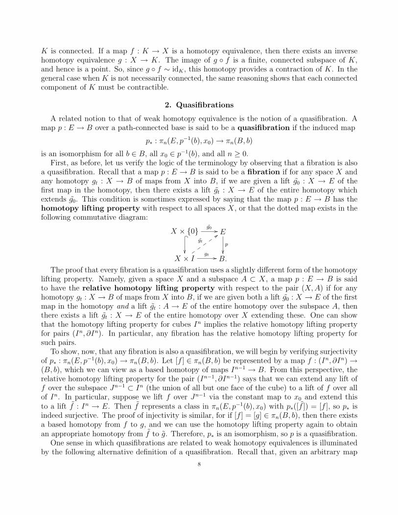
a quasifibration. Recall that a map p : E → B is said to be a fibration if for any space X andany homotopy gt : X → B of maps from X into B, if we are given a lift g0 : X → E of thefirst map in the homotopy, then there exists a lift gt : X → E of the entire homotopy whichextends g0. This condition is sometimes expressed by saying that the map p : E → B has thehomotopy lifting property with respect to all spaces X, or that the dotted map exists in thefollowing commutative diagram:

X × {0} g0 //� _

��

E

p

��X × I

gt //

gt

::vv

vv

vB.

The proof that every fibration is a quasifibration uses a slightly different form of the homotopylifting property. Namely, given a space X and a subspace A ⊂ X, a map p : E → B is saidto have the relative homotopy lifting property with respect to the pair (X,A) if for anyhomotopy gt : X → B of maps from X into B, if we are given both a lift g0 : X → E of the firstmap in the homotopy and a lift gt : A → E of the entire homotopy over the subspace A, thenthere exists a lift gt : X → E of the entire homotopy over X extending these. One can showthat the homotopy lifting property for cubes In implies the relative homotopy lifting propertyfor pairs (In, ∂In). In particular, any fibration has the relative homotopy lifting property forsuch pairs.

To show, now, that any fibration is also a quasifibration, we will begin by verifying surjectivityof p∗ : πn(E, p−1(b), x0)→ πn(B, b). Let [f ] ∈ πn(B, b) be represented by a map f : (In, ∂In)→(B, b), which we can view as a based homotopy of maps In−1 → B. From this perspective, therelative homotopy lifting property for the pair (In−1, ∂In−1) says that we can extend any lift off over the subspace Jn−1 ⊂ In (the union of all but one face of the cube) to a lift of f over allof In. In particular, suppose we lift f over Jn−1 via the constant map to x0 and extend thisto a lift f : In → E. Then f represents a class in πn(E, p−1(b), x0) with p∗([f ]) = [f ], so p∗ isindeed surjective. The proof of injectivity is similar, for if [f ] = [g] ∈ πn(B, b), then there existsa based homotopy from f to g, and we can use the homotopy lifting property again to obtainan appropriate homotopy from f to g. Therefore, p∗ is an isomorphism, so p is a quasifibration.

One sense in which quasifibrations are related to weak homotopy equivalences is illuminatedby the following alternative definition of a quasifibration. Recall that, given an arbitrary map

8

p : E → B, we define Ep ⊂ E × Map(I, B) as the space of pairs (x, γ), where x ∈ E andγ : I → B is a path starting at p(x). This space is topologized as a subspace of E ×Map(I, B),where Map(I, B) is given the compact-open topology. The projection map Ep → B given by(x, γ) 7→ γ(1) is a fibration for any map p, and the fibers Fb of this map are called the homotopyfibers of p. There is an inclusion of each fiber p−1(b) into the homotopy fiber Fb of p over b, givenby mapping x to the pair (x, γ) where γ is the constant path at x. An alternative definitionof a quasifibration is given by requiring that each of these inclusions p−1(b) ↪→ Fb be a weakhomotopy equivalence.

To see that these two definition are equivalent, notice that since Fb → Ep → B is always afibration, the map p∗ : πn(Ep, Fb, x0) → πn(B, b) is an isomorphism for all n ≥ 0. Therefore,in the following commutative diagram, the left-hand map is an isomorphism if and only if theupper map is an isomorphism:

πn(E, p−1(b), x0) //

((QQQQQQQQQQQQπn(Ep, Fb, x0)

∼=wwooooooooooo

πn(B, b).

Now, E is homeomorphic to the subspace of Ep consisting of pairs (x, γ) where γ is a constantpath at x. Moreover, there is a deformation retraction from Ep to this subspace, given by pro-gressively shrinking the paths γ to their basepoints; in particular, Ep is homotopy equivalent toE. Therefore, the upper map in the above diagram will be an isomorphism if and only if theinclusion p−1(b) ↪→ Fb is a weak homotopy equivalence, that is if and only if the alternative def-inition of a quasifibration is fulfilled. Combining these observations, we see that the alternativedefinition is fulfilled if and only if the left-hand map in the above diagram is an isomorphism,which is precisely when p is a quasifibration by our original definition.

3. The Dold-Thom Theorem

A remarkable application of quasifibrations is given in the proof of the Dold-Thom theorem;for this reason, and because it may prove useful in the possible extension of our work discussedin the conclusion, we will state the theorem and sketch its proof here.

Given a space X, there is an action of the symmetric group Sn on the product Xn of n copiesof X given by permuting the factors. The n-fold symmetric product SPn(X) is defined asthe quotient space of Xn where we factor out this action of Sn; thus, it consists of unorderedn-tuples of points in X.

If we fix a basepoint e ∈ X, we can identify each of the products Xn with the subspace{(e, x1, . . . , xn) | xi ∈ X} of Xn+1. We thus obtain an inclusion Xn ↪→ Xn+1 for each n,and since equivalent points under the action of Sn are mapped to equivalent points, this mapdescends to an inclusion SPn(X) ↪→ SPn+1(X).

The associations X 7→ SPn(X) are functorial. That is, if f : X → Y is a basepoint-

preserving map, there is an induced map f : SPn(X) → SPn(Y ) given by [(x1, . . . , xn)] 7→[(f(x1), . . . , f(xn))], and these maps satisfy (f ◦ g) = f ◦ g and id = id. Moreover, a homotopybetween two maps X → Y induces a homotopy between the corresponding maps SPn(X) →SPn(Y ), so if X is homotopy equivalent to Y then SPn(X) is homotopy equivalent to SPn(Y ).

9

The infinite symmetric product SP (X) is defined as the increasing union

SP (X) =∞⋃n=1

SPn(X),

or in other words the direct limit of the system

SP1(X) ↪→ SP2(X) ↪→ SP3(X) ↪→ · · · ,equipped with the weak (or direct limit) topology, wherein U ⊂ SP (X) is open if and only ifU ∩ SPn(X) is open for each n ≥ 1. The association X 7→ SP (X) is still functorial; a map

f : X → Y induces a map f : SPn(X) → SPn(Y ) for each n, and the restriction of each

such f to the subspace SPn−1(X) ⊂ SPn(X) is precisely the map f : SPn−1(X) → SPn−1(Y ).

Therefore, the maps f are compatible with the direct systems defining SP (X) and SP (Y ), so

they induce a continuous map f : SP (X)→ SP (Y ). For the same reason as above, homotopicmaps X → Y induce homotopic maps SP (X)→ SP (Y ).

We are now equipped to state the theorem of Dold and Thom:

Theorem 2.1 (Dold and Thom). If X is a connected CW complex with basepoint, thenπn(SP (X)) ∼= Hn(X; Z).

The proof of this result involves showing that the association X 7→ πn(SP (X)) defines areduced homology theory on the category of basepointed CW complexes. By the functoriality ofthe associations X 7→ SP (X) and SP (X) 7→ πn(SP (X)), this candidate theory is indeed func-torial. Thus, all that remains in order to show that it defines a homology theory is verificationof the following three axioms:

(1) If f : X → Y and g : X → Y are homotopic maps between CW complexes, then theyinduce the same map πn(SP (X))→ πn(SP (Y )).

(2) For CW pairs (X,A), there is a natural long exact sequence

· · · → πn(SP (A))→ πn(SP (X))→ πn(SP (X/A))→ πn−1(SP (A))→ · · · .(3) If X =

∨αXα and iα : Xα ↪→ X are the inclusions, then the homomorphism given by

⊕α(iα)∗ : ⊕απn(SP (Xα))→ πn(SP (X)) is an isomorphism for all n ≥ 0.

The first axiom is evidently satisfied by our previous observations, since we already knowthat if f ∼ g : X → Y , then f ∼ g : SP (X) → SP (Y ), and hence f and g induce the samemap on homotopy groups.

The wedge axiom is also essentially immediate, once we observe that if the basepoint in∨αXα and in each Xα is chosen to be the wedge point, then there is a homeomorphism

ϕ :∏α

′ SP (Xα)→ SP

(∨α

Xα

),

where∏′ denotes the ‘weak’ product, that is, the union of all the products of finitely many

factors. The homeomorphism ϕ is given by simply concatenating all of the tuples in the variousSP (Xα). We have a composition

SP (Xα)eiα−→ SP

(∨α

Xα

)ϕ−1

−−→∏α

′ SP (Xα),

10

which, under closer inspection, is simply the natural inclusion jα : SP (Xα) ↪→∏′

α SP (Xα).Now, the map

⊕αjα∗ :⊕α

πn(SP (Xα))→ πn

(∏α

′ SP (Xα)

)is an isomorphism, since a map f : Y →

∏′ SP (Xα) is the same as a collection of mapsfα : Y → SP (Xα) with the property that for every y ∈ Y , fα(y) is the basepoint for all butfinitely-many values of α. Therefore, since ⊕αjα∗ = ⊕αiα∗ ◦ϕ−1

∗ and ϕ is a homeomorphism, weconclude that ⊕αiα∗ is an isomorphism, as desired.

Thus, the real work of the theorem is in proving the existence of the long exact sequence.This is proved by showing that the map p : SP (X) → SP (X/A) induced by the quotient mapX → X/A is a quasifibration with fiber SP (A). To show that this map is a quasifibration, oneuses a number of locality properties of quasifibrations, first reducing the problem to showingby induction that p is a quasifibration over each subspace SPn(X/A) ⊂ SP (X/A), and thenreducing the inductive step of this latter claim to showing that if p is a quasifibration overSPn−1(X/A) then it is in fact a quasifibration over a neighborhood of SPn−1(X/A) and overSPn(X/A) \ SPn−1(X/A).

Once we have that p is a quasifibration, the long exact sequence of the pair (SP (X), SP (A))in homotopy yields:

πn(SP (X/A))

· · · // πn(SP (A))i∗ // πn(SP (X))

j∗ // πn(SP (X), SP (A))∂ //

p∗ ∼=

OO

πn−1(SP (A)) // · · · .

This allows us to write down an exact sequence

· · · // πn(SP (A))i∗ // πn(SP (X))

p∗◦j∗ // πn(SP (X/A)∂◦p−1∗ // πn−1(SP (A)) // · · · ,

whose form is as required and whose naturality is clear. This, therefore, completes the proofthat we have a reduced homology theory.

One can check that the coefficients of this homology theory, the groups πi(SP (Sn)), are thesame as the coefficients Hi(S

n) for ordinary homology. To do so requires explicitly proving thatSP (S2) ∼= CP∞ and using the suspension property of reduced homology theories to deducethe result for all higher values of n. Thus, we conclude that this homology theory agrees withstandard homology, which completes the proof of the theorem.

4. Inverse Limits of Topological Spaces

Given a countable sequence of spaces X0, X1, X2, . . . and continuous maps fn : Xn →Xn−1 for each n, the inverse limit of this sequence, denoted lim

←−Xn, is the set of all points

(x0, x1, x2, . . .) ∈∏∞

n=0Xn such that f(xn) = xn−1 for all n, topologized as a subspace of∏∞n=0Xn. The sequence of spaces and maps is sometimes called an inverse limit sequence, a

special case of the more general notion of an inverse system of topological spaces.It is possible, of course, that no point in the product

∏∞n=0Xn satisfies the requirements to

belong to the inverse limit, so the inverse limit of the sequence of spaces is empty. For example,

11

suppose we define a discrete space

Xn =∞⊔m=0

{xn,m}

for each n ≥ 0. Define continuous maps fn : Xn → Xn−1 by fn(xn,m) = xn−1,m+1. The pictureis the following, where the leftmost point in the row corresponding to Xi is the point xi,0:

X0 • • • • • · · ·

X1 •

AA��������•

AA��������•

AA��������•

AA��������• · · ·

X2 •

AA��������•

AA��������•

AA��������•

AA��������• · · ·

...

Figure 1: An inverse system for which the inverse limit is empty.

Suppose we attempt to construct a point (x0,j0 , x1,j1 , x2,j2 , . . .) in the inverse limit. We will be-gin with the point x0,j0 and observe that by the definition of the inverse limit, x1,j1 ∈ f−1

1 (x0, j0),which implies that x1,j1 = x1,j0−1. Similarly x2,j2 = x2,j0−2. Continuing in this way, we will findthat we can only repeat the process up to the first j0 iterations, at which point we are forcedto conclude that there is no appropriate point xi,ji for i > j0. Thus, the inverse limit of thissequence of spaces is empty.

One situation in which the inverse limit is never empty is when the spaces Xn are compactand Hausdorff (see [7]). This will not be the case in the inverse limits we consider in thispaper, but it will nevertheless be clear in the cases under consideration that the inverse limit isnonempty.

There is a natural map

λ : πi

(lim←−

Xn

)→ lim←−

πi(Xn)

given by viewing a map ϕ : Si → lim←−

Xn as a collection of maps ϕn : Si → Xn with the property

that for each x ∈ Si and each n, fn(ϕn(x)) = ϕn−1(x). It can be shown (see [6], Proposition4.67) that λ is surjective if the maps fn are fibrations, and λ is injective if the induced mapsfn∗ : πi+1(Xn)→ πi+1(Xn−1) are surjective for n sufficiently large.

An interesting consequence of this fact comes from the notion of a Postnikov tower. Givena connected CW complex X, a commutative diagram of the form shown below is said to be aPostnikov tower if the map X → Xn induces an isomorphism on πi for i ≤ n and πi(Xn) = 0for i > n. It is not difficult to construct a Postnikov tower for any connected CW complex X,and by the path-fibration construction mentioned in the previous section we can replace each ofthe maps Xn → Xn−1 by a fibration without losing the defining properties of the tower.

A Postnikov tower for a space X gives one an inverse system of progressively better homotopy-theoretic models of X. Since the maps πi(Xn+1) → πi(Xn) are isomorphisms for n sufficiently

12

...

��X3

��X2

��X //

>>}}}}}}}}

GG���������������X1

Figure 2: A Postnikov tower.

large, the result mentioned above implies that λ is an isomorphism. And since the maps πi(X)→πi(Xn) are isomorphisms for n sufficiently large, the same type of reasoning shows that thecomposition

πi(X)f∗−→ πi

(lim←−

Xn

)λ−→ lim←−

πi(Xn)

is an isomorphism, where f : X → lim←−

Xn is the natural map coming from the maps X → Xn.

This in particular implies that f∗ is a weak homotopy equivalence, so X is a CW approximationfor the inverse limit lim

←−Xn.

13

CHAPTER 3

The Results of McCord

In his 1965 paper Singular Homology Groups and Homotopy Groups of Finite TopologicalSpaces [8], McCord established a correspondence up to weak homotopy equivalence betweenfinite topological spaces and finite simplicial complexes. More precisely, he proved that to eachfinite simplicial complex K one can associate a finite topological space X (K) whose points arein one-to-one correspondence with the simplices of K, and if we topologize X (K) via the partialorder induced by inclusion of simplices, then the natural map K → X (K) is a weak homotopyequivalence. Conversely, he showed that to each finite topological space X one can associate asimplicial complex K(X) whose vertices are the points of X, and a weak homotopy equivalenceX → K(X).

Perhaps the first striking feature of this correspondence is that, as noted in the introduc-tion, it alleviates any concern that finite spaces might be topologically uninteresting objects;in particular, these results imply that the class of finite topological spaces enjoys precisely thesame homotopy groups as does the class of finite simplicial complexes. But more importantly,McCord’s findings hint at the possibility that useful information about a topological space canbe uncovered by studying its finite model. Recently, Barmak and Minian have explored thisnotion extensively. In [3] they introduced the notion of a collapse of finite spaces, which corre-sponds under McCord’s association to a simplicial collapse, and they used this construction todevelop an approach to simple homotopy theory based upon elementary moves on finite spaces.In [2] they defined a broader class of spaces, the so-called “h-regular CW complexes”, to whichMcCord’s theorems and their extensions apply. Aside from Barmak and Minian’s work, theresults of [8] were also recently used in an influential paper of Biss [4], which seeks to relatethe finite poset MacP(k, n), a combinatorial analogue of the Grassmanian, to its associatedsimplicial complex and thereby to the Grassmanian G(k, n) of k-planes in Rn.

This chapter is devoted to discussing McCord’s paper, which will serve as the foundationfor the generalization established in Chapter 4. Although we will generally restrict ourselves tofinite topological spaces, the results of [8] apply more generally to A-spaces, a slightly broaderclass. An A-space is a topological space in which the intersection of an arbitrary collection ofopen sets is open.

Clearly every finite space is an A-space, since an arbitrary intersection of open sets is neces-sarily a finite intersection. However, not every A-space is finite. For example, there is a topologyon Z+ generated by the sets of the form {m | m ≥ n} for each fixed n ≥ 1. Since the intersectionof an arbitrary collection of basis elements is another basis element, this topology makes Z+

into an A-space.The crucial observation for McCord’s correspondence is that given a set X, imposing a

topology on X that makes it into an A-space is equivalent to imposing a transitive, reflexiverelation on its elements. We discuss this equivalence below.

15

First, let X be an A-space; we will exhibit a transitive, reflexive relation on X. For eachx ∈ X, the open hull of x, denoted Ux, is defined as the intersection of all open subsets of Xcontaining x. This allows us to define a relation ≤ on X by declaring x ≤ y if x ∈ Uy. Thisis equivalent to the requirement that Ux ⊂ Uy, for it implies that every open set containing yalso contains x, so the collection of open sets containing y is a subset of the collection of opensets containing x; therefore, the intersection of the latter is contained in the intersection of theformer. This second description of ≤ makes it clear that it is a transitive, reflexive relation.

Lemma 3.1. Let X and Y be A-spaces, and let ≤ be the relation described above. Then amap f : X → Y is continuous if and only if it is order-preserving, that is, if and only if x ≤ yimplies f(x) ≤ f(y).

Proof. Suppose f : X → Y is continuous, and let x, y ∈ X be such that x ≤ y. Thenx ∈ Uy, and we must show that f(x) ∈ Uf(y). To do so, let V ⊂ Y be an open set containingf(y). Then f−1(V ) is an open subset of X containing y, and hence x ∈ f−1(V ). Therefore, wehave f(x) ∈ V , so that f(x) lies in every open set containing f(y). That is, f(x) ∈ Uf(y), asrequired.

Conversely, suppose f : X → Y is order-preserving, and let V ⊂ X be open. To showthat f−1(V ) ⊂ Y is open, it suffices to prove that for all y ∈ f−1(V ), Uy ⊂ f−1(V ). So, lety ∈ f−1(V ), and let x ∈ Uy. Then by definition, x ≤ y, and since f is order-preserving thisimplies that f(x) ≤ f(y), that is, f(x) lies in every open set containing f(y). In particular, Vis an open set containing f(y), so f(x) ∈ V . Therefore, x ∈ f−1(V ). We have therefore shownthat Uy ⊂ f−1(V ) for each y ∈ f−1(V ), and hence f−1(V ) is open. �

Another useful observation about the relation ≤ is that it is antisymmetric (and hence apartial order) if and only if X is T0. (Recall that a topological space X is said to be T0 if, givenany pair of distinct points in X, there exists an open set containing one but not the other.)

For the opposite direction of the equivalence between A-space structures and transitive, re-flexive relations, suppose that we are given a set X with a transitive, reflexive relation ≤. Thenwe can define, for each x ∈ X, the set Ux = {y ∈ X | y ≤ x}. This collection of sets forms thebasis for a topology on X, with the reflexivity and transitivity corresponding precisely to thetwo axioms required to be a basis. And under this topology, X is an A-space; indeed, if {Vα}α∈Ais a collection of open subsets of X and V = ∩α∈AVα, then for all x ∈ V we have x ∈ Ux ⊂ Vαfor each α, so that x ∈ Ux ⊂ V and hence V is open.

Moreover, as the notation would suggest, Ux is the open hull of x in the topology we havedefined on X. Since Ux is open by definition, it is clear that the open hull of x is contained inUx. For the reverse inclusion, let V be any open set containing x. Then we can express V as aunion of basis elements, say V = ∪z∈BUz. Since x ∈ V , x lies in some Uz, and therefore x ≤ z.Therefore, for any y ∈ Ux we have y ≤ x ≤ z, so y ∈ Uz and hence y ∈ V . This shows thatUx ⊂ V , and thus establishes that Ux is contained in every open set that contains x. Hence, Uxis exactly the open hull of x, as claimed.

With this equivalence defined, we are prepared to prove the first direction of the correspon-dence between finite topological spaces (or, more generally, A-spaces) and simplicial complexes.This is encapsulated in the following theorem:

Theorem 3.2 (McCord). There exists a correspondence that assigns to each T0 A-space X asimplicial complex K(X), whose vertices are the points of X, and a weak homotopy equivalence

16

fX : |K(X)| → X. This correspondence is natural in X: a map ϕ : X → Y of T0 A-spacesinduces a simplicial map K(X)→ K(Y ), and ϕ ◦ fX = fY ◦ |ϕ|.

To prove Theorem 3.2, we will use the equivalence discussed above to notice that since X isa T0 A-space, there is a partial order ≤ on the elements of X. With this in mind, define thesimplicial complex K(X) by letting its vertices be the points of X and its simplices be the finitesubsets of X that are totally ordered by ≤.

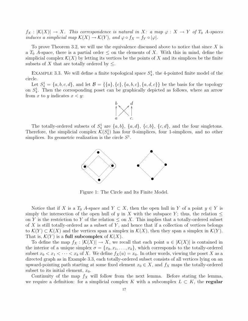
Example 3.3. We will define a finite topological space S14 , the 4-pointed finite model of the

circle.Let S1

4 = {a, b, c, d}, and let B = {{a}, {c}, {a, b, c}, {a, d, c}} be the basis for the topologyon S1

4 . Then the corresponding poset can be graphically depicted as follows, where an arrowfrom x to y indicates x < y:

b d

a

OO ??��������c.

OO__????????

The totally-ordered subsets of S14 are {a, b}, {a, d}, {c, b}, {c, d}, and the four singletons.

Therefore, the simplicial complex K(S14) has four 0-simplices, four 1-simplices, and no other

simplices. Its geometric realization is the circle S1.

Figure 1: The Circle and Its Finite Model.

Notice that if X is a T0 A-space and Y ⊂ X, then the open hull in Y of a point y ∈ Y issimply the intersection of the open hull of y in X with the subspace Y ; thus, the relation ≤on Y is the restriction to Y of the relation ≤ on X. This implies that a totally-ordered subsetof X is still totally-ordered as a subset of Y , and hence that if a collection of vertices belongsto K(Y ) ⊂ K(X) and the vertices span a simplex in K(X), then they span a simplex in K(Y ).That is, K(Y ) is a full subcomplex of K(X).

To define the map fX : |K(X)| → X, we recall that each point u ∈ |K(X)| is contained inthe interior of a unique simplex σ = {x0, x1, . . . , xk}, which corresponds to the totally-orderedsubset x0 < x1 < · · · < xk of X. We define fX(u) = x0. In other words, viewing the poset X as adirected graph as in Example 3.3, each totally-ordered subset consists of all vertices lying on anupward-pointing path starting at some fixed element x0 ∈ X, and fX maps the totally-orderedsubset to its initial element, x0.

Continuity of the map fX will follow from the next lemma. Before stating the lemma,we require a definition: for a simplicial complex K with a subcomplex L ⊂ K, the regular

17

neighborhood of L in K is the set ⋃x∈L

stK(x) ⊂ |K|,

where stK(x) denotes the open star of x in K, that is, the union of the interiors of the simplicesof K that contain x as a vertex.

Lemma 3.4. Let X be a T0 A-space, and let Y ⊂ X be open. Then (fX)−1(Y ) is the regularneighborhood of K(Y ) in K(X).

Proof. Before proving the lemma, let us observe that since regular neighborhoods arealways open, this implies that fX is continuous.

Let u ∈ (fX)−1(Y ). Then fX(u) ∈ Y , that is, u lies in the interior of a simplex σ ={x0, x1, . . . , xk} such that x0 < x1 < · · · < xk, and x0 ∈ Y . The interior of σ is therefore asubset of stK(X)(x0), so we have

u ∈ stK(X)(x0) ⊂⋃

y∈K(Y )

stK(X)(y),

that is, u lies in the regular neighborhood of K(Y ) in K(X).Conversely, suppose that u lies in the regular neighborhood of K(Y ) in K(X). Then u ∈

stK(X)(y) for some y ∈ K(Y ), and since the vertices of K(Y ) are points in Y , we can view y aslying in Y . In particular, there is a simplex σ = {x0, x1, . . . , xk} such that x0 < x1 < · · · < xk,xi = y for some i, and u ∈ int(σ). Then x0 ≤ y, so x0 ∈ Uy, which says that x0 is contained inevery open set containing y. Thus, x0 ∈ Y , which proves that fX maps the interior of σ to Y ,so fX(u) ∈ Y . We conclude that u ∈ f−1

X (Y ), as desired. �

At this point, let us digress to state (without proof) a theorem that will be used to showthat the map fX is a weak homotopy equivalence. This result appears in [8] as Theorem 6,and in [6] as Corollary 4K.2. The proof in [8] is essentially a sketch, since it closely follows theproof of an analogous result for quasifibrations (rather than weak homotopy equivalences) thatappears in [5]. The main idea behind McCord’s adaptation of the result for quasifibrations tothe present situation is the observation that a surjective map p : E → B with the propertythat πn(p−1(x), y) = 0 for all x ∈ E, y ∈ p−1(x), and n ≥ 0 is a quasifibration if and only ifit is a weak homotopy equivalence. This follows immediately from the long exact sequence inhomotopy of the pair (E, p−1(x)).

Theorem 3.5 (McCord). Let p : E → B be any continuous map, and suppose that thereexists an open cover U of B with the property that if x ∈ U ∩ V for some U, V ∈ U , then thereexists W ∈ U such that x ∈ W ⊂ U ∩ V . Suppose further that for each U ∈ U , the restrictionp|p−1(U) : p−1(U) → U is a weak homotopy equivalence. Then p is itself a weak homotopyequivalence.

In our application of this result, we will take as the open cover U the collection of sets Ux forx ∈ X. In light of this theorem, we must show that (fX)|(fX)−1(Ux) : (fX)−1(Ux)→ Ux is a weakhomotopy equivalence for all x ∈ X. We will do so by proving that its domain and codomain areboth contractible, so that the induced homomorphisms on homotopy groups are maps betweentrivial groups and hence clearly isomorphisms.

Lemma 3.6. If X is an A-space and x ∈ X, then Ux is contractible.

18

Proof. Define a homotopy F : Ux × I → Ux by

F (y, t) =

{y t ∈ [0, 1)

x t = 1.

If continuous, this clearly defines a contraction of Ux to x.To see that F is continuous, let V ⊂ Ux be open. If x ∈ V , then since no proper open subset

of Ux contains x, we must have Ux = V and hence F−1(V ) = Ux × I, which is open. If x /∈ V ,then F−1(V ) = V × [0, 1), which is also open. This completes the proof. �

Lemma 3.7. If X is a T0 A-space and x ∈ X, then (fX)−1(Ux) is contractible.

Proof. Recall that the regular neighborhood of a full subcomplex deformation retracts ontothe full subcomplex; in particular, (fX)−1(Ux) deformation retracts onto |K(Ux)|. So to provethe claim, it suffices to show that |K(Ux)| is contractible.

Let Vx = Ux \ {x}. We claim that K(Ux) = cone(K(Vx), x), or in other words that thesimplices of K(Ux) consist precisely of the simplices of K(Vx), together with simplices of theform {x0, x1, . . . , xk, x} where {x0, x1, . . . , xk} is a simplex of K(Vx).

First, any such simplex is a simplex of K(Ux). To see this, observe that every simplex of K(Vx)is of the form {x0, x1, . . . , xk} where x0 < x1 < · · · < xk, and where xi < x for all i ∈ {0, . . . , k}.Therefore, for any simplex of K(Vx), the set {x1, . . . , xk, x} is a simplex of K(Ux).

Moreover, these are all the simplices of K(Ux). For if σ = {x0, x1, . . . , xk} is a simplex ofK(Ux) but not a simplex of K(Vx), then xi = x for some i.

Thus, we have established that K(Ux) = cone(K(Vx), x), and therefore its geometric realiza-tion is contractible to the cone point x. �

The proof of Theorem 3.2 is now almost immediate:

Proof of Theorem 3.2. By the above two lemmas, the maps

(fX)|(fX)−1(Ux) : (fX)−1(Ux)→ Ux

are weak homotopy equivalences for all x ∈ X, and hence, by Theorem 3.5, fX is itself a weakhomotopy equivalence.

All that remains is to establish naturality of the association X 7→ K(X). Let ϕ : X → Y bea map of T0 A-spaces. Recall that since ϕ is continuous, it is order-preserving by Lemma 3.1.Thus, it maps totally-ordered sets onto totally-ordered sets, and so it maps simplices of K(X)onto simplices of K(Y ). That is, the map ϕ : K(X)→ K(Y ) is simplicial.

To see that ϕ ◦ fX = fY ◦ |ϕ|, let u ∈ |K(X)| lie in the interior of the simplex {x0, x1, . . . xk},where x0 < x1 < · · · < xk. Then, since ϕ is simplicial, |ϕ|(u) lies in the interior of the simplex{ϕ(x0), ϕ(x1), . . . , ϕ(xk)}, and since ϕ is order-preserving we have ϕ(x0) ≤ ϕ(x1) ≤ · · · ≤ ϕ(xk).Hence, (fY ◦|ϕ|)(u) = ϕ(x0). On the other hand, since fX(u) = x0, we have (ϕ◦fX)(u) = ϕ(x0).So fY ◦ |ϕ| = ϕ ◦ fX , as claimed. �

It should be noted that Theorem 3.2 implies that every finite T0 space is weakly homotopyequivalent to a finite simplicial complex. For the more general statement that every finite space(not necessarily T0) is weakly homotopy equivalent to a finite simplicial complex, a further resultis required:

19

Theorem 3.8 (McCord). There exists a correspondence that assigns to each A-space X a

quotient space X of X such that

(1) The quotient map νX : X → X is a homotopy equivalence,

(2) X is a T0 A-space,(3) The construction is natural in X: for each map ϕ : X → Y , there exists a unique map

ϕ : X → Y such that νY ◦ ϕ = ϕ ◦ νX .

Proof. Let X be an A-space. Define an equivalence relation ∼ on X by declaring x ∼ y ifUx = Uy, and let X = X/ ∼. Since this is equivalent to the requirement that x ≤ y and y ≤ x,we are essentially forcing that the relation ≤ is antisymmetric. To make this rigorous, though,we need to make two observations.

First of all, X is still an A-space, under the quotient topology from the quotient map νX :X → X. For if {Uα}α∈A is a collection of open sets, then we have

ν−1X

(⋂α∈A

Uα

)=⋂α∈A

ν−1X (Uα),

and hence by the definition of the quotient topology and the fact that X is an A-space, weconclude that ∩α∈AUα is open.

Second, the relation coming from this A-space structure on X is the same as the one inducedvia νX by the A-space structure on X. That is, if x, y ∈ X, then νX(x) ≤ νX(y) if andonly if x ≤ y. To see this, notice first that Ux ⊂ ν−1

X (νX(Ux)). But moreover, the reversecontainment is also true; for if z ∈ ν−1

X (νX(Ux)) then νX(z) = νX(w) for some w ∈ Ux, and thusz ∈ Uz = Uw ⊂ Ux. Therefore, we have

ν−1X (νX(Ux)) = Ux.

This in particular implies that νX(Ux) is open. Next, observe that

νX(Ux) = UνX(x).

To see why this is true, note that νX(Ux) is open and contains νX(x), so UνX(x) ⊂ νX(Ux); onthe other hand, if V ⊂ X is an open set such that νX(x) ∈ V , then ν−1

X (V ) is an open setcontaining x and hence Ux ⊂ ν−1

X (V ). Therefore, νX(Ux) ⊂ V . So νX(Ux) is contained in everyopen set that contains νX(x), that is, νX(Ux) ⊂ UνX(x).

At this point, the claim that νX(x) ≤ νX(y) if and only if x ≤ y follows immediately. For ifx ≤ y, then νX(x) ≤ νX(y) by continuity of νX ; and if νX(x) ≤ νX(y), then the above impliesthat νX(x) ∈ νX(Uy), so there exists a z ∈ Uy such that νX(x) = νX(z), and hence x ≤ z ≤ y.

Now, it is clear that the relation ≤ on X is antisymmetric (in addition to reflexive and

transitive), so X is a T0 A-space. This completes the proof of part (2) of the theorem.To see that νX is a homotopy equivalence and thereby prove part (1) of the theorem, choose

any right inverse µ : X → X. While it is not a priori obvious that the map µ is continuous,continuity indeed follows because, by the above observations, µ is necessarily order-preserving.Therefore, we have νX ◦ µ = idX . To see that π = µ ◦ νX is homotopic to idX , define a mapH : X × I → X by

H(x, t) =

{x t ∈ [0, 1)

π(x) t = 1.

20

To show that H is continuous, it suffices to verify that for each point (x, s) ∈ X × I, thereexists a neighborhood of (x, s) which is mapped by F into UF (x,s). We claim that Ux × I issuch a neighborhood. To see this, notice first that (νX ◦ π)(x) = (νX ◦ µ ◦ νX)(x) = νX(x), andhence by the definiton of νX we have Uπ(x) = Ux for all x ∈ X. This implies that UF (x,s) = Ux.Take any (y, t) ∈ Ux × I. Then, if t < 1, it is clear that F (y, t) = y ∈ Ux; if t − 1, thenF (y, t) = π(y) ∈ Uπ(y) = Uy ⊂ Ux. Therefore, it is indeed the case that F (Ux×I) ⊂ Ux = UF (x,s),and by the above observations, this completes the proof that H is continuous.

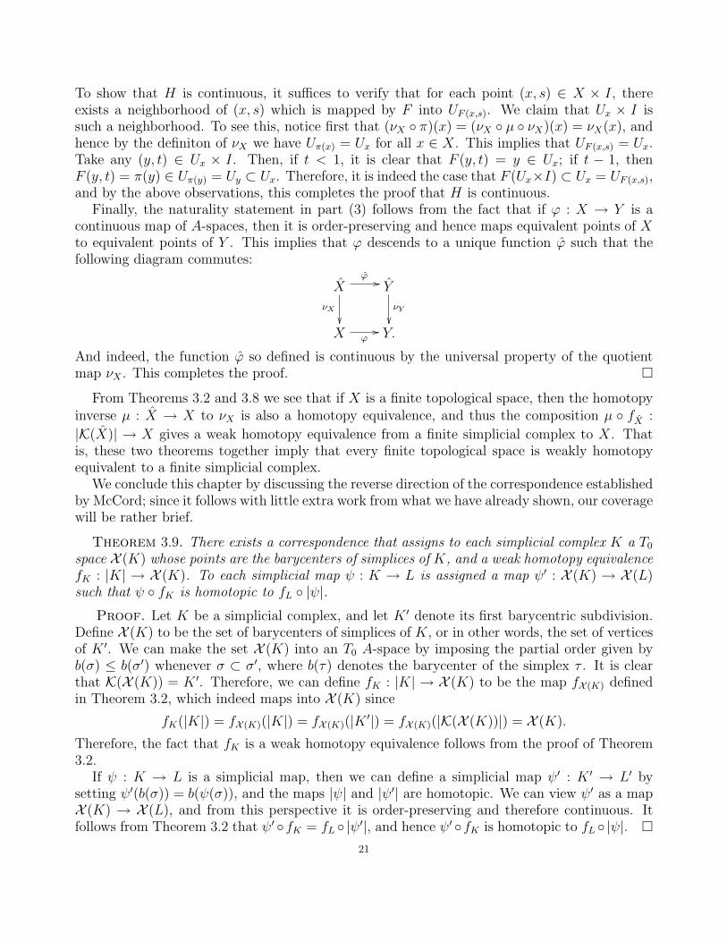
Finally, the naturality statement in part (3) follows from the fact that if ϕ : X → Y is acontinuous map of A-spaces, then it is order-preserving and hence maps equivalent points of Xto equivalent points of Y . This implies that ϕ descends to a unique function ϕ such that thefollowing diagram commutes:

Xϕ //

νX

��

Y

νY

��X ϕ

// Y.

And indeed, the function ϕ so defined is continuous by the universal property of the quotientmap νX . This completes the proof. �

From Theorems 3.2 and 3.8 we see that if X is a finite topological space, then the homotopyinverse µ : X → X to νX is also a homotopy equivalence, and thus the composition µ ◦ fX :

|K(X)| → X gives a weak homotopy equivalence from a finite simplicial complex to X. Thatis, these two theorems together imply that every finite topological space is weakly homotopyequivalent to a finite simplicial complex.

We conclude this chapter by discussing the reverse direction of the correspondence establishedby McCord; since it follows with little extra work from what we have already shown, our coveragewill be rather brief.

Theorem 3.9. There exists a correspondence that assigns to each simplicial complex K a T0

space X (K) whose points are the barycenters of simplices of K, and a weak homotopy equivalencefK : |K| → X (K). To each simplicial map ψ : K → L is assigned a map ψ′ : X (K) → X (L)such that ψ ◦ fK is homotopic to fL ◦ |ψ|.

Proof. Let K be a simplicial complex, and let K ′ denote its first barycentric subdivision.Define X (K) to be the set of barycenters of simplices of K, or in other words, the set of verticesof K ′. We can make the set X (K) into an T0 A-space by imposing the partial order given byb(σ) ≤ b(σ′) whenever σ ⊂ σ′, where b(τ) denotes the barycenter of the simplex τ . It is clearthat K(X (K)) = K ′. Therefore, we can define fK : |K| → X (K) to be the map fX (K) definedin Theorem 3.2, which indeed maps into X (K) since

fK(|K|) = fX (K)(|K|) = fX (K)(|K ′|) = fX (K)(|K(X (K))|) = X (K).

Therefore, the fact that fK is a weak homotopy equivalence follows from the proof of Theorem3.2.

If ψ : K → L is a simplicial map, then we can define a simplicial map ψ′ : K ′ → L′ bysetting ψ′(b(σ)) = b(ψ(σ)), and the maps |ψ| and |ψ′| are homotopic. We can view ψ′ as a mapX (K) → X (L), and from this perspective it is order-preserving and therefore continuous. Itfollows from Theorem 3.2 that ψ′ ◦fK = fL ◦ |ψ′|, and hence ψ′ ◦fK is homotopic to fL ◦ |ψ|. �

21

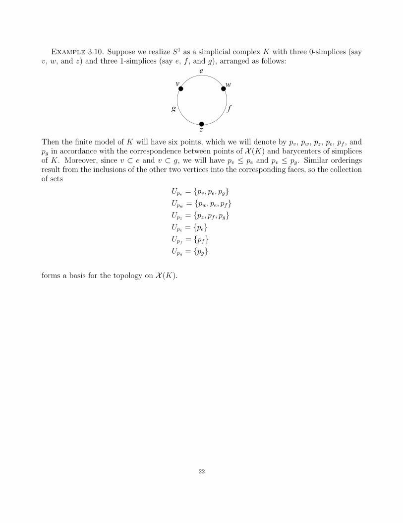
Example 3.10. Suppose we realize S1 as a simplicial complex K with three 0-simplices (sayv, w, and z) and three 1-simplices (say e, f , and g), arranged as follows:

v w

z

e

fg

Then the finite model of K will have six points, which we will denote by pv, pw, pz, pe, pf , andpg in accordance with the correspondence between points of X (K) and barycenters of simplicesof K. Moreover, since v ⊂ e and v ⊂ g, we will have pv ≤ pe and pv ≤ pg. Similar orderingsresult from the inclusions of the other two vertices into the corresponding faces, so the collectionof sets

Upv = {pv, pe, pg}Upw = {pw, pe, pf}Upz = {pz, pf , pg}Upe = {pe}Upf = {pf}Upg = {pg}

forms a basis for the topology on X (K).

22

CHAPTER 4

Inverse Limits of Finite Topological Spaces: An Extension ofMcCord

It follows from Theorem 3.9 that every finite simplicial complex K is weakly homotopyequivalent to a finite topological space X (K). The space X (K) is aptly termed the “finitemodel” of K, for it not only has isomorphic homotopy groups but, at least in the case ofExample 3.3, also bears some intuitive resemblance to the original simplicial complex. Thisinvites the question: might we model K better? Is it possible to obtain a finite topologicalspace with strictly more points than X (K), which nevertheless retains the property of weakhomotopy equivalence to K? If so, we might then wonder whether, by a process of iterativelyrefining our models, we might in the limit get the original space K back again.

These are the questions that motivate the following result:

Theorem 4.1. Any finite simplicial complex is homotopy equivalent to the inverse limit of asequence of finite spaces.

The first space in the inverse limit is essentially McCord’s space X (K), and each of theothers is indeed a larger finite space that is weakly homotopy equivalent to K. Althoughthe inverse limit of these finite spaces is not, as we might have hoped, homeomorphic to theoriginal simplicial complex, the homotopy equivalence mentioned in the theorem is in some sense“almost” a homeomorphism; it is a homeomorphism onto a quotient space of the inverse limit,and moreover onto a quotient space to which the entire inverse limit deformation retracts.

We will begin by discussing how the finite spaces are constructed.Let K be a finite simplicial complex. To construct its finite models, we begin by letting X0

be the finite space whose points are in one-to-one correspondence with the faces of simplicesof K, just as in McCord’s definition of X (K). Also analogously to McCord, we make X0 intoa poset by declaring that if x, y ∈ X0 correspond to the faces σx and σy of K, then x ≤ y ifand only if σx ⊆ σy. We topologize this finite space slightly differently than McCord’s X (K),however; in our case, we endow X0 with the topology generated by the sets

Bx = {y ∈ X0 | x ≤ y}for x ∈ X0, as opposed to the sets Ux defined in the previous section. The reason for thisdistinction involves the continuity of the maps qn defined below.

For each n ≥ 0, let Kn denote the nth barycentric subdivision of K, and let Xn be the finitespace whose points are in one-to-one correspondence with the faces of simplices of Kn. Using ananalogous partial order on the points of Xn, we can endow each Xn with the topology generatedby the sets Bx as above.

There is a natural map pn : |K| → Xn for each n, since every point in K is contained in theinterior of precisely one face of the nth barycentric subdivision of K; indeed, this is precisely themap fKn appearing in Theorem 3.9. Moreover, there is a unique projection map qn : Xn → Xn−1

23

making the following diagram commute:

|K|pn

}}|||||||| pn−1

##FFFFFFFF

Xn

qn // Xn−1.

In light of the correspondence between points in Xn and faces of simplices in Kn, we willtypically denote the simplex corresponding to x ∈ Xn by σnx . It is straightforward to check thatfor each n ≥ 0 and each x ∈ Xn, one has

p−1n (Bx) = stn(σnx),

where stn(σnx) is the open star of σnx in Kn. This implies in particular that the maps pn are allcontinuous, even in our modified topology on Xn. They are also open maps; for if U ⊂ |K| isopen and x ∈ pn(U), then there exists z ∈ U such that x = pn(z), or in other words, z ∈ int(σnx).So to say that x ∈ pn(U) is to say that int(σnx) ∩ U 6= ∅, and it is easy to see that this impliesthat for any simplex σny of Kn such that σnx ⊂ σny , we also have int(σny )∩U 6= ∅. That is, if x ≤ ythen y ∈ pn(U), so Bx ⊂ pn(U). This says that for each x ∈ pn(U) one has x ∈ Bx ⊂ pn(U),and hence pn(U) is open.

By the commutativity of the above diagram, this implies that each qn is continuous. Hence,we now have an inverse system:

X0q1←− X1

q2←− X2q3←− X3

q4←− · · ·and we can define X to be its inverse limit. The main work of the proof of Theorem 4.1 will bein showing that |K| is homeomorphic to a quotient space of X.

Before doing so, however, it should be noted that the maps pn : |K| → Xn are all stillweak homotopy equivalences. To prove this, recall that for any basis element Bx ⊂ Xn, theset p−1

n (Bx) = stn(σnx) is contractible. And, using the fact that Bx is the smallest open setcontaining x, it is readily verified that each Bx is also contractible. Hence the restrictionpn|p−1

n (Bx) : p−1n (Bx) → Bx is a weak homotopy equivalence for each basis element Bx, and by

Theorem 3.5 this is sufficient to conclude that pn is a weak homotopy equivalence.

Lemma 4.2. If K is a finite simplicial complex and the finite spaces Xn are defined as above,then |K| is homeomorphic to a quotient space of lim

←−Xn.

Proof. Given x = (x0, x1, x2, . . .) ∈ X, we can associate to x a sequence of points in |K| bychoosing an arbitrary element an ∈ p−1

n (xn) for each n ≥ 0. Because these points lie in nestedsimplices of increasingly fine barycentric subdivisions of K, and since the maximum diameterof a geometric simplex of |Kn| approaches zero as n approaches infinity, any sequence obtainedin this way is Cauchy and therefore convergent.

Now, we could have chosen a different sequence {an} corresponding to the same elementx ∈ X. However, we claim that if {an} and {bn} are any two sequences obtained in this way,then limn→∞ an = limn→∞ bn. To see this, let a = limn→∞ and let ε > 0. By the convergenceof {an}, there exists a natural number N such that |a − an| < ε

2for all n > N . And because

the diameters of the simplices p−1n (xn) approach zero as n approaches infinity, there also exists

a natural number M such that |an − bn| < ε2

for all n > M . So for n > max{N,M}, we havethat |a− bn| < ε, and hence {bn} converges to a, also.

24

We have thus established that there is a well-defined map

G : X → |K|

given by sending (x0, x1, x2, . . .) to the limit of any sequence {an} ⊂ |K| where pn(an) = xn forall n. To prove that G is continuous, let U ⊂ |K| be any open set, and let x = (x0, x1, x2, . . .) ∈G−1(U). First, observe that

G−1(U) ⊂∞∏n=0

pn(U),

that is, xn ∈ pn(U) for all n. For if there exists some n such that xn /∈ pn(U) and {an} is as above,then the commutativity of the diagram on the previous page implies that pn(an+1) /∈ pn(U) andhence an+1 /∈ U . Similarly, we obtain that ai /∈ U for all i > n, contradicting the assumptionthat the the sequence {an} converges to G(x) ∈ U . So, the above containment holds, andtherefore we may as well assume that an ∈ U for all n. Since U is open and {an} converges toa point in U , there is an open set V such that each an ∈ V and such that V ⊂ U . Now, the set

∞∏n=0

pn(V )

is open since the pn are open maps. Moreover, if y = (y0, y1, y2, . . .) ∈∏pn(V ), then yn ∈ pn(V )

for all n, so we can choose a sequence {bn} ⊂ V such that pn(bn) = yn for all n. Denote thelimit of {bn} by b, so that b = G(y). Then, since {bn} ⊂ V , we have b ∈ V ⊂ U , so y ∈ G−1(U).Thus,

x ∈∞∏n=0

pn(V ) ⊂ G−1(U),

and hence G−1(U) is open.Define an equivalence relation on X by x ∼ y if and only if G(x) = G(y), and denote by Y

the corresponding quotient space of X. (In fact, one can check that this equivalence relationis simply the T1 relation, wherein x ∼ y if and only if either every open set containing x alsocontains y or vise versa, since any open set in X containing (p0(z), p1(z), p2(z), . . .) necessarilycontains every x such that G(x) = z. Thus, we might say that Y is the “T1-ification” of X.)

We get an induced map G : Y → |K|, which is by construction both well-defined and injective.Since G([(p0(x), p1(x), p2(x), . . .)]) = x for any x ∈ |K|, it is also clearly surjective. Hence G isa bijection. It is continuous by the universal property of quotient spaces, since if π : X → Yis the quotient map then G = G ◦ π is continuous. And its inverse is the map G−1 : |K| → Ydefined by

x 7→ [(p0(x), p1(x), p2(x) . . .)],

which is the composition of the quotient map π with the map x 7→ (p0(x), p1(x), p2(x), . . .), andhence is continuous. Thus, G is a homeomorphism. �

All that remains, now, is to show that in fact Y is homotopy equivalent to |K|. This will beachieved by way of the following lemma:

Lemma 4.3. The quotient space Y is homeomorphic to a deformation retract of X.

25

Proof. Let x ∈ X, and suppose that G(x) = y. We claim that every neighborhood ofthe point (p0(y), p1(y), p2(y), . . .) ∈ X contains x. To see this, let x = (x0, x1, x2, . . .), and let{an} be a sequence of points converging to y such that pn(an) = xn for all n. Then, for eachn ≥ 0, y lies in the interior of precisely one simplex σn of Kn, and moreover, it clearly mustbe the case that an ∈ stn(σn). This implies that for each n, xn ∈ pn(stn(σn)) = Bpn(y) ⊂ Xn.But since Bpn(y) is the smallest open subset of Xn containing pn(y), this implies that any

open subset of Xn containing pn(y) also contains xn. Hence, any open subset of X containing(p0(y), p1(y), p2(y), . . .) also contains x, as claimed.

Let E be any equivalence class under ∼, wherein every element defines a sequence convergingto x ∈ |K|. Define a homotopy hE : E × [0, 1]→ hE by

hE(y, t) =

{y if t ∈ [0, 1)

(p0(x), p1(x), . . .) if t = 1.

To see that this is continuous, let U ⊂ Y be open. If the point (p0(x), p1(x), . . .) lies in U ,then every element of the equivalence class also lies in U , so that h−1

E (U) = Y × [0, 1]. If(p0(x), p1(x), . . .) /∈ U , then h−1

E (U) = U × [0, 1), which is open. Hence, hE is continuous, andso we have a homotopy from the identity map on Y to a constant map. In particular, we haveshown that every equivalence class is contractible.

Combining all of these homotopies on the various equivalence classes, we obtain a map F :X × [0, 1] → X, which we claim is also continuous. To verify this, let U ⊂ X be open, anddefine a subset UBC ⊂ U as follows:

UBC = {x ∈ U | (p0(G(x)), p1(G(x)), . . .) /∈ U}.These are the “boundary-convergent” points in U , those that we view as sequences of points inthe open set U converging to a point that is not in U . The set UBC is closed in U , since we candefine a continuous map p : X → X by p(x) = (p0(G(x)), p1(G(x)), · · · ), and

U \ UBC = {x ∈ U | p(x) ∈ U} = U ∩ p−1(U),

which is an intersection of two open sets by the continuity of p and hence is open. Moreover:

F−1(U) = (U × [0, 1]) \ (UBC × {1}),so F−1(U) is open. Therefore, F is continuous, as claimed.

We have thus defined a deformation retraction of X onto a subspace Z that contains exactlyone element from each equivalence class. It is clear that if i : Z ↪→ X is the inclusion map andπ : X → Y is the quotient map as above, then the map

f = π ◦ i : Z → Y,

is a bijection. Indeed, this map is a homeomorphism; for if U ⊂ Z is open, then U = V ∩ Z forsome open subset V ⊂ X, and π(V ) = f(U). And by the definition of Z, the set V is forcedto contain every point in each equivalence class it intersects, so π−1(π(V )) = V . In particular,π(V ) is open, so f is an open map. Conversely, if U ⊂ Y is open, then π−1(V ) ⊂ X is open, soπ−1(V ) ∩ Z = f−1(Z) is open in Z. Hence f is continuous.

Therefore, by the composition of the homotopy equivalence X → Z and the homeomorphismf : Z → Y , we obtain the claim. �

The proof of Theorem 4.1 is now immediate:

26

Proof of Theorem 4.1. Composing the homeomorphism from Lemma 4.2 and the ho-motopy equivalence from Lemma 4.3, we obtain the desired result. �

It is worth noting that, as observed by Barmak and Minian in [2], McCord’s results applymore generally to regular CW complexes. Recall that a CW complex is regular if its attachingmaps are all embeddings; it can be shown that this implies that the closure of each cell is asubcomplex. If K is a regular CW complex, one can define an associated simplicial complex K ′

whose vertices are the cells of K and whose n-simplices are the sets {e1, e2, · · · , en} of simpliceswhere ei is a face of ei+1 for each i. Moreover, |K ′| is homeomorphic to K. Therefore, thecomposition of this homeomorphism with the map fK′ : |K ′| → X (K ′) is a weak homotopyequivalence from K to a finite space.

For the same reasons, then, if K is a regular CW complex, we can apply the results ofTheorem 4.1 to the simplicial complex K ′ to show that K is homotopy equivalent to an inverselimit of finite topological spaces.

27

CHAPTER 5

Conclusion: Symmetric Products of Finite Topological Spaces

A possible extension of this work could come from studying the symmetric products of finitetopological spaces. In particular, if K is a simplicial complex, one can consider, on one hand,the spaces SPn(X (K)); on the other hand, each SPn(K) is naturally a ∆-complex (see [6]), andhence one can subdivide it to give it the structure of a simplicial complex and then considerX (SPn(K)). It seems plausible that SPn(X (K)) and X (SPn(K)) are closely related, perhapsweakly homotopy equivalent, so this topic may merit further investigation.

Moreover, the infinite symmetric product of a space is a monoid under the operation givenby concatenating tuples, and under good conditions this operation is continuous as a mapµ : SP (X)×SP (X)→ SP (X). If µ is indeed continuous, then the set of based homotopy classesof maps into SP (X) from some other basepointed topological space Y , denoted 〈Y, SP (X)〉,inherits the structure of a monoid, where we multiply maps pointwise. More generally, even if µis not necessarily continuous, the set 〈Y, SP (X)〉 still forms a monoid as long as Y is compact.For if Y is compact and f, g : Y → SP (X) are basepoint-preserving maps, then f(Y ) and g(Y )are compact subsets of SP (X) and hence they lie in finite symmetric products SPn(X) andSPm(X), respectively. In particular, (f · g)(Y ) ⊂ SPn+m(X), so if U ⊂ SP (X) is any open set,then

(f · g)−1(U) = (f · g)−1(U ∩ SPn+m(X)) = f−1(U ∩ SPn(X)) ∩ g−1(U ∩ SPm(X)),

which is the intersection of two open sets (and hence open) since both f and g are continuous.So f · g is continuous, and we can conclude that 〈Y, SP (X)〉 is a monoid.

Given these monoids, one could take their group completions 〈Y, SP (X)〉∗. It might beinteresting to check whether a cohomology theory arises in this way. For example, one coulddefine

hn(Y ) = 〈Y, SP (X (Sn))〉∗.It is not clear whether this satisfies the necessary axioms required to define a cohomology theory,or indeed, even whether 〈Y, SP (X (Sn))〉 is a monoid at all (unless, as noted above, we restrictourselves to compact spaces Y ). However, it would be interesting to explore whether this isthe case, and if so, whether the resulting cohomology theory distinguishes between topologicalspaces (perhaps finite spaces) that singular cohomology does not.

29

Bibliography

[1] M. Aguilar, S. Gitler, and C. Prieto. Algebraic topology from a homotopical viewpoint. Universitext. Springer-Verlag, New York, 2002. Translated from the Spanish by Stephen Bruce Sontz.

[2] J. A. Barmak and E. G. Minian. One-point reductions of finite spaces, h-regular CW-complexes and collapsi-bility. Algebr. Geom. Topol., 8(3):1763–1780, 2008.

[3] J. A. Barmak and E. G. Minian. Simple homotopy types and finite spaces. Adv. Math., 218(1):87–104, 2008.[4] D. K. Biss. The homotopy type of the matroid Grassmannian. Ann. of Math. (2), 158(3):929–952, 2003.[5] A. Dold and R. Thom. Quasifaserungen und unendliche symmetrische Produkte. Ann. of Math. (2), 67:239–

281, 1958.[6] A. Hatcher. Algebraic topology. Cambridge University Press, Cambridge, 2002.[7] J. G. Hocking and G. S. Young. Topology. Addison-Wesley Publishing Co., Inc., Reading, Mass.-London,

1961.[8] M. C. McCord. Singular homology groups and homotopy groups of finite topological spaces. Duke Math. J.,

33:465–474, 1966.

31