Homological Algebra over the Representation Green Functor

Homological Algebra over the Representation Green Functor

SPUR Final Paper, Summer 2012

Yajit JainMentor: John Ullman

Project suggested by: Mark Behrens

February 1, 2013

Abstract

In this paper we compute ExtRpF, F q for modules over the representation Green functor R with Fgiven to be the fixed point functor. These functors are Mackey functors, defined in terms of a specificgroup with coefficients in a commutative ring. Previous work by J. Ventura [1] computes these derivedfunctors for cyclic groups of order 2k with coefficients in F2. We give computations for general cyclicgroups with coefficients in a general field of finite characteristic as well as the symmetric group on threeelements with coefficients in F2.

1

1 IntroductionMackey functors are algebraic objects that arise in group representation theory and in equivariant stablehomotopy theory, where they arise as stable homotopy groups of equivariant spectra. However, they can begiven a purely algebraic definition (see [2]), and there are many interesting problems related to them. Inthis paper we compute derived functors Ext of the internal homomorphism functor defined on the categoryof modules over the representation Green functor R. These Mackey functors arise in Künneth spectralsequences for equivariant K-theory (see [1]). We begin by giving definitions of the Burnside category and ofMackey functors. These objects depend on a specific finite group G. It is possible to define a tensor productof Mackey functors, allowing us to identify ’rings’ in the category of Mackey functors, otherwise known asGreen functors. We can then define modules over Green functors. The category of R modules has enoughprojectives, allowing us to do homological algebra. We compute projective resolutions for the R-moduleF , the fixed point functor, and then proceed to compute ExtRpF, F q. We perform these computations forcyclic groups with coefficients in a field and for the symmetric group on three elements with coefficients inF2 using techniques derived from those used by J. Ventura in [1] to compute ExtpF, F q for the group C2k

with coefficients in F2.

2 AcknowledgementsThe work discussed in this paper was completed during the 2012 SPUR program at MIT (Summer Programin Undergraduate Research). I would like to thank the program directors Professors Pavel Etingof and SlavaGerovitch for their hard work and continued support. I would also like to thank Professor Mark Behrens forhis many edits and for suggesting the topic of this research. Finally I would like to thank John Ullman forbeing an outstanding mentor and for spending many hours patiently working with me on this project.

3 Background and Notation

3.1 Mackey FunctorsWe begin with definitions of the Burnside category and Mackey functors. For a finite group G we shalldenote the Burnside category as BG. Before defining BG it is convenient to begin with an auxiliary categoryB1G. Given a finite group G, B1G is the category whose objects are finite G-sets and morphisms from T to Sare isomorphism classes of diagrams

We define composition of morphisms to be the pullback of two diagrams:

If we define addition of morphisms asit follows that HompS, T q is a commutative monoid. This construction of B1G allows us to define BG:

Definition 3.1. Given a finite group G, the Burnside category BG is the category whose objects are the sameas the objects of B1G and for two G-sets S and T , HomBGpS, T q is the Grothendieck group of HomB1GpS, T q.

1

Given a map of G-sets f : S Ñ T , there are two corresponding morphisms in BG. The first is depicted onthe left in the figure below and is referred to as a ’forward arrow’ (denoted by f) and the second is on theright and is referred to as a ’backward arrow’ (denoted by f̂).

Definition 3.2. A Mackey functor for a group is an additive contravariant functor from the BurnsideCategory BG to the category of Abelian groups. A morphism of Mackey functors is a natural transformation.

Recall that as a consequence of additivity and functoriality we have the following:

Proposition 3.3. It is sufficient to define Mackey functors on G-sets of the form G{H for any subgroupH, quotient maps between these orbits, and conjugation maps from an orbit to an isomorphic orbit.

Definition 3.4. Denote by πHK , the quotient map from G{K to G{H where K Ă H and by γx,H theconjugation map that maps H Ñ Hx´1. Given a Mackey functor M , we refer to MpπHK q as a restrictionmap, Mpπ̂HK q as a transfer map, and Mpγx,Hq as a conjugation map. We shall denote restriction maps asrHK , transfer maps as tHK , and conjugation maps as τ .

We recall three examples of Mackey functors that we will be concerned with in this paper.

Example 3.5. We denote by R the representation functor defined by RpG{Hq “ RUpHq where RUpHq isthe complex representation ring of H. The restriction maps are restriction of representations, the transfermaps are induction of representations, and the conjugations Rpγx,Hq send a vector space with an action ofH to the same vector space where the action is redefined as h ¨ v “ xhx´1v.

Example 3.6. Let M be an abelian group with G-action. Denote the fixed point functor by FPM . ThenFPM pG{Hq “ MH . Restriction maps are inclusions of MH into MK and transfer maps send m Ñř

hPH{K hm. The conjugations are maps from MH Ñ MxH which send m Ñ xm. In this paper we only

consider the fixed point functor for G-modules M with trivial G-action. Then FPM pG{Hq “M , the restric-tions are multiplication by 1, the transfers are multiplication by the index rH : Ks, and the conjugations areidentity maps.

Example 3.7. The representable functor r´, Xs “ HomBGp´, Xq is a Mackey functor.

Definition 3.8. If M is a Mackey functor and X is a G-set, then we can define the Mackey functor MX

where

MXpY q –MpY ˆXq

for any G-set Y .

We can define a tensor product on Mackey functors such that given X,Y, Z there is a one to one correspon-dence between maps X b Y Ñ Z and natural transformations XpSq b Y pT q Ñ ZpS ˆ T q for G-sets S andT [1]. The unit for this tensor product is r´, es, the burnside ring Mackey functor Ae.

2

Definition 3.9. The internal hom functor HompX,Y q is the Mackey functor for which

HompA,HompX,Y qq – HompAbX,Y q.

There are several useful identities related to the internal hom functor. We list them here and refer to proofsin [1, 2, 4].

HompM,NqpG{Hq – HompM |H , N |HqHompM,N b r´, G{Hsq

HompM b r´, G{Hs, Nq

HomRpRX ,MqpG{Hq –MXpG{Hq –MpG{H ˆXq.

We also have the property of duality which gives us the identity

HompM,N b r´, Xsq – HompM b r´, Xs, Nq.

3.2 Green FunctorsA Green functor should be thought of as a Mackey functor with an additional ring structure where multi-plication is given by a tensor product of Mackey functors. There are two equivalent definitions of a Greenfunctor: the first reflects the previous statement and the second simplifies the task of identifying Greenfunctors and modules over Green functors.

Definition 3.10. A Green functor R for a group G is a Mackey functor for G with maps R bRÑ R andr´, es Ñ R with associative and unital properties.

Definition 3.11. A Mackey functor R is a Green functor if for any G-set S, RpSq is a ring, restrictionmaps are ring homomorphisms that preserve the unit, and the following Frobenius relations are satisfied forall subgroups K Ă H of G with a P RpKq and b P RpHq:

bptHKaq “ tHKpprHKbqaq

ptHKaqb “ tHKpaprHKbqq

Definition 3.12. Given a Green functor R, a Mackey functor M is an R-module if for a G-set S, MpSq isan RpSq-module, and for a G-map f : S Ñ T the following are true [1]:

Mpfqpamq “ RpfqpaqMpfqpmq @ a P RpY q,m PMpY q

aMpf̂qpmq “Mpf̂qpRpfqpaqmq @ a P RpY q,m PMpXq

Rpfqpaqm “Mpf̂qpaMpf̂qpmqq @ a P RpXq,m PMpY q

Definition 3.13. A morphism f of R-modules is a morphism of Mackey functors that preserves the actionof R.

Example 3.14. The representation functor R is a Green functor.

Example 3.15. The fixed point functor is an R-module where R is the representation functor. The actionof R on F is given by the augmentation map σ ÞÑ dimpσq for a representation σ.

Example 3.16. The functor RG{e – Rb r´, G{es is an R-module.

This setup allows us to compute the homology of modules over Green functors.

3

4 Computation for G “ Cn

From this point onward we will let R denote RbK for a fixed field K. Simlarly, F will denote FPK for thetrivial G-module K. We intend to compute the derived functors ExtRpF, F q for the group G “ Cn.

There are three steps to computing ExtRpF, F q. We first compute a projective resolution of F . Next wemust apply the functor HomRp´, F q to this projective resolution. We then compute the homology groupsof the resulting chain complex to get ExtRpF, F q. One additional computation gives us the ring structureinduced by the Yoneda composition products.

4.1 Projective Resolution for FProposition 4.1. The 4-periodic chain complex

0 ÐÝ FaugÐÝÝ R

pσ´1qÐÝÝÝÝ R

1brÐÝÝ RG{e

1bpτ´1qÐÝÝÝÝÝ RG{e

1btÐÝÝ R

¨¨¨ÐÝ (4.2)

is a four periodic projective resolution for F .

Proof. To show that this is an exact sequence it suffices to show that this sequence is exact when appliedto orbits of G-sets. We begin with the Burnside category for G “ Cn. Since F ,R, and RG{e are all Mackeyfunctors, we will apply each functor to orbits in BG. We will then apply the differentials and show that theresulting sequence is exact.

We start with the diagram of G-maps between groups in the Burnside category:

Let us apply R to BG. We have that

RpG{Cmq “ RUpCmq – K `Kσ `Kσ2 ` ...`Kσm´1,

where σ is an irreducible representation of Cm. We choose a particular σ as follows: Let g be a fixedgenerator of Cm, then let σ be the representation that sends gn{m ÞÑ e

2πim . The restriction and transfer maps

are restriction and induction of representations, and the conjugation maps are identity maps. Let L “ Cland H “ Cm with L Ă H and m “ kl. Then if σH and σL are the above irreducible representations of H

and L respectively, we have rHL pσiHq “ σiL t

HL pσ

iLq “ σiH

k´1ÿ

i“0

σilH . Applying R to the diagram of orbits in the

Burnside category, we have:

If we apply the fixed point functor with trivial action F to BG each object maps to the coefficient fieldK. The restrictions are the identity map, the transfers are multiplication by the index rH : Ls, and theconjugations are the identity. The resulting diagram is

4

If we apply RG{e to G{H, then RG{epG{Hq –à

xPG{H

K. The transfer map mapsà

xPG{L

K toà

xPG{H

K by

performing the augmentation map that sums the terms in groups of m{l coordinates. The restriction mapis a diagonal map that makes m{l copies of each coordinate. There are also n{m conjugations denoted byτ1, ..., τpn´k (each conjugation corresponds to a power of the generator, so τ1 corresponds to conjugation bythe generator) that operate cyclicly on the coordinates.

Now we need a map from RpG{Hq “m´1ÿ

i“0

KσiH to F pG{Hq “ K. We choose this map to be the augmentation

map that sendsph´1ÿ

i“0

aiσiH Ñ

ph´1ÿ

i“0

ai. This map is a natural transformation of Mackey functors, so it is a

morphism of Mackey functors. Since it preserves the action of R, this map is also a map of R-modules.

The kernel of the augmentation map can be written asm´1ÿ

i“1

KpσiH ´ 1q. We choose the map onto the kernel

to be multiplication by pσH ´ 1q. This map is surjective and is clearly a map of R-modules.

The kernel of multiplication by pσH ´ 1q is Km´1ÿ

i“0

σiH – K. Now we must map from RG{epG{Hq –

à

xPG{H

RpG{eq onto the kernel in RpG{Hq. We choose this map to be the map 1 b r where r is the re-

striction rGe . The map 1 b r is induced by the map 1 ˆ πHe : G{H ˆ G{e Ñ G{H ˆ G{G. Note thatRG{epG{Hq – RpG{HˆG{eq, so we actually have a map from RpG{HˆG{eq Ñ RpG{Hq. Thus this map isequivalent to R applied to a morphism of G-sets from G{H to G{H ˆG{e. The morphism can be drawn as

Here p is the projection map onto G{H. We can write G{HˆG{e as the disjoint unionž

xPG{H

Gpx, 1q. Thus,

G{H ˆG{e –ž

xPG{H

G{e, so the previous morphism can be rewritten as the sum

5

This sum is equivalent to the sum of compositionsÿ

xPG{H

ix ˝ γx,e ˝ π̂He where ix is the inclusion map that

sends 1 ÞÑ px, 1q (conjugations are trivial in R). Applying R to this sum we getÿ

xPG{H

tHe ˝ px where px is

the projection map. Thus, in mapping from RG{epG{Hq Ñ RpG{Hq we are actually applying the transfermap to each individual component and then adding the results. This gives us a map from RG{epG{Hq onto

Km´1ÿ

i“0

σiH , the kernel of the previous map.

The kernel of this map contains elements of RG{epG{Hq with coordinates that sum to 0, and we must mapfrom RG{epG{Hq onto this kernel. This can be accomplished by applying the map 1 b pτ1 ´ 1q. Using acomputation similar to the one given above, we see that when applied to a vector in RG{epG{Hq, this mapfirst cycles the coordinates and then subtracts the original vector. The resulting vector will have coordinatesthat sum to 0, and any vector with coordinates that sum to zero is hit by this map. Thus, we have asurjection onto the kernel of the previous map. Finally, the kernel of 1 b pτ1 ´ 1q contains elements withthe same entry in each coordinate, so it is isomorphic to K. We can map from R onto this kernel with themap 1b t where tGe is the transfer map. A computation similar to the one given above for 1b r shows thatthis map simply adds together the coefficients of elements in RpG{Cmq. The projective resolution can nowrepeat, giving us a four periodic projective resolution of F .

4.2 Computation of ExtRpF, F q

We first apply HomRp´, F q to the resolution obtained in the previous section. We have

HomRpR,F qpσ´1qÝÝÝÝÑ HomRpR,F q

Hompr,1qÝÝÝÝÝÑ HomRpRG{e, F q

Hompτ,1q´1ÝÝÝÝÝÝÝÑ HomRpRG{e, F q

Hompt,1qÝÝÝÝÝÑ F Ñ ¨ ¨ ¨

We can simplify this using the identities HomRpR,F q – F and HomRpRG{e, F q – HomRpR b r´, G{es, F q –Hompr´G{es, F q:

Fpσ´1qÝÝÝÝÑ F

Hompr,1qÝÝÝÝÝÑ Hompr´, G{es, F q

Hompτ,1q´1ÝÝÝÝÝÝÝÑ Hompr´, G{es, F q

Hompt,1qÝÝÝÝÝÑ F

¨¨¨ÝÑ

Now we apply this chain complex to G{Cm. From the definition of F , F pG{Cmq “ K. From the identitiesfor Homp´, F q, we see that HomRpR b r´, G{es, F q – F pG{Cm ˆ G{eq –

ą

xPG{Cm

K. Since the action of a

representation in RpG{Cmq on F is multiplication by the dimension of the representation, pσ´ 1q is the zeromap.

The map F pG{Cmq Ñ F pG{Cm ˆG{eq is F applied to a morphism of G-sets:

6

The sum of morphisms equalsÿ

xPG{H

πHe ˝ γx´1,e ˝ ix and when we apply F we getÿ

xPG{H

ix ˝ rHe . Since the

restrictions of the fixed point functor are all 1, this is equivalent to the diagonal map.

The map F pG{H ˆG{eq Ñ F pG{Hq is F applied to the morphism

which, as before, can be written as a sum

where ix is the inclusion map. This sum is equal toÿ

xPG{H

ix ˝ γx,e ˝ π̂He . Applying F we get

ÿ

xPG{H

tHe ˝ px

where px is the projection map. However, the transfer map for the fixed point functor is multiplication bythe index which in this case is m. Thus given a vector in F pG{Cm ˆ G{eq, this map adds the componentsand multiplies by m. We denote this operation by mpΣq. We obtain the chain

K0ÝÑ K

∆ÝÑ

ą

xPG{Cm

Kτ´1ÝÝÑ

ą

xPG{Cm

KmpΣqÝÝÝÑ K

¨¨¨ÝÑ (4.3)

We now compute the homology of this chain. We arrive at the following theorem:

Theorem 4.4. Ext0RpF, F qpG{Cmq “ K and for j ą 0,

Ext jRpF, F qpG{Cmq “

$

’

’

’

&

’

’

’

%

0 j “ 1

0 j “ 2KerpmpΣqqImpτ´1q j “ 3

K{mK j “ 0

pmod 4q

For Ext3RpF, F q, a Green functor, we have that rHK “ rH : Ks, tHK “ 1, and the conjugations are the identity.

For Ext4RpF, F q we have that rHK “ 1, tHK “ rH : Ks, and the conjugations are the identity.

It is clear that the results depend on the characteristic of K:

Corollary 4.5. If K has characteristic 0 or p where p ffl m


#

K j “ 0

0 j ą 0

If K has characteristic p and p divides m, then Ext0RpF, F q “ K. Since m “ 0, Ext3

RpF, F q “KerpmpΣqqImpτ´1q “

¨

˝

ą

xPG{Cm

K

˛

‚{Impτ ´ 1q, a one dimensional quotient space ofą

xPG{Cm

K. Since the vector r1, 0, .., 0s is not

contained in Impτ ´ 1q, we denote this subspace as Kr1, 0, ..., 0s. Also, Ext4RpF, F q “ K{mK “ K. So we

have

7

Corollary 4.6. If K has characteristic p and p divides m, then Ext0RpF, F q “ K and for j ą 0


$

’

’

’

&

’

’

’

%

0 j “ 1

0 j “ 2

K j “ 3

K j “ 0

pmod 4q

4.3 Ring Structure of Ext

We now wish to compute the ring structure of ExtRpF, F qpG{Cmq in the case with K a field of characteristicp that divides m. In general, there exists a correspondence between elements of Ext iRpF, F qpG{Hq andhomotopy classes of chain maps f : P‚ì b r´, G{Hs Ñ P‚ where P‚ is a projective resolution for B andP‚ì is P‚ shifted by i terms.There exists an associative collection of maps

Ext iRpB,Cq b Ext jRpA,Bq ÝÑ Ext i`jR pA,Cq

generalizing the composition product. In this case, A “ B “ C “ F so we have a map

Ext iRpF, F q b Ext jRpF, F q ÝÑ Ext i`jR pF, F q.

Thus ExtRpF, F q is a Green functor.

Now if we consider the categories of Mackey functors MackpGq and MackpHq where MackpGq is definedon BG and likewise for MackpHq, there is an adjoint pair ResGH and IndGH where ResGH is a functor fromMackpGq to MackpHq and IndGH is a functor from MackpHq to MackpGq. In fact, one can prove that

Ab r´, G{Hs – IndGHpResGHAq,

thus there is a one to one correspondence between maps P‚ìbr´, G{Hs Ñ P‚ and maps IndGHpResGHP‚ìq Ñ

P‚, which, using the adjoint pair, are in a one to one correspondence with maps ResGHP‚ì Ñ ResGHP‚.However, considering these maps is equivalent to considering the chain maps of projective resolutions for thegroup H, that is, PH‚ì Ñ PH‚ where the functors in the projective resolution are functors on BH .

In our case, Ext iRpF, F qpG{Hq “ 0 when i “ 1`4k, 2`4k, so we focus on the cases i “ 3`4k and i “ 4`4k.We must compute chain maps f : PCm‚`3 Ñ PCm‚ and g : PCm‚`4 Ñ PCm‚ . These chain maps are given in thefollowing proposition.

Proposition 4.7. The chain map f : PCm‚`3`4k Ñ PCm‚ given by the vertical maps in the following commu-

tative diagram represent nonzero classes in Ext3`4kR pF, F qpCn{Cmq.

The chain map g : PCm‚`4k Ñ PCm‚ given by the vertical maps in the following commutative diagram represent

nonzero classes in Ext4kR pF, F qpCn{Cmq.

8

The actual vertical maps are labelled by elements of R evaluated at particular G-sets. For example, a mapfrom RG{e to R is an element of HompRG{e, Rq – RpG{eq, so the map is represented by an element ofRpG{eq. We define y3 and x4 to be the classes represented by these chain maps (for k “ 0 and k “ 1respectively). Note that the chain maps given in the previous proposition are four periodic. This impliesthat the compositions are also four periodic. Given the chain maps f and g we can now verify that theproducts on Ext3`4k

R pF, F qbExt4lRpF, F q and Ext4k

R pF, F qbExt4lRpF, F q do not correspond to chain maps that

are homotopic to zero. This entails computing the compositions P3`4gÝÑ P3

fÝÑ P0

augÝÝÑ F , P4`3

fÝÑ P4

gÝÑ

P0augÝÝÑ F , and P4`4

gÝÑ P4

gÝÑ P0

augÝÝÑ F . If these compositions represent nonzero Ext classes, then the

chain maps are nonzero and we are finished. Explicitly these maps are RCm{er1,0,¨¨¨ ,0sÝÝÝÝÝÝÑ RCm{e

1ÝÑ R

aug.ÝÝÝÑ F ,

RCm{e1ÝÑ R

1ÝÑ R

aug.ÝÝÝÑ F , and R 1

ÝÑ R1ÝÑ R

aug.ÝÝÝÑ F . All of these maps compose to 1. We have arrived at

the following theorem:

Theorem 4.8. For a field K with characteristic p where p � m, ExtRpF, F q is given by

ExtRpF, F qpCn{Cmq “ Kry3, x4s{py23 “ 0q.

where y3 has degree 3 and x4 has degree 4.

5 Computation for G “ S3

We compute ExtRpF, F qpG{Hq for G “ S3 where the field K is taken to be F2.

5.1 Projective Resolution for F

Proposition 5.1. There is a four periodic projective resolution for F of the following form:

0 ÐÝ FaugÐÝÝ R

VÐÝ R

1brÐÝÝ RG{e

1bpτ1`τ2`τ3´1qÐÝÝÝÝÝÝÝÝÝÝÝ RG{e

1btÐÝÝ RÐ ¨ ¨ ¨ (5.2)

Proof. The Burnside category for G “ S3 takes the form:

There are three choices for C2, we draw our diagrams with C2 “ xp12qy. Also, there are six conjugations onG{C2, allowing us to obtain any permutation of the cosets, two conjugations of G{C3, allowing us to swapthe two cosets, and six conjugations of G{e.

If we apply R to the previous diagram, we have

9

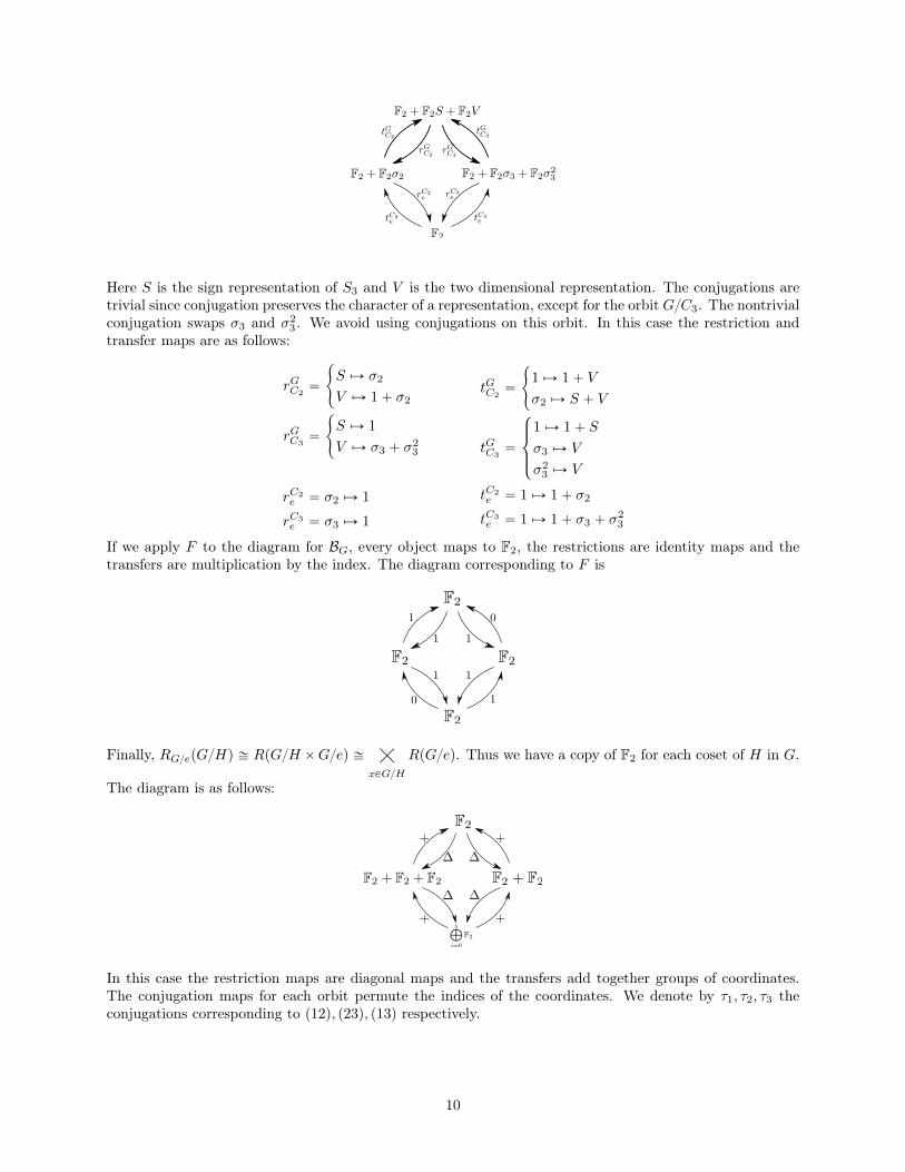
Here S is the sign representation of S3 and V is the two dimensional representation. The conjugations aretrivial since conjugation preserves the character of a representation, except for the orbit G{C3. The nontrivialconjugation swaps σ3 and σ2

3 . We avoid using conjugations on this orbit. In this case the restriction andtransfer maps are as follows:

rGC2“

#

S ÞÑ σ2

V ÞÑ 1` σ2

rGC3“

#

S ÞÑ 1

V ÞÑ σ3 ` σ23

rC2e “ σ2 ÞÑ 1

rC3e “ σ3 ÞÑ 1

tGC2“

#

1 ÞÑ 1` V

σ2 ÞÑ S ` V

tGC3“

$

’

&

’

%

1 ÞÑ 1` S

σ3 ÞÑ V

σ23 ÞÑ V

tC2e “ 1 ÞÑ 1` σ2

tC3e “ 1 ÞÑ 1` σ3 ` σ

23

If we apply F to the diagram for BG, every object maps to F2, the restrictions are identity maps and thetransfers are multiplication by the index. The diagram corresponding to F is

Finally, RG{epG{Hq – RpG{H ˆG{eq –ą

xPG{H

RpG{eq. Thus we have a copy of F2 for each coset of H in G.

The diagram is as follows:

In this case the restriction maps are diagonal maps and the transfers add together groups of coordinates.The conjugation maps for each orbit permute the indices of the coordinates. We denote by τ1, τ2, τ3 theconjugations corresponding to p12q, p23q, p13q respectively.

10

Now we must verify that the sequence given above is exact. As with the case G “ Cm, the map from R toF is the augmentation map given in Example 3.15. The kernel of this map applied to each orbit takes theform:

The transfer and restriction maps for this kernel are induced by the transfer and restriction maps for R. Wemust show that multiplication by V maps surjectively onto this kernel. Using characters we can calculate thefollowing products of representations: s2 “ 1, V 2 “ 1`S`V , SV “ V . If we multiply F2`F2S`F2V by Vwe get F2V `F2V `F2p1`S`V q – F2pS´1q`F2V . Multiplying any element of G{H by V means multiplyingthat element by the rGHpV q. Thus V ¨pF2`F2σ3`F2σ

23q “ pσ3`σ

23qpF2`F2σ3`F2σ

23q. Any choice of coefficients

for this expression gives an element of the kernel. For G{C2, V ¨pF2`F2σ2q “ p1`σ2qpF2`F2σ2q “ F2p1`σ2q.For G{e, rGe pV q “ 0, so RpG{eq maps onto 0. Thus, the map that multiplies by V surjects onto the kernelof the previous map.

The kernel of multiplication by V is

We must map from RG{e onto this kernel. This map is 1b r, which, as before, adds together the entries ineach vector in RpG{Hq. The kernel of this map is, for any orbit G{H, the set of vectors VH so that the sumof the entries in each vector is zero.

We must now map from RG{e onto the kernel shown above. This is accomplished by the map 1b pτ1 ` τ2 `τ3 ´ 1q. If we apply this map to pa, b, cq P RG{epG{C2q, pτ1 ` τ2 ` τ3qpa, b, cq ´ pa, b, cq “ pa ` b ` c, a `b ` c, a ` b ` cq ´ pa, b, cq “ pb ` c, a ` c, a ` bq. This is a map onto the kernel of the previous map in thecase of G{C2. In the case of G{C2, pτ1 ` τ2 ` τ3qpa, bq ´ pa, bq “ pa ` b, a ` bq, as desired. For RG{epG{eq,1bpτ1` τ2` τ3´ 1q is a map of rank five. Thus it is a surjection onto the kernel of the previous map whichhas dimension five. For RG{epG{Gq, this map is the zero map. For each of the above orbits, the kernel ofthe map 1b pτ1 ` τ2 ` τ3 ´ 1q is one dimensional. Thus the next kernel looks like

11

The map 1 b t maps from R into RG{e via the restriction rHe and surjects onto the kernel of the previousmap. This gives us a four periodic projective resolution.

5.2 Computation of ExtRpF, F q

Applying HomRp´, F q we have

HomRpR,F qVÝÑ HomRpR,F q

Hompr,1qÝÝÝÝÝÑ HomRpRG{e, F q

Hompτ,1q´1ÝÝÝÝÝÝÝÑ HomRpRG{e, F q

Hompt,1qÝÝÝÝÝÑ F Ñ ¨ ¨ ¨

Using the identities for HomRp´, F q and the fact that the action of V on F is multiplication by 2 which is0, this simplifies to

F0ÝÑ F

Hompr,1qÝÝÝÝÝÑ Hompr´, G{es, F q

Hompτ1`τ2`τ3,1q´1ÝÝÝÝÝÝÝÝÝÝÝÝÑ Hompr´, G{es, F q

Hompt,1qÝÝÝÝÝÑ F ÝÑ ¨ ¨ ¨

We shall apply this sequence to each orbit in BG and compute ExtRpF, F q.

For G{G we have

F20ÝÑ F2

Id.ÝÝÑ F2

0ÝÑ F2

0ÝÑ F2 ÝÑ ¨ ¨ ¨

For G{C2 we have

F20ÝÑ F2

∆ÝÑ F2 ` F2 ` F2

τ1`τ2`τ3´1ÝÝÝÝÝÝÝÝÑ F2 ` F2 ` F2

0ÝÑ F2 ÝÑ ¨ ¨ ¨

where ∆ denotes the diagonal map. For G{C3 we have

F20ÝÑ F2

∆ÝÑ F2 ` F2

τ1`τ2`τ3´1ÝÝÝÝÝÝÝÝÑ F2 ` F2

`ÝÑ F2 ÝÑ ¨ ¨ ¨

where ∆ denotes the diagonal map, and ` denotes the augmentation map that adds coordinates. For G{ewe have

F20ÝÑ F2

∆ÝÑ

5à

i“0

F2τ1`τ2`τ3´1ÝÝÝÝÝÝÝÝÑ

5à

i“0

F2`ÝÑ F2 ÝÑ ¨ ¨ ¨

where ∆ denotes the diagonal map, and ` denotes the augmentation map that adds coordinates.

We summarize the results of the ExtRpF, F q computations for G “ S3 in the following theorem:

Theorem 5.3. For the orbit G{G, Ext0RpF, F qpG{Gq “ F2, and for j ą 0,

Ext jRpF, F qpG{Gq “

$

’

’

’

&

’

’

’

%

0 j “ 1

0 j “ 2

F2 j “ 3

F2 j “ 0

pmod 4q

For the orbit G{C2, Ext0RpF, F qpG{Gq “ F2, and for j ą 0,

12

Ext jRpF, F qpG{C2q “

$

’

’

’

&

’

’

’

%

0 j “ 1

0 j “ 2

F2 j “ 3

F2 j “ 0

pmod 4q

For the orbit G{C3,


#

F2 j “ 0

0 j ą 0

For the orbit G{e,


#

F2 j “ 0

0 j ą 0

For both Ext3RpF, F q and Ext4

RpF, F q,Green functors, we have that rHK “ 1, tHK “ 1, and the conjugations arethe identity.

5.3 Ring Structure of Ext

We now wish to identify the ring structure of Ext iRpF, F qpG{C2q and Ext iRpF, F qpG{Gq. For the first case,Ext iRpF, F qpG{C2q corresponds to chain maps PC2

‚ì Ñ PC2‚ . However, we already computed the chain maps

and the products for G “ C2 in the previous section, and this gives us the ring structure:

Theorem 5.4. Over the field F2, ExtRpF, F qpS3{C2q is given by

ExtRpF, F qpG{C2q “ F2ry3, x4s{py23 “ 0q.


For G{G, elements of Ext3RpF, F qpG{Gq correspond to the chain maps P‚`3 Ñ P‚. This follows since H “ G,

so ResGH “ ResGG is trivial. Similarly elements of Ext4RpF, F qpG{Gq correspond to the chain maps P‚`4 Ñ P‚.

We compute these chain maps in the following proposition.

Proposition 5.5. The chain map f : PCm‚`3`4k Ñ PCm‚ given by the vertical maps in the following commu-

tative diagram represent nonzero classes in Ext3`4kR pF, F qpCn{Cmq.

The chain map g : PCm‚`4k Ñ PCm‚ given by the vertical maps in the following commutative diagram represent

nonzero classes in Ext4kR pF, F qpCn{Cmq.

13

As before, these chain maps represent the classes x3 and x4. Now we must compute the compositionsP3`4

gÝÑ P3

fÝÑ P0

augÝÝÑ F , P4`3

fÝÑ P4

gÝÑ P0

augÝÝÑ F , and P4`4

gÝÑ P4

gÝÑ P0

augÝÝÑ F . Explicitly these maps

are RG{er1,0,¨¨¨ ,0sÝÝÝÝÝÝÑ RG{e

1ÝÑ R

augÝÝÑ F , RG{e

1ÝÑ R

1ÝÑ R

augÝÝÑ F , and R 1

ÝÑ R1ÝÑ R

augÝÝÑ F . These maps all

compose to 1. We have arrived at the following theorem:

Theorem 5.6. Over the field F2, ExtRpF, F qpS3{S3q is given by

ExtRpF, F qpG{Gq “ F2ry3, x4s{py23 “ 0q.


14

References[1] Joana Ventura. Homological algebra for the representation green functor for abelian groups. Transactions

of the American Mathematical Society, 357:2253–2289, 2004.

[2] Serge Bouc. Green Functors and G-sets. Lecture Notes in Mathematics. Springer, 1997.

[3] Andreas Dress. Contributions to the theory of induced representations. Lecture Notes in Mathematics.Springer, 1973.

[4] Peter Webb. A guide to mackey functors. www.math.umn.edu/ webb/Publications/GuideToMF.ps.

Documents

Homological Algebra over the Representation Green Functor