Homogenization, Symmetry, and Periodization in …aalexan3/articles/homog-paper.pdf · Homogenization, Symmetry, and Periodization in Diffusive Random ... Lions & Papanicolaou

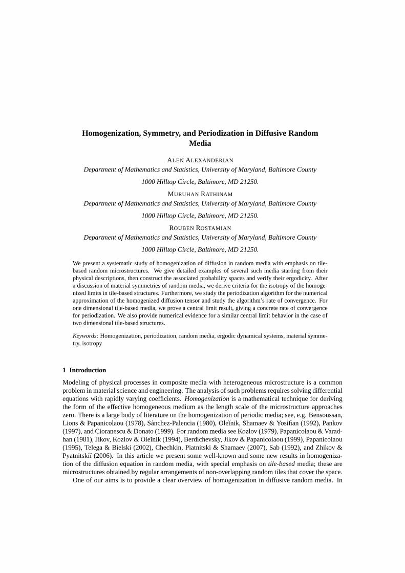
Homogenization, Symmetry, and Periodization in DiffusiveRandomMedia

ALEN ALEXANDERIAN

Department of Mathematics and Statistics, University of Maryland, Baltimore County

1000 Hilltop Circle, Baltimore, MD 21250.

MURUHAN RATHINAM



ROUBEN ROSTAMIAN



We present a systematic study of homogenization of diffusion in random media with emphasis on tile-based random microstructures. We give detailed examples of severalsuch media starting from theirphysical descriptions, then construct the associated probability spacesand verify their ergodicity. Aftera discussion of material symmetries of random media, we derive criteriafor the isotropy of the homoge-nized limits in tile-based structures. Furthermore, we study the periodizationalgorithm for the numericalapproximation of the homogenized diffusion tensor and study the algorithm’s rate of convergence. Forone dimensional tile-based media, we prove a central limit result, giving aconcrete rate of convergencefor periodization. We also provide numerical evidence for a similar central limit behavior in the case oftwo dimensional tile-based structures.

Keywords: Homogenization, periodization, random media, ergodic dynamical systems, material symme-try, isotropy

1 Introduction

Modeling of physical processes in composite media with heterogeneous microstructure is a commonproblem in material science and engineering. The analysis of such problems requires solving differentialequations with rapidly varying coefficients.Homogenizationis a mathematical technique for derivingthe form of the effective homogeneous medium as the length scale of the microstructure approacheszero. There is a large body of literature on the homogenization of periodic media; see, e.g. Bensoussan,Lions & Papanicolaou (1978), Sanchez-Palencia (1980), Oleınik, Shamaev & Yosifian (1992), Pankov(1997), and Cioranescu & Donato (1999). For random media seeKozlov (1979), Papanicolaou & Varad-han (1981), Jikov, Kozlov & Oleınik (1994), Berdichevsky, Jikov & Papanicolaou (1999), Papanicolaou(1995), Telega & Bielski (2002), Chechkin, Piatnitski & Shamaev (2007), Sab (1992), and Zhikov &Pyatnitskiı (2006). In this article we present some well-known and somenew results in homogeniza-tion of the diffusion equation in random media, with specialemphasis ontile-basedmedia; these aremicrostructures obtained by regular arrangements of non-overlapping random tiles that cover the space.

One of our aims is to provide a clear overview of homogenization in diffusive random media. In

2 Alexanderian, Rathinam, Rostamian

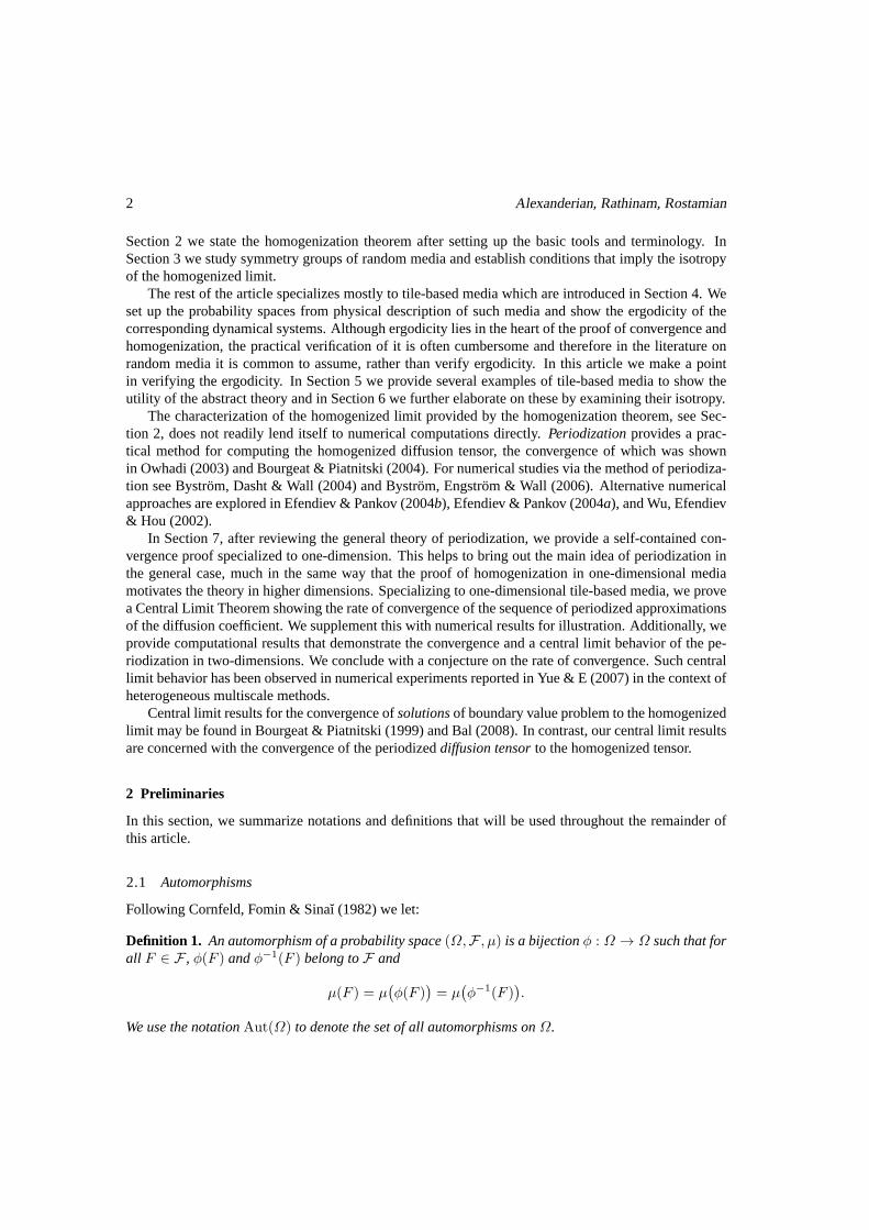
Section 2 we state the homogenization theorem after settingup the basic tools and terminology. InSection 3 we study symmetry groups of random media and establish conditions that imply the isotropyof the homogenized limit.

The rest of the article specializes mostly to tile-based media which are introduced in Section 4. Weset up the probability spaces from physical description of such media and show the ergodicity of thecorresponding dynamical systems. Although ergodicity lies in the heart of the proof of convergence andhomogenization, the practical verification of it is often cumbersome and therefore in the literature onrandom media it is common to assume, rather than verify ergodicity. In this article we make a pointin verifying the ergodicity. In Section 5 we provide severalexamples of tile-based media to show theutility of the abstract theory and in Section 6 we further elaborate on these by examining their isotropy.

The characterization of the homogenized limit provided by the homogenization theorem, see Sec-tion 2, does not readily lend itself to numerical computations directly. Periodizationprovides a prac-tical method for computing the homogenized diffusion tensor, the convergence of which was shownin Owhadi (2003) and Bourgeat & Piatnitski (2004). For numerical studies via the method of periodiza-tion see Bystrom, Dasht & Wall (2004) and Bystrom, Engstrom & Wall (2006). Alternative numericalapproaches are explored in Efendiev & Pankov (2004b), Efendiev & Pankov (2004a), and Wu, Efendiev& Hou (2002).

In Section 7, after reviewing the general theory of periodization, we provide a self-contained con-vergence proof specialized to one-dimension. This helps tobring out the main idea of periodization inthe general case, much in the same way that the proof of homogenization in one-dimensional mediamotivates the theory in higher dimensions. Specializing toone-dimensional tile-based media, we provea Central Limit Theorem showing the rate of convergence of the sequence of periodized approximationsof the diffusion coefficient. We supplement this with numerical results for illustration. Additionally, weprovide computational results that demonstrate the convergence and a central limit behavior of the pe-riodization in two-dimensions. We conclude with a conjecture on the rate of convergence. Such centrallimit behavior has been observed in numerical experiments reported in Yue & E (2007) in the context ofheterogeneous multiscale methods.

Central limit results for the convergence ofsolutionsof boundary value problem to the homogenizedlimit may be found in Bourgeat & Piatnitski (1999) and Bal (2008). In contrast, our central limit resultsare concerned with the convergence of the periodizeddiffusion tensorto the homogenized tensor.

2 Preliminaries

In this section, we summarize notations and definitions thatwill be used throughout the remainder ofthis article.

2.1 Automorphisms

Following Cornfeld, Fomin & Sinaı (1982) we let:

Definition 1. An automorphism of a probability space(Ω,F , µ) is a bijectionφ : Ω → Ω such that forall F ∈ F , φ(F ) andφ−1(F ) belong toF and

µ(F ) = µ(

φ(F ))

= µ(

φ−1(F ))

.

We use the notationAut(Ω) to denote the set of all automorphisms onΩ.

Homogenization, Symmetry, and Periodization of Random Media 3

2.2 Notation for matrices

We writeRn×n for the space ofn× n matrices. We let:

Rn×nsym = the subspace of symmetric matrices inR

n×n

Rn×north = the orthogonal group of matrices inRn×n

Rn×north+ = the proper orthogonal group of matrices inRn×n.

For any0 < ν1 6 ν2 we let

E(ν1, ν2) = A ∈ Rn×nsym : ν1|ξ|2 6 ξ ·Aξ 6 ν2|ξ|2 ∀ξ ∈ R

n

Let (S,Σ) be a measurable space. IfA : S → Rn×nsym is a measurable mapping such thatA(x) ∈

E(ν1, ν2) for all x ∈ S (or almost allx ∈ S if there is a measure on(S,Σ)) then we sayA belongs toE(ν1, ν2, S).

2.3 The dynamical system

An n-dimensional measure-preserving dynamical systemT on Ω is a family of automorphismsTx :Ω → Ω, parametrized byx ∈ R

n, satisfying:

1. Tx+y = Tx Ty for all x, y ∈ Rn,

2. T0 = I, whereI is the identity map onΩ.

3. The dynamical system isjointly measurable onRn × Ω in the sense that the mapping(x, ω) 7→Tx(ω) is B(Rn)⊗F/F measurable, whereB(Rn) is the Borelσ-algebra onRn.

A setE ⊂ Ω is said to beinvariant under the dynamical systemT if T−1x (E) ⊂ E for all x ∈ R

n.

Definition 2. The dynamical systemT is ergodicif all its invariant sets have measure of either zero orone.

The dynamical systemT is ergodic if and only if for every measurable functionf : Ω → R thefollowing holds (Cornfeld et al. 1982):

[

f(

Tx(ω))

= f(ω) for all x and almost allω]

⇒ f = constant a.s. (1)

Corresponding to a functionf : Ω → X (whereX is any set) we define the functionfT : Rn×Ω →X by

fT(

x, ω)

= f(

Tx(ω))

, x ∈ Rn, ω ∈ Ω.

For eachω ∈ Ω, the functionfT(

·, ω)

: Rn → X is called therealizationof f for thatω.

2.4 Solenoidal and potential vector fields

Let (Ω,F , µ) be a probability space with theσ-algebraF and a measureµ. We will write EX fortheexpected valueof the random variableX onΩ. That is,EX =

∫

ΩX dµ.


Let T be ann-dimensional measure-preserving dynamical system onΩ and letL2(Ω;Rn) be thespace of square integrable vector fieldsf : Ω → R

n. We define:

L2pot(Ω) = f ∈ L2(Ω;Rn) : fT (·, ω) is a potential field onRn for almost allω ∈ ΩL2sol(Ω) = f ∈ L2(Ω;Rn) : fT (·, ω) is a solenoidal field onRn for almost allω ∈ Ω

V2pot(Ω) =

f ∈ L2pot(Ω) : E f = 0

.

V2sol(Ω) =

f ∈ L2sol(Ω) : E f = 0

.

These spaces induce orthogonal decompositions ofL2(Ω;Rn), cf. Jikov et al. (1994, page 228):

Theorem 1(Weyl’s Decomposition). If the dynamical systemT is ergodic, then:

L2(Ω;Rn) = V2pot(Ω)⊕ L2

sol(Ω) = V2sol(Ω)⊕ L2

pot(Ω). (2)

2.5 Homogenization

Consider a matrix-valued functionA : Rn → R

n×nsym . Assume thatA ∈ E(ν1, ν2,R

n) for some0 < ν1 6 ν2.

For anyǫ > 0 let Aǫ(x) = A(x/ǫ). Then we say thatA admits homogenizationif there exists aconstant symmetric positive definite matrixA0 such that for any bounded domainD ⊂ R

n and anyf ∈ H−1(D) the solutionsuǫ andu0 of the boundary value problems

− div(Aǫ∇uǫ) = f onDuǫ = 0 on∂D and

− div(A0∇u0) = f onDu0 = 0 on∂D

(3)

satisfy, asǫ → 0:

uǫ u0 in H10 (D),

Aǫ∇uǫ A0∇u0 in L2(D).

It is a classic result that ifA is periodic onRn then it admits homogenization. The basic references inBensoussan et al. (1978), Sanchez-Palencia (1980), Cioranescu & Donato (1999), Oleınik et al. (1992),and Pankov (1997) represent but a small sample of the vast literature on the subject.

The main focus of our article is on the random case, that is, the boundary value problem:

− div(

A(x

ǫ, ω

)

∇u(x, ω))

= f(x) in D,

u(x, ω) = 0 on∂D,(4)

whereω ∈ Ω and(Ω,F , µ) is a probability space.A fully developed theory exists for the case whenA : Rn ×Ω → R

n×nsym is a stationary and ergodic

random field. The early work in the area by Kozlov (1979) and Papanicolaou & Varadhan (1981) isgreatly expanded upon in the monograph Jikov et al. (1994). In this theory, without loss of generality,one begins with a functionA ∈ E(ν1, ν2, Ω) and considers its realizationsA(x, ω) = AT (x, ω) withrespect to ann-dimensional ergodic dynamical systemT . Concerning this, we have:


Theorem 2. (Jikov et al. 1994, Theorem 7.4) LetA ∈ E(ν1, ν2, Ω) and T be ann-dimensionalmeasure-preserving ergodic dynamical system onΩ. Then, for almost allω ∈ Ω, the realizationAT (·, ω) admits a homogenizationA0. Moreover,A0 is positive-definite, independent ofω, and ischaracterized by,

ξ · A0ξ = infv∈V2

pot(Ω)

∫

Ω

(ξ + v) · A(ξ + v) dµ, ∀ξ ∈ Rn. (5)

Remark 1. Although Theorem 2 gives a complete characterization of thelimiting homogenized prob-lem, the characterization is not constructive because it involves integrating on an abstract probabilityspace. Themethod of periodization(Owhadi 2003, Bourgeat & Piatnitski 2004), described in Section 7,provides a concrete way of approximatingA0 numerically.

2.6 Linear algebra

Here we collect some observations and results from linear algebra, which will be needed in our discus-sions of symmetry and isotropy.

A subspaceV ⊆ Rn is said to be invariant underA ∈ R

n×n if AV ⊆ V .

Definition 3 (Irreducible group (Weyl 1946)). Let G be a matrix group inRn×n. We callG an irre-ducible groupif it has the following property: If a subspaceV ofRn is invariant underQ for all Q ∈ G,thenV is either0 or Rn.

As an example of an irreducible group inR2×2 consider the cyclic rotation group of order 4:G1 =I,R90, R180, R270, whereRθ ∈ R

2×2 denotes rotation by angleθ about the origin. Another exampleof an irreducible group isRn×n

orth+ . An example of a group which is not irreducible isG2 = I,R180because it leaves any one-dimensional subspace invariant.

The following result is a simple case of Schur’s Lemma (Schur1905, Fulton & Harris 1991, James& Liebeck 2001) which is a basic result in group representation theory.

Lemma 1. LetG be an irreducible group inRn×n and supposeA is a symmetric matrix that commuteswith everyQ ∈ G. ThenA is a scalar multiple of identity.

Proof. Let α be an eigenvalue ofA, and define the mappingB = A − αI. It follows that,BQ = QBfor all Q ∈ G. Moreover, sinceα is an eigenvalue ofA, Null(B) = Null(A − αI) 6= 0. Now, ifx ∈ Null(B), thenBQx = QBx = 0, that isQx ∈ Null(B). Therefore,Null(B) is invariant underQ for all Q ∈ G. SinceG is irreducible (andNull(B) 6= 0), it follows thatNull(B) = R

n. That is,B = 0, and henceA = αI.

Let us give an example that shows that the condition of irreducibility in Lemma 1 cannot be removed.Consider the symmetric2× 2 matrixA =

(

a bb c

)

. SupposeA commutes with elements of the reduciblegroupG = I,R whereR =

(

1 00 −1

)

. ThenAR = RA implies thatb = 0 whenceA = ( a 00 c ) where

a andc are arbitrary.The following two results give conditions under which a matrix is a multiple of identity in two and

three dimensions.

Proposition 1. LetS ∈ R2×2sym andQ ∈ R

2×2orth+ \±I. ThenS commutes withQ if and only ifS = λI.

Proof. SupposeSQ = QS. The only subspace ofR2 invariant underQ is either0 orR2. Hence, theresult follows from Lemma 1. The converse implication is trivial.


Proposition 2. Let u and v be linearly independent vectors inR3. Fix α and β in (0, π). SupposeS ∈ R

3×3sym commutes withRα

u andRβv . ThenS is a multiple of identity.

Proof. We will show that the only subspaces ofR3 invariant under bothRα

u andRβv are0 andR3;

the result would then follow from Lemma 1. Note that the only subspaces ofR3 invariant underRαu are:

0, spanu, spanu⊥, R3.

Similarly, the only subspaces ofR3 invariant underRβv are:

0, spanv, spanv⊥, R3.

Sinceu andv are linearly independent, it follows that0 andR3 are the only subspaces ofR3 invariant

under bothRαu andRβ

v .

3 Symmetries of random media and questions of isotropy

In this section we develop an abstract framework and study interesting but nontrivial conditions on theconductivity matrixAT (x, ω) which imply that the homogenized conductivity matrix,A0, is a multipleof identity, that is, the homogenized medium is isotropic.

Definition 4. LetQ be an orthogonal matrix andT be a dynamical system. We say thatA ∈ E(ν1, ν2, Ω)is Q-invariantif there existsζ ∈ Aut(Ω) such that:

AT

(

x, ζ(ω))

= QAT (QTx, ω)QT ,

for almost allx ∈ Rn and almost allω ∈ Ω.

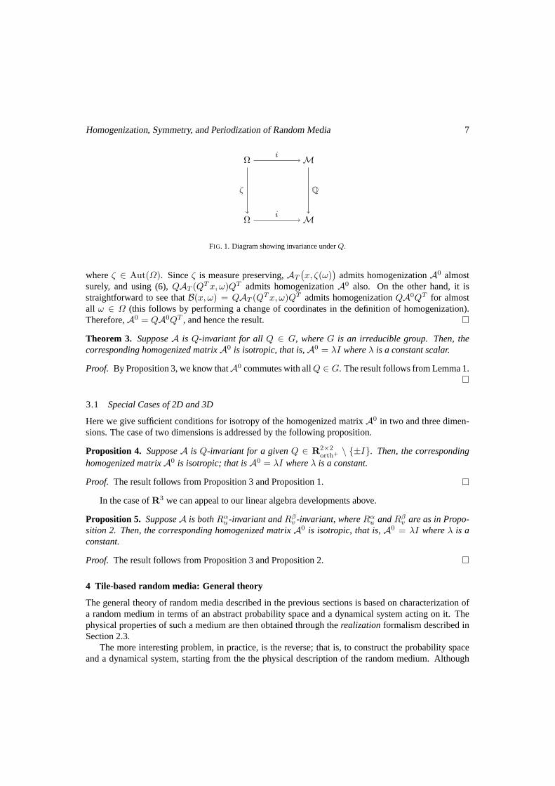
Remark 2. The above definition can be best understood in terms of the commutative diagram in Fig-ure 1. LetM = E(ν1, ν2,R

n), and leti : Ω → M : ω 7→ AT (·, ω); that is,i(ω) is the conductivitytensor field corresponding toω ∈ Ω. GivenQ ∈ R

n×north , we defineQ : M → M by

(QAT )(x, ω) = QAT (QTx, ω)QT .

From Definition 4, it follows that the diagram in Figure 1 commutes. This means that any collectionM ⊂ M of conductivity tensors and their rotated versionsQM are equally likely, that is,µ

(

i−1(M))

=

µ(

i−1(QM))

. This follows since,

µ(

i−1(QM))

= µ(

ζ−1i−1(QM))

= µ(

i−1Q−1Q(M))

= µ(

i−1(M))

,

where the first equality holds sinceζ is measure preserving, and the second equality holds since thediagram in Figure 1 commutes.

Proposition 3. SupposeA is Q-invariant for a givenQ ∈ Rn×north+ . Then the corresponding homoge-

nized matrixA0 commutes withQ, that is,A0Q = QA0.

Proof. We know by Theorem 2 thatAT (x, ω) admits homogenizationA0 almost surely. Moreover, byQ-invariance

AT

(

x, ζ(ω))

= QAT (QTx, ω)QT , (6)


Ω M

Ω M

i

ζ Q

i

FIG. 1. Diagram showing invariance underQ.

whereζ ∈ Aut(Ω). Sinceζ is measure preserving,AT

(

x, ζ(ω))

admits homogenizationA0 almostsurely, and using (6),QAT (Q

Tx, ω)QT admits homogenizationA0 also. On the other hand, it isstraightforward to see thatB(x, ω) = QAT (Q

Tx, ω)QT admits homogenizationQA0QT for almostall ω ∈ Ω (this follows by performing a change of coordinates in the definition of homogenization).Therefore,A0 = QA0QT , and hence the result.

Theorem 3. SupposeA is Q-invariant for all Q ∈ G, whereG is an irreducible group. Then, thecorresponding homogenized matrixA0 is isotropic, that is,A0 = λI whereλ is a constant scalar.

Proof. By Proposition 3, we know thatA0 commutes with allQ ∈ G. The result follows from Lemma 1.

3.1 Special Cases of 2D and 3D

Here we give sufficient conditions for isotropy of the homogenized matrixA0 in two and three dimen-sions. The case of two dimensions is addressed by the following proposition.

Proposition 4. SupposeA is Q-invariant for a givenQ ∈ R2×2orth+ \ ±I. Then, the corresponding

homogenized matrixA0 is isotropic; that isA0 = λI whereλ is a constant.

Proof. The result follows from Proposition 3 and Proposition 1.

In the case ofR3 we can appeal to our linear algebra developments above.

Proposition 5. SupposeA is bothRαu -invariant andRβ

v -invariant, whereRαu andRβ

v are as in Propo-sition 2. Then, the corresponding homogenized matrixA0 is isotropic, that is,A0 = λI whereλ is aconstant.

Proof. The result follows from Proposition 3 and Proposition 2.

4 Tile-based random media: General theory

The general theory of random media described in the previoussections is based on characterization ofa random medium in terms of an abstract probability space anda dynamical system acting on it. Thephysical properties of such a medium are then obtained through therealizationformalism described inSection 2.3.

The more interesting problem, in practice, is the reverse; that is, to construct the probability spaceand a dynamical system, starting from the the physical description of the random medium. Although


this process is an essential aspect of the modeling of randommedia, it is rarely brought out and analyzedin detail in the literature. It is among our goals in this article to bring this issue to focus. As we will seein the following sections, the process is not quite trivial.

In Section 4.1 we introduce the setY of all possible tiles, and put a probability measure on it. Inthesimplest case of a “black-white” checkerboard where the tiles can be only one of two possibilities, the setY consists of two elements and the probability measure indicates the likelihood of occurrence of one orthe other tile. Subsequently, we useY as building blocks for the sample space of all possible realizations.In Section 4.2 we construct a dynamical systemTxx∈Rn on the probability space which tiles the spacewith random tiles from the setY . We show that the dynamical system is measure preserving andergodic.In Section 4.3 we start with the physical description of the conductivity tensorA(y) of each tiley in Yand construct the overall conductivity tensorAT (x, ω) that enters the boundary value problem (3). Theconstructions are rather abstract but they are sufficientlygeneral to include many interesting applicationsas illustrated in Section 5.

4.1 The probability space

Let the setY parametrize the possible choices for a tile and consider theprobability space(Y,FY , µY ),whereFY is an appropriateσ-algebra andµY is a probability measure. Form the product space(S,FS , µS) =

∏

Zn(Y,FY , µY ), where theσ-algebraFS is the productσ-algebra andµS is the productmeasure. Finally, to account for translations, define the overall probability space

(Ω,F , µ) = (S,FS , µS)⊗(

Torn,B(Torn),Leb

)

, (7)

whereTorn = [0, 1)n is then-dimensional unit cube with the opposite faces identified,B(Torn) is theBorelσ-algebra onTorn, andLeb is the Lebesgue measure.

4.2 The dynamical system and ergodicity

We construct the measure-preserving and ergodic dynamicalsystemT that enters the definition of theconductivity matrix in the boundary value problem (4). An elements ∈ S has form

s = sjj∈Zn , sj ∈ Y,

and an elementω ∈ Ω has form,

ω = (s, τ) s ∈ S, τ ∈ Torn. (8)

First we define the dynamical systemTzz∈Zn onS by

Tz

(

sjj∈Zn

)

= sj+zj∈Zn .

Let us define the projection operatorsP1 : Rn → Zn andP2 : Rn → Tor

n by

P1(x) = ⌊x⌋, x ∈ Rn,

P2(x) = x− ⌊x⌋, x ∈ Rn.

Here⌊x⌋ is the vector whose elements are the greatest integers less or equal to the corresponding ele-ments inx. Note that eachx ∈ R

n has the unique decomposition

x = P1(x) + P2(x).


Next, define the dynamical systemRxx∈Rn onTorn by

Rx(τ) = P2(x+ τ), τ ∈ Torn.

Finally, we define the dynamical systemTxx∈Rn onΩ by

Tx(ω) = Tx(s, τ) =(

TP1(x+τ)(s), Rx(τ))

, s ∈ S, τ ∈ Torn. (9)

Let us verify the group property for the dynamical system above. ClearlyT0(ω) = ω for all ω ∈ Ω.Moreover, we showTx Ty = Tx+y for all x andy in R

n as follows. Letω = (s, τ) be an element ofΩ, as described in (8), and note that

Tx+y(ω) = Tx+y(sj, τ) =(

sj+P1(x+y+τ), P2(x+ y + τ))

. (10)

On the other hand

Tx

(

Ty(ω))

= Tx

(

Ty

(

sj, τ)

)

= Tx

(

sj+P1(y+τ), P2(y + τ))

=(

sj+P1(y+τ)+P1(x+P2(y+τ)), P2

(

x+ P2(y + τ))

)

. (11)

Sinceu+ P1(v) = P1(u+ v) for everyu ∈ Zn, v ∈ R

n, we have

P1(y + τ) + P1

(

x+ P2(y + τ))

= P1

(

x+ P1(y + τ) + P2(y + τ))

= P1(x+ y + τ). (12)

Also, sinceP2(u+ v) = P2(v) for everyu ∈ Zn andv ∈ R

n, we have,

P2

(

x+ P2(y + τ))

= P2

(

x+ P1(y + τ) + P2(y + τ))

= P2(x+ y + τ). (13)

Combining (11), (12), and (13) we obtain

Tx

(

Ty(ω))

=(

sj+P1(x+y+τ), P2(x+ y + τ))

= Tx+y(ω),

where the last equality follows from (10).The measure preserving property of the dynamical systemTxx∈Rn follows from the following

proposition:

Proposition 6. The dynamical systemTxx∈Rn defined in(9) is measure preserving.

Proof. Let x ∈ Rn be fixed but arbitrary. It is sufficient so show thatµ

(

T−1x (A × B)

)

= µ(A × B)for all rectanglesA × B ∈ F , whereA ∈ FS andB ∈ B(Torn). Note that we can partitionTorn asfollows,

Torn =

⊎

j∈Zn

Ej , Ej = τ ∈ Torn : P1(x+ τ) = j,

where⊎

denotes a disjoint union. Note also that only finitely many ofEj are non-empty. Then, for arectangleA×B in F we have

T−1x (A×B) =

⊎

j

(

T−1j (A)×

[

R−1x (B) ∩ Ej

]

)

.


SinceTj andRx are measure preserving, we conclude that

µ(

T−1x (A×B)

)

=∑

j

µ(

T−1j (A)×

[

R−1x (B) ∩ Ej

]

)

=∑

j

µS(A) Leb[R−1x (B) ∩ Ej ]

= µS(A)∑

j

Leb[

R−1x (B) ∩ Ej

]

= µS(A) Leb(

R−1x (B)

)

= µS(A) Leb(B) = µ(A×B). (14)

What remains to show is ergodicity of the dynamical systemTx. It is well-known that the dynamicalsystemTzz∈Zn is ergodic (Walters 1982, Cornfeld et al. 1982). We use this to prove the following:

Proposition 7. The dynamical systemTxx∈Rn defined in(9) is ergodic.

Proof. Let f be a measurable function onΩ which is invariant underT , that is,

f(

Tx(ω))

= f(ω) ∀x ∈ Rn, µ-a.s.. (15)

Recall thatω ∈ Ω has the formω = (s, τ), with s ∈ S andτ ∈ Torn. Now by (15) we have also

f(

Tz(ω))

= f(ω), for all z ∈ Zn. SinceRz(τ) = τ for z ∈ Z

n,

f(s, τ) = f(

Tz(s, τ))

= f(

Tz(s), Rz(τ))

= f(

Tz(s), τ)

.

Lettingfτ (s) = f(s, τ), this takes the form

fτ(

Tz(s))

= fτ (s) ∀z ∈ Zn. (16)

We knowfτ (s) is measurable onS. SinceTzz∈Zn is ergodic, then (16) implies that for eachτ , fτ isconstantµS-a.s. . Therefore,

f(s, τ) = φ(τ) s ∈ S, τ ∈ Torn. (17)

Next, using (15) again we have

f(

Tt(ω))

= f(ω) ∀t ∈ Torn. (18)

Now, using (17) we have

f(

Tt(ω))

= f(

TP1(t+τ)(s), Rt(τ))

= φ(Rtτ);

also,f(ω) = f(s, τ) = φ(τ). Therefore, (18) gives that

φ(

Rt(τ))

= φ(τ) ∀t ∈ Torn, a.e. (19)

Finally, recalling ergodicity of the dynamical systemRtt∈Torn , we get thatφ(τ) ≡ const a.e. andhence,f ≡ const a.e. Thus, the assertion of the proposition follows from (1).


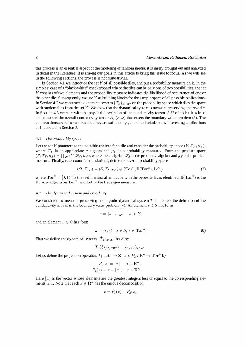
FIG. 2. Typical realizations of random “checkerboards” in one,two, or three dimensions.

4.3 The functionAEach elementy in the sample spaceY specifies a certain type of tile. LetA(y) : Torn → R

n×nsym be

the conductivity function associated with that tile. Picks ∈ S and let’s writes = sjj∈Zn . Thisdefines an infinite sequence of tiles with conductivitiesA(sj)j∈Zn . We define the random variableA : Ω → R

n×nsym by

A(ω) = A(s0)(τ), for ω =(

sj, τ)

∈ Ω. (20)

From the definitionTx in (9) we see that:

Tx(ω) = Tx

(

sj, τ)

=(

sj+P1(x+τ), P2(x+ τ))

.

Consequently,A(

Tx(ω))

= A(sσ)(

P2(x+ τ))

, whereσ = P1(x+ τ).

Let us recall thatAT (x, ω) = A(

Tx(ω))

defines the conductivity matrix of the medium and appears asa coefficient in the boundary value problem (4).

5 Tile-based random media: Examples

In the following sections we give several examples to illustrate the construction of concrete probabilityspaces in terms of the medium’s physical properties. In eachcase, it suffices to identify the probabilityspace(Y,FY , µY ) and the tile conductivitiesA(y) as defined in Section 4.3. The machinery developedin Section 4 then assigns the appropriate dynamical system and the conductivity tensorA.

5.1 Checkerboard-like tilings

For our first example we examine a most basic random structure—ann-dimensional medium consistingof then-dimensional cube(0, 1)n and its translations along the integer latticeZ

n in Rn. The cubes/tiles

are identified as eithergray or white with probabilitiesp and1 − p, respectively, wherep ∈ (0, 1).Figure 2 depicts representative samples in 1, 2, and 3 dimensions.


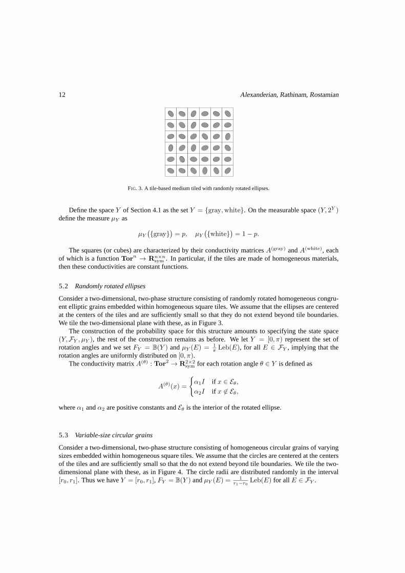
FIG. 3. A tile-based medium tiled with randomly rotated ellipses.

Define the spaceY of Section 4.1 as the setY = gray,white. On the measurable space(Y, 2Y )define the measureµY as

µY

(

gray)

= p, µY

(

white)

= 1− p.

The squares (or cubes) are characterized by their conductivity matricesA(gray) andA(white), eachof which is a functionTorn → R

n×nsym . In particular, if the tiles are made of homogeneous materials,

then these conductivities are constant functions.

5.2 Randomly rotated ellipses

Consider a two-dimensional, two-phase structure consisting of randomly rotated homogeneous congru-ent elliptic grains embedded within homogeneous square tiles. We assume that the ellipses are centeredat the centers of the tiles and are sufficiently small so that they do not extend beyond tile boundaries.We tile the two-dimensional plane with these, as in Figure 3.

The construction of the probability space for this structure amounts to specifying the state space(Y,FY , µY ), the rest of the construction remains as before. We letY = [0, π) represent the set ofrotation angles and we setFY = B(Y ) andµY (E) = 1

π Leb(E), for all E ∈ FY , implying that therotation angles are uniformly distributed on[0, π).

The conductivity matrixA(θ) : Tor2 → R2×2sym for each rotation angleθ ∈ Y is defined as

A(θ)(x) =

α1I if x ∈ Eθ,α2I if x 6∈ Eθ,

whereα1 andα2 are positive constants andEθ is the interior of the rotated ellipse.

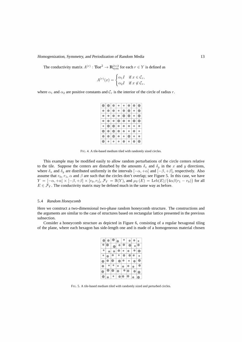
5.3 Variable-size circular grains

Consider a two-dimensional, two-phase structure consisting of homogeneous circular grains of varyingsizes embedded within homogeneous square tiles. We assume that the circles are centered at the centersof the tiles and are sufficiently small so that the do not extend beyond tile boundaries. We tile the two-dimensional plane with these, as in Figure 4. The circle radii are distributed randomly in the interval[r0, r1]. Thus we haveY = [r0, r1], FY = B(Y ) andµY (E) = 1

r1−r0Leb(E) for all E ∈ FY .


The conductivity matrixA(r) : Tor2 → R2×2sym for eachr ∈ Y is defined as

A(r)(x) =

α1I if x ∈ Cr,α2I if x 6∈ Cr,

whereα1 andα2 are positive constants andCr is the interior of the circle of radiusr.

FIG. 4. A tile-based medium tiled with randomly sized circles.

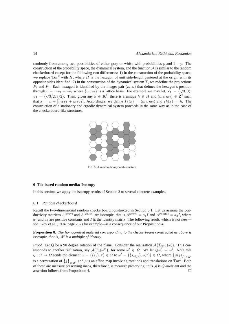
This example may be modified easily to allow random perturbations of the circle centers relativeto the tile. Suppose the centers are disturbed by the amountsδx and δy in the x and y directions,whereδx andδy are distributed uniformly in the intervals[−α,+α] and[−β,+β], respectively. Alsoassume thatr0, r1, α andβ are such that the circles don’t overlap; see Figure 5. In thiscase, we haveY = [−α,+α] × [−β,+β] × [r0, r1], FY = B(Y ), andµY (E) = Leb(E)/

(

4αβ(r1 − r0))

for allE ∈ FY . The conductivity matrix may be defined much in the same way asbefore.

5.4 Random Honeycomb

Here we construct a two-dimensional two-phase random honeycomb structure. The constructions andthe arguments are similar to the case of structures based on rectangular lattice presented in the previoussubsection.

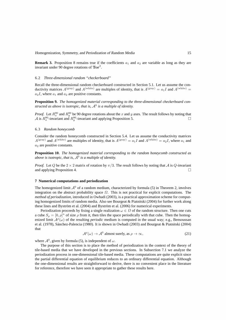
Consider a honeycomb structure as depicted in Figure 6, consisting of a regular hexagonal tilingof the plane, where each hexagon has side-length one and is made of a homogeneous material chosen

FIG. 5. A tile-based medium tiled with randomly sized and perturbed circles.


randomly from among two possibilities of eithergray or white with probabilitiesp and1 − p. Theconstruction of the probability space, the dynamical system, and the functionA is similar to the randomcheckerboard except for the following two differences: 1) In the construction of the probability space,we replaceTor2 with H, whereH is the hexagon of unit side-length centered at the origin with itsopposite sides identified. 2) In the construction of the dynamical systemT , we redefine the projectionsP1 andP2. Each hexagon is identified by the integer pair(m,n) that defines the hexagon’s positionthroughc = mv1 + nv2 wherev1, v2 is a lattice basis. For example we may let,v1 =

⟨√3, 0

⟩

,v2 =

⟨√3/2, 3/2

⟩

. Then, given anyx ∈ R2, there is a uniqueh ∈ H and (m1,m2) ∈ Z

2 suchthat x = h +

[

m1v1 + m2v2

]

. Accordingly, we defineP1(x) = 〈m1,m2〉 andP2(x) = h. Theconstruction of a stationary and ergodic dynamical system proceeds in the same way as in the case ofthe checkerboard-like structures.

FIG. 6. A random honeycomb structure.

6 Tile-based random media: Isotropy

In this section, we apply the isotropy results of Section 3 toseveral concrete examples.

6.1 Random checkerboard

Recall the two-dimensional random checkerboard constructed in Section 5.1. Let us assume the con-ductivity matricesA(gray) andA(white) are isotropic, that isA(gray) = a1I andA(white) = a2I, wherea1 anda2 are positive constants andI is the identity matrix. The following result, which is not new—see Jikov et al. (1994, page 237) for example—is a consequenceof our Proposition 4.

Proposition 8. The homogenized material corresponding to the checkerboard constructed as above isisotropic, that is,A0 is a multiple of identity.

Proof. Let Q be a 90 degree rotation of the plane. Consider the realization A(

TQT x(ω))

. This cor-responds to another realization, sayA

(

Tx(ω′))

, for someω′ ∈ Ω. We let ζ(ω) = ω′. Note thatζ : Ω → Ω sends the elementω =

(

sj, τ)

∈ Ω to ω′ =(

sσ(j), ρ(τ))

∈ Ω, where

σ(j)

j∈Z2

is a permutation of

j

j∈Z2 andρ is an affine map involving rotations and translations onTor2. Both

of these are measure preserving maps, thereforeζ is measure preserving; thusA is Q-invariant and theassertion follows from Proposition 4.


Remark 3. Proposition 8 remains true if the coefficientsa1 anda2 are variable as long as they areinvariant under 90 degree rotations ofTor

2.

6.2 Three-dimensional random “checkerboard”

Recall the three-dimensional random checkerboard constructed in Section 5.1. Let us assume the con-ductivity matricesA(gray) andA(white) are multiples of identity, that isA(gray) = a1I andA(white) =a2I, wherea1 anda2 are positive constants.

Proposition 9. The homogenized material corresponding to the three-dimensional checkerboard con-structed as above is isotropic, that is,A0 is a multiple of identity.

Proof. LetR90x andR90

y be 90 degree rotations about thex andy axes. The result follows by noting thatA is R90

x -invariant andR90y -invariant and applying Proposition 5.

6.3 Random honeycomb

Consider the random honeycomb constructed in Section 5.4. Let us assume the conductivity matricesA(gray) andA(white) are multiples of identity, that isA(gray) = a1I andA(white) = a2I, wherea1 anda2 are positive constants.

Proposition 10. The homogenized material corresponding to the random honeycomb constructed asabove is isotropic, that is,A0 is a multiple of identity.

Proof. LetQ be the2× 2 matrix of rotation byπ/3. The result follows by noting thatA isQ-invariantand applying Proposition 4.

7 Numerical computations and periodization

The homogenized limitA0 of a random medium, characterized by formula (5) in Theorem 2, involvesintegration on the abstract probability spaceΩ. This is not practical for explicit computations. Themethod of periodization, introduced in Owhadi (2003), is a practical approximationscheme for comput-ing homogenized limits of random media. Also see Bourgeat & Piatnitski (2004) for further work alongthese lines and Bystrom et al. (2004) and Bystrom et al. (2006) for numerical experiments.

Periodization proceeds by fixing a single realizationω ∈ Ω of the random structure. Then one cutsa cubeSρ = [0, ρ]n of sizeρ from it, then tiles the space periodically with that cube. Then the homog-enized limitAρ(ω) of the resultingperiodic medium is computed in the usual way; e.g., Bensoussanet al. (1978), Sanchez-Palencia (1980). It is shown in Owhadi (2003) and Bourgeat & Piatnitski (2004)that

Aρ(ω) → A0 almost surely, asρ → ∞, (21)

whereA0, given by formula (5), is independent ofω.The purpose of this section is to place the method of periodization in the context of the theory of

tile-based media that we have developed in the previous sections. In Subsection 7.1 we analyze theperiodization process in one-dimensional tile-based media. These computations are quite explicit sincethe partial differential equation of equilibrium reduces to an ordinary differential equation. Althoughthe one-dimensional results are straightforward to derive, there is no convenient place in the literaturefor reference, therefore we have seen it appropriate to gather these results here.


Theorem 4 gives a self-contained proof of the periodizationtheorem in 1D, via Birkhoff’s ErgodicTheorem. Theorem 5 establishes a central limit result whichprovides the rate of convergence of the dif-fusion coefficient with successive improvements of the periodization approximation. In Subsection 7.2.2we give results of a series of numerical experiments whose purpose is to illustrate the theory developedup to that point.

Section 7.3 reports the results of numerical experiments for periodization in two dimensions. Wepresent numerical evidence for central limit behavior similar to the one-dimensional case and summarizeour results in the form of a conjecture. Such central limit behavior has been observed in numericalexperiments reported in Yue & E (2007) in the context of heterogeneous multiscale methods.

Central limit results for the convergence ofsolutionuǫ to the homogenized limitu0 may be foundin Bourgeat & Piatnitski (1999) and Bal (2008). In contrast,our central limit results are concerned withthe convergence of thediffusion tensorAρ to the homogenized tensorA0.

7.1 Periodization in one-dimensional media

Forω ∈ Ω consider the one-dimensional version of the boundary valueproblem (4):

−(

aT (x, ω)u′(x, ω)

)′= f(x) in D = (0, 1),

u(0, ω) = u(1, ω) = 0,(22)

whereaT (x, ω) = a(

Tx(ω))

anda is the one-dimensional counterpart ofA in Section 2.5. SpecializingTheorem 2 to one dimension, it can be shown that for almost allω ∈ Ω the problem (22) admitshomogenization with the homogenized coefficient given by

a =1

E

1a

. (23)

To approximatea numerically we can use the method of periodization as follows. DenoteSρ =(0, ρ) and let

aρper(x, ω) = aT (x mod Sρ, ω) = a(

Tx mod Sρ(ω)

)

, x ∈ R, ω ∈ Ω. (24)

For eachρ > 0, ǫ > 0, andω ∈ Ω, we consider theperiodized problem,

−(

aρper(x

ǫ, ω)u′

ρ(x, ω))′

= f(x) in D = (0, 1),

uρ(0, ω) = uρ(1, ω) = 0.(25)

The effective conductivity of this medium asǫ → 0 can be computed using the standard homogenizationtheory; c.f. Bensoussan et al. (1978):

aρ(ω) =1

1ρ

∫ ρ

01

aρper(x,ω)

dx. (26)

The general convergence result in (21) states thataρ(ω) → a almost surely asρ → ∞. However, dueto the special nature of the problem in 1D we may produce a simple proof with an explicit limit.

Theorem 4. For almost allω ∈ Ω, aρ(ω) → a, asρ → ∞ with a as in(23).


Proof. First note that using the change of variablex → x/ρ in (26) we get

aρ(ω) =1

∫ 1

01

aρper(ρx,ω)

dx=

1∫ 1

01

aT (ρx,ω) dx, (27)

where the second equality follows from the fact that forx ∈ S1,

aρper(ρx, ω) = aT (ρx mod Sρ, ω) = aT (ρx, ω). (28)

By Birkhoff’s Ergodic Theorem we conclude that for almost all ω ∈ Ω, asρ → ∞,

1

aT (ρx, ω) E

1

a

in L2(D), (29)

therefore,∫ 1

0

1

aT (ρx, ω)dx → E

1

a

, asρ → ∞. (30)

But then it follows from (27) that for almost allω ∈ Ω,

limρ→∞

aρ(ω) = limρ→∞

1∫ 1

01

aT (ρx,ω) dx=

1

E

1a

.

7.2 Periodization of tile-based media

From this point on, we consider periodization in the contextof tile-based random media which weconstructed in Section 4. Recall that in the case of tile-based media, a sample pointω ∈ Ω is a pair(s, τ)wheres ∈ S fixes a random structure andτ ∈ Tor

n is a shift. We note that shifting a structure does notchange its homogenization property; that isA(s, τ) admits homogenizationA0 if and only if A(s, 0)admits homogenizationA0. One may also verifylim

ρ→∞Aρ(s, τ) = A0 if and only if lim

ρ→∞Aρ(s, 0) =

A0. Therefore, when discussing numerical simulations and periodization it suffices to consider onlyunshifted media. This essentially amounts to sampling elements from a set of full measure inS.

7.2.1 A central limit theorem for one-dimensional tile-based media

We begin this section by considering the one-dimensional version of the tile based random media intro-duced in Section 4. Thus the medium consists of an infinite sequence of segments of unit length whoseconductivity profiles is parameterized by the probability space(Y,FY , µY ). Eachy ∈ Y corresponds toa conductivity profile,fy, which is a function (not necessarily constant) fromTor1 toR. The ellipticitycondition is:

0 < ν1 6 fy(x) 6 ν2, for all x ∈ Tor1, for all y ∈ Y.

In the case of 1D tile-based media, the effective conductivity, given in (23), is

1

a=

∫

Y

∫ 1

0

1

fy(τ)dτ dµY (y). (31)


We shall establish the rate of convergence ofaρ(ω) to a. Since shifts are immaterial, we letaρ0(s) =aρ(s, 0) for s ∈ S. We define the random variableb : Y → R by

b(y) =

∫ 1

0

1

fy(τ)dτ, y ∈ Y. (32)

Let us recall a few basics from asymptotic theory in probability. Given a sequence of random

variables,Xn, we writeXnD→ X to denote convergence in distribution (Williams 1991).

Definition 5. (Brockwell & Davis 1991, page 209) A sequenceXn of random variables is said to beasymptotically normalwith meanmn and standard deviationσn if σn > 0 for n sufficiently large and

Xn −mn

σn

D→ Z, asn → ∞,

with Z ∼ N(0, 1). In this case we use the notation,Xn is AN(mn, σ2n) asn → ∞.

The following result will be useful in what follows:

Lemma 2. (Brockwell & Davis 1991, page 210) IfXn is AN(m,σ2n), whereσn → 0 asn → ∞, and

if g is a function differentiable atm with g′(m) 6= 0, then

g(Xn) is AN(

g(m),(

g′(m))2σ2n

)

.

The main result of this section is:

Theorem 5. The sequenceaρ0ρ∈N is AN(

1m , σ2

m4ρ

)

asρ → ∞, withm = E b andσ2 = Var bwhereb is as in(32).

Proof. Forω = (s, 0) =(

sj, 0)

∈ Ω, let

bi(s) =

∫ 1

0

1

fsi(x)dx,

and note that∫ ρ

0

1

aρper(x, ω)dx =

ρ∑

i=1

bi(s),

and for eachi, E bi = E b = m andVar bi = Var b = σ2. Let Xρ = 1ρ

∑ρi=1 bi. Since

bi are i.i.d. with meanm and varianceσ2, we have, by the Central Limit Theorem, that asρ → ∞,

Xρ is AN(

m, σ2

ρ

)

. Applying Lemma 2 withg(X) = 1/X, we obtain,

g(Xρ) is AN(

g(m),

(

g′(m))2σ2

ρ

)

.

Sinceaρ0 = g(Xρ) = 1/Xρ, then asρ → ∞,

aρ0 is AN( 1

m,σ2

m4ρ

)

.


Remark 4. The above result suggests that for largeρ, the sequence of periodized approximationsaρ0behave as

aρ0 ∼ 1

m+

1√ρN(

0,σ2

m4

)

,

which gives a rate of convergence ofρ−1/2 for periodization in 1D.

7.2.2 Numerical experiments in 1D

In this section we present the results of simulations of one-dimensional tile-based random media whichserve two purposes: (a) to illustrate the results of the previous sections and (b) to motivate the moreinvolved two-dimensional setting in the subsequent sections.

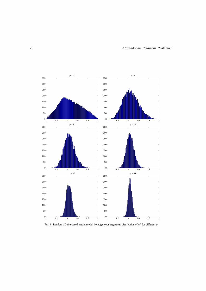
We consider a random structure where the conductivity profile for each tiley ∈ Y is the constantfunction given byfy(τ) = y for all τ ∈ Tor

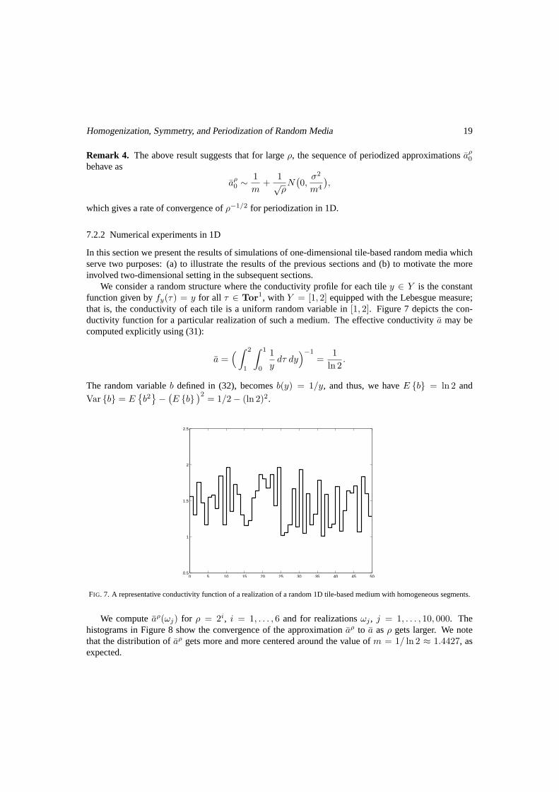
1, with Y = [1, 2] equipped with the Lebesgue measure;that is, the conductivity of each tile is a uniform random variable in [1, 2]. Figure 7 depicts the con-ductivity function for a particular realization of such a medium. The effective conductivitya may becomputed explicitly using (31):

a =(

∫ 2

1

∫ 1

0

1

ydτ dy

)−1

=1

ln 2.

The random variableb defined in (32), becomesb(y) = 1/y, and thus, we haveE b = ln 2 and

Var b = E

b2

−(

E b)2

= 1/2− (ln 2)2.

0 5 10 15 20 25 30 35 40 45 500.5

1

1.5

2

2.5

FIG. 7. A representative conductivity function of a realization of a random 1D tile-based medium with homogeneous segments.

We computeaρ(ωj) for ρ = 2i, i = 1, . . . , 6 and for realizationsωj , j = 1, . . . , 10, 000. Thehistograms in Figure 8 show the convergence of the approximation aρ to a asρ gets larger. We notethat the distribution ofaρ gets more and more centered around the value ofm = 1/ ln 2 ≈ 1.4427, asexpected.


1 1.2 1.4 1.6 1.8 20

50

100

150

200

250

300

350ρ = 2

1 1.2 1.4 1.6 1.8 20

50

100

150

200

250

300

350ρ = 4

1 1.2 1.4 1.6 1.8 20

50

100

150

200

250

300

350ρ = 8

1 1.2 1.4 1.6 1.8 20

50

100

150

200

250

300

350ρ = 16

1 1.2 1.4 1.6 1.8 20

50

100

150

200

250

300

350ρ = 32

1 1.2 1.4 1.6 1.8 20

50

100

150

200

250

300

350ρ = 64

FIG. 8. Random 1D tile-based medium with homogeneous segments: distribution of aρ for differentρ


ρ Mean Variance σ2

m4ρRatio

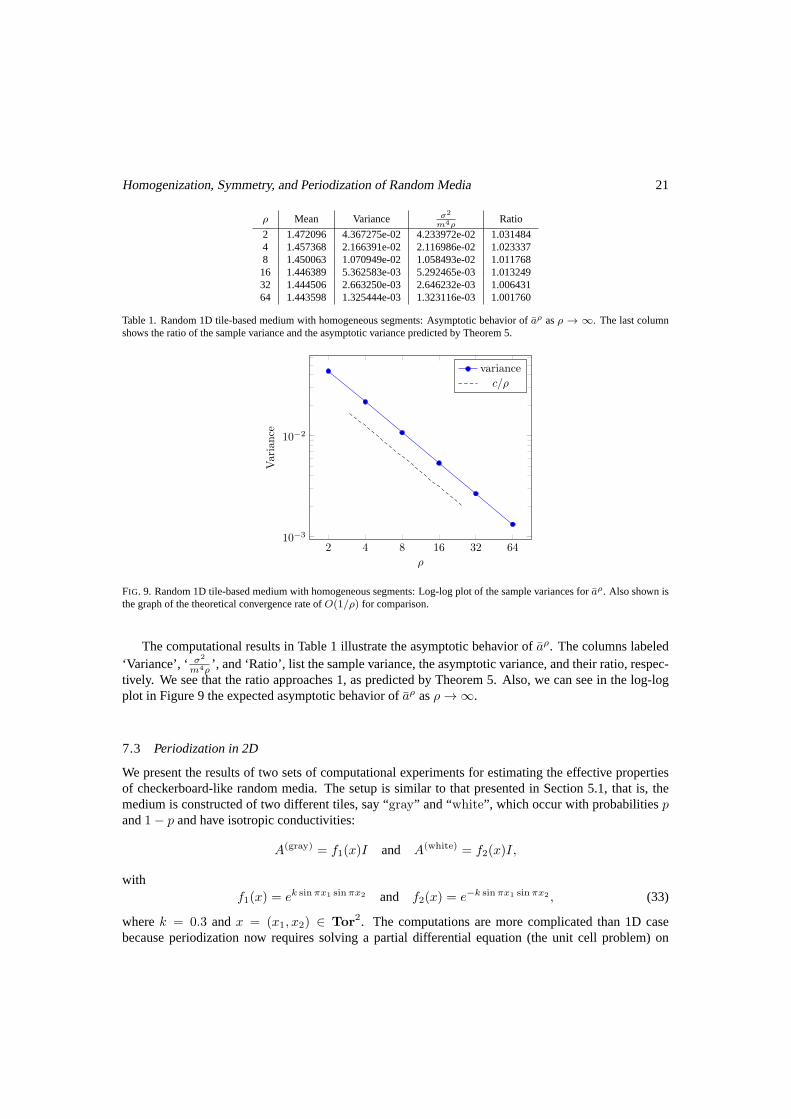
2 1.472096 4.367275e-02 4.233972e-02 1.0314844 1.457368 2.166391e-02 2.116986e-02 1.0233378 1.450063 1.070949e-02 1.058493e-02 1.01176816 1.446389 5.362583e-03 5.292465e-03 1.01324932 1.444506 2.663250e-03 2.646232e-03 1.00643164 1.443598 1.325444e-03 1.323116e-03 1.001760

Table 1. Random 1D tile-based medium with homogeneous segments: Asymptotic behavior ofaρ asρ → ∞. The last columnshows the ratio of the sample variance and the asymptotic variance predicted by Theorem 5.

2 4 8 16 32 6410

−3

10−2

ρ

Varia

nce

variance

c/ρ

FIG. 9. Random 1D tile-based medium with homogeneous segments: Log-log plot of the sample variances foraρ. Also shown isthe graph of the theoretical convergence rate ofO(1/ρ) for comparison.

The computational results in Table 1 illustrate the asymptotic behavior ofaρ. The columns labeled‘Variance’, ‘ σ2

m4ρ ’, and ‘Ratio’, list the sample variance, the asymptotic variance, and their ratio, respec-tively. We see that the ratio approaches 1, as predicted by Theorem 5. Also, we can see in the log-logplot in Figure 9 the expected asymptotic behavior ofaρ asρ → ∞.

7.3 Periodization in 2D

We present the results of two sets of computational experiments for estimating the effective propertiesof checkerboard-like random media. The setup is similar to that presented in Section 5.1, that is, themedium is constructed of two different tiles, say “gray” and “white”, which occur with probabilitiespand1− p and have isotropic conductivities:

A(gray) = f1(x)I and A(white) = f2(x)I,

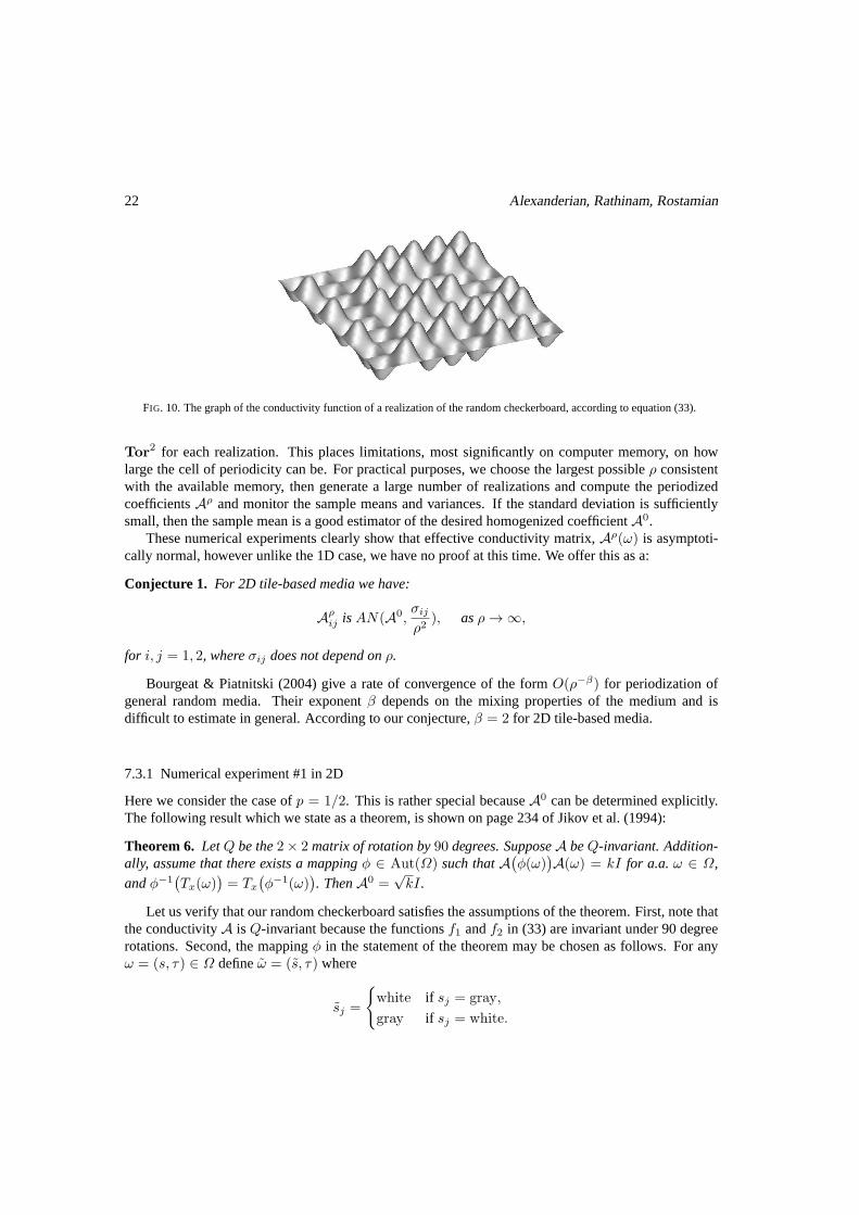
withf1(x) = ek sinπx1 sinπx2 and f2(x) = e−k sinπx1 sinπx2 , (33)

wherek = 0.3 andx = (x1, x2) ∈ Tor2. The computations are more complicated than 1D case

because periodization now requires solving a partial differential equation (the unit cell problem) on


FIG. 10. The graph of the conductivity function of a realizationof the random checkerboard, according to equation (33).

Tor2 for each realization. This places limitations, most significantly on computer memory, on how

large the cell of periodicity can be. For practical purposes, we choose the largest possibleρ consistentwith the available memory, then generate a large number of realizations and compute the periodizedcoefficientsAρ and monitor the sample means and variances. If the standard deviation is sufficientlysmall, then the sample mean is a good estimator of the desiredhomogenized coefficientA0.

These numerical experiments clearly show that effective conductivity matrix,Aρ(ω) is asymptoti-cally normal, however unlike the 1D case, we have no proof at this time. We offer this as a:

Conjecture 1. For 2D tile-based media we have:

Aρij is AN(A0,

σij

ρ2), asρ → ∞,

for i, j = 1, 2, whereσij does not depend onρ.

Bourgeat & Piatnitski (2004) give a rate of convergence of the formO(ρ−β) for periodization ofgeneral random media. Their exponentβ depends on the mixing properties of the medium and isdifficult to estimate in general. According to our conjecture,β = 2 for 2D tile-based media.

7.3.1 Numerical experiment #1 in 2D

Here we consider the case ofp = 1/2. This is rather special becauseA0 can be determined explicitly.The following result which we state as a theorem, is shown on page 234 of Jikov et al. (1994):

Theorem 6. LetQ be the2× 2 matrix of rotation by90 degrees. SupposeA beQ-invariant. Addition-ally, assume that there exists a mappingφ ∈ Aut(Ω) such thatA

(

φ(ω))

A(ω) = kI for a.a.ω ∈ Ω,

andφ−1(

Tx(ω))

= Tx

(

φ−1(ω))

. ThenA0 =√kI.

Let us verify that our random checkerboard satisfies the assumptions of the theorem. First, note thatthe conductivityA is Q-invariant because the functionsf1 andf2 in (33) are invariant under 90 degreerotations. Second, the mappingφ in the statement of the theorem may be chosen as follows. For anyω = (s, τ) ∈ Ω defineω = (s, τ) where

sj =

white if sj = gray,

gray if sj = white.


[Aρ]11 [Aρ]22

ρ Mean Variance Ratio2 0.99939138 3.87392708e-03 —4 0.99900417 8.29923510e-04 4.66788 0.99972096 2.15407332e-04 3.852816 0.99974253 5.64378707e-05 3.816732 1.00003515 1.46838211e-05 3.843564 0.99997816 3.62430817e-06 4.0515


[Aρ]12 [Aρ]21

ρ Mean Variance Ratio2 0.00000000 0.00000000e+00 —4 -0.00001521 5.17427142e-07 0.00008 -0.00001938 2.21103369e-07 2.340216 -0.00000147 6.44481557e-08 3.430732 -0.00000278 1.63013662e-08 3.953564 -0.00000056 4.11889874e-09 3.9577

ρ Mean Variance Ratio2 0.00000000 0.00000000e+00 —4 -0.00001521 5.17427142e-07 0.00008 -0.00001938 2.21103369e-07 2.340216 -0.00000147 6.44481557e-08 3.430732 -0.00000278 1.63013662e-08 3.953564 -0.00000056 4.11889874e-09 3.9577

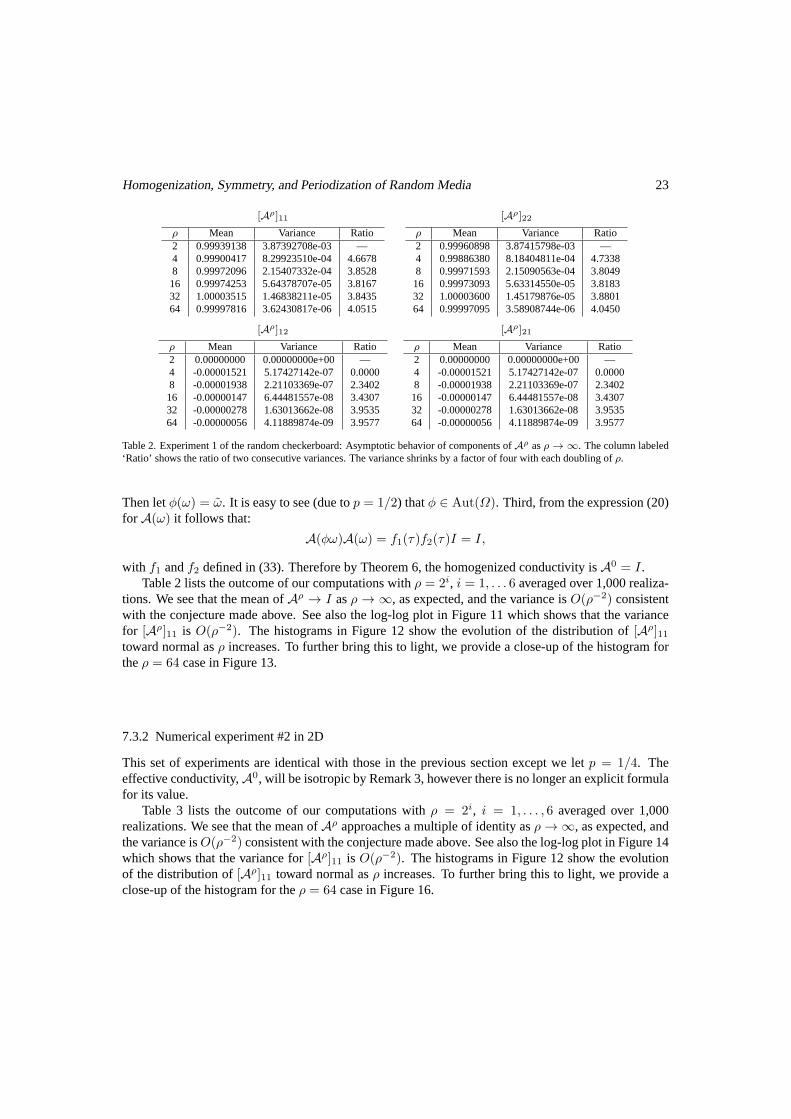
Table 2. Experiment 1 of the random checkerboard: Asymptotic behavior of components ofAρ asρ → ∞. The column labeled‘Ratio’ shows the ratio of two consecutive variances. The variance shrinks by a factor of four with each doubling ofρ.

Then letφ(ω) = ω. It is easy to see (due top = 1/2) thatφ ∈ Aut(Ω). Third, from the expression (20)for A(ω) it follows that:

A(φω)A(ω) = f1(τ)f2(τ)I = I,

with f1 andf2 defined in (33). Therefore by Theorem 6, the homogenized conductivity isA0 = I.Table 2 lists the outcome of our computations withρ = 2i, i = 1, . . . 6 averaged over 1,000 realiza-

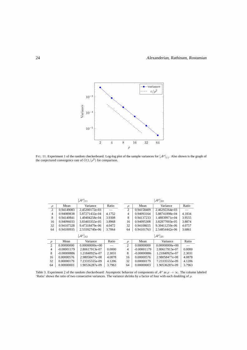
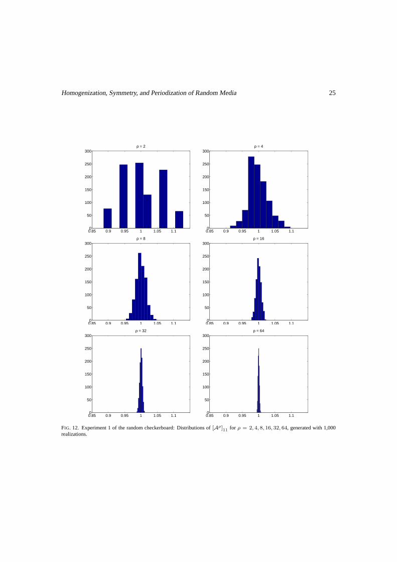
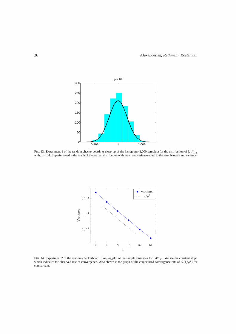
tions. We see that the mean ofAρ → I asρ → ∞, as expected, and the variance isO(ρ−2) consistentwith the conjecture made above. See also the log-log plot in Figure 11 which shows that the variancefor [Aρ]11 is O(ρ−2). The histograms in Figure 12 show the evolution of the distribution of [Aρ]11toward normal asρ increases. To further bring this to light, we provide a close-up of the histogram fortheρ = 64 case in Figure 13.

7.3.2 Numerical experiment #2 in 2D

This set of experiments are identical with those in the previous section except we letp = 1/4. Theeffective conductivity,A0, will be isotropic by Remark 3, however there is no longer an explicit formulafor its value.

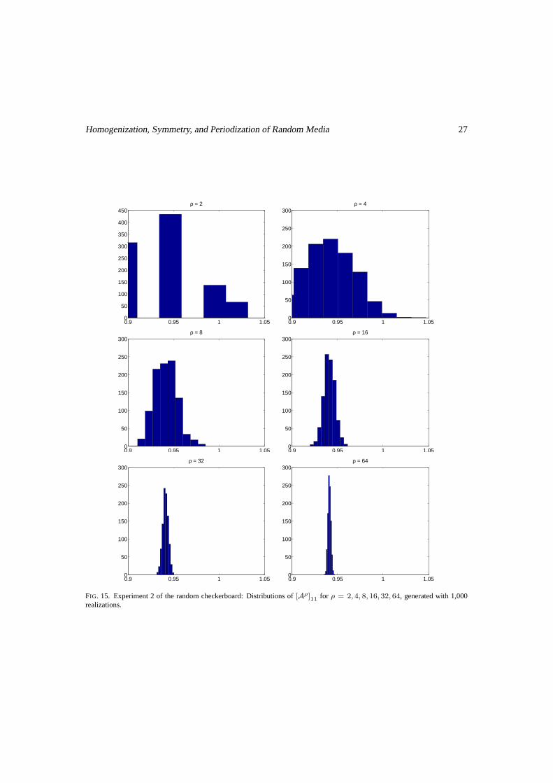
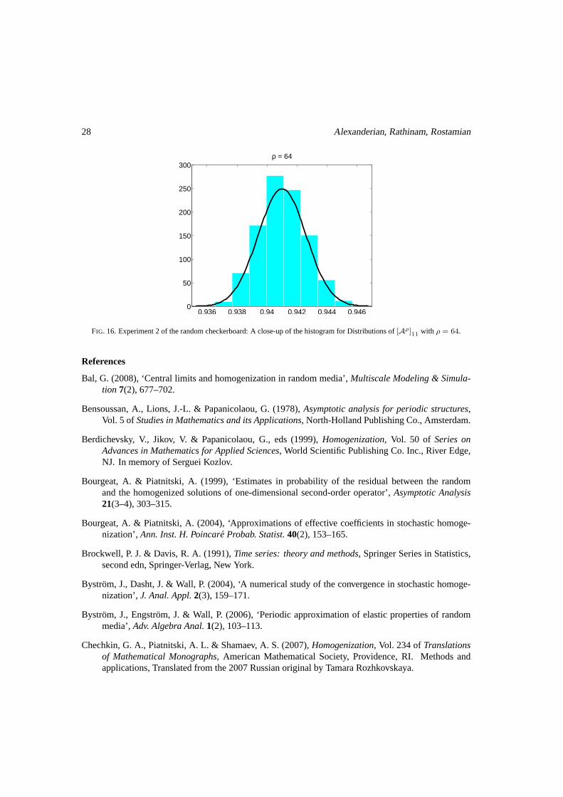
Table 3 lists the outcome of our computations withρ = 2i, i = 1, . . . , 6 averaged over 1,000realizations. We see that the mean ofAρ approaches a multiple of identity asρ → ∞, as expected, andthe variance isO(ρ−2) consistent with the conjecture made above. See also the log-log plot in Figure 14which shows that the variance for[Aρ]11 is O(ρ−2). The histograms in Figure 12 show the evolutionof the distribution of[Aρ]11 toward normal asρ increases. To further bring this to light, we provide aclose-up of the histogram for theρ = 64 case in Figure 16.


2 4 8 16 32 64

10−5

10−4

10−3

ρ

Variance

variance

c/ρ2

FIG. 11. Experiment 1 of the random checkerboard: Log-log plot ofthe sample variances for[Aρ]11

. Also shown is the graph ofthe conjectured convergence rate ofO(1/ρ2) for comparison.

[Aρ]11 [Aρ]22



[Aρ]12 [Aρ]21

ρ Mean Variance Ratio2 0.00000000 0.00000000e+00 —4 -0.00001179 2.80617913e-07 0.00008 -0.00000886 1.21840925e-07 2.303116 0.00000576 2.98058477e-08 4.087832 0.00000179 7.23335555e-09 4.120664 0.00000003 1.90536287e-09 3.7963

ρ Mean Variance Ratio2 0.00000000 0.00000000e+00 —4 -0.00001179 2.80617913e-07 0.00008 -0.00000886 1.21840925e-07 2.303116 0.00000576 2.98058477e-08 4.087832 0.00000179 7.23335555e-09 4.120664 0.00000003 1.90536287e-09 3.7963

Table 3. Experiment 2 of the random checkerboard: Asymptotic behavior of components ofAρ asρ → ∞. The column labeled‘Ratio’ shows the ratio of two consecutive variances. The variance shrinks by a factor of four with each doubling ofρ.


0.85 0.9 0.95 1 1.05 1.10

50

100

150

200

250

300ρ = 2

0.85 0.9 0.95 1 1.05 1.10

50

100

150

200

250

300ρ = 4

0.85 0.9 0.95 1 1.05 1.10

50

100

150

200

250

300ρ = 8

0.85 0.9 0.95 1 1.05 1.10

50

100

150

200

250

300ρ = 16

0.85 0.9 0.95 1 1.05 1.10

50

100

150

200

250

300ρ = 32

0.85 0.9 0.95 1 1.05 1.10

50

100

150

200

250

300ρ = 64

FIG. 12. Experiment 1 of the random checkerboard: Distributionsof [Aρ]11

for ρ = 2, 4, 8, 16, 32, 64, generated with 1,000realizations.


0.995 1 1.0050

50

100

150

200

250

300ρ = 64

FIG. 13. Experiment 1 of the random checkerboard: A close-up of the histogram (1,000 samples) for the distribution of[Aρ]11

with ρ = 64. Superimposed is the graph of the normal distribution with meanand variance equal to the sample mean and variance.

2 4 8 16 32 64

10−5

10−4

10−3

ρ

Variance

variance

c/ρ2

FIG. 14. Experiment 2 of the random checkerboard: Log-log plot ofthe sample variances for[Aρ]11

. We see the constant slopewhich indicates the observed rate of convergence. Also shown is the graph of the conjectured convergence rate ofO(1/ρ2) forcomparison.


0.9 0.95 1 1.050

50

100

150

200

250

300

350

400

450ρ = 2

0.9 0.95 1 1.050

50

100

150

200

250

300ρ = 4

0.9 0.95 1 1.050

50

100

150

200

250

300ρ = 8

0.9 0.95 1 1.050

50

100

150

200

250

300ρ = 16

0.9 0.95 1 1.050

50

100

150

200

250

300ρ = 32

0.9 0.95 1 1.050

50

100

150

200

250

300ρ = 64

FIG. 15. Experiment 2 of the random checkerboard: Distributionsof [Aρ]11

for ρ = 2, 4, 8, 16, 32, 64, generated with 1,000realizations.


0.936 0.938 0.94 0.942 0.944 0.9460

50

100

150

200

250

300ρ = 64

FIG. 16. Experiment 2 of the random checkerboard: A close-up of the histogram for Distributions of[Aρ]11

with ρ = 64.

References

Bal, G. (2008), ‘Central limits and homogenization in random media’,Multiscale Modeling & Simula-tion 7(2), 677–702.

Bensoussan, A., Lions, J.-L. & Papanicolaou, G. (1978),Asymptotic analysis for periodic structures,Vol. 5 of Studies in Mathematics and its Applications, North-Holland Publishing Co., Amsterdam.

Berdichevsky, V., Jikov, V. & Papanicolaou, G., eds (1999),Homogenization, Vol. 50 of Series onAdvances in Mathematics for Applied Sciences, World Scientific Publishing Co. Inc., River Edge,NJ. In memory of Serguei Kozlov.

Bourgeat, A. & Piatnitski, A. (1999), ‘Estimates in probability of the residual between the randomand the homogenized solutions of one-dimensional second-order operator’,Asymptotic Analysis21(3–4), 303–315.

Bourgeat, A. & Piatnitski, A. (2004), ‘Approximations of effective coefficients in stochastic homoge-nization’,Ann. Inst. H. Poincare Probab. Statist.40(2), 153–165.

Brockwell, P. J. & Davis, R. A. (1991),Time series: theory and methods, Springer Series in Statistics,second edn, Springer-Verlag, New York.

Bystrom, J., Dasht, J. & Wall, P. (2004), ‘A numerical study of the convergence in stochastic homoge-nization’,J. Anal. Appl.2(3), 159–171.

Bystrom, J., Engstrom, J. & Wall, P. (2006), ‘Periodic approximation of elasticproperties of randommedia’,Adv. Algebra Anal.1(2), 103–113.

Chechkin, G. A., Piatnitski, A. L. & Shamaev, A. S. (2007),Homogenization, Vol. 234 ofTranslationsof Mathematical Monographs, American Mathematical Society, Providence, RI. Methods andapplications, Translated from the 2007 Russian original byTamara Rozhkovskaya.


Cioranescu, D. & Donato, P. (1999),An introduction to homogenization, Vol. 17 of Oxford LectureSeries in Mathematics and its Applications, The Clarendon Press Oxford University Press, NewYork.

Cornfeld, I. P., Fomin, S. V. & Sinaı, Y. G. (1982),Ergodic theory, Vol. 245 ofGrundlehren der Math-ematischen Wissenschaften [Fundamental Principles of Mathematical Sciences], Springer-Verlag,New York. Translated from the Russian by A. B. Sosinskiı.

Efendiev, Y. & Pankov, A. (2004a), ‘Numerical homogenization and correctors for nonlinearellipticequations’,SIAM J. Appl. Math.65(1), 43–68 (electronic).

Efendiev, Y. & Pankov, A. (2004b), ‘Numerical homogenization of nonlinear random parabolic opera-tors’, Multiscale Model. Simul.2(2), 237–268 (electronic).

Fulton, W. & Harris, J. (1991),Representation theory, Vol. 129 of Graduate Texts in Mathematics,Springer-Verlag, New York.

James, G. & Liebeck, M. (2001),Representations and characters of groups, second edn, CambridgeUniversity Press, New York.

Jikov, V. V., Kozlov, S. M. & Oleınik, O. A. (1994),Homogenization of differential operators andintegral functionals, Springer-Verlag, Berlin. Translated from the Russian by G. A. Yosifian [G.A. Iosif′yan].

Kozlov, S. M. (1979), ‘The averaging of random operators’,Mat. Sb. (N.S.)109(151)(2), 188–202, 327.

Oleınik, O. A., Shamaev, A. S. & Yosifian, G. A. (1992),Mathematical problems in elasticity andhomogenization, Vol. 26 ofStudies in Mathematics and its Applications, North-Holland PublishingCo., Amsterdam.

Owhadi, H. (2003), ‘Approximation of the effective conductivity of ergodic media by periodization’,Probab. Theory Related Fields125(2), 225–258.

Pankov, A. (1997),G-convergence and homogenization of nonlinear partial differential operators, Vol.422 ofMathematics and its Applications, Kluwer Academic Publishers, Dordrecht.

Papanicolaou, G. C. (1995), Diffusion in random media,in J. B. Keller, D. McLaughlin & G. C. Pa-panicolaou, eds, ‘Surveys in applied mathematics, Vol. 1’,Vol. 1 of Surveys Appl. Math., Plenum,New York, pp. 205–253.

Papanicolaou, G. C. & Varadhan, S. R. S. (1981), Boundary value problems with rapidly oscillatingrandom coefficients,in ‘Random fields, Vol. I, II (Esztergom, 1979)’, Vol. 27 ofColloq. Math.Soc. Janos Bolyai, North-Holland, Amsterdam, pp. 835–873.

Sab, K. (1992), ‘On the homogenization and the simulation ofrandom materials’,European J. Mech. ASolids11(5), 585–607.

Sanchez-Palencia, E. (1980),Nonhomogeneous media and vibration theory, Vol. 127 ofLecture Notesin Physics, Springer-Verlag, Berlin.

Schur, I. (1905), ‘Neue begrundung der theorie der gruppencharaktere’,Sitzungsberichte der KoniglichPreußischen Akademie der Wissenschaften zu Berlin, Part 1pp. 406–432.


Telega, J. J. & Bielski, W. (2002), ‘Stochastic homogenization and macroscopic modelling of compos-ites and flow through porous media’,Theoret. Appl. Mech.28/29, 337–377. Issue dedicated to thememory of Professor Rastko Stojanovic (Belgrade, 2002).

Walters, P. (1982),An introduction to ergodic theory, Vol. 79 of Graduate Texts in Mathematics,Springer-Verlag, New York.

Weyl, H. (1946),The classical groups, Princeton Landmarks in Mathematics, Princeton UniversityPress, Princeton, NJ. Their invariants and representations, 2nd Edition.

Williams, D. (1991),Probability with martingales, Cambridge Mathematical Textbooks, CambridgeUniversity Press, Cambridge.

Wu, X. H., Efendiev, Y. & Hou, T. Y. (2002), ‘Analysis of upscaling absolute permeability’,DiscreteContin. Dyn. Syst. Ser. B2(2), 185–204.

Yue, X. & E, W. (2007), ‘The local microscale problem in the multiscale modeling of strongly hetero-geneous media: Effects of boundary conditions and cell size’, Journal of Computational Physics222(2), 556–572.

Zhikov, V. V. & Pyatnitskiı, A. L. (2006), ‘Homogenization of random singular structures and randommeasures’,Izvestiya. Mathematics70(1), 19–67.

Documents

Homogenization, Symmetry, and Periodization in …aalexan3/articles/homog-paper.pdf · Homogenization, Symmetry, and Periodization in Diffusive Random ... Lions & Papanicolaou