Homo Moralis

–

preference evolution under incomplete

information and assortative matching∗

Ingela Alger† and Jörgen W. Weibull‡

March 1, 2012

Abstract

What preferences will prevail in a society of rational individuals when preference

evolution is driven by their success in terms of resulting payoffs? We show that when

individuals’ preferences are their private information, a convex combinations of self-

ishness and morality stand out as evolutionarily stable. We call individuals with such

preferences homo moralis. At one end of the spectrum is homo oeconomicus, who acts

so as to maximize his or her material payoff. At the opposite end is homo kantiensis,

who does what would be “the right thing to do,” in terms of material payoffs, if all

others would do likewise. We show that the stable degree of morality - the weight

placed on the moral goal - equals the index of assortativity in the matching process.

The motivation of homo moralis is arguably compatible with how people often reason,

and the induced behavior appear to agree with pro-social behaviors observed in many

laboratory experiments.

Keywords: evolutionary stability, preference evolution, moral values, incomplete

information, assortative matching.

JEL codes: C73, D03.

∗An early version of this paper was presented at the NBER workshop on culture and institutions in

November 2011. We thank Rajiv Sethi for helpful comments to that version. We also thank Immanuel

Bomze, Avinash Dixit, Tore Ellingsen, Jens Josephson, Klaus Ritzberger, François Salanié, and Giancarlo

Spagnolo for comments. This research received financial support from the Knut and Alice Wallenberg

Research Foundation. Ingela Alger is grateful to Carleton University and SSHRC for financial support and

to the Stockholm School of Economics for its hospitality.

†LERNA/CNRS @ Toulouse School of Economics, and Carleton University (Ottawa)

‡Stockholm School of Economics, École Polytechnique (Paris), and Royal Institute of Technology (Stock-

holm)

1

1 Introduction

Most of contemporary economics is premised on the assumption that human behavior is

driven by self-interest. This assumption provides predictive power in many areas of eco-

nomics. Moreover, economists have used it to identify conditions under which self-interest

leads to the common good. However, in the early history of the profession, it was common to

include moral values in human motivation, see e.g. Smith (1759) and Edgeworth (1881), and

for more recent examples, Arrow (1973), Laffont (1975), Sen (1977), and Tabellini (2008).1

Moreover, in recent years many economists, particularly within behavioral and experimental

economics, have begun to question the predictive power of pure selfishness in certain inter-

actions and turned to social, or “other-regarding” preferences. Our goal is here to clarify

the evolutionary foundation of human motivation. Like many others before us, but now in a

more general setting, we investigate whether pure self-interest is favored by evolution. With

virtually no restrictions on the class of potential preferences that may be selected for, our

main result is that natural selection leads to a certain one-dimensional spectrum of moral

preferences, a spectrum that sprang out from the mathematics. At one end of this spectrum

is pure self-interest and at the other is pure ethical reasoning in line with Kant’s categorical

imperative.

It is well-known that it may be advantageous in strategic interactions to be commit-

ted to certain behaviors, even if these appear to be at odds with one’s objective self-interest

(Schelling, 1960). Likewise, certain other-regarding preferences such as altruism, spite, recip-

rocal altruism, or inequity aversion, if known or believed by others, may be strategically

advantageous (or disadvantageous). For example, a proposer in ultimatum bargaining may

be more generous if the responder is known or believed to be inequity averse rather than

solely interested in own monetary gains. This raises the further question whether evolution

would favor such preferences.

In the literature addressing this issue, usually called the indirect evolutionary approach,

pioneered by Güth and Yaari (1992), much work has been devoted to the case where individ-

uals are uniformly randomly matched and know each others’ preferences.2 Usually, evolution

then favors other preferences than those of homo oeconomicus (see Heifetz, Shannon, and

Spiegel, 2007, for a particularly general such result). By contrast, when individuals are uni-

formly randomly matched and preferences are private information, evolution leads to the

self-interested homo oeconomicus, see Ok and Vega-Redondo (2001), and Dekel, Ely and

Yilankaya (2007). We here propose a theory for why evolution may lead to preferences that

1See Binmore (1994) for a game-theoretic discussion of ethics.

2See Frank (1987), Robson (1990), Güth and Yaari (1992), Ellingsen (1997), Bester and Güth (1998),

Fershtman and Weiss (1998), Koçkesen, Ok and Sethi (2000), Bolle (2000), Possajennikov (2000), Ok and

Vega-Redondo (2001), Sethi and Somanathan (2001), Heifetz, Shannon and Spiegel (2006, 2007), Dekel, Ely

and Yilankaya (2007), Alger and Weibull (2010, 2011), and Alger (2010).

2

differ from those of homo oeconomicus even when preferences are private information. The

reason for our different result is that we permit assortativity in the matching process that

brings individuals together.

More exactly, we analyze the evolution of preferences in a large population where individ-

uals are randomly and pairwise matched to interact. In each interaction, individual behavior

is driven by (subjective) utility maximization, while evolutionary success is driven by some

(objective) payoff. The key element in our theory is that the matching process may be more

or less assortative, that is, individuals with the same preferences may be more or less likely

to be matched with each other. Such assortativity arises as soon as there is some probability

that the individuals inherited their preferences from some common ancestor (be it a genetic

or a cultural ancestor). Assortativity is arguably common, because of a tendency to inter-

act with kin, with people in the same geographical area or from the same school, or with

people with the same culture, religion, or values (see e.g. Eshel and Cavalli-Sforza, 1982).

By contrast, existing models of preference evolution assume that individuals are uniformly

randomly matched.3 The matching process is here exogenous, and, building on Bergstrom

(2003), we identify a single parameter, the index of assortativity, as a key parameter for the

population-statistical analysis. We generalize the definition of evolutionary stability to allow

for arbitrary degrees of assortativity in the matching process, and apply this to preference

evolution when each matched pair plays a (Bayesian) Nash equilibrium of the associated

game under incomplete information, that is, as if they each knew the statistical preference

distribution in their matches, but not the preferences of the other individual in the match

at hand.

With a minimum of additional assumptions, this leads to a remarkable result: a certain

convex combination of selfishness – “maximization of own payoff” – and a certain form

of morality –“to do what would lead to maximal payoff if everybody else did likewise” –

stands out as evolutionarily stable. Individuals with preferences in this one-dimensional class

will be called homo moralis and the weight attached to the moral goal the degree of morality.

A special case is the familiar homo oeconomicus, whose utility function coincides with the

objective payoff function. At the other extreme one finds homo kantiensis, who strives to

maximize the payoff that would result should everybody behave in the same way.

Our main finding is that evolution selects that degree of morality which equals the index

of assortativity in the matching process. In a resident population, such preferences turn out

to provide the most effective protection against rare mutants, since they induce their carriers

to behave in such a way that the same behavior is then also payoff-optimal for rare mutants,

should such appear. Hence, it is as if moral preferences with the right weight attached to

the moral goal preempt mutants; a rare mutant can at best match the payoff of the resident

population.

3Exceptions are Alger and Weibull (2010, 2011) and Alger (2010).

3

This result has dire consequences for homo oeconomicus in many situations. In particular,

homo oeconomicus is selected against as soon as an individual’s payoff depends on the other’s

action and the matching process has a positive index of assortativity. Arguably, these two

features are common, implying that we should expect a positive degree of morality, rather

than the pure selfishness of homo oeconomicus, to prevail in many settings.

It is beyond the scope of this paper to provide a comprehensive analysis of the behavior

of homo moralis. It is not difficult to show, however, that homo moralis’ behavior in in-

teractions commonly studied in laboratory experiments is compatible with observation (as

reported in, e.g., Fehr and Gächter, 2000, Gächter, Herrmann and Thöni, 2004, Henrich

et al., 2005, and Gächter and Herrmann, 2009). In particular, homo moralis gives positive

amounts in dictator games, may reject positive amounts in ultimatum games, and contributes

more to public goods than would be motivated by material self-interest.4 For further analy-

ses of the behavioral implications of preferences similar to those of homo moralis, see Laffont

(1975), Brekke, Kverndokk, and Nyborg (2003), and Huck, Kübler and Weibull (2011).5

As a side result, we obtain a new interpretation of evolutionary stability of strategies

(here under random matching with arbitrary degree of assortativity), namely, that these are

precisely the behaviors one will observe in Nash equilibrium play under incomplete informa-

tion, when evolution operates at the level of preferences, rather than directly on strategies.

This sharpens and generalizes the result in Dekel et al. (2007) that preference evolution un-

der incomplete information and uniform random matching in finite games implies symmetric

Nash equilibrium play and is implied by strict symmetric Nash equilibrium play (in both

cases with Nash equilibrium defined in terms of payoffs).

The model is set up in the next section. In Section 3 we establish our main result and

show some of its implications. Section 4 is devoted to finite games. In Section 5 we study a

variety of matching processes. Section 6 discusses related literature, morality and altruism,

and empirical testing. Section 7 concludes.

2 The model

Consider a population where individuals are matched into pairs to engage in a symmetric

interaction with the common strategy set, . While behavior is driven by (subjective) utility

maximization, evolutionary success is determined by the resulting payoffs. An individual

playing strategy against an individual playing strategy gets payoff, or fitness increment,

( ), where : 2 → R. We will refer to the pair hi as the fitness game. We assume

4We refer to the working paper version for this analysis. Furthermore, in Section 6 we provide a suggestion

for an experimental design.

5See Bacharach (1999) for “team reasoning” and Roemer (2010) for an approach to “Kantian equilibrium.”

4

that is a non-empty, compact and convex set in a topological vector space, and that

is continuous.6 Each individual is characterized by his or her type ∈ Θ, which defines a

continuous utility function, : 2 → R. We impose no mathematical relation between a

utility function and the payoff function . A special type is homo oeconomicus, by which

we mean individuals with the special utility function = .

For the subsequent analysis, it will be sufficient to consider populations with at most

two types present. The two types and the respective population shares together define

a population state = ( ), where ∈ Θ are the two types and ∈ [0 1] is thepopulation share of type .7 If is small we will refer to as the resident type, and call

the mutant type. The set of population states is thus = Θ2 × [0 1].The matching process is random and exogenous, but we allow it to be assortative. More

exactly, in a given state = ( ), let Pr [ | ] denote the probability that a given indi-vidual of type will be matched with an individual of type , and Pr [| ] the probabilitythat a given individual of type will be matched with an individual of type . In the special

case of uniform random matching, Pr [ | ] = Pr [ | ] = .

For each state = ( ) ∈ , and any strategy ∈ used by type and any strategy

∈ used by type , the resulting average payoff, or fitness, to the two types are:

( ) = Pr [| ] · ( ) + Pr [ | ] · ( ) (1)

( ) = Pr [| ] · ( ) + Pr [ | ] · ( ) (2)

Turning now to the choices made by individuals in a population state, we define (Bayesian)

Nash equilibrium as a pair of strategies, one for each type, where each strategy is a best

reply to the other in the given population state:

Definition 1 In any state = ( ) ∈ , a strategy pair (∗ ∗) ∈ 2 is a (Bayesian)

Nash Equilibrium (BNE) if½∗ ∈ argmax∈ Pr [| ] · ( ∗) + Pr [ | ] · ( ∗)∗ ∈ argmax∈ Pr [| ] · ( ∗) + Pr [ | ] · ( ∗) (3)

Evolutionary stability is defined under the assumption that the resulting payoffs are

determined by this equilibrium set. With potential multiplicity of equilibria, one may require

the resident type to withstand invasion in some or all equilibria. We have chosen the most

severe criterion.8

6To be more precise, we assume to be a locally convex Hausdorff space, see Aliprantis and Border

(2006). The subsequent examples are all carried out in the special but important case of Euclidean spaces.

7In particular, in the population state = ( 0) only type is present.

8The least stringent criterion would be to replace “all Nash equilibria” by “some Nash equilibrium.”

5

Definition 2 A type ∈ Θ is evolutionarily stable against a type ∈ Θ if there exists

an 0 such that (∗ ∗ ) (

∗ ∗ ) in all Nash equilibria (∗ ∗) in all states = ( ) with ∈ (0 ). A type is evolutionarily stable if it is evolutionarily stableagainst all types 6= in Θ.

This definition formalizes the notion that a resident population with individuals of a given

type would withstand a small-scale “invasion” of individuals of another type. It generalizes

the Maynard Smith and Price (1973) concept of an evolutionarily stable strategy, a property

they defined for mixed strategies in finite and symmetric two-player games under uniform

random matching.

In a rich enough type spaceΘ, no type is evolutionarily stable, since for each resident type

there then exist mutant types who respond with the same strategy, in which case both

types earn the same average payoff. However, many types will turn out to be vulnerable, as

residents, to invasion by better-performing mutant types. We will use the following definition

to describe this possibility:

Definition 3 A type ∈ Θ is evolutionarily unstable if there exists a type ∈ Θ such

that for each 0 there exists an ∈ (0 ) such that (∗ ∗ ) (

∗ ∗ ) in allNash equilibria (∗ ∗) in state = ( ).

This is also a stringent criterion, namely, there should exist some mutant type against

which the resident type achieves less payoff in every equilibrium in some population states

when the mutant is arbitrarily rare.

This completes the description of the model. The most closely related work on preference

evolution under incomplete information, Ok and Vega-Redondo (2001), or OVR for short,

and Dekel, Ely and Yilankaya (2007), or DEY for short. In all three models, the preference

space is very general and interactions are symmetric. In OVR the population is finite whereas

in DEY and our model it is a continuum. In OVR each interaction may involve more than two

individuals, whereas in DEY and our model interactions are pairwise. In OVR, individual

use pure strategies, the pure-strategy set is a continuum and the payoff function is strictly

concave, whereas DEY focus on mixed strategies in finite games. We analyze both cases and

do not require strict concavity. All three papers study evolutionary stability, although the

definitions differ slightly from one another. A key difference between our model and OVR

and DEY is that they assume uniform random matching, whereas we allow for assortative

matching.

The next subsection describes the algebra of assortative encounters introduced by Bergstrom

(2003). This algebra facilitates the analysis and clarifies the population-statistical aspects.

6

2.1 Algebra of assortative encounters

For given types ∈ Θ, and a population state = ( ) with ∈ (0 1), let () bethe difference between the conditional probabilities for an individual to be matched with an

individual with type , given that the individual him- or herself either also has type , or,

alternatively, type :

() = Pr [| ]− Pr [| ] (4)

This defines the assortment function : (0 1) → [−1 1]. Using the following necessarybalancing condition for the number of pairwise matches between individuals with types

and ,

(1− ) · [1− Pr [| ]] = · Pr [| ] (5)

one can write both conditional probabilities as functions of and ():½Pr [| ] = () + (1− ) [1− ()]

Pr [| ] = (1− ) [1− ()] (6)

We assume that is continuous and that () converges to some number as tends to zero.

Formally:

lim→0

() =

for some ∈ R, the index of assortativity of the matching process. This extends the domainof from (0 1) to [0 1], and it follows from (6) that ∈ [0 1]. The extreme case = 0

corresponds to uniform random matching and the opposite extreme case = 1 to perfectly

correlated matching (each type only meets itself). In Section 5 we calculate the index of

assortativity for a variety of matching processes.

2.2 Homo moralis

Definition 4 An individual is a homo moralis (or HM) if her utility function is of the

form

( ) = (1− ) · ( ) + · ( ) (7)

for some ∈ [0 1], the degree of morality.9

It is as if homo moralis is torn between selfishness and morality. On the one hand, she

would like to maximize her own payoff, ( ). On the other hand, she would like to “do

the right thing” in terms of payoffs, i.e., choose a strategy that would be optimal, in terms

of the payoff, if both players would choose one and the same strategy. This second goal can

9We thus adopt the notational convention that types that are real numbers in the unit interval refer to

homo moralis with that degree of morality.

7

be viewed as an application of Kant’s categorical imperative to the goal of enhancement of

everyone’s (objective) payoff (or fitness).10 Torn by these two goals, homo moralis will take

an action that maximizes a convex combination of them.11 If = 0, the definition of homo

moralis coincides with that of homo oeconomicus.

Remark 1 It is clear from (7) that the behavior of homo moralis is unaffected by positive

affine transformations of payoffs. However, if and are mixed strategies (say, in a finite

game), then the preferences of homo moralis, for 0, are not linear, but quadratic, in the

own mixed strategy . Thus homo moralis’ preferences do not, in general, satisfy the von

Neumann-Morgenstern axioms. See Section 4 for a detailed analysis.

A special kind of homo moralis is homo hamiltoniensis (or HH ), whose degree of morality

equals the index of assortativity, = :

( ) = (1− ) · ( ) + · ( ) (8)

The following remark explains the etymology:

Remark 2 The late biologist William Hamilton (1964a,b) noted that for interactions be-

tween related individuals, genes driving the behavior of one individual are present in the

relative with some probability, and argued that fitness had to be augmented to what he called

inclusive fitness. (1− ) · ( ) + · ( ) can be interpreted as the population averageinclusive fitness of an infinitesimally small mutant subpopulation playing in a resident

population playing . For recent analyses of various aspects of inclusive fitness, see Rousset

(2004) and Grafen (2006).

3 Analysis

We first make three observations that will be useful and then proceed to analyze evolutionary

stability properties of preferences. First, since the strategy set is non-empty and compact

and each type’s utility function is continuous, each type has at least one best reply to each

10Kant’s (1785) categorical imperative can be phrased as follows: “Act only on the maxim that you would

at the same time will to be a universal law.” To always choose a strategy that maximizes ( ) is the

maxim which, if upheld as a universal law in the population at hand, leads to the highest possible payoff

among all maxims that are categorical in the sense of not conditioning on any particular circumstance

that would permit role-specific strategies. See Binmore (1994) for a critical discussion of Kant’s categorical

imperative.

11Note, however, that homo moralis is not irrational. Individuals with such preferences do have (continu-

ous) utility functions, and these are defined over the (compact) set 2 of strategy pairs.

8

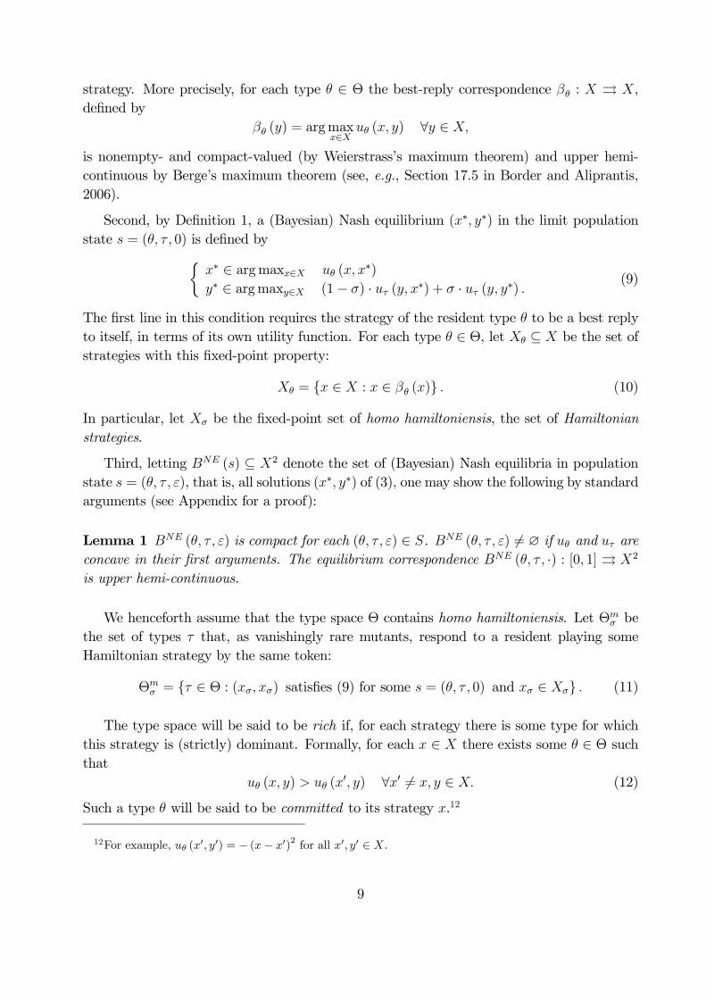
strategy. More precisely, for each type ∈ Θ the best-reply correspondence : ⇒ ,

defined by

() = argmax∈

( ) ∀ ∈

is nonempty- and compact-valued (by Weierstrass’s maximum theorem) and upper hemi-

continuous by Berge’s maximum theorem (see, e.g., Section 17.5 in Border and Aliprantis,

2006).

Second, by Definition 1, a (Bayesian) Nash equilibrium (∗ ∗) in the limit populationstate = ( 0) is defined by½

∗ ∈ argmax∈ ( ∗)

∗ ∈ argmax∈ (1− ) · ( ∗) + · ( ∗) (9)

The first line in this condition requires the strategy of the resident type to be a best reply

to itself, in terms of its own utility function. For each type ∈ Θ, let ⊆ be the set of

strategies with this fixed-point property:

= { ∈ : ∈ ()} (10)

In particular, let be the fixed-point set of homo hamiltoniensis, the set of Hamiltonian

strategies.

Third, letting () ⊆ 2 denote the set of (Bayesian) Nash equilibria in population

state = ( ), that is, all solutions (∗ ∗) of (3), one may show the following by standardarguments (see Appendix for a proof):

Lemma 1 ( ) is compact for each ( ) ∈ . ( ) 6= ∅ if and areconcave in their first arguments. The equilibrium correspondence ( ·) : [0 1] ⇒ 2

is upper hemi-continuous.

We henceforth assume that the type space Θ contains homo hamiltoniensis. Let Θ be

the set of types that, as vanishingly rare mutants, respond to a resident playing some

Hamiltonian strategy by the same token:

Θ = { ∈ Θ : ( ) satisfies (9) for some = ( 0) and ∈ } (11)

The type space will be said to be rich if, for each strategy there is some type for which

this strategy is (strictly) dominant. Formally, for each ∈ there exists some ∈ Θ such

that

( ) (0 ) ∀0 6= ∈ (12)

Such a type will be said to be committed to its strategy .12

12For example, (0 0) = − (− 0)2 for all 0 0 ∈ .

9

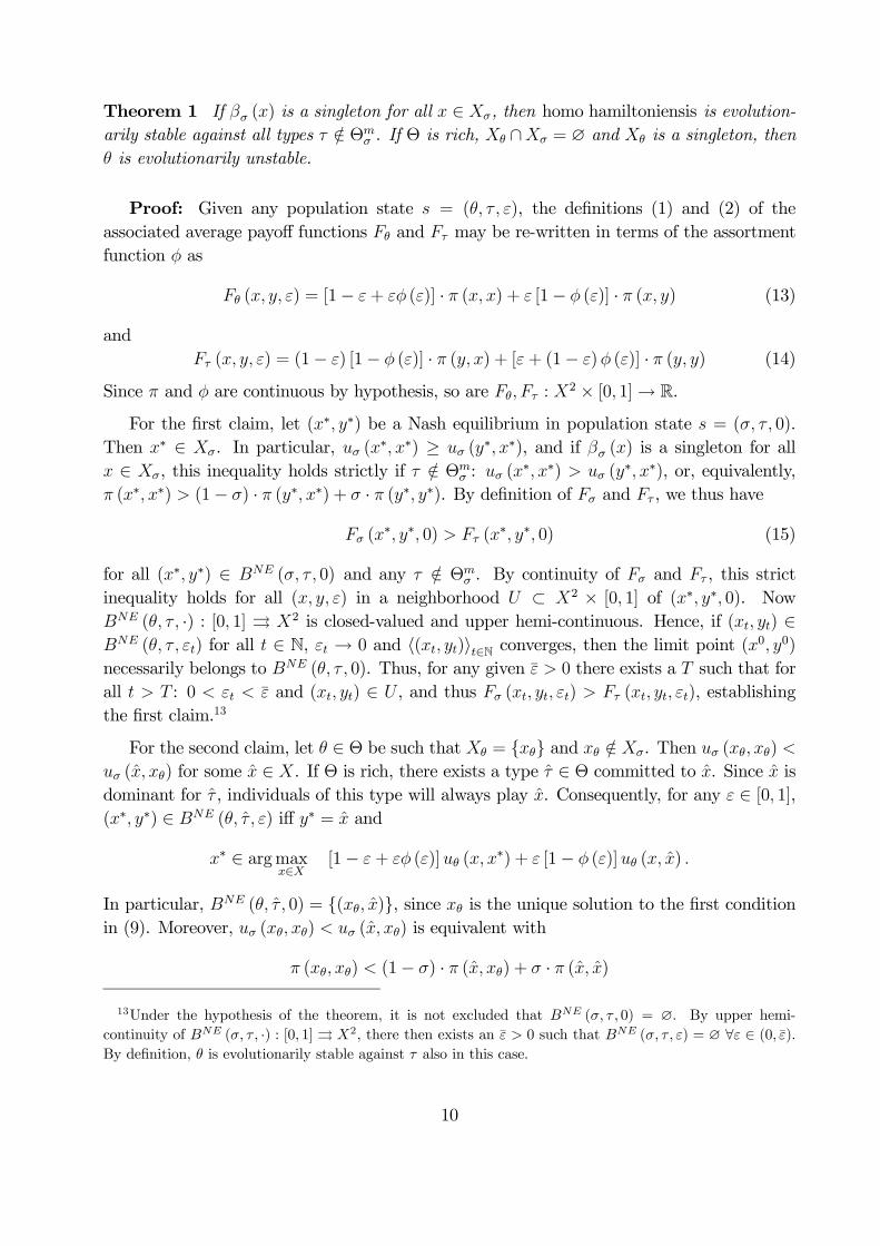
Theorem 1 If () is a singleton for all ∈ , then homo hamiltoniensis is evolution-

arily stable against all types ∈ Θ . If Θ is rich, ∩ = ∅ and is a singleton, then

is evolutionarily unstable.

Proof: Given any population state = ( ), the definitions (1) and (2) of the

associated average payoff functions and may be re-written in terms of the assortment

function as

( ) = [1− + ()] · ( ) + [1− ()] · ( ) (13)

and

( ) = (1− ) [1− ()] · ( ) + [+ (1− ) ()] · ( ) (14)

Since and are continuous by hypothesis, so are : 2 × [0 1]→ R.

For the first claim, let (∗ ∗) be a Nash equilibrium in population state = ( 0).

Then ∗ ∈ . In particular, (∗ ∗) ≥ (

∗ ∗), and if () is a singleton for all ∈ , this inequality holds strictly if ∈ Θ

: (∗ ∗) (

∗ ∗), or, equivalently, (∗ ∗) (1− ) · (∗ ∗) + · (∗ ∗). By definition of and , we thus have

(∗ ∗ 0) (

∗ ∗ 0) (15)

for all (∗ ∗) ∈ ( 0) and any ∈ Θ . By continuity of and , this strict

inequality holds for all ( ) in a neighborhood ⊂ 2 × [0 1] of (∗ ∗ 0). Now

( ·) : [0 1] ⇒ 2 is closed-valued and upper hemi-continuous. Hence, if ( ) ∈ ( ) for all ∈ N, → 0 and h( )i∈N converges, then the limit point (0 0)necessarily belongs to ( 0). Thus, for any given 0 there exists a such that for

all : 0 and ( ) ∈ , and thus ( ) ( ), establishing

the first claim.13

For the second claim, let ∈ Θ be such that = {} and ∈ . Then ( )

( ) for some ∈ . If Θ is rich, there exists a type ∈ Θ committed to . Since is

dominant for , individuals of this type will always play . Consequently, for any ∈ [0 1],(∗ ∗) ∈ ( ) iff ∗ = and

∗ ∈ argmax∈

[1− + ()] ( ∗) + [1− ()] ( )

In particular, ( 0) = {( )}, since is the unique solution to the first conditionin (9). Moreover, ( ) ( ) is equivalent with

( ) (1− ) · ( ) + · ( )

13Under the hypothesis of the theorem, it is not excluded that ( 0) = ∅. By upper hemi-

continuity of ( ·) : [0 1] ⇒ 2, there then exists an 0 such that ( ) = ∅ ∀ ∈ (0 ).By definition, is evolutionarily stable against also in this case.

10

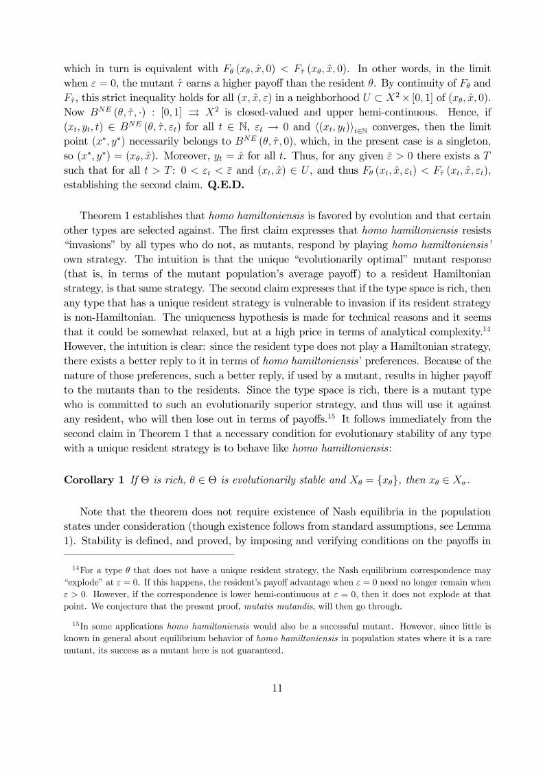
which in turn is equivalent with ( 0) ( 0). In other words, in the limit

when = 0, the mutant earns a higher payoff than the resident . By continuity of and

, this strict inequality holds for all ( ) in a neighborhood ⊂ 2× [0 1] of ( 0).Now ( ·) : [0 1] ⇒ 2 is closed-valued and upper hemi-continuous. Hence, if

( ) ∈ ( ) for all ∈ N, → 0 and h( )i∈N converges, then the limitpoint (∗ ∗) necessarily belongs to ( 0), which, in the present case is a singleton,

so (∗ ∗) = ( ). Moreover, = for all . Thus, for any given 0 there exists a

such that for all : 0 and ( ) ∈ , and thus ( ) ( ),

establishing the second claim. Q.E.D.

Theorem 1 establishes that homo hamiltoniensis is favored by evolution and that certain

other types are selected against. The first claim expresses that homo hamiltoniensis resists

“invasions” by all types who do not, as mutants, respond by playing homo hamiltoniensis’

own strategy. The intuition is that the unique “evolutionarily optimal” mutant response

(that is, in terms of the mutant population’s average payoff) to a resident Hamiltonian

strategy, is that same strategy. The second claim expresses that if the type space is rich, then

any type that has a unique resident strategy is vulnerable to invasion if its resident strategy

is non-Hamiltonian. The uniqueness hypothesis is made for technical reasons and it seems

that it could be somewhat relaxed, but at a high price in terms of analytical complexity.14

However, the intuition is clear: since the resident type does not play a Hamiltonian strategy,

there exists a better reply to it in terms of homo hamiltoniensis’ preferences. Because of the

nature of those preferences, such a better reply, if used by a mutant, results in higher payoff

to the mutants than to the residents. Since the type space is rich, there is a mutant type

who is committed to such an evolutionarily superior strategy, and thus will use it against

any resident, who will then lose out in terms of payoffs.15 It follows immediately from the

second claim in Theorem 1 that a necessary condition for evolutionary stability of any type

with a unique resident strategy is to behave like homo hamiltoniensis:

Corollary 1 If Θ is rich, ∈ Θ is evolutionarily stable and = {}, then ∈ .

Note that the theorem does not require existence of Nash equilibria in the population

states under consideration (though existence follows from standard assumptions, see Lemma

1). Stability is defined, and proved, by imposing and verifying conditions on the payoffs in

14For a type that does not have a unique resident strategy, the Nash equilibrium correspondence may

“explode” at = 0. If this happens, the resident’s payoff advantage when = 0 need no longer remain when

0. However, if the correspondence is lower hemi-continuous at = 0, then it does not explode at that

point. We conjecture that the present proof, mutatis mutandis, will then go through.

15In some applications homo hamiltoniensis would also be a successful mutant. However, since little is

known in general about equilibrium behavior of homo hamiltoniensis in population states where it is a rare

mutant, its success as a mutant here is not guaranteed.

11

those Nash equilibria that do exist. Hence, if for some types ∈ Θ there would exist

no Nash equilibrium in any state ( ) with small, then will be deemed evolutionarily

stable against according to our definition by “walk over.” If this turns out to be a real issue

in some application, one can of course restrict the type space to concave utility functions,

since this guarantees the existence of Nash equilibria in all population states.

Example 1 As an illustration of Theorem 1, consider a canonical public-goods situation.

Let ( ) = (+ )− () for : [0]→ R twice differentiable with 0 0 00 0and 00 0 and 0 such that 0 (0) 0 (0) and 0 (2) 20 (2). Here (+ ) is

the public benefit and () the private cost from one’s own contribution when the other

individual contributes . Played by two homo moralis with degree of morality ∈ [0 1],this interaction defines a game with a unique Nash equilibrium, and this is symmetric. The

equilibrium contribution, , is the unique solution in (0) to the first-order condition

0 () = (1 + )0 (2). Hence, = {}. We note that homo moralis’ contributionincreases from that of the selfish homo oeconomicus when = 0 to that of a benevolent

social planner when = 1. Moreover, it is easily verified that () is a singleton for all

∈ [0]. Theorem 1 establishes that homo hamiltoniensis, that is homo moralis with degreeof morality = , is evolutionarily stable against all types that, as vanishingly rare mutants,

would contribute 6= . Moreover, if Θ is rich, and ∈ Θ is any type that has a unique

resident strategy and this differs from , then is evolutionarily unstable.

3.1 Homo oeconomicus

Theorem 1 may be used to pin down evolutionary stability properties of homo oeconomicus.

The most general formulation is as follows:

Corollary 2 If = 0 and 0 () is a singleton for all ∈ 0, then homo oeconomicus

is evolutionarily stable against all types ∈ Θ0 . If 0 and Θ is rich, then homo

oeconomicus is evolutionarily unstable if it has a unique resident strategy and this does not

belong to .

The first part of this result says that a sufficient condition for homo oeconomicus to be

evolutionarily stable against mutants who play other strategies than homo oeconomicus is

that the index of assortativity be zero. This result is in line with Ok and Vega-Redondo

(2001) and Dekel et al. (2007), who both analyze the evolution of preferences under incom-

plete information and uniform random matching.

The second part says that if the index of assortativity is positive, then homo oeconomicus

is evolutionarily unstable when it has a unique resident strategy and this is not Hamiltonian.

To further clarify the implications of this result, we distinguish two classes of interactions,

according to whether or not an individual’s payoff depends on the other individual’s strategy.

12

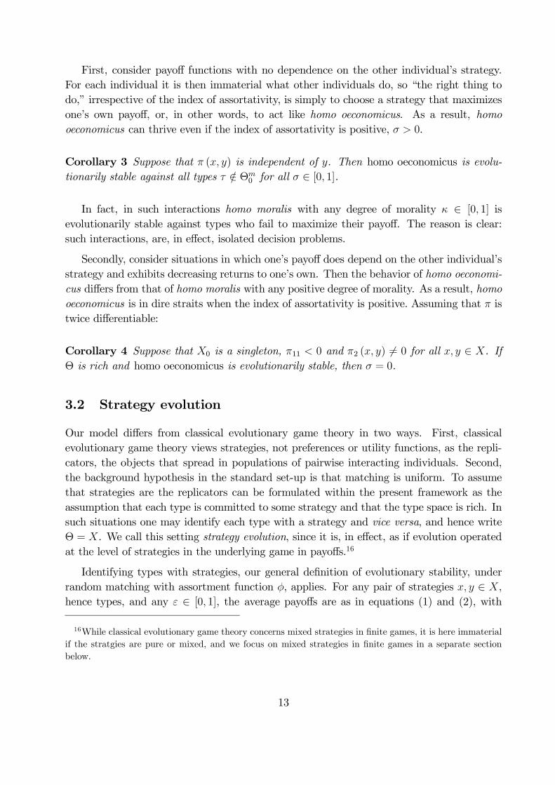
First, consider payoff functions with no dependence on the other individual’s strategy.

For each individual it is then immaterial what other individuals do, so “the right thing to

do,” irrespective of the index of assortativity, is simply to choose a strategy that maximizes

one’s own payoff, or, in other words, to act like homo oeconomicus. As a result, homo

oeconomicus can thrive even if the index of assortativity is positive, 0.

Corollary 3 Suppose that ( ) is independent of . Then homo oeconomicus is evolu-

tionarily stable against all types ∈ Θ0 for all ∈ [0 1].

In fact, in such interactions homo moralis with any degree of morality ∈ [0 1] is

evolutionarily stable against types who fail to maximize their payoff. The reason is clear:

such interactions, are, in effect, isolated decision problems.

Secondly, consider situations in which one’s payoff does depend on the other individual’s

strategy and exhibits decreasing returns to one’s own. Then the behavior of homo oeconomi-

cus differs from that of homo moralis with any positive degree of morality. As a result, homo

oeconomicus is in dire straits when the index of assortativity is positive. Assuming that is

twice differentiable:

Corollary 4 Suppose that 0 is a singleton, 11 0 and 2 ( ) 6= 0 for all ∈ . If

Θ is rich and homo oeconomicus is evolutionarily stable, then = 0.

3.2 Strategy evolution

Our model differs from classical evolutionary game theory in two ways. First, classical

evolutionary game theory views strategies, not preferences or utility functions, as the repli-

cators, the objects that spread in populations of pairwise interacting individuals. Second,

the background hypothesis in the standard set-up is that matching is uniform. To assume

that strategies are the replicators can be formulated within the present framework as the

assumption that each type is committed to some strategy and that the type space is rich. In

such situations one may identify each type with a strategy and vice versa, and hence write

Θ = . We call this setting strategy evolution, since it is, in effect, as if evolution operated

at the level of strategies in the underlying game in payoffs.16

Identifying types with strategies, our general definition of evolutionary stability, under

random matching with assortment function , applies. For any pair of strategies ∈ ,

hence types, and any ∈ [0 1], the average payoffs are as in equations (1) and (2), with

16While classical evolutionary game theory concerns mixed strategies in finite games, it is here immaterial

if the stratgies are pure or mixed, and we focus on mixed strategies in finite games in a separate section

below.

13

being the type committed to and the type committed to . The difference function

() ≡ ( )− ( ) (with committed to and to ) is a generalization of

what in standard evolutionary game theory is called the score function of strategy against

strategy .17 Applied to the present setting of strategy evolution, the stability definition in

Section 2 boils down to:

Definition 5 Let Θ = (strategy evolution) and consider random matching with assort-

ment function . A strategy ∈ is evolutionarily stable against a strategy ∈ if

there exists an ∈ (0 1) such that () 0 for all ∈ (0 ). A strategy is evolution-arily stable if it is evolutionarily stable against all 6= in .

We immediately obtain from Theorem 1:18

Corollary 5 Let Θ = (strategy evolution). Every strategy ∈ for which () is

a singleton is evolutionarily stable. Every strategy ∈ is evolutionarily unstable.

Proof: For the first claim, let ∈ and 6= . In a population state = ( ),

the expected payoff to is

() = [1− + ()] · ( ) + [1− ()] · ( )

and that to is

() = [+ (1− ) ()] · ( ) + (1− ) [1− ()] · ( )

(see equations (13) and (14)). It follows that : [0 1] → R are continuous. Hence, asufficient condition for to be evolutionarily stable against is that (0) (0), or,

equivalently,

( ) (1− ) · ( ) + · ( ) or ( ) ( ). If () is a singleton, the last inequality holds for all 6= .

This establishes the first claim.

For the second claim, let ∈ . Then ( ) ( ) for some ∈ . Equiva-

lently,

( ) (1− ) · ( ) + · ( )

17In the standard theory (Bomze and Pötscher, 1989, and Weibull, 1995), ≡ 0, so that () = (1− ) ( ) + ( )− ( )− (1− ) ( )

18Note that here homo hamiltoniensis is not included in the type space. Homo hamiltoniensis is instead

represented by one type for each Hamiltonian strategy. The theorem nonetheless refers to the best-reply

correpondence . This is because we allow for a very general class of assortment functions . In Proposition

1 we dispense with the assumption of a singleton-valued because we there impose more structure on .

14

or, equivalently, (0) (0). By continuity of : [0 1] → , this implies that is

evolutionarily unstable. Q.E.D.

In other words, every Hamiltonian strategy which is its own unique best reply is evolu-

tionarily stable, and all non-Hamiltonian strategies are evolutionarily unstable. In the special

case of uniform random matching, = 0, the Hamiltonian strategies are simply those that

are best replies to themselves in terms of payoffs. In the opposite extreme case, = 1, the

Hamiltonian strategies are those that, when used by both players, result in Pareto efficiency

in terms of payoffs.

Remark 3 For payoff functions such that homo hamiltoniensis has a unique best reply to all

Hamiltonian strategies, Theorem 1 and Corollary 5 establish that preference evolution under

incomplete information induces the same behaviors as strategy evolution.

For certain payoff functions , the Hamiltonian best-reply correspondence is not singleton-

valued. The following characterization is a generalization of Maynard Smith’s and Price’s

(1973) original definition and does not require singleton-valuedness. The hypothesis is in-

stead that the degree of assortment is independent of the population share , a property that

holds in certain kinship relations, see Section 7.

Proposition 1 Let Θ = (strategy evolution) and assume that the assortment function is

a constant, () ≡ . A strategy ∈ is evolutionarily stable if and only if

( ) ≥ ( ) + · [ ( )− ( )] ∀ ∈ (16)

and

( ) = ( ) + · [ ( )− ( )] (17)

⇒ ( ) ( ) + · [ ( )− ( )]

Proof: Suppose that () = ∈ [0 1] for all ∈ (0 1). Then

() = (1− + ) · ( ) + (1− ) · ( )− [+ (1− )] · ( )− (1− ) (1− ) · ( )

which defines (for given and 6= ) as an affine function of . A strategy is

evolutionarily stable iff () 0 on some non-empty interval (0 ). A necessary condition

for this is clearly (0) ≥ 0, or, equivalently, (16). If the latter holds with equality, then itis necessary that the slope of be positive, or, equivalently, (17). Conversely, if (16) and

(17) both hold, then (0) ≥ 0, and, in case (0) = 0, the slope of is positive, so is evolutionarily stable. Q.E.D.

15

The necessary condition (16) can be written as ∈ , that is, the strategy must be

Hamiltonian. Further, condition (17) may be written

( ) = ( ) + · [ ( )− ( )]

⇒ ( ) + ( )− ( )− ( ) 0

a formulation that agrees with Hines’ and Maynard Smith’s (1979) analysis of ESS for games

played by relatives. See also Grafen (1979, 2006).

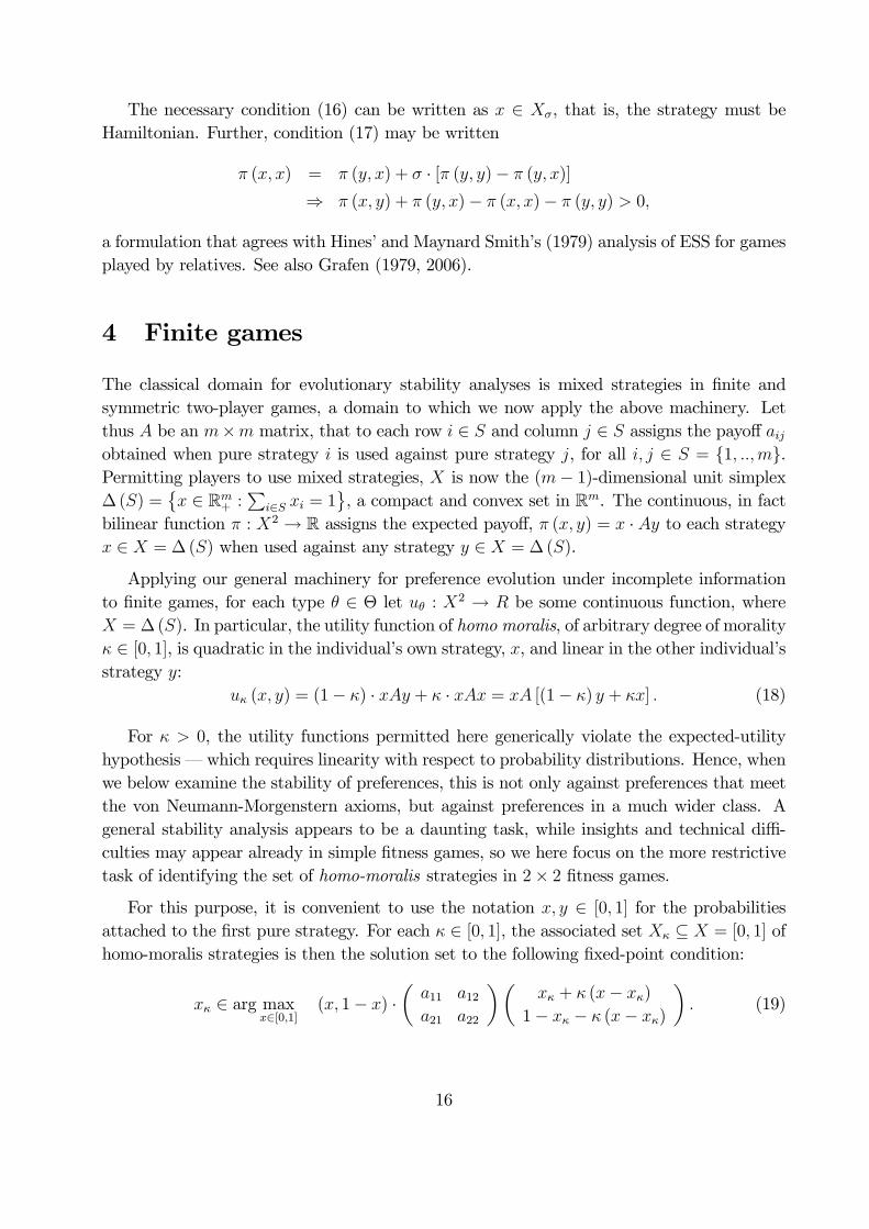
4 Finite games

The classical domain for evolutionary stability analyses is mixed strategies in finite and

symmetric two-player games, a domain to which we now apply the above machinery. Let

thus be an × matrix, that to each row ∈ and column ∈ assigns the payoff

obtained when pure strategy is used against pure strategy , for all ∈ = {1 }.Permitting players to use mixed strategies, is now the (− 1)-dimensional unit simplex∆ () =

© ∈ R

+ :P

∈ = 1ª, a compact and convex set in R. The continuous, in fact

bilinear function : 2 → R assigns the expected payoff, ( ) = · to each strategy ∈ = ∆ () when used against any strategy ∈ = ∆ ().

Applying our general machinery for preference evolution under incomplete information

to finite games, for each type ∈ Θ let : 2 → be some continuous function, where

= ∆ (). In particular, the utility function of homo moralis, of arbitrary degree of morality

∈ [0 1], is quadratic in the individual’s own strategy, , and linear in the other individual’sstrategy :

( ) = (1− ) · + · = [(1− ) + ] (18)

For 0, the utility functions permitted here generically violate the expected-utility

hypothesis – which requires linearity with respect to probability distributions. Hence, when

we below examine the stability of preferences, this is not only against preferences that meet

the von Neumann-Morgenstern axioms, but against preferences in a much wider class. A

general stability analysis appears to be a daunting task, while insights and technical diffi-

culties may appear already in simple fitness games, so we here focus on the more restrictive

task of identifying the set of homo-moralis strategies in 2× 2 fitness games.For this purpose, it is convenient to use the notation ∈ [0 1] for the probabilities

attached to the first pure strategy. For each ∈ [0 1], the associated set ⊆ = [0 1] of

homo-moralis strategies is then the solution set to the following fixed-point condition:

∈ arg max∈[01]

( 1− ) ·µ

11 12

21 22

¶µ + (− )

1− − (− )

¶ (19)

16

Depending on whether the sum of the diagonal elements of exceeds, equals or falls short

of the sum of its off-diagonal elements, the utility of homo moralis is either strictly convex,

linear, or strictly concave in his/her own strategy, so that the following result obtains:

Proposition 2 Let

() = min

½1

12 + 21 − (1 + ) 22

(1 + ) (12 + 21 − 11 − 22)

¾ (20)

(a) If 0 and 11 + 22 12 + 21, then ⊆ {0 1}.(b) If = 0 and/or 11 + 22 = 12 + 21, then

=

⎧⎨⎩{0} if 12 + 21 (1 + ) 22

[0 1] if 12 + 21 = (1 + ) 22

{1} if 12 + 21 (1 + ) 22

(c) If 0 and 11 + 22 12 + 21, then

=

½ {0} if 12 + 21 ≤ (1 + ) 22

{ ()} if 12 + 21 (1 + ) 22

Proof : The maximand in (19) can be written as

(11 + 22 − 12 − 21) · 2 + (1− ) (11 + 22 − 12 − 21) · + [12 + 21 − (1 + ) 22] · + (1− ) · (21 − 22) + 22

For (11 + 22 − 12 − 21) 0, this is a strictly convex function of , and hence the

maximum is achieved on the boundary of = [0 1]. This proves claim (a).

For (11 + 22 − 12 − 21) = 0, the maximand is affine in , with slope 12 + 21 −(1 + ) 22. This proves (b).

For (11 + 22 − 12 − 21) 0, the maximand is a strictly concave function of , with

unique global minimum (in R) at

=12 + 21 − (1 + ) 22

(1 + ) (12 + 21 − 11 − 22)

Hence, = {0} if ≤ 0, = {} if ∈ [0 1], and = {1} if 1, which proves (c).

Q.E.D.

Remark 4 It is seen in (20) that the set of homo-moralis strategies is invariant under

positive affine transformations of payoffs. More generally, if is any × payoff-matrix

and ∗ = +, where is any positive scalar, any positive or negative scalar, and is

the ×-matrix with all entries equal to 1, then the best-reply correspondence associated

with in (18) is unaffected if is replaced by ∗.

17

As an illustration, we identify the set of homo-moralis strategies, for each ∈ [0 1],in a one-shot prisoners’ dilemma with payoff matrix

=

µ

¶(21)

where we assume that − − 0. Case (c) of Proposition 2 then applies for all

0, and an interior solution, () ∈ (0 1), obtains for intermediate values of . Moreprecisely, = {0} for all ≤ ( − ) ( − ), = {1} for all ≥ ( −) (− ),

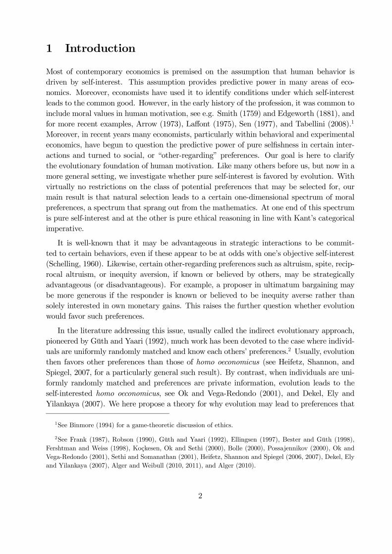
and = { ()} for all between these two bounds. See Figure 1 below, which shows howco-operation increases as the degree of morality increases.

0.0 0.5 1.00.0

0.5

1.0

kappa

x-kappa

Figure 1: The (singleton) set of homo-moralis strategies for ( ) = (7 5 3 2).

5 Matching processes

Most of the literature on preference evolution has focused on the case of when all matchings

are equally likely.19 Under such uniform randommatching, Pr [| ] = Pr [| ] = 1−, andhence there is no assortativity: () = 0 for all ∈ (0 1). Arguably, positive assortativityarises naturally in many, if not most, human interactions, due to socioeconomic population

structure, limited social or geographical mobility, habitat preferences, local customs and

cultures etc., see Eshel and Cavalli-Sforza (1982) and Bergstrom (1995, 2003). In this section

we explore a variety of such possibilities, and identify the associated index of assortativity,

.

Broadly speaking, whether preferences are transmitted genetically or culturally, assorta-

tivity is positive as soon as there is a positive probability that both parties in an interaction

have inherited their preferences (or moral values) from a common “ancestor” (genetic or

cultural).

19Exceptions are Alger and Weibull (2010, 2011), and Alger (2010), who allow for assortativeness when

analyzing the evolution of preferences under complete information. Hines and Maynard Smith (1979), Grafen

(1979), Bergstrom (1995, 2003) and Day and Taylor (1998) allow for assortativeness in models of strategy

evolution. See Gardner and West (2004) for an account of how negative assortativity may arise.

18

5.1 Interactions between kin

While the following arguments can readily be adapted to interactions between other kin (see

Alger and Weibull, 2011), here we study pairwise interactions between siblings, for which

preferences are not gender specific. Consider a population of grown-ups where a proportion

1 − have preferences of type ∈ Θ and the residual proportion has preferences of type

∈ Θ, the same proportion among men as among women, and suppose that couples are

formed randomly with respect to their preference types – “random mating”. We here show

how the index of assortativity between siblings then depends on whether a child inherits

his/her type from the parents or from others in society, and if the former case, whether the

siblings have the same parents.

5.1.1 Vertical transmission

Assume that each child is equally likely to inherit each parent’s preference type (and these

random draws are statistically independent). The inheritance mechanism could be genetic

or cultural.20 Suppose, first, that siblings have the same parents.

Proposition 3 Under random mating and monogamy, () = 12 for all ∈ (0 1).

Proof: Consider a population where a proportion ∈ (0 1) of the adult populationcarries type , and a proportion 1− carries type . A -child necessarily has at least one

-parent. With probability 1−, the other parent also has type , in which case both siblingsmust have type . If the other parent has type , which happens with probability , the

other sibling has type with probability 12 and type with probability 12. Hence, the

probability that a -child’s sibling also is a -child is Pr [| ] = 1−2. Similarly, a -childhas at least one -parent. With probability 1− the other parent has type , in which case

the probability that the sibling has type is 12. Hence, the probability that a -child’s

sibling has type is Pr [| ] = (1− ) 2. We obtain () = Pr [| ]− Pr [| ] = 12.Q.E.D.

Note that = 12 is the coefficient of relatedness between siblings (Wright, 1922).

Second, suppose, still, that there is random matching among parents, but that siblings

always have different fathers.21

20In biological terms, we here focus on sexual reproduction in a haploid species. Thus, each child has

two genetic parents, and each parent carries one set of chromosomes, and this determines heredity. Humans

are a diploid species, with two sets of chromosomes, which complicates matters because of the distinction

between recessive and dominant genes. For calculations of assortativeness in diploid species, see Bergstrom

(1995, 2003). See further Michod and Hamilton (1980).

21The same result holds under polygyny, that is, when (half-)siblings always have the same father but

different mothers.

19

Proposition 4 Under random mating and polyandry, () = 14 for all ∈ (0 1).

(A proof is given in a working paper available on our personal web sites.) As in the case

with full siblings, here = 14 is the coefficient of relatedness between half-siblings (Wright,

1922).

These results can be combined to calculate the index of assortativity between siblings

in a population where some parents remain monogamous while others divorce after the first

child and get a new child with their new partner.

Proposition 5 Suppose that a fraction ∈ [0 1] of couples divorce. Then () = 12 −4 for all ∈ (0 1).

Proof: For children whose parents did not divorce, () = 12, see Proposition 3. For

children whose parents did divorce, () = 14, see Proposition 4. On average, then, in the

child population: () = (1− ) 2 + 4 = 12− 4. Q.E.D.

5.1.2 Oblique transmission

The above examples apply to both genetic and cultural transmission from parents to children.

But “cultural parents” (or role models) other than the parents can also be encompassed in

the framework, along the lines suggested by Bisin and Verdier (2001). This may happen

when social values spread through institutions other than the family, such as schools, media,

religious institutions etc.

Proposition 6 Assume monogamy, but suppose now that each child inherits a parent’s pref-

erences with probability ∈ [0 1], that otherwise the child takes on the preferences of a uni-formly randomly drawn grown-up, from the population at large, and that the siblings’ choices

of role model are statistically independent. Then = 22.

Proof: Let ∈ (0 1). For a child born into a family where both children inherited theirpreferences from their parents, () = 12, as in Proposition 3. This is the case for the

fraction 2 of all sibling pairs. For a child born into a family where at least one child’s type

was drawn from a random grown-up in the population, () ≈ . Q.E.D.

5.2 Interactions among non-kin

For a variety of interactions among non-kin, education, population structure, social struc-

ture, culture, ethnicity, geography, networks, customs and habits, may all lead to various

deviations from uniform randomness in the pairwise matchings.

20

5.2.1 Education

Assortativity may arise in business partnerships. To see this, consider a large population

engaged in pairwise business partnerships, represented by a symmetric fitness game hi.Suppose that each individual acquires her preferences concerning business strategies in school

and enters a new two-person business partnership upon finishing school. Now and then, a

school changes the business values they teach.

Proposition 7 Let ∈ [0 1] be the probability that a newly minted graduate forms a busi-ness partnership with a former schoolmate, and suppose that otherwise the graduate forms a

partnership with a graduate uniformly randomly drawn from the whole pool of newly minted

graduates in society at large. Then = .

Proof: Consider a large collection of schools, where the proportion 1− teach a businessvalue system ∈ Θ and a proportion teaches a business value system . Let → 0. For

graduates pairing up with a former schoolmate, = 1. For all other graduates, = 0. Since

there is a fraction of graduates who pair up with a schoolmate, on average, then, in the

population of newly minted graduates, = . Q.E.D.

5.2.2 Migration

In pre-historic societies, assortativity may have come about as a result of migration patterns.

Consider a society in which individuals grow up in small communities, where each community

has a hunting team consisting of two men from the community, where each community

teaches some values system for how to act in a hunting team to their youngsters, and that

some young men migrate from one community to another after their training but before they

become members of a hunting team (for example because of marriage).

Proposition 8 Suppose that a fraction ∈ [0 1] of the young men migrate from their nativecommunity to a uniformly randomly drawn community in society at large, while the others

remain in their native community. Then = 1− .

Proof: Consider a large collection of communities, where the proportion 1 − teaches

hunting values and the proportion teaches hunting values . For men who remained

in their native community, = 1 − , while for men who moved, = 0. Since there is a

fraction 1− of young men who remain in their native community, on average, then, in the

population of young men, = (1− ). Q.E.D.

In traditional societies, migration is often linked to marriage, and typically tradition

dictates whether the bride or bridegroommigrates. Thus, our model suggests that differences

in marriage customs may have affected the evolution of preferences within each gender.

21

6 Discussion

6.1 Related literature

The idea that moral values may have been formed by evolutionary forces is evidently not

new, and there is a substantial literature on this theme. The idea can be traced back to at

least Darwin (1871). More recent treatments include, to mention a few, Alexander (1987),

Nichols (2004) and de Waal (2006). The latter claims that there is evidence that moral codes

also exist in other primates. In this literature, mathematical analyses are rare, however.

An exception is the work by Bergstrom (1995, 2009). Bergstrom (1995) studies strategy

evolution in sibling interactions, where strategies are genetically transmitted from parents to

children. He finds that evolution favors strategies that are as though individuals had Kantian

preferences under asexual reproduction, and “semi-Kantian preferences” under sexual diploid

reproduction with recessive genes. This is exactly in line with our findings, since = 1 under

asexual reproduction and = 12 under sexual diploid reproduction with recessive genes.

Bergstrom (2009) extends this reasoning to arbitrary degrees of relatedness, and also provides

a thought-provoking discussion and interpretation of various moral maxims.22

6.2 Morality vs. altruism

There is a large body of theoretical research on the evolution of altruism (e.g., Becker,

1976, Hirshleifer, 1977, Bester and Güth, 1998, Bolle, 2000, Possajennikov, 2000, Alger

and Weibull, 2010, 2011, and Alger, 2010). Altruism towards another individual is often

represented in parametric form by letting the utility function of the altruist be the sum of

two terms, where the first term is his or her own payoff and the other term is the other

individual’s payoff multiplied by a factor ∈ [0 1]. In the present context,

( ) = ( ) + ( ) (22)

for some degree of altruism ∈ [0 1]. By contrast, our homo moralis has preferences of theform

( ) = (1− ) ( ) + ( ) (23)

for some degree of of morality ∈ [0 1]. Hence, while an altruist cares about the other’spayoff, homo moralis cares about what is the “right thing to do,” irrespective of what the

other party actually does or is expected to do. We first show that while in some situations,

morality and altruism lead to the same behavior, in others the contrast is stark. Second, we

discuss a situation where the behavior of homo moralis can be viewed as less “moral” than

that of an altruist, or even than that of homo oeconomicus.

22Unlike us, however, Bergstrom (1995, 2009) bases his analysis on pure strategies in finite games, rather

than on mixed strategies, as we here do.

22

The necessary first-order condition for an altruist at an interior symmetric equilibrium,

[1 ( ) + 2 ( )]|= = 0

is identical with that for a homo moralis,

[(1− )1 ( ) + 1 ( ) + 2 ( )]|= = 0

if = . Nonetheless, there is an important qualitative difference between homo moralis and

altruists, namely, that their utility functions are in general not monotonic transformations

of each other. This is seen in equations (22) and (23): for non-trivial payoff functions

and strategy sets , and for any 6= 0, there exists no function : R → R such that [ ( )] = ( ) for all ∈ . This is seen most clearly in the case of finite games.

Then is linear in while is quadratic in :½ ( ) = · + · ( ) = (1− ) · + ·

Consequently, the best-reply correspondence of an altruist in general differs qualitatively

from the best-reply correspondence of homo moralis, even when = . Indeed, the

equilibria among altruists may differ from the equilibria among homo moralis also when

= .

We further illustrate the tension between moralists and altruists, now in a finite game,

an example suggested to us by Ariel Rubinstein. Let

=

µ 2

1 0

¶for some ∈ (0 1). Consider a homo kantiensis ( = 1), the “most moral” among homo

moralis. Such a creature will always play

=1 =3

6− 2

Suppose now that such an individual visits a country where everyone always plays the

first pure strategy, thus earning payoff in each encounter with each other. When homo

kantiensis interacts with a citizen in that society, the matched native earns more than when

interacting with other natives. However, if the visitor instead were a homo oeconomicus

( = 0), then this new visitor would play the second pure strategy. Consequently, the

other individual in the match would earn more than in a meeting with homo kantiensis. In

fact, this lucky citizen would earn the maximal payoff in this game. Hence, citizens in this

country would be even more delighted to interact with homo oeconomicus than with homo

kantiensis. Should then homo oeconomicus be deemed “less moral” than homo kantiensis in

this situation? What if we would instead replace homo kantiensis by a full-blooded altruist,

23

someone who maximizes the sum of payoffs ( = 1)? Given that all citizens always play

the first pure strategy, the best such an altruist could do would be to play the second pure

strategy, just as homo oeconomicus would.

This example illustrates that homo kantiensis is not necessarily “more moral” in an

absolute sense and in all circumstances, than, say homo oeconomicus or an altruist. However,

homo kantiensis is more moral in the sense of always acting in accordance with a general

principle that is independent of the situation and identity of the actor (moral universalism),

namely to do that which, if done by everybody, maximizes everybody’s payoff.

Remark 5 Suppose that the citizens of the country imagined above would like to achieve

the highest possible payoff but are not even aware of the second pure strategy. Then homo

kantiensis would, by his own example, show them its existence and thus how they can increase

their payoff in encounters amongst themselves. Indeed, an entrepreneurial and benevolent

visitor to the imagined country could go one step further and suggest a simple institution

within which to play this game, namely an initial random role allocation, at each pairwise

match, whereby one individual is assigned player role 1 and the other player role 2, with

equal probability for both allocations. This defines another symmetric two-player game in

which each player has four pure strategies (two for each role). In this “meta-game” 0,homo kantiensis would use any of two strategies 0=1, each of which would maximize thepayoff 0 (0=1

0=1), namely to either always play the first (second) pure strategy in the

original game when in player role 1 (2), or vice versa. In both cases, 0 (0=1 0=1) = 32, a

higher payoff than when homo kantiensis meets himself in the original game: (=1 =1) =

(2− 23)−1 · 32.

6.3 Empirical testing

An interesting empirical research challenge is to find out how well homo moralis can explain

behavior observed in controlled laboratory experiments. Consider, for example, an experi-

ment in which (a) subjects are randomly and anonymously matched in pairs to play some

two-player game in monetary payoffs (or a few different such games), (b) after the first few

rounds of play, under random re-matching, subjects receive some information about aggre-

gate play in these early rounds, and (c) are then invited to play some more rounds (again

with randomly drawn opponents). One could then analyze their behavior in these later

rounds as if they played a (Bayesian) Nash equilibrium under incomplete information, where

each individual is a homo moralis with an individual-specific and presumed fixed degree of

morality (presumably given from that individual’s background, experience and personality).

How much of the observed behavior could be explained this way? If one were to embed the

simple preferences of homo moralis in a more general class of other-regarding preferences,

how much more explanatory power would then be gained? Supposing that the subjects be-

have as they usually do in similar real-world interactions, one could compare estimates of the

24

degrees of morality in different subject pools and see if this seems to map relevant cultural

and socioeconomic differences, in line with homo hamiltoniensis.23

Remark 6 Although in the model above individuals play only one game, the model has

clear implications for the more realistic situation where each individual engages in multiple

interactions. Indeed, the degree of morality that will be selected for will simply correspond to

the index of assortativity in the matching process for the interaction at hand. For instance,

if individuals are recurrently both engaged in some family interaction with a high index of

assortativity and also in some market interaction with a low index of assortativity, then

the above theory says that one and the same individual will tend to exhibit a high degree

of morality in the family interaction and be quite selfish in the market interaction. More

generally, the type of an individual engaged in multiple interactions will be a vector of degrees

of morality, one for each interaction, adapted to the matching processes in question (but

independent of the nature of the interaction).

7 Concluding remarks

Economic analysis is based upon assumptions about human motivation. Presumably, higher

predictive power can be achieved the better the assumptions reflect the actual motivation. In

order to enhance the predictive power of economic models, a deeper understanding of both

proximate and ultimate causes of human motivation is necessary. Our research contributes

to the understanding of ultimate causes, by proposing a theoretical model of the evolution of

preferences.24 We follow a long tradition in the literature by asking whether evolution will

select preferences whereby individuals selfishly maximize their individual fitness payoff.25

So far, the leading theory for why deviations from such preferences may survive evolution

is that, if known or believed by others, such preferences may give its carrier a strategic

commitment advantage in terms of payoff consequences. By contrast, we here show that

23If there is uniform random matching in the lab, then presumably many individuals will gradually, perhaps

quickly for some and slowly (or not at all) for others, change their behavior, during long sessions in the lab,

towards one where they behave more like homo oeconomicus, as it will in our theory if = 0.

24Our theory is, however, silent as to which proximate causes may come into play, and whether it applies

only to humans. Proximate causes may include culture (Gächter and Herrmann, 2009), genes (Cesarini et

al., 2008), and hormones and neural circuitry (Eisenegger et al, 2010, Fehr and Camerer, 2007, Harbaugh

et al., 2007, Moll et al., 2006, Rilling et al., 2002). Pro-social behavior has been observed in other animals,

such as rats (Bartal et al., 2011).

25In a related literature, on cultural evolution, altruistic parents can, at some cost, influence their childrens’

preferences and values; see, e.g., Bisin and Verdier (2001), Hauk and Saez-Martí (2002), Bisin, Topa and

Verdier (2004), and Lindbeck and Nyberg (2006). In our model, evolution is an exogenously given process,

and parents (be they cultural of genetic parents), do not need to be altruistic for non-selfish preferences to

be favored by evolution.

25

deviations from selfish preferences will typically be evolutionarily stable also when preferences

are private information, as long as the matching process that governs interactions involves

some assortativity.26 Our theory thus delivers new, testable predictions, regarding human

motivation.

Although we permit virtually any preferences (as long as they can be represented by

continuous functions), we find that a particular one-dimensional parametric family, the pref-

erences of homo moralis, stands out in the analysis. A homo moralis acts as if he or she

had a sense of morality: she maximizes a weighted sum of own payoff, given her expecta-

tion of the other’s action, and the payoff that she would obtain if both individuals were to

take the same action. A certain member of this family, homo hamiltoniensis, is particularly

viable from an evolutionary perspective. The weight that homo hamiltoniensis attaches to

the second goal is the index of assortativity in the matching process. The viability of homo

hamiltoniensis stems from the fact that the best a mutant can do, in order to “invade” such

a resident population, is to choose the same strategy. Moreover, any resident type that does

not play a Hamiltonian strategy is vulnerable to invasion by mutants.

These results have important implications regarding homo oeconomicus. We show that

homo oeconomicus, who seeks to maximize his own payoff, does well in situations where

there is no assortativity in the matching process and where each individual’s payoff does not

depend on others’ behavior. By contrast, natural selection wipes out homo oeconomicus in

all other situations.27

As is common in the literature, in our model evolutionary success is determined by

behavior in a symmetric interaction. As illustrated by our analyses of the dictator and

ultimatum-bargaining games, the symmetry assumption does not need to apply in a literal

sense, however. The model applies to interactions where there is some asymmetry between

the individuals’ situations (say, helping interactions where one individual happens to be

rich and the other poor), as long as from an ex ante perspective it is not known which

individual will be in which situation. In such cases, evolution selects preferences that favors

the individual, behind the veil of ignorance regarding which situation the individual will

eventually end up in.

While the predictive power of preferences à la homo moralis remains to be analyzed

carefully, we argue that at first glance the behavior of homo moralis seems to be broadly

compatible with experimental evidence. What’s more, homo moralis may explain why many

26This paper complements our work in Alger and Weibull (2010, 2011), and Alger (2010), where we

studied evolutionary stability of preferences under assortative matching and complete information. In that

setting, other factors in the environment (in particular the structure of the payoffs in the interactions driving

evolution) may also affect the evolution of preferences.

27It is important to point out that maximizing own fitness payoff involves acting in an other-regarding

manner if breeding is cooperative or reproduction involves mate competition. For analysis of this, see Weibull

and Salomonsson (2006).

26

subjects justify their behavior in the lab by saying that they wanted to “do the right thing”

(see, e.g., Dawes and Thaler, 1988, Charness and Dufwenberg, 2006). While we leave the-

oretical analyses of the policy implications of such moral preferences for future research,

we note that in our model the degree of morality, that is, the weight attached to the sec-

ond goal, is independent of the interaction at hand. Hence, the degree of morality cannot

be “crowded out” in any direct sense by economic incentives or laws. For instance, if one

were to change an interaction (for example public goods provision) by way of paying people

for “doing the right thing” (say, contributing the socially optimal amount), or by way of

punishing them for doing otherwise, this would change the payoff function, and thus also

the behavior of homo moralis, but in an easily predictable way, since homo moralis cares

neither about other’s opinion of her, nor about other’s actual payoffs. Moreover, our theory

predicts that if one and the same individual is engaged in multiple pairwise interactions of

the sort analyzed here, perhaps with a different index of assortativity associated with each

interaction (say, one interaction taking place within the extended family and another one in

a large anonymous market), then this individual will exhibit different degrees of morality in

these interactions, adapted to the various indices of assortativity.

Some new ground has been covered here, but many deep and important questions about

ultimate causes behind human motivation remain unanswered. For instance, what are the

effects of group size? Can the theory be generalized so as to explain stable preference het-

erogeneity in populations? What happens in truly asymmetric interactions, such as between

parents and children, men and women, or individuals in hierarchies?

27

8 Appendix: Proof of Lemma 1

By hypothesis, and are continuous and is compact. Hence, each right-hand side in

(3) defines a non-empty and compact set, for any given ∈ [0 1], by Weierstrass’s maximumtheorem. For any ( ) ∈ , condition (3) can thus be written in the form (∗ ∗) ∈ (

∗ ∗), where : ⇒ , for = 2 and ∈ [0 1] fixed, is compact-valued, and, byBerge’s maximum theorem, upper hemi-continuous. It follows that has a closed graph,

and hence its set of fixed points, ( ) = {(∗ ∗) ∈ 2 : (∗ ∗) ∈ (∗ ∗)} is

closed (being the intersection of () with the diagonal of 2). This establishes the

first claim.

If and are concave in their first arguments, then so are the maximands in (3).

Hence, is then also convex-valued, and thus has a fixed point by Kakutani’s fixed-point

theorem. This establishes the second claim.

For the third claim, fix and , and write the maximands in (3) as ( ∗ ∗ )and ( ∗ ∗ ). These functions are continuous by assumption. Let ∗ (∗ ∗ ) =max∈ ( ∗ ∗ ) and ∗ (∗ ∗ ) = max∈ ( ∗ ∗ ). These functions are con-tinuous by Berge’s maximum theorem. Note that (∗ ∗) ∈ ( ) iff½

∗ (∗ ∗ )− ( ∗ ∗ ) ≥ 0 ∀ ∈

∗ (∗ ∗ )− ( ∗ ∗ ) ≥ 0 ∀ ∈ (24)

Let hi∈N → ∈ [0 1] and suppose that (∗ ∗ ) ∈ ( ) and (∗

∗ ) → ( ).

By continuity of the functions on the left-hand side in (24),½∗ ( )− ( ) ≥ 0 ∀ ∈

∗ ( )− ( ) ≥ 0 ∀ ∈

and hence ( ) ∈ ( ). This establishes the third claim.

28

ReferencesAlexander, Richard D. 1987. The Biology of Moral Systems. New York: Aldine De

Gruyter.

Alger, Ingela. 2010. “Public Goods Games, Altruism, and Evolution,” Journal of Public

Economic Theory, 12:789-813.

Alger, Ingela, and Jörgen W. Weibull. 2010. “Kinship, Incentives, and Evolution,”

American Economic Review, 100:1725-1758.

Alger, Ingela, and JörgenW.Weibull. 2011. “A Generalization of Hamilton’s Rule–Love

Others how much?” Journal of Theoretical Biology, forthcoming.

Arrow, Kenneth. 1973. “Social responsibility and economic efficiency,” Public Policy,

21:303-317.

Bacharach, Michael. 1999. “Interactive Team Reasoning: A Contribution to the Theory

of Co-operation,” Research in Economics, 53:117-147.

Bartal, Inbal, Jean Decety, and Peggy Mason. 2011. “Empathy and Pro-Social Behavior

in Rats,” Science, 334:1427-1430.

Becker, Gary S. 1976. “Altruism, Egoism, and Genetic Fitness: Economics and Sociobi-

ology,” Journal of Economic Literature, 14:817—826.

Bergstrom, Theodore C. 1995. “On the Evolution of Altruistic Ethical Rules for Siblings,”

American Economic Review, 85:58-81.

Bergstrom, Theodore C. 2003. “The Algebra of Assortative Encounters and the Evolution

of Cooperation,” International Game Theory Review, 5:211-228.

Bergstrom, Theodore C. 2009. “Ethics, Evolution, and Games among Neighbors,” Work-

ing Paper, UCSB.

Bester, Helmut, and Werner Güth. 1998. “Is Altruism Evolutionarily Stable?” Journal

of Economic Behavior and Organization, 34:193—209.

Binmore, Ken. 1994. Playing Fair - Game Theory and the Social Contract. Cambridge

(MA): MIT Press.

Bisin, A., G. Topa, and T. Verdier. 2004. “Cooperation as a Transmitted Cultural type,”

Rationality and Society, 16:477-507.

Bisin, A., and T. Verdier. 2001. “The Economics of Cultural Transmission and the

Dynamics of Preferences,” Journal of Economic Theory, 97:298-319.

Bolle, F. 2000. “Is Altruism Evolutionarily Stable? And Envy and Malevolence? Re-

marks on Bester and Güth” Journal of Economic Behavior and Organization, 42:131-133.

Bomze, Immanuel M., and Benedikt M. Pötscher. 1989. Game Theoretical Foundations

29

of Evolutionary Stability. New York: Springer.

Border, Kim C. and Charalamros D. Aliprantis. 2006. Infinite Dimensional Analysis.

3rd ed. New York: Springer.

Brekke, Kjell Arne, Snorre Kverndokk, and Karine Nyborg. 2003. “An Economic Model

of Moral Motivation,” Journal of Public Economics, 87:1967—1983.

Cesarini, D., C. T. Dawes, J. Fowler, M. Johannesson, P. Lichtenstein, and B. Wallace.

2008. “Heritability of Cooperative Behavior in the Trust Game,” Proceedings of the National

Academy of Sciences, 105:3271-3276.

Charness, Gary and Martin Dufwenberg. 2006. “Promises and Partnership,” Economet-

rica, 74:1579—1601.

Darwin, Charles. 1871. The Descent of Man, and Selection in Relation to Sex. London:

John Murray.

Dawes, Robyn and Richard Thaler. 1988. “Anomalies: Cooperation,” Journal of Eco-

nomic Perspectives, 2:187-97.

Day, Troy, and Peter D. Taylor. 1998. “Unifying Genetic and Game Theoretic Models

of Kin Selection for Continuous types.” Journal of Theoretical Biology, 194:391-407.

Dekel, Eddie, Jeffrey C. Ely, and Okan Yilankaya. 2007. “Evolution of Preferences,”

Review of Economic Studies, 74:685-704.

de Waal, Frans B.M. 2006. Primates and Philosophers. How Morality Evolved. Prince-

ton: Princeton University Press.

Edgeworth, Francis Y. 1881. Mathematical Psychics: An Essay on the Application of

Mathematics to the Moral Sciences. London: Kegan Paul.

Eisenegger, C., Naef, M., Snozzi, R., Heinrichs, M., and E. Fehr. 2010. “Prejudice and

Truth about the Effect of Testosterone on Human Bargaining Behaviour,” Nature, 463:356-

359.

Ellingsen, Tore. 1997. “The Evolution of Bargaining Behavior,” Quarterly Journal of

Economics, 112:581-602.

Eshel, Ilan, and Luigi Luca Cavalli-Sforza. 1982. “Assortment of Encounters and Evolu-

tion of Cooperativeness,” Proceedings of the National Academy of Sciences, 79:1331-1335.

Fehr, E. and C.F. Camerer. 2007. “Social Neuroeconomics: The Neural Circuitry of

Social Preferences” TRENDS in Cognitive Sciences, 11:419-426.

Fehr, E. and S. Gächter. 2000. “Cooperation and Punishment in Public Goods Experi-

ments” American Economic Review, 90:980-994.

Fershtman, Chaim, and Yoram Weiss. 1998. “Social Rewards, Externalities and Stable

Preferences,” Journal of Public Economics, 70:53-73.

30

Frank, Robert H. 1987. “If Homo Economicus Could Choose His Own Utility Function,

Would He Want One with a Conscience?” American Economic Review, 77:593-604

Gächter, S. and B. Herrmann. 2009. “Reciprocity, Culture and Human Cooperation:

Previous Insights and a New Cross-Cultural Experiment” Philosophical Transactions of the

Royal Society B, 364:791-806;

Gächter, S., B. Herrmann, and C. Thöni. 2004. “Trust, Voluntary Cooperation, and

Socio-Economic Background: Survey and Experimental Evidence” Journal of Economic Be-

havior and Organization, 55:505-531.

Gardner, Andy, and Stuart A. West. 2004. “Spite and the Scale of Competition,” Journal

of Evolutionary Biology, 17:1195—1203.

Grafen, Alan. 1979. “The Hawk-Dove Game Played between Relatives,” Animal Behav-

ior, 27:905—907.

Grafen, Alan. 2006. “Optimization of Inclusive Fitness,” Journal of Theoretical Biology,

238:541—563.

Güth, Werner, and Menahem Yaari. 1992. “An Evolutionary Approach to Explain

Reciprocal Behavior in a Simple Strategic Game,” in U.Witt. Explaining Process and Change

— Approaches to Evolutionary Economics. Ann Arbor: University of Michigan Press.

Hamilton, William D. 1964a. “The Genetical Evolution of Social Behaviour. I.” Journal

of Theoretical Biology, 7:1-16.

Hamilton, William D. 1964b. “The Genetical Evolution of Social Behaviour. II.” Journal

of Theoretical Biology, 7:17-52.

Harbaugh, W.T., U. Mayr, and D.R. Burghart. 2007. “Neural Responses to Taxation

and Voluntary Giving Reveal Motives for Charitable Donations” Science, 316:1622-1625.

Hauk, Esther, and María Sáez-Martí. 2002. “On the Cultural Transmission of Corrup-

tion,” Journal of Economic Theory, 107:311—35.

Heifetz, Aviad, Chris Shannon, and Yossi Spiegel. 2006. “The Dynamic Evolution of

Preferences,” Economic Theory, 32:251-286.

Heifetz, Aviad, Chris Shannon, and Yossi Spiegel. 2007. “What to Maximize if You

Must,” Journal of Economic Theory, 133:31-57.

Hines, W. Gord S., and JohnMaynard Smith. 1979. “Games between Relatives,” Journal

of Theoretical Biology, 79:19-30.

Hirshleifer, Jack. 1977. Economics from a Biological Viewpoint,” Journal of Law and

Economics, 20:1-52.

Huck, Steffen, Dorothea Kübler, and Jörgen W. Weibull. 2011. “Social Norms and

Economic Incentives in Firms,” Working Paper, Stockholm School of Economics.

31

Huck, Steffen, and Jörg Oechssler. 1999. “The Indirect Evolutionary Approach to Ex-

plaining Fair Allocations,” Games and Economic Behavior, 28:13—24.

Kant, Immanuel. 1785. Grundlegung zur Metaphysik der Sitten. [In English: Ground-

work of the Metaphysics of Morals. 1964. New York: Harper Torch books.]

Koçkesen, Levent, Efe A. Ok, and Rajiv Sethi. 2000. “The Strategic Advantage of

Negatively Interdependent Preferences,” Journal of Economic Theory, 92:274-299.

Laffont, Jean-Jacques. 1975. “Macroeconomic Constraints, Economic Efficiency and

Ethics: an Introduction to Kantian Economics,” Economica, 42:430-437.

Lindbeck, A. and S. Nyberg. 2006. “Raising Children to Work Hard: Altruism, Work

Norms and Social Insurance,” Quarterly Journal of Economics, 121:1473-1503.

Maynard Smith, John. 1974. “The Theory of Games and the Evolution of Animal

Conflicts”, Journal of Theoretical Biology, 47, 209-221.

Maynard Smith, John, and George R. Price. 1973. “The Logic of Animal Conflict,”

Nature, 246:15-18.

Michod, R. E. and W.D. Hamilton. 1980. “Coefficients of Relatedness in Sociobiology,”

Nature, 288:694 - 697.

Moll, J., F. Krueger, R. Zahn, M. Pardini, R. de Oliveira-Souza, and J. Grafman. 2006.

“Human Fronto-mesolimbic Networks Guide Decisions about Charitable Donation” Proceed-

ings of the National Academy of Sciences, 103:15623-15628.

Nichols, Shaun. 2004. Sentimental Rules. Oxford: Oxford University Press.

Ok, Efe A., and Fernando Vega-Redondo. 2001. “On the Evolution of Individualistic

Preferences: An Incomplete Information Scenario,” Journal of Economic Theory, 97:231-254.

Possajennikov, A. 2000. “On the Evolutionary Stability of Altruistic and Spiteful Pref-

erences” Journal of Economic Behavior and Organization, 42:125-129.

Rilling, J.K., D.A. Gutman, T.R. Zeh, G. Pagnoni, G.S. Berns, and C.D. Kilts. 2002.

“A Neural Basis for Social Cooperation” Neuron, 35:395—405.

Robson, Arthur J. 1990. “Efficiency in Evolutionary Games: Darwin, Nash and the

Secret Handshake,” Journal of Theoretical Biology, 144:379-396.

Roemer, John E. 2010. “Kantian Equilibrium,” Scandinavian Journal of Economics,

112:1—24.

Rousset, François. 2004. Genetic Structure and Selection in Subdivided Populations.

Princeton: Princeton University Press.

Schelling, Thomas. 1960. The Strategy of Conflict. Cambridge: Harvard University

Press.

32

Sen, Amartya K. 1977. “Rational Fools: A Critique of the Behavioral Foundations of

Economic Theory,” Philosophy & Public Affairs, 6:317-344.

Sethi, Rajiv, and E. Somanathan. 2001. “Preference Evolution and Reciprocity” Journal

of Economic Theory, 97:273-297.

Smith, Adam. 1759. The Theory of Moral Sentiments. Edited by D. D. Raphael and A.

L. Macfie. Oxford: Clarendon Press; New York: Oxford University Press (1976).

Tabellini, Guido. 2008. “Institutions and Culture,” Journal of the European Economic

Association, 6:255—294.

Weibull, Jörgen W. 1995. Evolutionary Game Theory. Cambridge: MIT Press.

Weibull, Jörgen W. and Marcus Salomonsson. 2006. “Natural Selection and Social

Preferences” Journal of Theoretical Biology, 239:79-92.

Wright, Sewall G. 1922. “Coefficients of Inbreeding and Relationship,” American Natu-

ralist, 56:330-338.

33