Homework: Mikosch, T. (1998).Elementary Stochastic Calculus: Ch. 1, Sec.3; Ch. 4, Sec. 1

The purpose of this section is to get some feeling for the distributional andpathwise properties of Brownian motion. If you want to start with Chapter 2on stochastic calculus as soon as possible, you can easily skip this section andreturn to it whenever you need a reference to a property or definition.

Various Gaussian and non-Gaussian stochastic processes of practical rel-evance can be derived from Brownian motion. Below we introduce some ofthose processes which will find further applications in the course of this book.As before, B = (Btl t E [0, (0)) denotes Brownian motion.

Example 1.3.5 (Brownian bridge)Consider the process

For this simple reason, the process X bears the name (standard) Brownianbridge or tied down Brownian motion. A glance at the sample paths of this"bridge" (see Figure 1.3.4) mayor may not convince you that this name isjustified.

Usip.a (fur

SirtioTbdisis 'mE(H

Using the formula for linear transformations of Gaussian random vectors (seep. 18), one can show that the fidis of X are Gaussian. Verify this! Hence X isa Gaussian process. You can easily calculate the expectation and covariancefunctions of the Brownian bridge:

el-of

)k.

Since X is Gaussian, the Brownian bridge is characterized by these two func-tions.The Brownian bridge appears as the limit process of the normalized empiricaldistribution function of a sample of iid uniform U(O, 1) random variables. Thisis a fundamental result from non-parametric statistics; it is the basis for nu-merous goodness-of-fit tests in statistics. See for example Shorack a,nd Wellner(1986). 0

Figure 1.3.6 A sample path of Brownian motion with drift Xt = 20 Bt + 10 t on[0,100]. The dashed line stands for the drift function j.Lx(t) = lOt.

Example 1.3.7 (Brownian motion with drift). Consider the process

uanthisle is

Xt = Jl t + a Bt, t ~ 0,

for constants a > 0 and Jl E JR. Clearly, it is a Gaussian process (why?) withexpectation and covariance functions

Jlx(t) = Jlt and cx(t,s) = a2 min(t,s), s,t ~ O.

! 11,,'

I I·I

'I

The expectation function /1x (t) = /1t (the deterministic "drift" of the pro-cess) essentially determines the characteristic shape of the sample paths; seeFigure 1.3.6 for an illustration. Therefore X is called Brownian motion with(linear) drift. 0

With the fundamental discovery of Bachelier in 1900 that prices of risky assets(stock indices, exchange rates, share prices, etc.) can be well described byBrownian motion, a new area of applications of stochastic processes was born.However, Brownian motion, as a Gaussian process, may assume negative val-ues, which is not a very desirable property of a price. In their celebrated papersfrom 1973, Black, Scholes and Merton suggested another stochastic process asa model for speculative prices. In Section 4.1 we consider their approach tothe pricing of European call options in more detail. It is one of the promisingand motivating examples for the use of stochastic calculus.

Example 1.3.8 (Geometric Brownian motion)The process suggested by Black, Scholes and Merton is given by

i.e. it is the exponential of Brownian motion with drift; see Example 1.3.7.Clearly, X is not a Gaussian process (why?).For the purpose of later use, we calculate the expectation and covariance func-tions of geometric Brownian motion. For readers, familiar with probabilitytheory, you may recall that for an N(O, 1) random variable Z,

It is easily derived as shown below:

1 100

2___ eAZe-Z /2 dz(2rr)l/2 -00

Here we used the fact that (2rr)-1/2 exp{ -(z - ,\)2 j2} is the density of anN ('\, 1) random variable.From (1.15) and the self-similarity of Brownian motion it follows immediatelythat

Figure 1.3.9 Sample paths oj geometric Brownian motion Xt = exp{0.Olt+0.01Bt}on [0,10], the expectation junction {LX(t) (dashed line) and the graphs oj the junctions{Lx(t) ± 2lJx(t) (solid lines). The latter curves have to be interpreted with care sincethe distributions oj the Xts are not normal.

For s :S t, Bt - Bs and Bs are independent, and Bt - Bs ~ Bt-s. Hence

eJ.l(t+s) EeCT(Bt +B.) _ e(J.l+O.5 CT2)(Hs)

eJ.l(Hs) EeCT[(Bt-B.)+2B.] _ e(J.l+O.5CT2)(t+S)

eJ.l(t+s) EeCT (Bt -B.) Ee2CT B. _ e(J.l+O.5 CT2)(t+S)

O"~(t) = e(2J.l+CT2)t (eCT2t -1) .

See Figure 1.3.9 for an illustration of various sample paths of geometric Brow-nian motion. 0

Example 1.3.10 (Gaussian white and colored noise)In statistics and time series analysis one often uses the name "white noise" for asequence of iid or uncorrelated random variables. This is in contrast to physics,where white noise is understood as a certain derivative of Brownian samplepaths. This does not contradict our previous remarks since this derivativeis not obtained by ordinary differentiation. Since white noise is "physicallyimpossible", one considers an approximation to it, called colored noise. It is aGaussian process defined as

X - Bt+h - Bt 0t- h ' t?:. ,

where h > 0 is some fixed constant. Its expectation and covariance functionsare given by

t-tx(t) = 0 and cx(t, s) = h-2[(s + h) - min(s + h, t)], s < t.

Notice that cx(t,s) = 0 if t - s?:. h, hence Xt and Xs are independent, butif t - s < h, cx(t, s) = h-2[h - (t - s)]. Since X is Gaussian and cx(t, s) is afunction only of t - s, it is stationary (see Example 1.2.8).Clearly, if B was differentiable, we could let h in (1.19) go to zero, and in thelimit we would obtain the ordinary derivative of B at t. But, as we know,this argument is not applicable. The variance function (Ji(t) = h-1 gives anindication that the fluctuations of colored noise become larger as h decreases.Simulated paths of colored noise look very much like the sample paths inFigure 1.2.6. 0

This section is not necessary for the understanding of stochastic calculus. How-ever, it will characterize Brownian motion as a distributional limit of partialsum processes (so-called functional central limit theorem). This observationwill help you to understand the Brownian path properties (non-differentiability,unbounded variation) much better. A second objective of this section is toshow that Brownian sample paths can easily be simulated by using standardsoftware.

Using the almost unlimited power of modern computers, you can visualizethe paths of almost every stochastic process. This is desirable because we liketo see sample paths in order to understand the stochastic process better. Onthe other hand, simulations of the paths of stochastic processes are sometimesunavoidable if you want to say something about the distributional propertiesof such a process. In most cases, we cannot determine the exact distribution

4.1 The Black-Scholes Option Pricing Formula

We assume that the price Xt of a risky asset (called stock) at time t is givenby geometric Brownian motion of the form

where, as usual, B = (Bt, t 2: 0) is Brownian motion, and Xo is assumed to beindependent of B. The motivation for this assumption on X comes from thefact that X is the unique strong solution of the linear stochastic differentialequation

Xt = Xo + C it Xs ds + (J it Xs dBs ,

which we can formally write as

This was proved in Example 3.2.4. If we interpret this equation in a naive way,we have on [t, t + dt]:

Xt+dt - Xt - dXt

- c t + (J dBt .

The quantity on the left-hand side is the relative return from the asset in theperiod of time [t, t + dt]. It tells us that there is a linear trend cdt which isdisturbed by a stochastic noise term (J dBt. The constant c > 0 is the so-calledmean rate of return, and (J > 0 is the volatility. A glance at formula (4.1) tellsus that, the larger (J, the larger the fluctuations of Xt. You can also checkthis with the formula for the variance function of geometric Brownian motion,which is provided in (1.18). Thus (J is a measure of the riskiness of the asset.

It is believed that the model (4.2) is a reasonable, thoug~ crude, firstapproximation to a real price process. If you forget for the moment the termwith (J, i.e. assume (J = 0, then (4.2) is a deterministic differential equationwhich has the well-known solution Xt = Xo exp{ ct}. Thus, if (J > 0, we shouldexpect to obtain a randomly perturbed exponential function, and this is thegeometric Brownian motion (4.1). People in economics believe in exponentialgrowth, and therefore they are quite satisfied with this model.

Now assume that you have a non-risky asset such as a bank account. Infinancial theory, it is called a bon~. We assume that an investment of (30 inbond yields an amount of

(3t = (30ert

at time t. Thus your initial capital (30 has been continuously compoundedwith a constant interest rate r > O. This is an idealization since the interestrate changes with time as well. Note that (3 satisfies the 'deterministic integralequation \

(3t = (30 + r it (3s ds. (4.3)

In general, you want to hold certain amounts of shares: at in stock andbt in bond. They constitute your portfolio. ·We assume that at and bt arestochastic processes adapted to Brownian motion and call the pair

a trading strategy. Clearly, you want to choose a strategy, where you do notlose. How to choose (at, bt) in'a reasonable way, will be discussed below. Noticethat your wealth vt (or the value of your portfolio) at time t is now given by

vt = at X t + bt (3t .

We allow both, at and bt, to assume any positive or negative values. A negativevalue of at means short sale of stock, i.e. you sell the stock at time t. A negativevalue of bt means that you borrow money at the bond's riskless interest rate r.In reality, you would have to pay transaction costs for operations on stock andsale, but we neglect them here for simplicity. Moreover, we do not assume thatat and bt are bounded. So, in principle, you should have a potentially infiniteamount of capital, and you should allow for unbounded debts as well. Clearly,this is a simplification, which makes our mathematical problems easier. Andfinally, we assume that you spend no money on other purposes, i.e. you do notmake your portfolio smaller by consumption.

We assume that your trading strategy (at, bt) is self-financing. This meansthat the increments of your wealth vt result only from changes of the pricesXt and (3t of your assets. We formulate the self-financing condition in termsof differentials:

which we interpret in the Ito sense as the relation

vt - Vo = it d(as Xs + bs (3s) = it as dXs + it bs d(3s .

The integrals on the right-hand side clearly make sense if you replace dXs withcXs ds+aXs dBs, see (4.2), and d/3s with r/3s ds, see (4.3). Hence the value vtof your portfolio at time t is precisely equal to the initial investment Vo pluscapital gains from stock and bond up to time t.

, ,IiII , I'

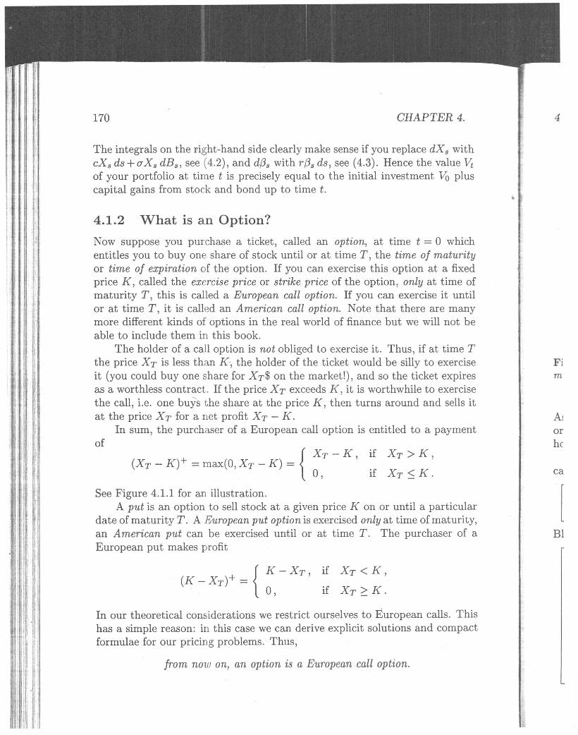
Now suppose you purchase a ticket, called an option, at time t = 0 whichentitles you to buy one share of stock until or at time T, the time of maturityor time of expiration of the option. If you can exercise this option at a fixedprice K, called the exercise price or strike price of the option, only at time ofmaturity T, this is called a European call option. If you can exercise it untilor at time T, it is called an American call option. Note that there are manymore different kinds of options in the real world of finance but we will not beable to include them in this book.

The holder of a call option is not obliged to exercise it. Thus, if at time Tthe price X T is less than K-, the holder of the ticket would be silly to exerciseit (you could buy one share for XT$ on the market!), and so the ticket expiresas a worthless contract. If the price XT exceeds K, it is worthwhile to exercisethe call, i.e. one buys the share at the price K, then turns around and sells itat the price XT for a net profit XT - K.

In sum, the purchaser of a European call option is entitled to a payment

{XT-K

(XT - K)+ = max(O, XT - K) = '0,

if XT > K,

if XT:S K.

I, I'11,1'

i '!, :

See Figure 4.1.1 for an illustration.A put is an option to sell stock at a given price K on or until a particular

date of maturity T. A European put option is exercised only at time of maturity,an American put can be exercised until or at time T. The purchaser of aEuropean put makes profit

{K -XT,

(K - XT)+ =0,

if XT < K,

if XT 2: K.

In our theoretical considerations we restrict ourselves to European calls. Thishas a simple reason: in this case we can derive explicit solutions and compactformulae for our pricing problems. Thus,

o Kq

III<XlOl

1.0 0 0.0

Figure 4.1.1 The value of a European call option with exercise price K at time ofmaturity T.

As an aside, it is interesting to note that the situation can be imagined col-orfully as a game where the reward is the payoff of the option and the optionholder pays a fee (the option price) for playing the game.

Since you do not know the price XT at time t = 0, when you purchase thecall, a natural question arises:

How much would you be willing to pay for such a ticket, i.e. what is arational price for this option at time t = 0 ?

• An individual, after investing this rational value of money in stockand bond at time t = 0, can manage his/her portfolio according toa self-financing strategy (see p. 169) so as to yield the same payoff(XT - K)+ as if the option had been purchased.'

• If the option were offered at any price other than this rational value,there would be an opportunity of arbitrage, i.e. for unboundedprofits without an accompanying risk of loss.

4.1.3 A Mathematical Formulation of the Option PricingProblem

Now suppose we want to find a self-financing strategy (at, bt) and an associatedvalue process Vi such that

for some smooth deterministic function u(t, x). Clearly, this is a restriction:you assume that the value Vi of your portfolio depends in a smooth way ont and Xt. It is our aim to find this function u(t, x). Since the value VT ofthe portfolio at time of maturity T shall be (XT - K)+, we get the terminalcondition

VT = U(O,XT) = (XT - K)+ .In the financial literature, the process of building a self-financing strategy suchthat (4.4) holds is called hedging against the contingent claim (XT - K)+.

We intend to apply the Ito lemma to the value process Vi = u(T - t, Xt).Write f(t,x) = u(T - t,x) and notice that ~

h(t,x) = -ul(T - t,x), 12(t,x) = u2(T - t,x), 122(t,x) = U22(T - t,x).

Also recall that X satisfies the Ito integral equation

Xt = Xo + e it Xs ds + (5 ltXs dEs.

Now an application of the Ito lemma (2.30) with A(1) = eX and A(2) = (5 Xyields that

f(t, Xt) - f(O, Xo)

lt

[h (s, Xs) + e Xs 12(s, Xs) + 0.5 (52 X; 122(s, Xs)] ds

+ lt[(5 Xs 12(s, Xs)] dEs

It[-U1(T - s,Xs) + eXsu2(T - s,Xs)

+ 0.5 (52 X; U22(T - s, Xs)] ds

+ it [(5 Xs u2(T - s, Xs)] dEs.o ~

On the other hand, (at, bt) is self-financing:

lit - Vo = it as dXs + it bs d(3s .

d(3t = r (30 ert dt = r (3t dt .

Moreover, lit = at Xt + bt (3t, thus

b - lit - atXtt-

(3t

Combining (4.6)-(4.8), we obtain another expression for

TT Vi t dX t Vs - asXs (3 dVt - 0 = Jo as s + Jo (3s r s s

lot ca,X,ds + lot rIa, X, dB, + lot r(V,-a,X,)ds

t[(e-r)asXs+rVs]ds + t[crasXs]dBs. (4.9)Jo ~ Jo ~ _,/' ~

Now compare formulae (4.5) and (4.9). We learnt on p. 119 that coefficientfunctions of Ita processes coincide. Thus we may formally identify the inte-grands of the Riemann and Ita integrals, respectively, in (4.5) and (4.9):

at

~r)atXt.+r~t)~ V

t

u2(T - t,Xt), (4.10)~ --(e-r)u2(T-t,XdXt+ru(T-t,Xt) ,Il) I'~.q\-ul(T - t, Xt) + eXt U'2(T - t, Xt)

+0.5 cr2xl U22(T - t, Xt) .

Since Xt may assume any positive value, we can write the last identity as apartial differential equation ("partial" refers to the use of the partial derivativesof u):

Ul(t,X) = 0.5cr2x2u22(t,X) +rxu2(t,X) -ru(t,x), (4.11)

x > 0, t E [0,T] .

(4.12) /At tim(XT -is not Eat the'In general, it is hard to solve a partial differential equation explicitly, and so

one has to rely on numerical solutions. So it is somewhat surprising that thepartial differential equation (4.11) has an explicit solution. (This is perhapsone of the reasons for the popularity of the Black-Scholes-Merton approach.)The partial differential equation (4.11) with terminal condition (4.12) has beenwell-studied; see for example Zauderer (1989). It has the e~plicit solution

u (t, x) = x <I> (g (t, x)) - K e- rt <I> ( h (t, x)) ,If we ~tmge, sstrateg:

In(x / K) + (r + 0.50-2) to-t1/2

Thus yportfolito payXT > 1the exepay an:profit i~

Thfor npself-fineopportlof loss.chaser (risks.

g(t, x) - 0- t1/2 ,

_ 1 IX _y2/2<I>(x) - (271")1/2 -00 e dy,

is the standard normal distribution function.After all these calculations,

what did we actually gain?

Recalling our starting point on p. 171, we see that

is a rational price at time t = 0 for a European call option with exerciseprice K.The stochastic process Vi = u(T -t, Xt) is the value of your self-financingportfolio at time t E [0, T].

Note~The idEbut onl

At time of maturity T, the formula (4.13) yields the net portfolio value of(XT - K)+. Moreover, one can show that at > 0 for all t E [0,T], but bt < 0is not excluded. Thus short sales of stock do not occur, but borrowing moneyat the bond's constant interest rate r > 0 may become necessary.

Equation (4.13) is the celebrated Black-Scholes option pricing formula.We see that it is independent of the mean rate of return c for the priceXt, but it depends on the volatility (J".

If we want to understand q = u(T, Xo) as a rational value in terms of arbi-trage, suppose that the initial option price p =j:. q. If p > q, apply the followingstrategy: at time t = 0

• sell the option to someone else at the price p, and

• invest q in stock and bond according to the self-financing strategy (4.14).

Thus you gain an initial net profit of p - q > O. At time of maturity T, theportfolio has value aT XT + bT fJr = (XT - K)+, and you have the obligationto pay the value (XT - K)+ to the purchaser of the option. This means: ifXT > K, you must buy the stock for XT, and sell it to the option holder atthe exercise price K, for a net loss of X T - K. If X T ::; K, you do not have topay anything, since the option will not be exercised. Thus: the total terminalpr-ofit is zero, and the net profit is p - q.

The scale of this game can be increased arbitrarily, by selling n optionsfor np at time zero and by investing nq in stock and bond according to theself-financing strategy (nat, nbd. The net profit will be n (p - q). Thus theopportunity for arbitrarily large profits exists without an accompanying riskof loss. This means arbitrage. Similar arguments apply if q > p; now the pur-chaser of the option will make arbitrarily big net profits without accompanyingrisks.

The" idea of using Browniart motion in finance goes back to Bachelier (1900),but only after 1973, when Black, Scholes and Merton published their papers,

did the theory reach a more advanced level. Since then, options, futures and,many other financial derivatives have conquered the international world offinance. This led to a new, applied, dimension of an advanced mathematical.theory: stochastic calculus. As we have learnt in this book, this theory requiressome non-trivial mathematical tools.

In 1997, Merton and Scholes were awarded the Nobel prize for economics.Most books, which are devoted to mathematical finance, require the knowl-

edge of measure theory and functional analysis. For this reason they can beread only after several years of university education! Here are a few references:Duffie (1996), Musiela and Rutkowski (1997) and Karatzas and Shreve (1998),and also the chapter about finance in Karatzas and Shreve (1988).

By now, there also exist a few texts on mathematical finance which addressan elementary or intermediate level. Baxter and Rennie (1996) is an easyintroduction with a minimum of mathematics, but still precise and with a goodexplanation of the economic background. The book by Willmot, Howison andDewynne (1995) focuses on partial differential equations and avoids stochasticcalculus whenever possible. A course on finance and stochastic calculus is givenby Lamberton and Lapeyre (1996) who address an intermediate level based onsome knowledge of measure theory. Pliska (1997) is an introduction to financeusing only discrete-time models.

A Useful Technique: Change of MeasureIn this section we consider a very powerful technique of stochastic calculus: thechange of the underlying probability measure. In the literature it often appearsunder the synonym Girsanov's theorem or Cameron-Martin formula ..

In what follows, we cannot completely avoid measure-theoretic arguments.If you do not have the necessary background on measure theory, you shouldat least try to understand the main idea by considering the applications inSection 4.2.2.

4.2.1 What is a Change of the Underlying Measure?

The main idea of the change of measure technique consists of introducinga new probability measure via a so-called density function which is ingeneral not a probability density function.