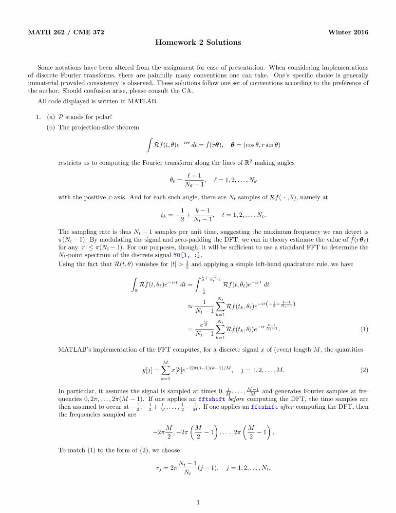
MATH 262 / CME 372 Winter 2016

Homework 2 Solutions

Some notations have been altered from the assignment for ease of presentation. When considering implementationsof discrete Fourier transforms, there are painfully many conventions one can take. One’s specific choice is generallyimmaterial provided consistency is observed. These solutions follow one set of conventions according to the preference ofthe author. Should confusion arise, please consult the CA.

All code displayed is written in MATLAB.

1. (a) P stands for polar!

(b) The projection-slice theorem ∫Rf(t, θ)e−irt dt = f(rθ), θ = (cos θ, r sin θ)

restricts us to computing the Fourier transform along the lines of R2 making angles

θℓ =ℓ− 1

Nθ − 1, ℓ = 1, 2, . . . , Nθ

with the positive x-axis. And for each such angle, there are Nt samples of Rf( · , θ), namely at

tk = −1

2+

k − 1

Nt − 1, t = 1, 2, . . . , Nt.

The sampling rate is thus Nt − 1 samples per unit time, suggesting the maximum frequency we can detect isπ(Nt− 1). By modulating the signal and zero-padding the DFT, we can in theory estimate the value of f(rθℓ)for any |r| ≤ π(Nt − 1). For our purposes, though, it will be sufficient to use a standard FFT to determine theNt-point spectrum of the discrete signal Y0[l, :].

Using the fact that R(t, θ) vanishes for |t| > 12 and applying a simple left-hand quadrature rule, we have∫

RRf(t, θℓ)e

−irt dt =

∫ 12+

1Nt−1

− 12

Rf(t, θℓ)e−irt dt

≈ 1

Nt − 1

Nt∑k=1

Rf(tk, θℓ)e−ir(− 1

2+k−1Nt−1 )

=e

ir2

Nt − 1

Nt∑k=1

Rf(tk, θl)e−ir k−1

Nt−1 . (1)

MATLAB’s implementation of the FFT computes, for a discrete signal x of (even) length M , the quantities

y[j] =

M∑k=1

x[k]e−i2π(j−1)(k−1)/M , j = 1, 2, . . . ,M. (2)

In particular, it assumes the signal is sampled at times 0, 1M , . . . , M−1

M and generates Fourier samples at fre-quencies 0, 2π, . . . , 2π(M − 1). If one applies an fftshift before computing the DFT, the time samples arethen assumed to occur at − 1

2 ,−12 +

1M , . . . , 1

2 −1M . If one applies an fftshift after computing the DFT, then

the frequencies sampled are

−2πM

2,−2π

(M

2− 1

), . . . , 2π

(M

2− 1

),

To match (1) to the form of (2), we choose

rj = 2πNt − 1

Nt(j − 1), j = 1, 2, . . . , Nt.

1

Then ∫Rf(t, θ)e−irjt dt ≈ e

irj2

Nt − 1

Nt∑k=1

Rf(tk, θl)e−i2π(j−1)(k−1)/Nt

︸ ︷︷ ︸computed with an FFT

.

We do not require a shift before applying an FFT, but we make one after in order to obtain Fourier samplesat the centered frequencies

rj = 2π

(−Nt − 1

2+ (j − 1)

Nt − 1

Nt

), j = 1, 2, . . . , Nt.

Note that f(0) is computed for each angle, as rNt2 +1

= 0, and so we can remove repeated instances. In addition,

for θNθ= π, all points are accounted for with θ0 = 0 except for the point at distance r1 = −π(Nt − 1) (so the

frequency (π(Nt − 1), 0) in the positive x-axis).

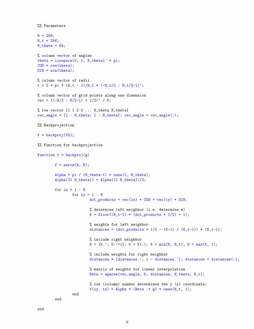
%% Parameters

N = 128;

N_t = 256;

N_theta = 64;

D = 8;

L = 4;

% maximum number of iterations in conjugate gradient

max_iter = 10;

% column vector of angles

theta = linspace(0, 1, N_theta)’ * pi;

% column vector of radii

r = 2 * pi * (N_t - 1)/N_t * (-N_t/2 : N_t/2-1)’;

% list of frequencies on polar grid

P = [0 0;

r(1) * cos(theta(N_theta)) r(1) * sin(theta(N_theta));

kron(r(1 : N_t/2), [cos(theta(1 : N_theta-1)) sin(theta(1 : N_theta-1))]);

kron(r(N_t/2+2 : N_t), [cos(theta(1 : N_theta-1)) sin(theta(1 : N_theta-1))])];

%% From Radon to Fourier via projection slice

Y1 = fftshift(fft(Y0, N_t, 2), 2) .* exp(1i * repmat(r.’, [N_theta 1]) / 2) / (N_t-1);

% value at origin

Y_origin = Y1(1, N_t/2 + 1);

% value at the one radius at angle pi not reached from angle 0

Y_pi = Y1(N_theta, 1);

% all other values

Y_else = Y1(1 : N_theta-1, [(1 : N_t/2) (N_t/2+2 : N_t)]);

% put values together, matching the order of P

Y1 = [Y_origin; Y_pi; Y_else(:)];

(c) See section 4 of the notes from Lecture 11 for the one-dimensional version of the NUFFT algorithms used inthis problem. First, the calculation

X 7→∑x∈C

Xxe−i⟨ω,x⟩, ω ∈ P (3)

2

requires a type II NUFTT. Here C is the uniform, Cartesian grid in the spatial domain, with points of the form

xn1,n2 =

(n1 +

12

N,n2 +

12

N

), n1, n2 = −N

2,−N

2+ 1, . . . ,

N

2− 1.

It will be easier to consider the finer grid C with points

xn1,n2 =( n1

2N,n2

2N

), n1, n2 = −N,−N + 1, . . . , N − 1,

and then subsample at the end. This choice is motivated by the problem’s hypothesis that Nt is twice of N ,meaning we have additional frequency data to use. We will consider a dense frequency grid D, consisting ofthe lattice

τ j1,j2 = (τj1 , τj2), τj = 2π

(−N +

j − 1

D

), j = 1, 2, . . . , 2DN.

Notice that 2πN is the maximum frequency we can compute from data on C, and is one we need sincer1 = −π(Nt − 1) ≈ −2πN . We have

f(ω) ≈ 1

(2N)2

∑x∈C

f(x)e−i⟨ω,x⟩ = Y (ω).

Taking partial derivatives of the trigonometric polynomial Y , we obtain

∂ℓ1+ℓ2

∂ℓ11 ∂ℓ2

2

Y (ω) =1

(2N)2

∑x∈C

(−ix)ℓ1(−iy)ℓ2f(x)e−i⟨ω,x⟩,

where x = (x, y). When ω = τ j1,j2 , the exponent can be written

−i⟨τ j1,j2 , x⟩ = −i2π

[x

(−N +

j1 − 1

D

)+ y

(−N +

j2 − 1

D

)]= i2π(x+ y)N − i2π

[xj1 − 1

D+ y

j2 − 1

D

].

Now

∂ℓ1+ℓ2Y

∂ℓ11 ∂ℓ2

2

(τ j1,j2) =1

(2N)2

∑x∈C

(−ix)ℓ1(−iy)ℓ2ei2π(x+y)Nf(x)e−i2π(x(j1−1)+y(j2−1))/D

If x and y are taken from 0, 12N , . . . , 2N−1

2N , these values are exactly the entries of the 2DN -point DFT (2N -pointDFT with zero-padding by a factor of D) of

1

(2N)2(−ix)ℓ1(−iy)ℓ2ei2π(x+y)Nf(x),

where j1 and j2 are allowed to vary between 1, 2, . . . , 2DN , as desired. To enforce that x and y are insteadtaken from −1

2 ,−12 + 1

2N , . . . , 12 − 1

2N , we must apply an fftshift prior to computing the FFT.

If D and L are taken sufficiently large, then for any ω = (ω1, ω2) ∈ P, we can find τ = (τ1, τ2) ∈ D close to ω.In this case, we use the approximation

Y (ω) ≈L−1∑

ℓ1,ℓ2=0

(ω1 − τ1)ℓ1(ω2 − τ2)

ℓ2

ℓ1! ℓ2!

∂ℓ1+ℓ2Y

∂ℓ11 ∂ℓ2

2

(τ ).

%% NUFFT setup

% determine the j’s corresponding to nearest neighbors

J = round(D * (P / (2*pi) + N) + 1);

% ensure 2*D*N + 1 is not one of those indices

J = min(J, 2*D*N);

3

% column of error vectors

distances = P - 2*pi * (-N + (J - 1) / D);

% compute indices when Fourier matrix on dense grid is reshaped to a column vector

J = 2*D*N * (J(:, 1) - 1) + (2*D*N - J(:, 2) + 1);

% each column (row) of x (y) is constant

vec = -1/2 + (0 : 2*N-1) / (2*N);

[x, y] = meshgrid(vec, vec);

% flip so that y coordinates ascend from bottom to top

y = flipud(y);

% padded versions of x and y, used in NUFFT_II

xx = padarray(x, [N*(D-1) N*(D-1)]);

yy = padarray(y, [N*(D-1) N*(D-1)]);

%% Type II

function Y = NUFFT_II(X)

XX = reshape(X, [2*N 2*N]);

% pad X so that nonzero entries are in the center

XX = padarray(XX, [N*(D-1) N*(D-1)]);

% initialize the column vector Y

Y = zeros(size(P, 1), 1);

for l1 = 0 : L-1

for l2 = 0 : L-1

T = fft2(fftshift((-1i*xx).^l1 .* (-1i*yy).^l2 .* exp(1i * 2*pi * (xx+yy) * N) .* XX));

% flip upside down because y-coordinate is ascending from bottom to top

T = flipud(T);

% turn matrix into a column vector

T = reshape(T, [(2*D*N)^2 1]);

Y = Y + distances(:,1).^l1 .* distances(:,2).^l2 /factorial(l1)/factorial(l2) .* T(J);

end

end

Y = Y / (2*N)^2;

end

On the other hand,

Y 7→∑ω∈P

Yωei⟨ω,x⟩, x ∈ C (4)

is a type I calculation. We adopt the process that is adjoint to the one just described. For each τ ∈ D, let

N (τ ) = {ω ∈ P : τ is the closest point in D to ω}.

4

Write x = (x, y). When ω = (ω1, ω2) is close to τ = (τ1, τ2), we can use the approximation

ei⟨ω,x⟩ = ei⟨τ ,x⟩ei⟨ω−τ ,x⟩

≈ ei⟨τ ,x⟩L−1∑

ℓ1,ℓ2=0

(ix(ω1 − τ1))ℓ1(iy(ω2 − τ2))

ℓ2

ℓ1! ℓ2!

Hence ∑ω∈P

f(ω)ei⟨ω,x⟩ =∑τ∈D

∑ω∈N (τ )

f(ω)ei⟨ω,x⟩

≈L−1∑

ℓ1,ℓ2=0

(ix)ℓ1(iy)ℓ2

ℓ1! ℓ2!

∑τ∈D

∑ω∈N (τ )

(ω1 − τ1)ℓ1(ω2 − τ2)

ℓ2 f(ω)

ei⟨τ ,x⟩.

The sum over D is the discrete inverse Fourier transform of the function Xℓ1,ℓ2 given by

Xℓ1,ℓ2(τ ) =∑

ω∈N (τ )

(ω1 − τ1)ℓ1(ω2 − τ2)

ℓ2 f(ω).

We also observe that for τ = τ j1,j2 = (τj1 , τj2),

i⟨τ , x⟩ = i2π

[x

(−N +

j1 − 1

D

)+ y

(−N +

j2 − 1

D

)]= −i2π(x+ y)N + i2π

[xj1 − 1

D+ y

j2 − 1

D

].

Therefore, in order to evaluate the discrete IFT of Xℓ1,ℓ2 onto C, we apply a 2DN -point IFFT, followed by anifftshift, and then subsample. In total,

∑ω∈P

f(ω)ei⟨ω,x⟩ ≈ e−i2π(x+y)NL−1∑

ℓ1,ℓ2=0

(ix)ℓ1(iy)ℓ2

ℓ1! ℓ2!

∑τ∈D

Xℓ1,ℓ2(τ )ei2π(x(j1−1)+y(j2−1))/D

.

%% Type I

function X = NUFFT_I(Y)

% initialize the matrix X

X = zeros(2*N, 2*N);

for l1 = 0 : L-1

for l2 = 0 : L-1

% contributions to X_{l1,l2} from nearest neighbors

S = sparse(J, 1, distances(:,1).^l1 .* distances(:,2).^l2 .* Y, (2*D*N)^2, 1);

S = reshape(S, [2*D*N 2*D*N]);

% flip upside down because y-coordinate is ascending from bottom to top

S = ifftshift(ifft2(full(flipud(S))));

% subsample back in space (middle square)

S = S(end/2 - N + 1 : end/2 + N, end/2 - N + 1 : end/2 + N);

X = X + (1i * x).^l1 .* (1i * y).^l2 /factorial(l1)/factorial(l2) .* S;

end

end

X = X .* exp(-1i * 2*pi * (x+y) * N);

5

X = reshape(X, [(2*N)^2 1]);

end

(d) Our NUFFTs allow us to approximately evaluate (3) and (4) for any signals X and Y . Call the unknownsignal f , and denote the forward transform (3) by A, and the adjoint transform (4) by A∗. Since these are

non-uniform transforms, we should not expect that A∗Af = f . Rather, we may say g = A∗f , and then tryto solve A∗Af = g for f . Since A∗A is symmetric and positive semidefinite, we can apply conjugate gradientiteration to do so. We may think of g as our naive reconstruction, stored as X1, and f (on the polar grid P) isstored as Y1.

%% Perform one iteration of type I

X1 = NUFFT_I(Y1);

X1 = reshape(X1, [(2*N)^2 1]);

%% Run pcg

f = pcg(@(x) NUFFT_I(NUFFT_II(x)), X1, [], max_iter);

f = reshape(f, [2*N 2*N]);

X1 = reshape(X1, [2*N 2*N]);

%% Display results of problem 1

figure

imshow(X1 / max(max(X1)));

figure

imshow(f / max(max(f)));

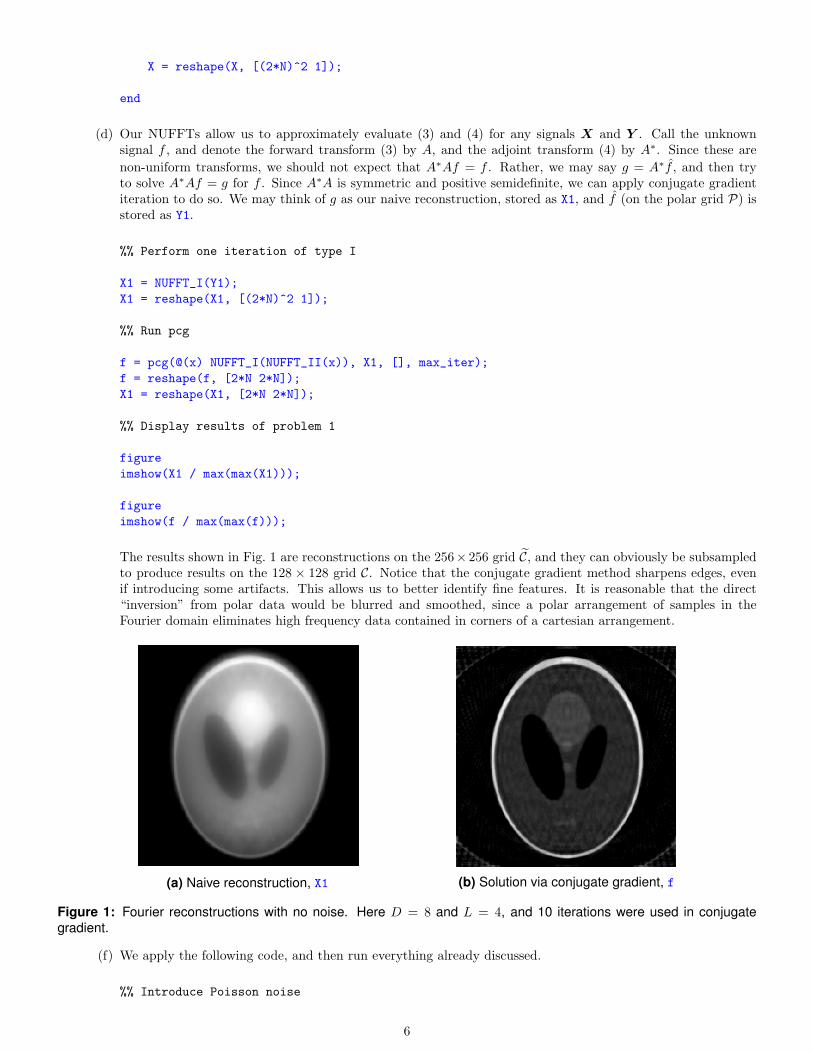
The results shown in Fig. 1 are reconstructions on the 256× 256 grid C, and they can obviously be subsampledto produce results on the 128 × 128 grid C. Notice that the conjugate gradient method sharpens edges, evenif introducing some artifacts. This allows us to better identify fine features. It is reasonable that the direct“inversion” from polar data would be blurred and smoothed, since a polar arrangement of samples in theFourier domain eliminates high frequency data contained in corners of a cartesian arrangement.

(a) Naive reconstruction, X1 (b) Solution via conjugate gradient, f

Figure 1: Fourier reconstructions with no noise. Here D = 8 and L = 4, and 10 iterations were used in conjugategradient.

(f) We apply the following code, and then run everything already discussed.

%% Introduce Poisson noise

6

lambda = 10^3 / max(max(Y0));

Y0 = poissrnd(lambda * Y0);

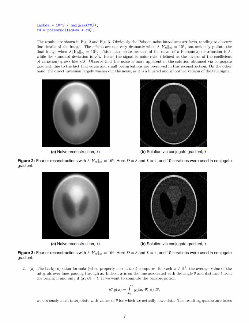
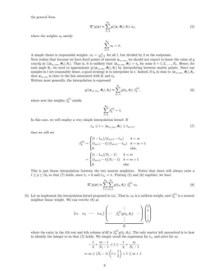
The results are shown in Fig. 2 and Fig. 3. Obviously the Poisson noise introduces artifacts, tending to obscurefine details of the image. The effects are not very dramatic when λ∥Y 0∥∞ = 106, but seriously pollute thefinal image when λ∥Y 0∥∞ = 103. This makes sense because of the mean of a Poisson(λ) distribution is λ,while the standard deviation is

√λ. Hence the signal-to-noise ratio (defined as the inverse of the coefficient

of variation) grows like√λ. Observe that the noise is more apparent in the solution obtained via conjugate

gradient, due to the fact that edges and small perturbations are preserved in this reconstruction. On the otherhand, the direct inversion largely washes out the noise, as it is a blurred and smoothed version of the true signal.

(a) Naive reconstruction, X1 (b) Solution via conjugate gradient, f

Figure 2: Fourier reconstructions with λ∥Y 0∥∞ = 106. Here D = 8 and L = 4, and 10 iterations were used in conjugategradient.

(a) Naive reconstruction, X1 (b) Solution via conjugate gradient, f

Figure 3: Fourier reconstructions with λ∥Y 0∥∞ = 103. Here D = 8 and L = 4, and 10 iterations were used in conjugategradient.

2. (a) The backprojection formula (when properly normalized) computes, for each x ∈ R2, the average value of theintegrals over lines passing through x. Indeed, x is on the line associated with the angle θ and distance t fromthe origin, if and only if ⟨x, θ⟩ = t. If we want to compute the backprojection

R∗g(x) =

∫ π

0

g(⟨x, θ⟩, θ) dθ,

we obviously must interpolate with values of θ for which we actually have data. The resulting quadrature takes

7

the general form

R∗g(x) ≈Nθ∑ℓ=1

g(⟨x, θℓ⟩, θℓ) αℓ, (5)

where the weights αℓ satisfy

Nθ∑ℓ=1

αℓ = π.

A simple choice is trapezoidal weights: αℓ =π

Nθ−1 for all ℓ, but divided by 2 at the endpoints.

Next realize that because we have fixed points of interest xn1,n2 , we should not expect to know the value of gexactly at (⟨xn1,n2 , θℓ⟩, θℓ). That is, it is unlikely that ⟨xn1,n2 , θℓ⟩ = tk for some k = 1, 2, . . . , Nt. Hence, foreach angle θℓ, we need to approximate g(⟨xn1,n2 , θℓ⟩, θℓ) by interpolating between nearby points. Since oursamples in t are reasonably dense, a good strategy is to interpolate in t. Indeed, if tk is close to ⟨xn1,n2 , θℓ⟩, θℓ,then xn1,n2

is close to the line associated with θl and tk.

Written most generally, the interpolation is expressed

g(⟨xn1,n2 , θℓ⟩, θℓ) ≈Nt∑k=1

g(tk, θℓ) β(ℓ)k , (6)

where now the weights β(ℓ)k satisfy

Nθ∑ℓ=1

β(ℓ)k = 1.

In this case, we will employ a very simple interpolation kernel: If

tm ≤ t = ⟨xn1,n2 , θℓ⟩ ≤ tm+1, (7)

then we will set

β(ℓ)k =

(t− tm)/(tm+1 − tm) k = m

(tm+1 − t)/(tm+1 − tm) k = m+ 1

0 else.

=

(t− tm)(Nt − 1) k = m

(tm+1 − t)(Nt − 1) k = m+ 1

0 else.

This is just linear interpolation between the two nearest neighbors. Notice that there will always exist a1 ≤ p ≤ Nθ so that (7) holds, since t1 = 0 and tNθ

= π. Putting (5) and (6) together, we have

R∗g(x) ≈Nθ∑ℓ=1

Nt∑k=1

g(tk, θℓ) β(ℓ)k αℓ. (8)

(b) Let us implement the interpolation kernel proposed in (a). That is, αℓ is a uniform weight, and β(ℓ)k is a nearest

neighbor linear weight. We can rewrite (8) as

(α1 α2 · · · αNt

)...

· · · β(ℓ)k g(tk, θℓ) · · ·

...

︸ ︷︷ ︸

G

11...1

where the entry in the ℓth row and kth column of G is β(ℓ)k g(tk, θℓ). The only matter left unresolved is to how

to identify the integer m so that (7) holds. We simply recall the expression for tm and solve for m:

− 1

2+

m− 1

Nt − 1≤ t ≤ −1

2+

m

Nt − 1

⇒ m ≤ (Nt − 1)

(t+

1

2

)+ 1 ≤ m+ 1.

8

%% Parameters

N = 256;

N_t = 256;

N_theta = 64;

% column vector of angles

theta = linspace(0, 1, N_theta)’ * pi;

COS = cos(theta);

SIN = sin(theta);

% column vector of radii

r = 2 * pi * (N_t - 1)/N_t * (-N_t/2 : N_t/2-1)’;

% column vector of grid points along one dimension

vec = ((-N/2 : N/2-1) + 1/2)’ / N;

% row vector [1 1 2 2 ... N_theta N_theta]

vec_angle = [1 : N_theta; 1 : N_theta]; vec_angle = vec_angle(:);

%% Backprojection

f = backproj(Y0);

%% Function for backprojection

function f = backproj(g)

f = zeros(N, N);

Alpha = pi / (N_theta-1) * ones(1, N_theta);

Alpha([1 N_theta]) = Alpha([1 N_theta])/2;

for ix = 1 : N

for iy = 1 : N

dot_products = vec(ix) * COS + vec(iy) * SIN;

% determine left neighbor (i.e. determine m)

K = floor((N_t-1) * (dot_products + 1/2) + 1);

% weights for left neighbor

distances = (dot_products + 1/2 - (K-1) / (N_t-1)) * (N_t-1);

% include right neighbor

K = [K.’; K.’+1]; K = K(:); K = min(K, N_t); K = max(K, 1);

% include weights for right neighbor

distances = [distances.’; 1 - distances.’]; distances = distances(:);

% matrix of weights for linear interpolation

Beta = sparse(vec_angle, K, distances, N_theta, N_t);

% row (column) number determines the y (x) coordinate;

f(iy, ix) = Alpha * (Beta .* g) * ones(N_t, 1);

end

end

end

9

(c) Convolution in the spatial domain is equivalent to multiplication in the Fourier domain (and vice versa). Soour strategy will be to take an FFT of g, apply the filter in the Fourier domain by multiplying by h(r) = |r|,and then compute the IFFT. From there we can just apply standard backprojection (modulo a factor of (2π)2).We have

(g( · , θℓ) ∗ h)∧

(r) = g( · , θℓ)∧

(r)h(r),

and we saw in Problem 1 that we can compute, from Radon data, Fourier samples at choice values of r:

gℓ(r) := (g( · , θℓ)∧

(rj) ≈e

irj2

Nt − 1

Nt∑k=1

g(tk, θl)e−i2πj(k−1)/Nt , (9)

rj = 2πNt − 1

Ntj, j = −Nt

2,−Nt

2+ 1, . . . ,

Nt

2− 1.

After we multiply by the filter, an inverse Fourier transform gives

(g( · , θℓ) ∗ h)(tm) ≈ 2πNt − 1

Nt

Nt2 −1∑

j=−Nt2

|rj |gℓ(rj)eirjtm

= 2πNt − 1

Nt

Nt2 −1∑

j=−Nt2

|rj |gℓ(rj)eirj(−12+

m−1Nt−1 )

= 2πNt − 1

Nt

Nt2 −1∑

j=−Nt2

|rj |gℓ(rj)e−irj/2ei2πj(m−1)/Nt (10)

Using (9) in (10), we arrive at

(g( · , θℓ) ∗ h)(tm) =1

Nt

Nt2 −1∑

j=−Nt2

|rj |

(Nt∑k=1

g(tk, θl)e−i2π(j−1)(k−1)/Nt

)ei2πj(m−1)/Nt

This is a standard FFT, followed by an fftshift to center the radii rj , followed by multiplication by |rj |,followed by an ifftshift to ensure the inverse DFT receives an input on [− 1

2 ,12 ], and then finally an IFFT

multiplied by 2π. The two shifts compose to the identity, however, and so we can equivalently shift only the|rj |. It is now easy to apply the filtered backprojection

1

(2π)2

∫ π

0

(g( · , θ) ∗ h)(⟨x, nθ⟩) dθ.

%% Function for filter

function gg = my_filter(g)

gg = fft(g, N_t, 2) .* repmat(abs(fftshift(r).’), [N_theta 1]);

gg = ifft(gg, N_t, 2) / (2*pi);

end

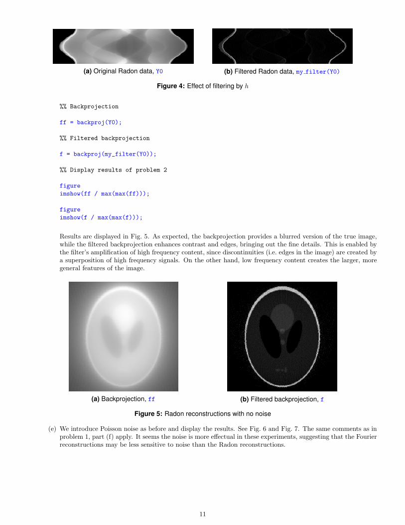
When this code is applied with g equal to Y0, we obtain filtered Radon data. The result is compared withthe original Radon data in Fig. 4. Since the visualizations display relative magnitude, we see that the highfrequency content (i.e. large t values) has now been amplified along each θ-slice. Indeed, this is clear from the

fact that h(ω) = |ω|, meaning the filter dampens low frequencies and strengthens high frequencies.

(d) We run the code presented in parts (b) and (c):

10

(a) Original Radon data, Y0 (b) Filtered Radon data, my filter(Y0)

Figure 4: Effect of filtering by h

%% Backprojection

ff = backproj(Y0);

%% Filtered backprojection

f = backproj(my_filter(Y0));

%% Display results of problem 2

figure

imshow(ff / max(max(ff)));

figure

imshow(f / max(max(f)));

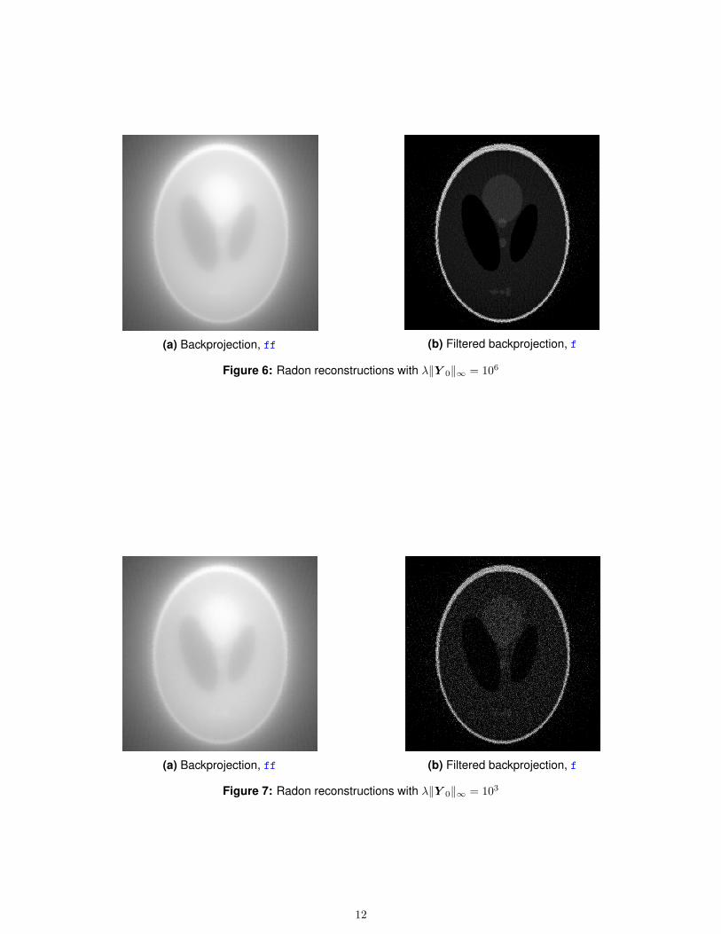
Results are displayed in Fig. 5. As expected, the backprojection provides a blurred version of the true image,while the filtered backprojection enhances contrast and edges, bringing out the fine details. This is enabled bythe filter’s amplification of high frequency content, since discontinuities (i.e. edges in the image) are created bya superposition of high frequency signals. On the other hand, low frequency content creates the larger, moregeneral features of the image.

(a) Backprojection, ff (b) Filtered backprojection, f

Figure 5: Radon reconstructions with no noise

(e) We introduce Poisson noise as before and display the results. See Fig. 6 and Fig. 7. The same comments as inproblem 1, part (f) apply. It seems the noise is more effectual in these experiments, suggesting that the Fourierreconstructions may be less sensitive to noise than the Radon reconstructions.

11

(a) Backprojection, ff (b) Filtered backprojection, f

Figure 6: Radon reconstructions with λ∥Y 0∥∞ = 106

(a) Backprojection, ff (b) Filtered backprojection, f

Figure 7: Radon reconstructions with λ∥Y 0∥∞ = 103

12