3.1

Chapter 3 Probability

3.1 INTRODUCTION

Chapter 1 addressed numbers. Chapter 2 discussed the actions that, when performed, yield numbers. In this chapter we address the third and final major concept of the triad of concepts upon which all of the remaining material in the course will depend. It is the concept of probability. Like numbers, actions and events, probability is a topic that people are exposed to on a daily basis. When the weather station forecasts a ‘30% chance of rain’, it may be re-stated as ‘the probability that it will rain is 0.3.’ When a polling agency announces that ‘70% of voters support an end to tax breaks for those making over $250,000 per year’, this claim can be re-phrased as ‘the probability that any queried voter would voice support for an end to tax breaks is 0.70’. Even the simplest example of claiming that a coin is ‘fair’, in the sense that when it is tossed the result HEADS is as likely as the result TAILS, can be stated as ‘the probability of HEADS is 0.5’.

Most readers should have been exposed to the above and other situations wherein reported numbers reflect, either directly or indirectly, probability information. It is, in fact, a main goal of almost every data collection type of study to obtain probability information in relation to the entire population. Consider the following example.

Example 1.1 Consider the following survey results from http://www.americanresearchgroup.com/economy/

August 23, 2010 Obama Job Approval Ratings Unchanged from July

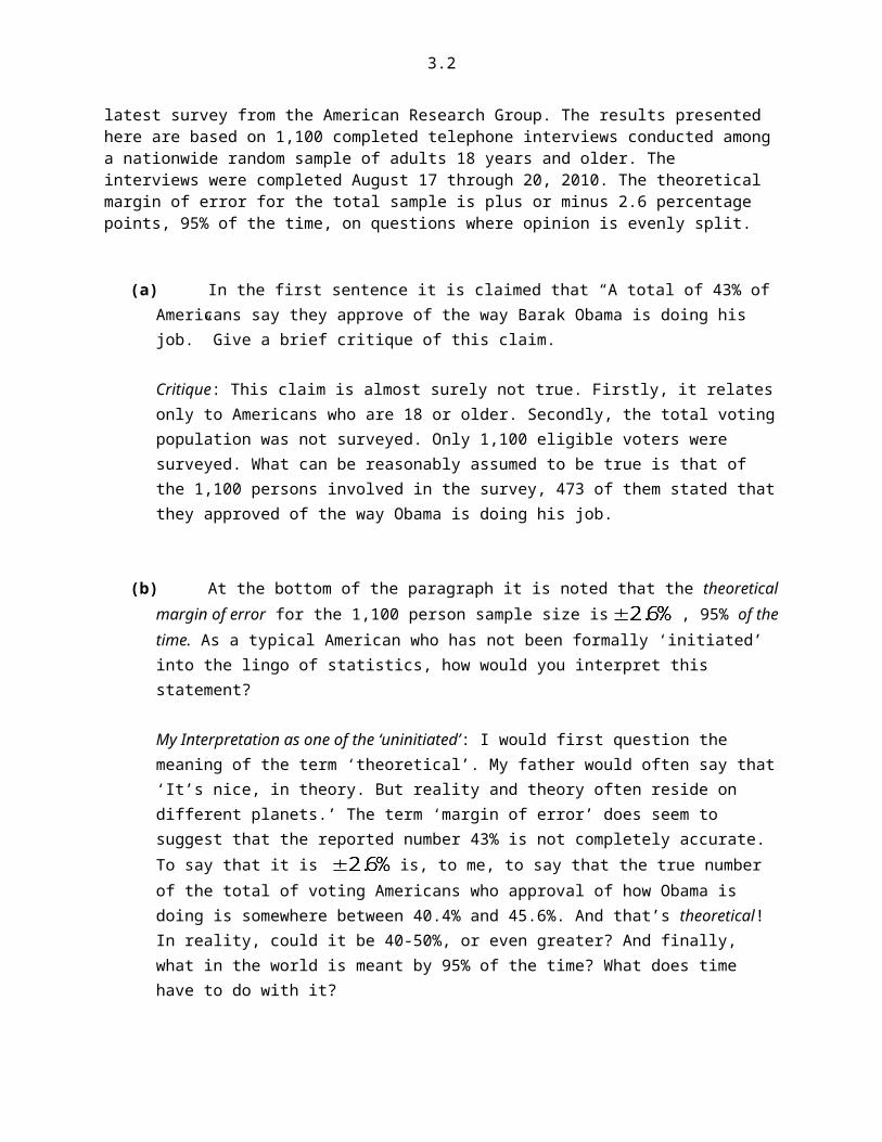
A total of 43% of Americans say they approve of the way Barack Obama is handling his job as president and 51% say they disapprove of the way Obama is handling his job (6% are undecided) according to the latest survey from the American Research Group. The results presented here are based on 1,100 completed telephone interviews conducted among a nationwide random sample of adults 18 years and older. The interviews were completed August 17 through 20, 2010. The theoretical margin of error for the total sample is plus or minus 2.6 percentage points, 95% of the time, on questions where opinion is evenly split.

(a) In the first sentence it is claimed that “A total of 43% of Americans say they approve of the way Barak Obama is doing his job.” Give a brief critique of this claim.

Critique: This claim is almost surely not true. Firstly, it relates only to Americans who are 18 or older. Secondly, the total voting population was not surveyed. Only 1,100 eligible voters were surveyed. What can be reasonably assumed to be true is that of the 1,100 persons involved in the survey, 473 of them stated that they approved of the way Obama is doing his job.

3.2

(b) At the bottom of the paragraph it is noted that the theoretical margin of error for the 1,100 person sample size is , 95% of the time. As a typical American who has not been formally ‘initiated’ into the lingo of statistics, how would you interpret this statement?

My Interpretation as one of the ‘uninitiated’: I would first question the meaning of the term ‘theoretical’. My father would often say that ‘It’s nice, in theory. But reality and theory often reside on different planets.’ The term ‘margin of error’ does seem to suggest that the reported number 43% is not completely accurate. To say that it is is, to me, to say that the true number of the total of voting Americans who approval of how Obama is doing is somewhere between 40.4% and 45.6%. And that’s theoretical! In reality, could it be 40-50%, or even greater? And finally, what in the world is meant by 95% of the time? What does time have to do with it?

(c) From (a) and (b) it should be clear that the number 43% is just an estimate of something that we don’t know. That thing can be taken to be the fraction of the total voting population that approves of Obama’s job. It can also be taken to refer to the probability that any voting American who might be asked the question would state ‘I approve’. Define the generic random variable, call it X, associated with this question. [Be sure to give its sample space.] Then express the 43% figure as a probability of a given event related to X.

Answers: X = the act of recording the response of any voting American to the question ‘How to you rate Obama’s job performance? Let the responses ‘I disapprove’, ‘I am undecided’ and ‘I approve’ be denoted as the events [X=1], [X=2] and [X=3], respectively. Then SX = {1,2,3}. It then follows that Pr[X=3] is claimed to be 0.43.

(d) Obtain a mathematical expression for the composite action that yielded the number 0.43.

Solution: As we have done on numerous previous occasions, begin by defining the 1100-D random variable where Xk = the act of recording the response of the kth

person surveyed to the question. Notice that the sample space for any Xk is exactly the same as the sample space for the generic X. Now, define generic random variable W with SW={0,1} where the event [W = 1] ~ [X = 3], and the event [W = 0] ~ . Then the random variable

denotes the corresponding survey random variables. It is then reasonable to presume that the number 0.43 was obtained from the following composite action:

.

We chose the notation because the action is an attempt to estimate the value of the true,

unknown parameter that we call .

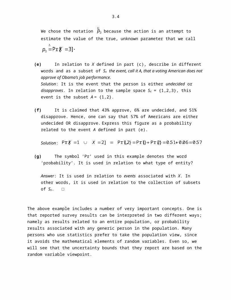
(e) In relation to X defined in part (c), describe in different words and as a subset of SX the event, call it A, that a voting American does not approve of Obama’s job performance.

3.3

Solution: It is the event that the person is either undecided or disapproves. In relation to the sample space SX = {1,2,3}, this event is the subset A = {1,2}.

(f) It is claimed that 43% approve, 6% are undecided, and 51% disapprove. Hence, one can say that 57% of Americans are either undecided OR disapprove. Express this figure as a probability related to the event A defined in part (e).

Solution:

(g) The symbol ‘Pr’ used in this example denotes the word ‘probability’. It is used in relation to what type of entity?

Answer: It is used in relation to events associated with X. In other words, it is used in relation to the collection of subsets of SX. □

The above example includes a number of very important concepts. One is that reported survey results can be interpreted in two different ways; namely as results related to an entire population, or probability results associated with any generic person in the population. Many persons who use statistics prefer to take the population view, since it avoids the mathematical elements of random variables. Even so, we will see that the uncertainty bounds that they report are based on the random variable viewpoint.

A second important concept illustrated in the above example is that the true probabilities are unknown, and so they must be estimated. How reliable the estimate is will depend on the properties of the estimator. For example, the estimator (d) of the above example used an average of 1,100 random variables. Clearly, had more subjects been included in the survey, the reported uncertainty would have been less. In the limiting case of surveying the entire voter population there would be zero uncertainty. This is neither practical, nor cost-effective, nor generally necessary, so long as the amount of uncertainty is acceptably small. Later in this chapter we will develop methods of choosing the sample size in order to achieve a specified level of uncertainty.

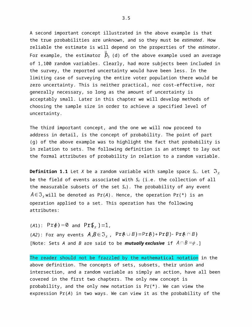
The third important concept, and the one we will now proceed to address in detail, is the concept of probability. The point of part (g) of the above example was to highlight the fact that probability is in relation to sets. The following definition is an attempt to lay out the formal attributes of probability in relation to a random variable.

Definition 1.1 Let X be a random variable with sample space SX. Let be the field of events associated with SX (i.e. the collection of all the measurable subsets of the set SX). The probability of any event

will be denoted as Pr(A). Hence, the operation Pr(*) is an operation applied to a set. This operation has the following attributes:

(A1): and ,

(A2): For any events ,

3.4

[Note: Sets A and B are said to be mutually exclusive if .]

The reader should not be frazzled by the mathematical notation in the above definition. The concepts of sets, subsets, their union and intersection, and a random variable as simply an action, have all been covered in the first two chapters. The only new concept is probability, and the only new notation is Pr(*). We can view the expression Pr(A) in two ways. We can view it as the probability of the event A, or we can view it as a measure of the ‘size’ of the set A. The reader is encouraged to view it both ways. The view of A as an ‘event’ is natural and understandable to many people who do not know about probability. The view of A as a set is mathematically expedient and concise. The view of Pr(*) as simply probability is similarly so. It is a term that most people have some qualitative understanding of. The view of it as simply a measure of the ‘size’ of a set makes it mathematically simple. The only caveat in this ‘simplicity’ is the predisposition of many people (including those in science and engineering) to view size in a narrow way. The following example is an attempt to expand the notion of size in such minds.

Example 1.2 [For those of less mathematical inclinations, this example can be skipped without any impediment to understanding of subsequent material. It is included for two reasons. First, it offers those who enjoyed calculus an opportunity to ‘re-visit an old friend’. Second, the notation associated with functions and integrals will ultimately play a role in the course material. By exposing the reader to them prior to that point, the reader who feels uncomfortable has some ‘lead time’ to brush up well before it becomes necessary to understand them.]

In this example we elaborate on the notion of Pr(*) as a measure of the ‘size’ of a set.

(a) Consider the set of all points on the non-negative real line. Call this set . Now consider the

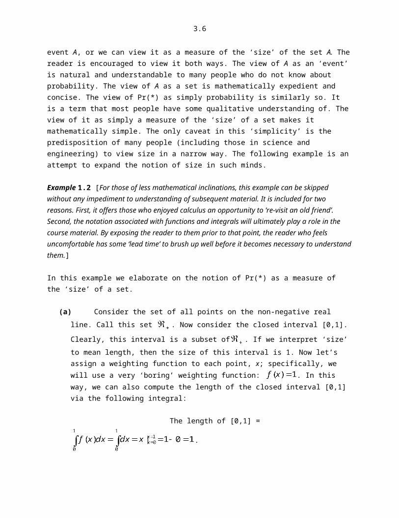
closed interval [0,1]. Clearly, this interval is a subset of . If we interpret ‘size’ to mean length, then the size of this interval is 1. Now let’s assign a weighting function to each point, x; specifically, we will use a very ‘boring’ weighting function: . In this way, we can also compute the length of the closed interval [0,1] via the following integral:

The length of [0,1] = .

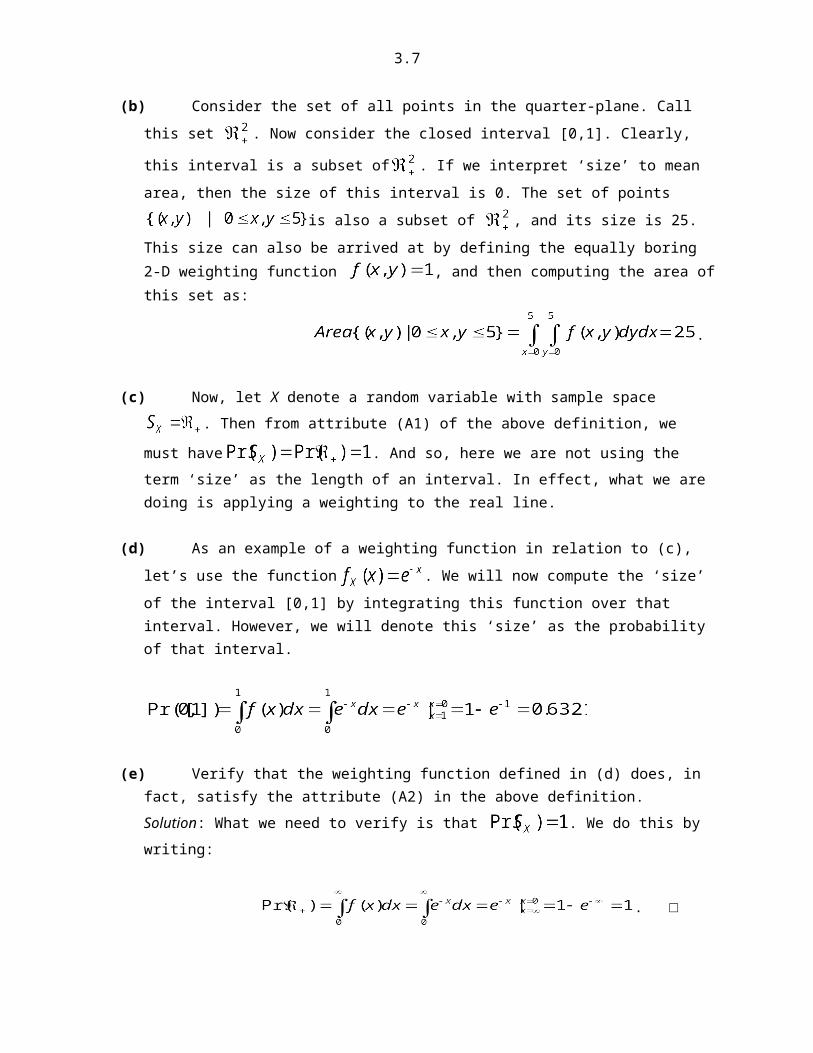
(b) Consider the set of all points in the quarter-plane. Call this set . Now consider the closed

interval [0,1]. Clearly, this interval is a subset of . If we interpret ‘size’ to mean area, then the

size of this interval is 0. The set of points is also a subset of , and its size is 25. This size can also be arrived at by defining the equally boring 2-D weighting function

, and then computing the area of this set as:

.

3.5

(c) Now, let X denote a random variable with sample space . Then from attribute (A1) of the

above definition, we must have . And so, here we are not using the term ‘size’ as the length of an interval. In effect, what we are doing is applying a weighting to the real line.

(d) As an example of a weighting function in relation to (c), let’s use the function . We will now compute the ‘size’ of the interval [0,1] by integrating this function over that interval. However, we will denote this ‘size’ as the probability of that interval.

(e) Verify that the weighting function defined in (d) does, in fact, satisfy the attribute (A2) in the above definition.Solution: What we need to verify is that . We do this by writing:

. □

The above example was mainly intended to show how Pr(*) can be viewed as measuring the ‘size’ of a subset of the sample space, or, in other words, the probability of an event. While calculus was used, readers who are nervous about calculus need not worry. Many of the applications considered in this chapter have no need of calculus. Furthermore, if the reader has questions in relation to calculus, feel entirely free to ask questions. This is not a course in calculus, and so weaknesses in that area should (hopefully) not inhibit an understanding of material central to this course. Once again it needs to be emphasized that while readers often claim that their lack of understanding is due to weaknesses in calculus and algebra, the fact is that it is basic concepts and notation that cause the biggest problems.

Before proceeding to some specific types of random variables, it is worth spending just a little time to discuss the attribute (A2) of definition 1.1. To begin, consider the Venn diagram shown below.

3.6

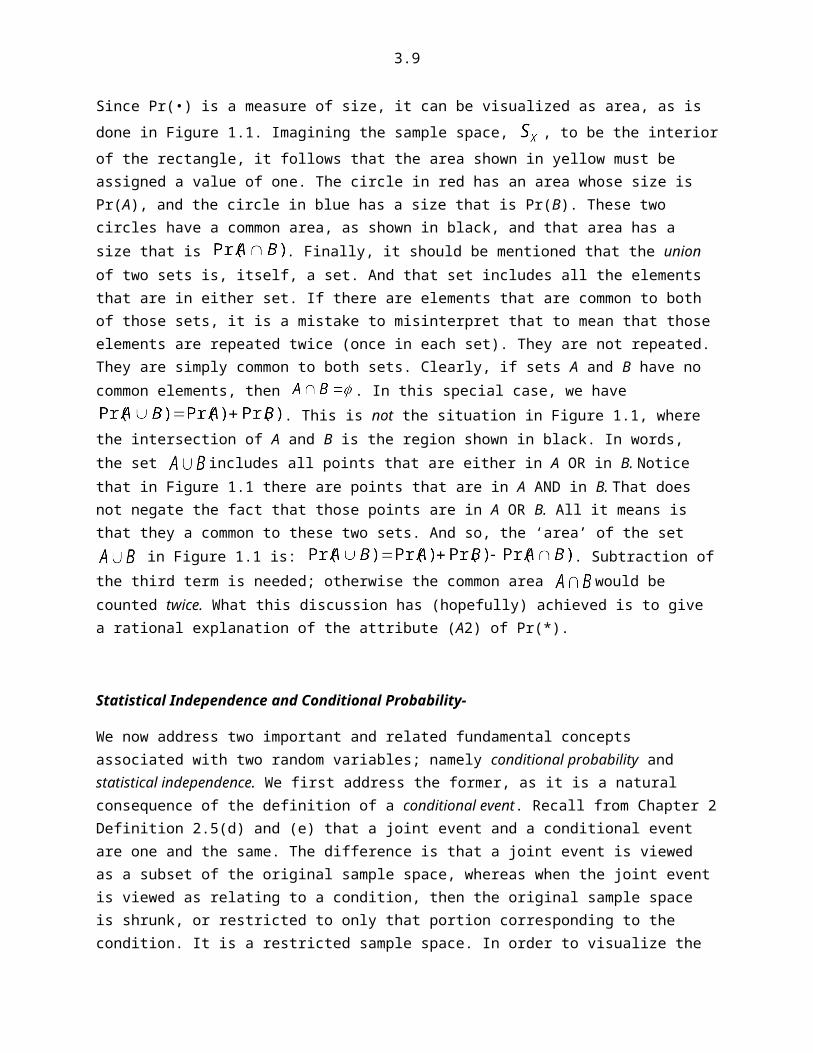
Figure 1.1 The yellow rectangle corresponds to the entire sample space, . The “size” (i.e. probability)

of this set equals one. The blue and red circles are clearly subsets of . The probability of A is the area in blue. The probability of B is the area in red. The black area where A and B intersect is equal to

.

Since Pr(•) is a measure of size, it can be visualized as area, as is done in Figure 1.1. Imagining the sample space, , to be the interior of the rectangle, it follows that the area shown in yellow must be assigned a value of one. The circle in red has an area whose size is Pr(A), and the circle in blue has a size that is Pr(B). These two circles have a common area, as shown in black, and that area has a size that is

. Finally, it should be mentioned that the union of two sets is, itself, a set. And that set includes all the elements that are in either set. If there are elements that are common to both of those sets, it is a mistake to misinterpret that to mean that those elements are repeated twice (once in each set). They are not repeated. They are simply common to both sets. Clearly, if sets A and B have no common elements, then . In this special case, we have . This is not the situation in Figure 1.1, where the intersection of A and B is the region shown in black. In words, the set

includes all points that are either in A OR in B. Notice that in Figure 1.1 there are points that are in A AND in B. That does not negate the fact that those points are in A OR B. All it means is that they a common to these two sets. And so, the ‘area’ of the set in Figure 1.1 is:

. Subtraction of the third term is needed; otherwise the common area would be counted twice. What this discussion has (hopefully) achieved is to give a rational explanation of the attribute (A2) of Pr(*).

Statistical Independence and Conditional Probability-

We now address two important and related fundamental concepts associated with two random variables; namely conditional probability and statistical independence. We first address the former, as it is a natural

3.7

consequence of the definition of a conditional event. Recall from Chapter 2 Definition 2.5(d) and (e) that a joint event and a conditional event are one and the same. The difference is that a joint event is viewed as a subset of the original sample space, whereas when the joint event is viewed as relating to a condition, then the original sample space is shrunk, or restricted to only that portion corresponding to the condition. It is a restricted sample space. In order to visualize the difference, consider the joint event that is the darkened intersection of the blue disk, A, and the red disk, B, in Figure 1.1. We can view this darkened area as a subset of the original sample space that is the yellow rectangle. Or, if we restrict our attention to only the red disk, B, we can view it as a subset of this restricted sample space.

Now, recall that any set that is defined to be a sample space must satisfy attribute (A1) of Definition 3.1; that is, its probability must be equal to 1. In the Venn diagram of Figure 3.2 we let area represent probability. Hence, the area in yellow must equal1. Clearly, the red area, which represents Pr(B) is less than 1. But if we restrict our attention to B, then we must have an area equal to 1. This necessitates that we divide Pr(B) by itself. It follows directly then, that we must scale any the probability of any subset of B by this same factor, leading to the following expression for the probability of the event A conditioned on the event B:

. (1.1)

Notice that the equality symbol in (1.1) is not a defined equality ( ). It is an equality that must hold, in

view of the condition that B is a (restricted) sample space. Attribute (A1) of Definition 1.1 requires that . If we replace the set A by the set B in (1.1), this is exactly what we get, since

. In most books on the subject the concept of conditional probability is defined by (1.1). Instead, we chose to define a conditional event. As we have stated, and will continue to state again and again, if one has a firm grasp of events, then probability is a much easier concept to grasp. To emphasize this point, we now offer the standard definition of statistical independence.

Definition 1.2 Two events A and B are said to be (statistically, or mutually) independent if

. (1.2)

With the view of Pr(*) as a measure of the size of a set, this becomes a strange definition. Referring to the Venn diagram in Figure 1.1, it states that A and B will be independent if the area of their intersection happens to equal the product of their areas. Independence requires that the intersection area be not to small, nor too large; rather, it must be just enough. We will use (1.1) routinely, since it is a very simple and convenient form. It extrapolates immediately to any number of events. For example, if events A, B, and C are mutually independent, then . It really doesn’t get much easier than that. Even so, this author feels that it lacks any intuitive appeal.

If someone says, for example, that the event that it rains in New York City today is independent of whether or not it is sunny in Delhi, most people take that to mean that the one event in no way influences the other. We can state this example in other words: Given the condition that it rains in New York City today, the probability that it will be sunny in Dehli is unaffected. With this in mind, we offer an alternative definition of independence based on conditional probability.

Definition 1.2’ Two events A and B are said to be (statistically, or mutually) independent if

3.8

. (1.2’)

This author feels that (1.2’) has much more intuitive appeal than (1.2). Granted, it requires one to have a prior understanding conditional probability. Some readers might ask how it is possible to have two different definitions of what it means for events to be independent. To those readers, we offer the following answer:

Claim The equality holds if and only if the equality holds.

Proof: First, suppose that the equality . Then (3.5) becomes . Now, suppose instead, that the equality holds. The, again from

(3.5), we obtain . □

Application to 1-D Bernoulli Random Variables- There are many phenomena that involve only two possible recordable or measurable outcomes. Decisions ranging from the yes/no type, to the success/failure type, to the good/bad type, to the right/wrong type abound in everyday life. Will I get to work on time today, or won’t I? Will I pass my exam, or won’t I? Will the candidate get elected, or not? Will my friend succeed in her business, or won’t she? Will my house withstand an earth quake of 6+ magnitude, or won’t it? Will I meet an interesting woman at the club tonight, or won’t I? Will my sister’s cancer go into remission, or won’t it. And the list of examples could go on for volumes. They all entail an element of uncertainty; else why would one ask the question. With enough knowledge, this uncertainty can be captured by an assigned probability for one of the outcomes. It doesn’t matter which outcome is assigned the said probability, since the other outcome will have a probability that is one minus the assigned probability. The act of asking any of the above questions, and then recording the outcome is the essence of what is, in the realm of probability and statistics, termed a Bernoulli random variable, as now defined.

Definition 1.2 Let X denote a random variable (i.e. an action, operation, observation, etc.) the result of which is a recorded zero or one. Let the probability that the recorded outcome is one be specified as p. Then X is said to be a Bernoulli(p) random variable.

This definition specifically avoided the use of any real mathematical notation, in order to allow the reader to not be unduly distracted from the conceptual meaning of a Ber(p) random variable. While this works for a single random variable, when we address larger collections of them, then it is extremely helpful to have a more compact notation. For this reason, we now give a more mathematical version of the above definition, using the notation developed in Chapters 1 and 2.

Definition 1.2’ Let X be a random variable whose sample space is , and let

. Then X is said to be a Bernoulli(p) random variable, or simply, a Ber(p)

random variable.

The Bernoulli random variable was chosen to be our first random variable of interest not only because it is applicable to such a wide variety of disciplines, but because it is the simplest of all random variables.

3.9

Its sample space contains only two numbers. And so the corresponding field of events is simply . Recall that Pr(*) measures the size of a set, and that the field of events is the

collection of all of the events. Hence, we see that there are only 4 events related to X: they are , , , and . In set-theoretic notation, they are the sets {0}, {1}, {0,1}, and ,

respectively.

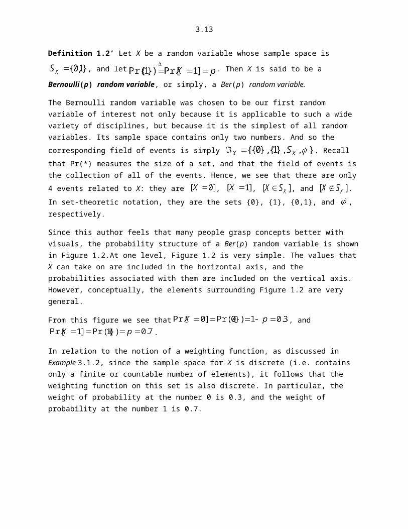
Since this author feels that many people grasp concepts better with visuals, the probability structure of a Ber(p) random variable is shown in Figure 1.2.At one level, Figure 1.2 is very simple. The values that X can take on are included in the horizontal axis, and the probabilities associated with them are included on the vertical axis. However, conceptually, the elements surrounding Figure 1.2 are very general.

From this figure we see that , and .

In relation to the notion of a weighting function, as discussed in Example 3.1.2, since the sample space for X is discrete (i.e. contains only a finite or countable number of elements), it follows that the weighting function on this set is also discrete. In particular, the weight of probability at the number 0 is 0.3, and the weight of probability at the number 1 is 0.7.

0 0.2 0.4 0.6 0.8 1 1.2 1.4 1.6 1.80

0.1

0.2

0.3

0.4

0.5

0.6

0.7

0.8

0.9

1

Pr[X

=x]

This axis includes the sample space ofr X

Figure 1.2 The probability weight function for a Ber(p=0.7) random variable.

3.2 PROBABILITY RELATED TO SINGLETON AND CUMULATIVE EVENTS FOR 1-D RANDOM VARIABLES

In Definition 2.5 of Chapter 2 we defined a number of important types of events. Some of them are only pertinent in relation to random variables of dimension two or greater. Since, here, X is a 1-D random variable, we will address only the pertinent types of events; namely singleton events and cumulative events. We repeat the definitions of these events here for convenience.

3.10

Definition 2.5(b) of Chapter 2: For any chosen , the set is called a singleton event, and is denoted as .

Notice that in the above definition we only considered a number, x, that is contained in SX. Here, we will drop this restriction and allow x to be any number on the real line, . Since X is a 1-D random variable, by definition, its sample space, SX is a subset of . Suppose that the number . Then it should be clear that is, in fact, the empty set, . This is because, since the sample space includes all possible numbers that the action X can result in, and since this number, x, is not among them, then this event can never happen. And so, from the attribute (A1) associated with PR(*), it follows that for any number we have . For the Ber(p) random variable, X, we saw in Figure 3.1.2 that only the singleton sets {0} and {1} (or, in the standard terminology, and ) have non-zero probability. When presenting Figure 3.1.2 we made no mention of the fact that, even though the horizontal axis included the real line, the only relevant numbers on the line were zero and one. We simply plotted the weights of probability at those values and let it be zero everywhere else. Readers who were comfortable with that are to be congratulated for using what this author would call ‘common sense’. The point here being that, if SX is a subset of , then one can view it as identical to , but with the caveat that any , proper, has probability zero.

Definition 2.5(a) of Chapter 2. For any chosen , the set is called a cumulative event, and is denoted as .

Here again, we will drop the restriction , and allow x to be any number in . Then, in the present case of our Ber(p) random variable, X, here are some examples of cumulative events in their standard and set-theoretic forms:

; ; ; ; ;

Notice that as the number x is increased from to , the event denoted as includes more and more of the sample space SX. The above examples of events can be generalized to the following description for a cumulative event in relation to our Bernoulli(p) random variable, X:

(2.1)

We are now in a position to explain why the cumulative event was singled out in importance. The reason is found in the following general definition.

Definition 2.1 For a 1-D random variable, X, with sample space SX, and for any chosen number , consider the cumulative event . The probability of this event is called the cumulative distribution

3.11

function for X, and is denoted as . The acronym cdf is often used to refer to the

terms ‘cumulative distribution function’.

Let’s take a moment to think about the three words in the phrase ‘cumulative distribution function’. The quantity is clearly a function of x. Moreover, it describes how probability weights are distributed over . However, the fact that this probability is in relation to a cumulative event reflects the point that it describes the accumulation of probability as a function of x.

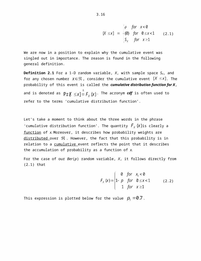
For the case of our Ber(p) random variable, X, it follows directly from (2.1) that

(2.2)

This expression is plotted below for the value .

-1 -0.5 0 0.5 1 1.5 20

0.5

1

1.5

x

F X (x)

Figure 2.1 Graph of given by (3.2) for p = 0.7.

The cdf, , allows one to compute the probability of any event associated with X. For example,

consider the event , which, in set-theoretic notation, is simply the half open interval

. This interval is half open in the sense that it includes right end point x2, but not the left end

point x1. Since is all of the probability up to, and including the number x2, and since is all of the probability up to, and including the number x1, it follows directly from attribute (A2) that the probability of this event is .

Before we proceed to some examples there is one more item that is perhaps the most popular, if not important entity associated with probability concerning a random variable, X. Even though the cdf,

, entails a complete description of any and all probability of events associated with X, it is not the most popular descriptor of the probability structure for X. The most popular entity is what we termed the

3.12

probability ‘weighting function’ in Example 3.1.2. The common term for this weighting function is given in the following definition.

Definition 2.2 For a 1-D random variable, X, with sample space SX, and cdf , the (possibly

generalized) derivative of is called the probability density function for X. It is denoted as , and the acronym pdf is often used to denote the words ‘probability density function’. In mathematical terms:

.

For readers whose background in calculus has either faded away or is still in its potential state, it is sufficient to interpret the derivative of as a function of x that describes the slope of .

In the case of our Ber(p) random variable, X, we will now compute this slope function, directly

from the plot of given in Figure 2.1. Recall that a horizontal line has a slope equal to zero. On the other hand, a vertical line has a slope that is infinite. While some more mathematically-minded readers might argue that a vertical line does not have a slope, this author prefers to view it as the limit of a sequence of lines having steeper and steeper slopes. With this point of view, it can then be said to have an infinite slope. In either case, the slope of a vertical line is not a number. Infinity is not a number. And so, with this in mind, we see from Figure 3.2 that the slope of is equal to zero for every number

. At the locations x = 0 and x = 1 the slope is infinite (or undefined). And so, properly speaking,

does not have a well-defined derivative at these points. For this reason, in relation to our Ber(p)

random variable, X, the function is said to be a generalized derivative of .

Now, while all of this may well sound very mathematical, things are not as bad as they might seem. For example, a plot of was essentially given in Figure 1.2. The term ‘essentially’ is used here because the ‘y-axis’ of the plot shows that at the location x=0 the y-value is 0.3, and at the location x=1 it is 0.7. From the above discussion we know that the value of is infinite (or undefined) at these two

locations. What the numbers 0.3 and 0.7 give is the size of the ‘jump’ in at these locations. And

so, if we were to use to arrive a plot of , we would arrive at Figure 1.2- with the understanding that the heights of the vertical lines at the locations x=0 and x=1 are not actual slope values, but rather the levels of the jumps in at those locations. In other words, those lines represent ‘lumped masses’ of probability. Stated another way:

Let X be a discrete random variable with sample space SX. Then the cumulative distribution function (cdf), is defined for ALL , and is a step function (also called a simple function). The edges

of the steps are located at points in . The height of a step at the singleton set at the point, say, , is

exactly .

3.13

3.3 THREE TYPES OF 1-D RANDOM VARIABLES

We have focused on the Ber(p) random variable in the discussion to this point. Now that we have the definition of a cumulative distribution function (cdf) and the corresponding probability density function (pdf), we are in a position to illustrate the three basic types of random variables. The Ber(p) random variable is an example of what is termed a discrete random variable. It is termed this way, since its sample space is discrete. hence, its pdf consists of lumps of probability. The following is another example of a discrete random variable

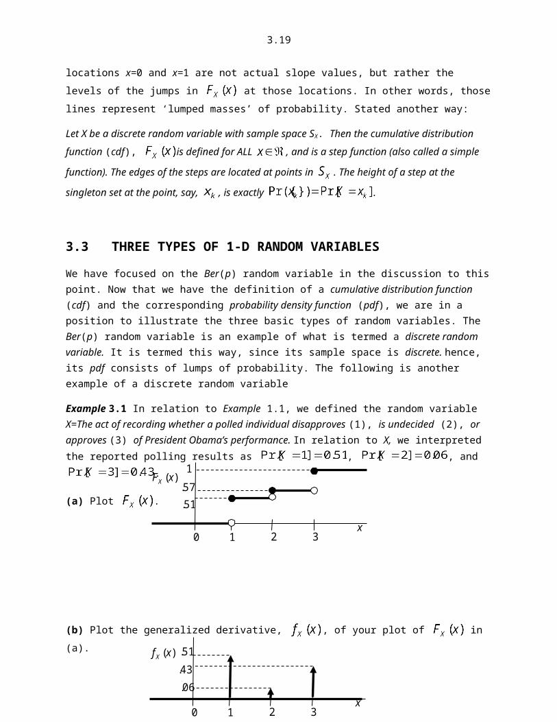
Example 3.1 In relation to Example 1.1, we defined the random variable X=The act of recording whether a polled individual disapproves (1), is undecided (2), or approves (3) of President Obama’s performance. In relation to X, we interpreted the reported polling results as , , and

.

(a) Plot .

(b) Plot the generalized derivative, , of your plot of in (a).

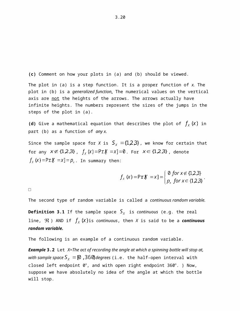
(c) Comment on how your plots in (a) and (b) should be viewed.

The plot in (a) is a step function. It is a proper function of x. The plot in (b) is a generalized function. The numerical values on the vertical axis are not the heights of the arrows. The arrows actually have infinite heights. The numbers represent the sizes of the jumps in the steps of the plot in (a).

(d) Give a mathematical equation that describes the plot of in part (b) as a function of any x.

Since the sample space for X is , we know for certain that for any ,

. For , denote . In summary then:

. □

)(xFX

1

51.57.

1x

2 30

)(xf X

43.

51.

06.

1x

2 30

3.14

The second type of random variable is called a continuous random variable.

Definition 3.1 If the sample space is continuous (e.g. the real line, ) AND if is continuous, then X is said to be a continuous random variable.

The following is an example of a continuous random variable.

Example 3.2 Let X=The act of recording the angle at which a spinning bottle will stop at, with sample space degrees (i.e. the half-open interval with closed left endpoint 0o, and with open right endpoint 360o. ) Now, suppose we have absolutely no idea of the angle at which the bottle will stop.

(a) Plot .

(b) Since is the derivative of , it follows that is the integral of . Specifically,

Here, the function . This is called the indicator function. Plot .

□

The vast majority of introductory textbooks in probability and statistics address only discrete and continuous random variables. Even so, there are many random variables that are a mix of discrete and continuous structure. The following includes an example of a mixed random variable.

)(xf X

360/1

x3600

)(xFX

1

x3600

3.15

Example 3.3 Suppose that the voltage going into the input of an audio recording device, call it V, is a

continuous random variable with sample space millivolts, and that its pdf, is flat

on this interval; that is, .

(a) Find the numerical value of c so that is a well-defined pdf.

Solution: We must have . Hence, .

(b) Find .

Solution: .

(c) Find .

Solution: .

(d) Suppose that prior to running the voltage into the recording device, it is run through a voltage limiter

box. The intent of such a box is to help prevent large voltages from damaging the recording device.

Suppose that any voltage magnitude that is greater than 5 mv is set equal to (limited to) 5 volts. Let W be

the output voltage from this box. For any event with , the box does nothing. In other

words, . However, for any , the event is equivalent to the event . Similarly,

for any , the event is equivalent to the event . Now, the sample space for W is

the continuous interval mv. Furthermore, for any , since the box does nothing, it should be

easy to see that . However, .

Similarly, . In other words, is a pdf

that is not continuous at the end points of its sample space . It has a ‘lump’ of probability equal to

0.25 at each endpoint. A comparison of and is shown in the figure below. In this case, the

formal interpretation of (3.3a) is not appropriate; nor is the use of (3.3a’). The random variable, W, is

neither a continuous, nor a discrete random variable. It is actually a mix of the two.

3.16

The above figure includes plots of and (BLUE). By running the voltage through the limiter

the grey-shaded outer rectangles, each of which has are 0.25, are transformed into lumps of probability at

the v-values volts. Clearly, W is a mixed random variable.

(e) Give a mathematical expression for .

This mathematical expression can be obtained in a manner similar to the one obtained in part (d) of

Example 3.1. However, here we must be a little more careful. Specifically, it needs to be pointed out that

for any (i.e. the open interval that does not contain the endpoints ), even though

, we have . This follows from the definition of as the derivative of

, which is a probability. In relation to the plot of , for any interval it

is the area beneath over this interval that is . In fact, we can write this probability

as

. Clearly, as we choose to be closer and closer to , this

probability will go to zero. And so, a mathematical expression for is:

.

The reader must be very careful not to compare the number 0.05 to the number 0.25. The number 0.05 is

not probability, whereas the number 0.25 is probability. □

Discussion of a more mathematical description of lumps of probability-

[Note: This remark is intended for the reader having a more mathematical persuasion. The reader who

wishes to not read this remark will not be adversely affected. ]

In the last section it was noted that if the cdf, , a random variable, X, has a step (or jump) at a

location, say , then the derivative of , which is the pdf has a slope that is at .

, of your plot of in (a). [Alternatively, one can say that is undefined at .] The

mathematical notation to describe at entails the use of the Dirac delta function. There are many ways to define this function. In fact, it is not a function at all, in the proper sense of the term ‘function’. It

3.17

is called a generalized function, in the sense that it’s integral is a proper function. Here, we will define the proper function, call it , as:

If one were to draw this function it would have a jump from the value zero to the value one at . It is a well-defined function of x. However, it is discontinuous at . Having this proper function, we will define the Dirac delta function, call it in terms of the following integral:

.

Notice that, from this definition, is equal to zero for every value . At the value , while is not well-defined, its integral, , experiences a unit jump.

Now consider the shifted Dirac delta function . This function is equal to zero for every value

. At the value , , experiences a unit jump from zero to one.

We are now in a position to give a mathematical expression for the generalized pdf for :

.

For the mixed random variable in Example 3.3 we have

. □

3.4 THE CONNECTION BETWEEN PROBABILITY AND FORCES ON A

BEAMThis section is included for the reader who has taken a course in basic physics. If you have ever played on a see-saw with a friend when you were a child (or even today!), then you might enjoy this section and discover ways of having even more fun with your friend on the other end of the see-saw.

The notion of ‘lumped masses’ is analogous to the notion of ‘point forces’ in relation to the engineering areas of statics and dynamics. To elucidate on this analogy, consider the following example of point forces acting on a beam.

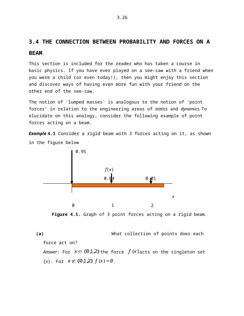
Example 4.1 Consider a rigid beam with 3 forces acting on it, as shown in the figure below

0.95

f(x)

0.04 0.01

3.18

x

0 1 2

Figure 4.1. Graph of 3 point forces acting on a rigid beam.

(a) What collection of points does each force act on?

Answer: For the force acts on the singleton set {x}. For .

(b) Give the mathematical expression for the accumulated force (or load) on the beam as a function

of x. Denote this cumulative load as L(x). Also, plot this expression.

Answer: .

1.0

0.99

L(x) 0.95

x

0 1 2

Figure 4.2. Graph of the cumulative force as a function of increasing x.

(c) Recall that pressure is defined as force applied per unit of surface area. For example, the acronym

psi refers to pounds of force per square inch. Let p(x) denote pressure. Give a mathematical

description of p(x) as a function of x.

Answer: There are many ways to describe this pressure mathematically. First we will give an

expression that is not very mathematically precise. Then we will give one that is precise. The

latter is given only for the benefit and/or curiosity of more mathematically inclined readers. We

will generally not use it.

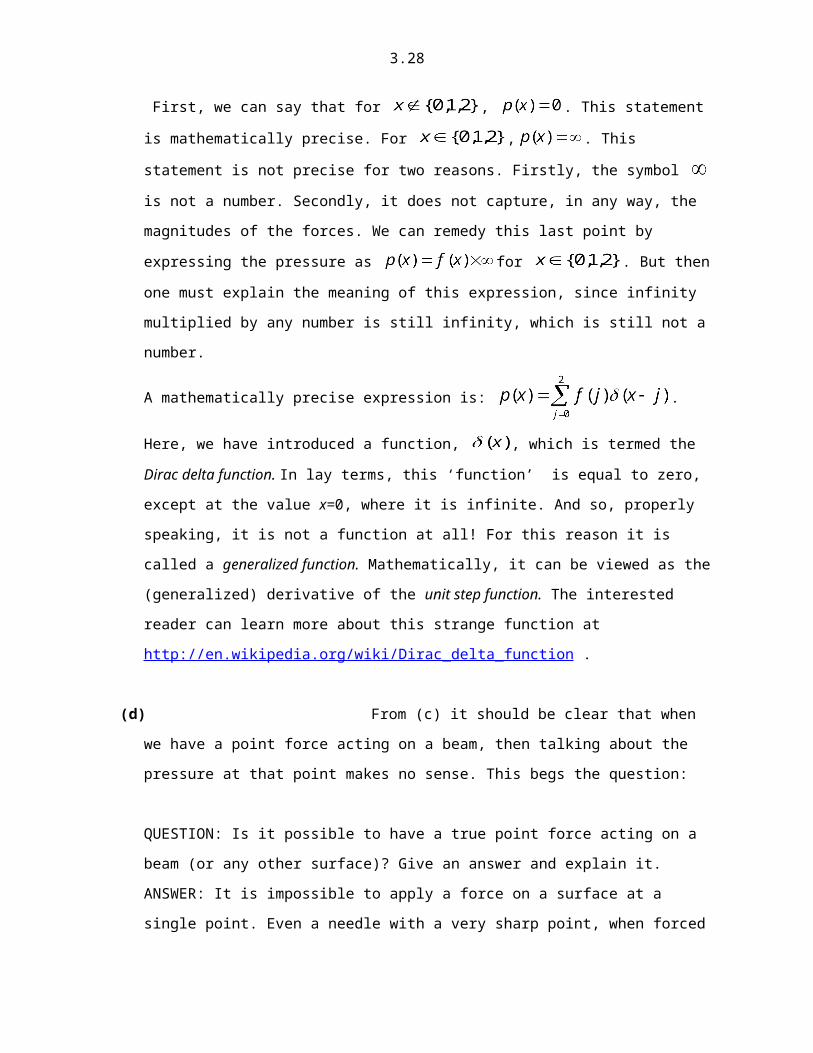
First, we can say that for , . This statement is mathematically precise. For

, . This statement is not precise for two reasons. Firstly, the symbol is not

a number. Secondly, it does not capture, in any way, the magnitudes of the forces. We can

3.19

remedy this last point by expressing the pressure as for . But then

one must explain the meaning of this expression, since infinity multiplied by any number is still

infinity, which is still not a number.

A mathematically precise expression is: . Here, we have introduced a

function, , which is termed the Dirac delta function. In lay terms, this ‘function’ is equal to

zero, except at the value x=0, where it is infinite. And so, properly speaking, it is not a function at

all! For this reason it is called a generalized function. Mathematically, it can be viewed as the

(generalized) derivative of the unit step function. The interested reader can learn more about this

strange function at http://en.wikipedia.org/wiki/Dirac_delta_function .

(d) From (c) it should be clear that when we have a point force acting on a beam, then talking about

the pressure at that point makes no sense. This begs the question:

QUESTION: Is it possible to have a true point force acting on a beam (or any other surface)?

Give an answer and explain it.

ANSWER: It is impossible to apply a force on a surface at a single point. Even a needle with a

very sharp point, when forced against a surface will contact an area; not a single point. The use of

a point force model is justified when the contact area is small relative to the total surface area,

and when ‘global’ properties are of interest. One such global property is the total force on the

beam [as was addressed in (b)]. We now address two other global properties.

(e) Compute the moment about the beam location x=0.

Answer: The term moment refers to the torque. For example, when you need to remove a lug nut

from the wheel of your car, it is easier to do it using a wrench having a long handle. This is

because you get more torque for a given amount of applied force. Torque is equal to force times

distance. And so, the moment about the location x=0 is:

(f) Notice that there is no upward pointing force in the above figure. In order for the beam to remain

in a static position there must be a total upward pointing force equal to the total downward

pointing force, which is 1.00. If a single upward force of value 1.00 is placed at the location x=0,

then, even though the forces balance, since the moment about this location is not zero, the beam

will move in a clockwise rotating fashion about this pivot point. Find the location, call it xb,

3.20

where the upward point force with value 1.00 should be located so that the moment about that

pivot point is zero.

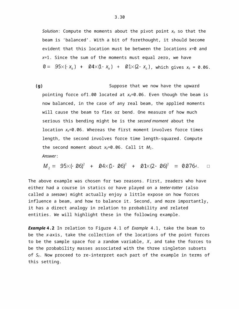
Solution: Compute the moments about the pivot point xb so that the beam is ‘balanced’. With a bit

of forethought, it should become evident that this location must be between the locations x=0 and

x=1. Since the sum of the moments must equal zero, we have

, which gives xb = 0.06.

(g) Suppose that we now have the upward pointing force of1.00 located at xb=0.06. Even though the

beam is now balanced, in the case of any real beam, the applied moments will cause the beam to

flex or bend. One measure of how much serious this bending might be is the second moment

about the location xb=0.06. Whereas the first moment involves force times length, the second

involves force time length-squared. Compute the second moment about xb=0.06. Call it M2.

Answer:

. □

The above example was chosen for two reasons. First, readers who have either had a course in statics or have played on a teeter-totter (also called a seesaw) might actually enjoy a little expose on how forces influence a beam, and how to balance it. Second, and more importantly, it has a direct analogy in relation to probability and related entities. We will highlight these in the following example.

Example 4.2 In relation to Figure 4.1 of Example 4.1, take the beam to be the x-axis, take the collection of the locations of the point forces to be the sample space for a random variable, X, and take the forces to be the probability masses associated with the three singleton subsets of SX. Now proceed to re-interpret each part of the example in terms of this setting.

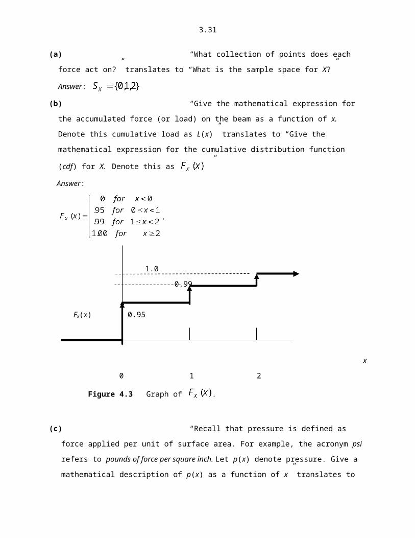
(a)“What collection of points does each force act on?” translates to “What is the sample space for X?”

Answer:

(b)“Give the mathematical expression for the accumulated force (or load) on the beam as a function of x.

Denote this cumulative load as L(x)” translates to “Give the mathematical expression for the

cumulative distribution function (cdf) for X. Denote this as ”

Answer:

.

1.0

3.21

0.99

FX(x) 0.95

x

0 1 2

Figure 4.3 Graph of .

(c) “Recall that pressure is defined as force applied per unit of surface area. For example, the acronym

psi refers to pounds of force per square inch. Let p(x) denote pressure. Give a mathematical

description of p(x) as a function of x” translates to “Give a mathematical description for the

(generalized) probability density function (pdf)”.

Answer: There are many ways to describe this pdf mathematically. First we will give an expression

that is not very mathematically precise. Then we will give one that is precise. The latter is given only

for the benefit and/or curiosity of more mathematically inclined readers. We will generally not use it.

First, we can say that for , . This statement is mathematically precise. For ,

. This statement is not precise for two reasons. Firstly, the symbol is not a number.

Secondly, it does not capture, in any way, the magnitudes of the probability masses. We can remedy

this last point by expressing the pdf as for . But then one must explain

the meaning of this expression, since infinity multiplied by any number is still infinity, which is still

not a number.

A mathematically precise expression is: .

(d) From (c) it should be clear that when we have “ a point force acting on a beam” [replace by

“probability masses”], then talking about the “pressure” [replace by “pdf”] at that point makes no

sense. This begs the question: Is it possible to have a “true point force acting on a beam” [replace by

“probability mass”] ? Give an answer and explain it.

Answer: Of course it is.

(e) Compute the moment about the “beam” [remove this word] location x=0.

Answer: The moment about the location x=0 is:

3.22

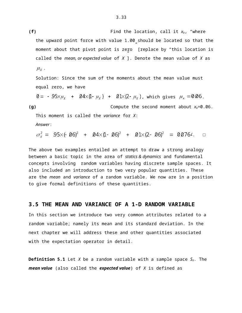
(f) Find the location, call it xb, “where the upward point force with value 1.00 should be located so that

the moment about that pivot point is zero” [replace by “this location is called the mean, or expected

value of X”]. Denote the mean value of X as .

Solution: Since the sum of the moments about the mean value must equal zero, we have

, which gives .

(g) Compute the second moment about xb=0.06. This moment is called the variance for X:

Answer:

. □

The above two examples entailed an attempt to draw a strong analogy between a basic topic in the area of statics & dynamics and fundamental concepts involving random variables having discrete sample spaces. It also included an introduction to two very popular quantities. These are the mean and variance of a random variable. We now are in a position to give formal definitions of these quantities.

3.5 THE MEAN AND VARIANCE OF A 1-D RANDOM VARIABLEIn this section we introduce two very common attributes related to a random variable; namely its mean

and its standard deviation. In the next chapter we will address these and other quantities associated with

the expectation operator in detail.

Definition 5.1 Let X be a random variable with a sample space SX. The mean value (also called the

expected value) of X is defined as

. (5.1a)

Both equalities in (5.1a) are defined equality. The left equality defines the symbol, , which is used

almost universally to denote the mean of a random variable, X. The right equality defines the expectation

operation E(*). The notation denoted the expected value of X. Sometimes it is more instructive to

express the mean value of X by the symbol . Whereas, at other times it is useful to express it as E(X).

If the sample space is continuous (e.g. the real line, ) AND if is continuous, then (5.1a) is a

formal integral. On the other hand, if is discrete, then integration, which means ‘adding things up’ just

becomes a summation operation since we no longer have a differential dx. In this case, it is common to

express the mean as:

3.23

. (5.1a’)

Remark 5.1 In this set of notes, we will use (5.1a) and (5.1a’) interchangeably for the case of a discrete

random variable. In the case of a mixed random variable, we will use exclusively (5.1a).

Definition 5.2 The variance of X is defined as

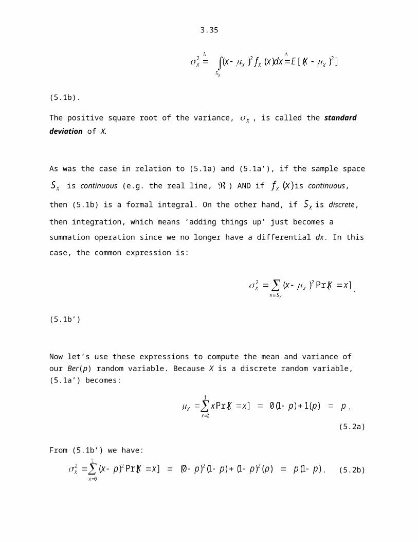
(5.1b).

The positive square root of the variance, , is called the standard deviation of X.

As was the case in relation to (5.1a) and (5.1a’), if the sample space is continuous (e.g. the real line,

) AND if is continuous, then (5.1b) is a formal integral. On the other hand, if is discrete, then

integration, which means ‘adding things up’ just becomes a summation operation since we no longer have

a differential dx. In this case, the common expression is:

. (5.1b’)

Now let’s use these expressions to compute the mean and variance of our Ber(p) random variable. Because X is a discrete random variable, (5.1a’) becomes:

. (5.2a)

From (5.1b’) we have:

. (5.2b)

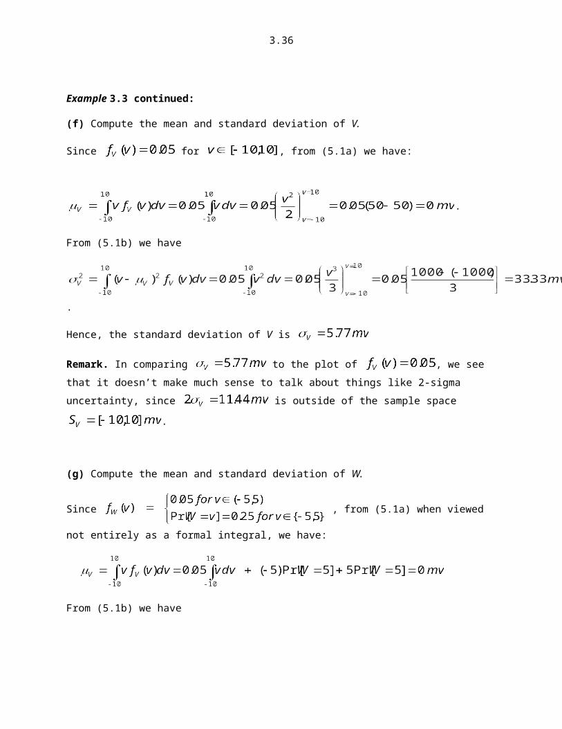
Example 3.3 continued:

(f) Compute the mean and standard deviation of V.

Since for , from (5.1a) we have:

3.24

.

From (5.1b) we have

.

Hence, the standard deviation of V is

Remark. In comparing to the plot of , we see that it doesn’t make much

sense to talk about things like 2-sigma uncertainty, since is outside of the sample space

.

(g) Compute the mean and standard deviation of W.

Since , from (5.1a) when viewed not entirely as a formal

integral, we have:

From (5.1b) we have

.

Hence, the standard deviation of W is .

Remark Even though the limiter has reduced the voltage sample space from [-10,10] to [-5,5] mv, we see that the standard deviation was reduced only from 5.77 to 4.08 mv. This relatively small reduction is due to the fact that the lumps of probability at the endpoints contribute notably to the second central moment of X (i.e. the variance). □

3.6 PROBABILITY RELATED TO 2-D RANDOM VARIABLES

We could have continued in the above development of 1-D random variables, as is done in most textbooks on the subject. While there are advantages in that route, we have chosen, instead, to embark on a discussion of 2-D random variables. The most basic 2-D random variable is the 2-D Bernoulli random

2x00p

01p

10p

11p

1x1

0

0

1

3.25

variable. We chose this route because it is a fact that the most useful and commonplace settings in statistics usually involve two or more random variables. In the 1-D setting one does not have marginal events, joint probability, covariance, and correlation concepts.

Definition 6.1. Let and be Bernoulli random variables. Then the 2-

dimensional (2-D) random variable is said to be a 2-D Bernoulli random variable with

sample space .

Since the sample space contains 4 elements, the corresponding field of events, , contains 24=16 sets or events. For notational convenience, we will denote the probabilities of the singleton events as:

.

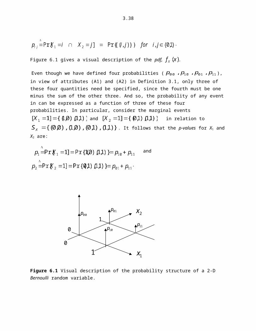
Figure 6.1 gives a visual description of the pdf, .

Even though we have defined four probabilities ( ), in view of attributes (A1) and (A2) in Definition 3.1, only three of these four quantities need be specified, since the fourth must be one minus the sum of the other three. And so, the probability of any event in can be expressed as a function of three of these four probabilities. In particular, consider the marginal events and

in relation to . It follows that the p-values for X1 and X2 are:

and .

Figure 6.1 Visual description of the probability structure of a 2-D Bernoulli random variable.

In arriving at the expressions for the p-values computed above, the concept of a marginal event as a subset of the 2-D sample space was central. Having an

3.26

understanding of these made it almost trivial to compute their probabilities. The same is true of any event one can conceive of, as is demonstrated in the following example.

Example 6.1 Let ~Ber( ).

(a) Give the set-theoretic expressions corresponding to the following events:(i) : Answer: .

(ii): : Answer: .

(iii) : Answer: .

(iv) : Answer: .

(v) : Answer: = {(0,0),(0,1)} for x1=0 and S(X1,X2) for x1=1

(vi) : Answer: = {(0,0),(1,0)} for x2=0 and S(X1,X2) for x2=1

(b) Compute the probabilities of the events in (a), in terms of .(i) : Answer: .

(ii): : Answer: .

(iii) : Answer: .

(iv) : Answer: .

(v) Pr : Answer: Pr = for x1=0 and 1.0 for x1=1

(vi) Pr : Answer: Pr = for x2=0 and S(X1,X2) for x2=1

Hopefully, the reader felt that the probabilities in the above example were almost self-evident, once the events in question were clearly described as sets. □

Example 6.2 In an effort to see whether there is any relation the failure of o-ring failures and whether or not the ambient temperature is below freezing, a sample of 40 o-rings were tested. Twenty were tested at 34oF and twenty were tested at 30oF.

(a) Define the two generic Bernoulli random variables of concern in this investigation.

3.27

Answer: Let X=the act of recording the ambient temperature. Since it is required that SX={0,1} let the event {0} ~ 34oF and the event {1} ~300F. Let Y=the act of recording whether the o-ring fails {1} or survives {0}. Then (X,Y) is a 2-D Bernoulli random variable.

(b) In relation to the sample space for (X,Y), give the set-theoretic descriptions for the following events: , , and .

Answer: ; ;

(c) The test results for the 40 o-rings are given in the table below.

Table 6.1 O-ring test results. Note that the notation ij is short for the ordered pair (i,j).

00 00 01 00 00 01 00 00 00 01 00 00 00 00 01 01 00 00 00 00

10 10 10 11 10 11 10 10 10 10 11 10 10 10 11 10 10 10 11 10

Estimate the probability of each of the three events in (b) by counting the relative number of occurrences of the appropriate event.

Answer: There are 20 occurrences of the event , 10 occurrences of the event , and 5 occurrences of the event . We will denote the true (and unknown)

probabilities of these three events as , , and

. Our relative frequency-based estimates of these are then:

, , and .

(d) Use the estimates obtained in (c) to make a claim as to whether or not the event of sub-freezing ambient temperature is independent of o-ring failure.

Answer: The event that we have a freezing ambient temperature is , and the event that we have an o-ring failure is . Theoretically, these two events are independent if the following equality holds: ; or, equivalently, if . From

(c) we found that, (lo and behold!) . Hence, we have some justification to claim that: the event of o-ring failure is independent of the event that the ambient temperature is sub-freezing.

(e) Suppose that the test results had yielded , , and

. Repeat part (d) for this situation.

Answer: Now we have and . Hence, we no longer have .

Instead, one might claim that we have , and so we can claim independence of the two events. However, this claim is a bit subjective. While one person might argue that

3.28

, another might argue that 0.125 is 25% bigger than 0.100, and that the approximate equality is not justified. The solution to this disagreement is to investigate the uncertainty of the estimators involved! □

From Definition 6.1 it was observed that the probability structure of a 2-D Bernoulli random variable, call it (X,Y), is characterized by the probabilities . Furthermore, since these must sum to 1.0, it is sufficient to know any three of these parameters in order to have complete knowledge of all four. While there are occasions in which these parameters can be addressed directly, as the last example showed, it is far more common that one addresses the marginal probability parameters and a

third parameter. In the above example that third parameter was the joint probability . In the next example we address how the various conditional probabilities associated with (X,Y) relate to these three parameters.

The Conditional Probabilities of a 2-D Bernoulli Random variable-

Let (X,Y) be a 2-D Bernoulli random variable with the marginal probability parameters and the

joint probability parameter . Let the parameter for . Then we have

the four conditional probabilities .

(a) Recall that the marginal p-values for X and Y are and . The

probabilities and are called the conditional p-

values for Y. Obtain expressions for these p-values as a function of and .

Solution: . Now, the event

is just the set , and the event is just the set . And

so: .

This gives . This, in turn, gives us the first required expression:

. (6.1a)

The second required expression is obtained far more easily:

. (6.1b)

(b) Obtain the expressions for the conditional p-values as a function of .

3.29

Solution: , (6.2a)

and

. □ (6.2b)

Some readers might be feeling a bit ‘overwhelmed’ by appearance of so much mathematics in the above example. It is recommended that those readers step through the example slowly and carefully. They will find that, in fact, there is very little mathematics- mathematics that entails only the size of a set, multiplication and division. The example uses mathematical notation. But a lack of understanding of notation does not justify the claim that the mathematics, itself, was difficult.

Example 6.2 (continued)

(f) In relation to part (c) of the example, compute estimates of the two conditional p-values for Y, compare them to the estimate of the unconditional p-value for Y, and describe them in lay terms.

Solution:

.

In words, these events state that the probability that an o-ring fails is estimated to be 0.25, regardless of whether the temperature is above or below freezing.

(g) Repeat the above for part (e) of the example. Then discuss your conclusion in relation to that associated with the Challenger space shuttle disaster :http://en.wikipedia.org/wiki/Space_Shuttle_Challenger_disaster

Solution:

.

In words, these events state that the probability that an o-ring fails, given the ambient temperature is above freezing is 0.3, which is 50% higher than the probability that it freezes, given that the ambient temperature is below freezing. This would contradict the space shuttle disaster setting, wherein it was concluded that an increased failure probability was present at below-freezing temperatures.

(h) Estimate the correlation between ambient temperature and o-ring failure.

3.30

Solution: The formula for the estimate of the theoretical correlation coefficient, call it , was given in Chapter 1, Example 1.5 part (e). The estimator (i.e. composite action) corresponding to this estimate is:

where , , and

. Applying these formulas to Table 6.1 gives the estimate

. Because this estimated correlation coefficient is close to zero, we may claim that X and Y are essentially uncorrelated. However, as we shall see, if two random variables are uncorrelated they are not necessarily independent. To be uncorrelated only means that if you were to make a scatter plot of x-y measurements, there would be no apparent orientation to the data ‘cloud’. In the case of our Bernoulli (X,Y) 2-D random variable, a data cloud would not exist since all the data would be concentrates at the four locations in the sample space. From the above analysis of the estimated conditional probabilities we had concluded that X and Y were independent. We will show that if two random variables are independent, then they must also be uncorrelated. In words, to say that X and Y are independent is basically to say that there is absolutely no relationship between them- linear or otherwise. □

In the above continuation of Example 6.2 , for a 2-D Bernoulli random variable, we addressed (i) the concept of conditional probability and how to estimate it, and (ii) the idea of the correlation coefficient and how it relates to independence. In part (h) of this example, we addressed the correlation coefficient between X and Y. In doing so, we introduced an estimator of the parameter . Some readers might be familiar with this parameter. It is called the covariance between X and Y. In Definition 3.4 we gave the expressions for the mean and variance of a random variable, X, having a discrete sample space SX. We now give the definition of the covariance, .

Definition 6.2 The covariance between 1-D random variables X and Y is defined as:

. (6.3a)

In the case where X and Y are both discrete random variables, the more common expression is:

. (6.3b)

In some textbooks a different definition of is given; specifically:

3.31

Definition 6.2’ The covariance between 1-D discrete random variables X and Y is defined as:

. (6.3b’)

Upon choosing one of the above definitions for , the other ceases to be a definition, and becomes a theorem (i.e. a fact that can be proven). Each of the expressions has its own advantages and disadvantages from a computational standpoint. In relation to a 2-D Bernoulli random variable (X,Y), the definition (6.3b’) is the easier one to compute, as we now show.

Example 6.3 Use (6.3b’) to compute the expression for . This expression should be given as a

function of the three parameters , , and .

Solution: Firstly, we have , and

. The double summation term in (6.3b’) is:

.

And so we obtain: . □ (6.4)

The calculations in the above example entailed only multiplication and addition. If the reader had difficulty following them, then it is likely that it was not the calculations, but rather the notation that is the source of the problem. Such readers are strongly encouraged to review the meaning of the notation . This symbol is simply shorthand for writing a summation of terms. It has been used many times up to this point. Equation (6.4) is noteworthy, in that it states that if and only if . But this latter equality is simply shorthand for . Hence, Bernoulli random variables X and Y are uncorrelated if and only if the events [X=1] and [Y=1] are independent events (c.f. Definition 3.7).

We need to address one final concept before proceeding to higher dimensional Bernoulli random variables, and it involves independence. As an application of Definition(s) 3.7, in part (e) of Example 3.7, we concluded that “the event that ambient temperature is below freezing” was independent of “the event that an o-ring failure will occur”. In the standard notation we can say (i): [X=1] is independent of [Y=1]. One could equally consider whether or not (ii) [X=1] is independent of [Y=0], (iii) say [X=0] is independent of [Y=1], and (iv) say [X=0] is independent of [Y=0]. Since X and Y are each Bernoulli random variables, these are the totality of events that we can pose in relation to independence. For the benefit of readers who might still have a little insecurity about the standard notation and its relation to

3.32

unabashed set-theoretic notation, let’s us the latter to arrive at conditions on the probability parameters for each of the above pair of events to be independent:

(i) independent of requires :

Translation: .

(ii) independent of requires :

(iii) independent of requires :

Translation: .

(iv) independent of requires :

Translation: .

Hopefully, those readers can better appreciate the ‘transparency’ of using set-theoretic notation. If one looks at each of the translations, it should be readily apparent, once one uses set notation, the rightmost equalities follow naturally.

Suppose that all four of the above sets of events are, indeed, independent. Then and only then can we say the following: The random variables X and Y are independent random variables. All too often people claim that two random variables are independent of each other without knowing what they are saying! By definition, the notion of independence concerns sets, not random variables. What we have just given is a definition of what it means to say that two random variables are independent. This is worthy of a formal definition.

Definition 6.3 Random variables X and Y are said to be (mutually) independent if and only if every event related to X is independent of every event related to Y.

To better appreciate why the claim of independence can be such a difficult claim to justify, consider the following example.

Example 6.4 Suppose that a subject is to answer two questions, and that the answer to each question uses a 5-point Likert scale (i.e. the possible answers are 1, 2, 3, 4, and 5). Let X=the act of answering the first question, and Y=the act of answering the second question. Determine the number of pairs of events that would need to be addressed in order to determine whether or not X and Y are independent.

Solution: Viewed alone, the sample space for X is SX={1,2,3,4,5}and the sample space for Y is SY={1,2,3,4,5}. The field of events, , related to SX has 25=32 sets. Two of these 32 sets are the ‘trivial’

3.33

set SX and . Hence, there are 30 nontrivial events contained in . Similarly, includes 30 nontrivial events. Hence, totality of possible paired events is . And so, in order to claim that X and Y are independent random variables, one needs to verify that each of the 900 pairs of events are independent. □

This author has never encountered anyone who has, or would even consider undertaking such a task as that required to ascertain the independence of such an (X,Y) random variable as was considered in the above example. It is simply way too much work! Instead, what is most commonly addressed is the correlation between X and Y. As most recently demonstrated in Example 3.7 (h), this entails computation of a single number. As it was noted, however, that number only gives one any idea of how linearly related X and Y are. It was also noted that just because X and Y are not linearly related, that does not, in general, imply that they have no type of relation to one another (a.k.a. They are independent). There are two important and very common situations where one can rightly claim that ‘because X and Y are uncorrelated, they are independent.’

Fact 6.1 Random variables X and Y that are uncorrelated, are also independent if (X,Y) is either a (i) Bernoulli, or (ii) Normal (a.k.a. Gaussian) 2-D random variable.

In this author’s opinion, the above fact is remarkable. The Bernoulli random variable is what one might call a ‘building block’ random variable. For example, EEG, which is a measure of brainwave activity, is the result of an integration of millions of synapses firings. Each synapse firing can be viewed as a Bernoulli random variable- within any specified small time interval it either fires or it doesn’t. Cancer involves the rapid growth of certain cells. A single cancerous cell presents no danger. It is a large collection of such cells that causes problems. A biopsy of tissue typically includes many cells. Each tested cell can be recorded as being either cancerous or normal. However, if one measures the degree of cancer by the cancerous fraction of a large collection of cell, the act of measuring that degree is a composite random variable that relates to a large number of Bernoulli random variables. What is equally interesting is that very often the sum (or integration of) a large number of Bernoulli random variables is a composite random variable that has a normal (or Gaussian) probability distribution. And so, in this sense, the Bernoulli and normal random variables are at opposite ends of the spectrum.

We will soon enough devote as much attention to normal random variables as were are now devoting to Bernoulli random variables. Again, we have chosen to focus first on the latter because of their simple probability structure. In keeping with this focus, we will end this section by tying together Fact 3.1, the above four requirements on for X and Y to be independent, and the expression (3.10) for the covariance between X and Y. From part (h) of Example 3.7 we note that the correlation coefficient between X and Y is defined as:

. (6.5)

It follows from (6.5) that the only way that X and Y can be uncorrelated (i.e. ) is if the covariance

between X and Y is zero (i.e. ). From Fact 3.1 we know that if then not only are X and Y

uncorrelated, they are independent. From (6.4) we know that if , then it must be that:

3.34

. (6.6)

And so, we can conclude that if (6.6) is satisfied, then X and Y are independent. Consequently, this single condition is equivalent to the totality of the four conditions on the probabilities . In other words, there is really only one condition in relation to these four parameters, and it the condition (i), namely that the events [X=1] and [Y=1] are independent.

The above discussion was not for purely ‘academic’ purposes. In fact, the expression (6.3) can give valuable practical insight into the main source of uncertainty of the covariance estimator

. To develop this insight we now proceed to address n-D Bernoulli random variables.

3.7 n-D BERNOULLI RANDOM VARIABLES

The Table 6.1 of Example 6.2 in the last section included a total of 40 paired measurements. We can denote these as . From Chapter 2, we know that there were 40 paired actions that yielded

these measurements, and that we should denote these actions as . These actions and the resulting table comprised an attempt to study the generic random variable (X,Y). And so, in words, the collection can be viewed as ‘replicates’ of (X,Y). By this we mean that each of them has the same probability structure as that of (X,Y). Making this assumption allowed us to use them to estimate a variety of probability information (marginal and conditional probabilities), and to deduce that X and Y were uncorrelated (and, in fact, independent). Imagine if we had assumed that for each 2-D measurement action , the related probability information could be different than it is for the others. We would have had no basis to use them to estimate the probability information related to (X,Y). It would have made no sense! And so, even though we were concerned with the 2-D random variable (X,Y), we, in fact, had to rely on the n-D random variables and in order to study (X,Y). Before we proceed to the more general situation where the components of the n-D Bernoulli random variable can have different p-values, let’s first consider that case where they all have one and the same p-value. We will further assume that the components are mutually independent.

Special Case #1: iid Ber(p) Random Variables- Here, we will assume that the components of the n-D Bernoulli random variable are mutually independent and identically distributed (i.e. iid), each having a Ber(pX) pdf, where the subscript in pX refers to the underlying generic random variable of interest. This is, by far, the most commonly assumed setting in relation to studies of the 1-D generic Ber(pX) random variable, X. In this setting corresponds to the n-D action of recording the responses of a ‘well-chosen’ sample. By ‘well-chosen’ we mean that each entity was chosen “at random” . The common terminology is that we have a “random sample of X”. It is so common that we will define it formally:

3.35

Definition 7.1 Let X denote a ‘generic’ random variable to be studied using a sample of n entities. The collection of measurement actions is said to be a random sample of X if each Xk has the same pdf as that of X, and if they are mutually independent. The common terminology is that they are independent & identically distributed (iid).

Notation: A comment regarding notation is appropriate. In the above definition we denoted the data collection measurement actions as a set , as opposed to an ordered n-tuple

. In the context of the definition, either notation will work. Where the notation

will fail us is when we speak of the n-D data collection action (i.e. a single 30-

dimensional action). The set is a collection of 30 actions; and it is identical to the set

, since when discussing a set or collection of objects the order of the objects is irrelevant.

Whether or not the iid assumption truly holds, it is a very ‘mathematically expedient’ (i.e. convenient) assumption. To see why, let’s first look at the consequence of the assumption of mutual independence in the simple case of the 2-D Bernoulli random variable (X,Y). In order to readily generalize this, we will use the following notation: , , . In view of Definition 6.3, the assumption that X and Y are independent results in the following equality:

[Assuming that X & Y are independent] (7.1)

In particular, (7.1) gives the following four relations:

; ; ;

.

Now, the additional assumption that the pdf for Y is identical to the pdf for X results in (7.1) becoming

[Assuming that X & Y are iid] (7.2)

And so, the above four relations become:

; ; .

Of these three relations, the middle one is telling. It tells us that it doesn’t matter what order the zero and the one are in. What counts is that there is only one 1 and one 0. We can extrapolate this point to the situation where the components of are iid with common Ber(pX) pdf:

Fact 7.1 For an n-D random variable , whose components are iid with common

Ber(pX) pdf, the pdf for is:

where . (7.3)

3.36

In word, the number y in (3.13) is the number of ‘1’s. Hence, the number n-y in (7.3) is the number of ‘0’s. Hopefully, the reader can appreciate the simplicity of the form of the pdf given by (7.3). In words, it states that for any chosen singleton subset of the sample space , it is only the number of 1’s that determines its probability.

Recall that, generally, the goal is to use then data collection random variables to better understand the probability structure of the underlying generic random variable, X. When X is a Ber(pX) random variable it’s probability structure is so simple that we need only know the value of pX to know everything about that structure, as it has a lump of probability, on the set {1}, and a lump of probability on the

set {0}. We have seen on numerous occasions to this point, that a logical estimator of , based on

is:

. (7.4a)

For the measurements , (3.14) becomes the estimate

. (7.4b)

Hence, if the reader has not yet figured it out, we have been using the term estimator to refer to a composite action (random variable) that serves as an estimator of a parameter. The term estimate, as illustrated in (7.4b), refers to a number that serves as the numerical estimate of the parameter.

Since the true mean of X is , it is entirely reasonable that we should use the sample mean (7.4) as an estimator of it. We are now finally in a position to compute the pdf of the estimator (7.4) in the situation where the components of are iid.

Development of the pdf for the estimator .

This development is quite simple if we focus on sets rather than on probability. To begin, we will first

consider the random variable . Clearly, . Consider the event that in

standard notation is . In set notation it is just {0}. This subset of SY is equivalent to the subset of which is {(0,0,…,0)}. Since these sets are equivalent, they must have the same probability. And so, we

have . Similarly, the event is equivalent to the subset of which is {(1,1,

…,1)}. And so, .

3.37

Next, consider the event , which, in words, is the event that an n-tuple includes

one 1 and n-1 0’s. The subset of that is equivalent to the event is therefore:

. This set has n distinct elements in it, and the

probability of each element, when viewed as a singleton set, is . Furthermore, the n singleton sets whose union is the set in question are mutually exclusive set; that is, the intersection of any two of them is the empty set. For example, . [Some readers may feel that the intersection cannot be the empty set, since each of these ordered n-D numbers have zeros in common in the third through the nth positions. Those readers need to return to Chapter 1 and read it again. To use an analogy, suppose we have two persons. We will classify each person using (height, weight, eye color). We will declare to persons to be one and the same person if they have the same height, weight, and eye color. Suppose these persons have the same height and weight, but one has brown eyes and the other has blue eyes. Then, by definition we have two different persons.]

Hence, we have: . Similarly, . Now, in

relation to the event , the equivalent event is, in words, the event that an n-tuple includes y ‘1’s and n-y ‘0’s. And so, the question that needs to be answered is: how many such entities are in the equivalent subset of . The answer to this question begins by answering a similar question:

How many ways can one order n distinctly different objects in n slots?

Answer: In the first slot we can place any one of the n distinct objects. Once we have chosen one of them, then in the second slot we have only distinct objects to choose from. Having chosen one of them, we are left to choose from distinct objects to place in the third slot, and so on. Think of this as a tree, where each branch has branches, and each of those branches has branches, and so on. The question is to figure out how many total branches there are. Let’s identify the first slot with the biggest diameter branches. Then we have n of these, corresponding to the n distinct objects. Now, each one of these main branches has branches of slightly smaller diameter. And each one of those branches has slightly smaller branches, and so on. So, the total number of branches is

(read as “n factorial”)

The next question that needs to be answered is:

How is the number n! reduced, in view of the fact that the y ‘1’s all look the same, and the n-y ‘0’s all look the same?

Answer: If each of the y ones and the zeros were distinctly different (say, different colors, or different aromas!), then there would be n! possible ways to order them. However, all the ones look alike, and all the zeros look alike. And so there will be fewer than n! ways to order them. How many fewer? Well, how many ways can one order the y ones, assuming they are distinct? The answer is y! ways. And

3.38

how many ways can one order zeros, assuming they are distinct? The answer is ways. But since the ones and zeros are not distinct, the number of ways we can position them into the n slots is:

(read as “n choose y” ). (7.5)

A point of notation is required in relation to (7.5), and, in particular, as to the meaning of 0!. Logically, one might reasonably expect that 0! = 0. However, if that were the case, then (7.5) would be flawed, since we know for certain that there is only one way to place 15 indistinguishable ‘0’s into 15 slots. But if we read 0! As 0, then (7.5) would yield . Hence, alas, reason fails here. Instead, the quantity 0! Is defined to equal 1. Using this definition, then in the case of 15 ‘0’s we get

. We get the same result in the case of 15 ‘1’s. In the case of 14 ‘0’s (or 14 ‘1’s) we get , which is consistent with our knowledge that there are 15 way to

place a single ‘1’ in 15 slots. And so, we have the formula for the pdf for :

. (7.6)

Since , the sample space for is .

Moreover, the singleton subset {y/n} of this sample space is equivalent to the singleton subset {y} of the sample space SY. And so the pdf of the estimator is:

(7.7)

The pdf (7.7) is a very popular one; so popular, that it has a name:

Definition 7.2 The probability distribution given by (3.16) is called a Binomial(n,pX) distribution.

And so, we have the following fact.

Fact 7.2 Given a collection, , of iid Bernoulli(pX) random variables, the composite

random variable has a Binomial(n,pX) distribution.

The mean and variance of Y are given by

Then mean (or expected value) of Y: (7.8a)

3.39

The variance of Y: (7.8b)

The mean and variance of are given by

Then mean (or expected value) of : (7.9a)

Then variance of : (7.9b)

The equalities in (7.8) will be derived in the next chapter. In that chapter we will also show how (7.9) results from (7.8). At this point however, it is important to understand what (7.9) says about the estimator,

, of the unknown parameter . The fact that the mean of is equal to is a necessary condition

for any good estimator. The fact that the variance of can be made as small as desired by choosing a suitably large sample size, n, is a second necessary condition for any good estimator.

Example 7.1 Suppose that in reforestation project it is desired to re-populate the area with 10 trees. Suppose that each seed that is planted has 20% chance of not germinating. Determine how many seeds should be planted in order that the probability that at least 10 seed germinate is 0.95.

Solution: Before getting too involved with (and overwhelmed by) all the numbers, first imagine the actions that need to be performed. A total of n seeds will be planted. Let the event denote the

event that, in words, is that the seed germinates. We then have the n-D action . The

composite action is the act of recording how many seeds will germinate.

Having the action , what do we know about each Xk? We know that it is a Bernoulli

random variable with p-value . What do we know about the joint probabilities? If

the answer is ‘nothing’, then we should assume that they are mutually independent. It follows that Y has a Binomial distribution with parameters n and . We are now in a position to formulate the mathematical problem statement:

Find the smallest value of n, such that . This statement can be re-phrased as:

Find the smallest value of n, such that . We prefer this phrasing because the event is a cumulative event, and so is the cumulative distribution function (cdf) for

Y, evaluated at y=9. And so, we have yet another formulation of the problem statement:

For Y ~ Binomial(n,pk=0.8) find the value of n such that .

To solve this problem, we will use Matlab; specifically, the command:

BINOCDF Binomial cumulative distribution function.

11 12 13 14 15 16 17 18 19 200

0.1

0.2

0.3

0.4

0.5

0.6

0.7

Number of Seeds Planted, n

F Y (9)

3.40

Y=BINOCDF(X,N,P) returns the binomial cumulative distribution function with parameters N and P at the values in X. x=9;p=0.8;for n = 11:20y(n-10) = binocdf(x,n,p);endnvec = 11:20plot(nvec,y,’*’)gridxlabel(‘Number of Seeds Planted, n’)ylabel(‘F_Y(9)’)

From the plot, we see that the required value is n = 16.

Remark 7.1: We just solved what, in a first course in statistics would generally be viewed as a very difficult problem. Our approach to solving it was to begin with the actions, and go from there. That we needed to use Matlab only emerged at the very end of the development. Had we been forced to do the computations by hand, the problem would have, indeed, been painstaking. It should be emphasized that this was a real-world problem. It was not the typical ‘use the formula to plug-and-chug’ type of problem that one typically encounters as an introductory problem in textbooks used in a first course in statistics. If the reader had no trouble following the steps in the problem formulation, then he/she is to be congratulated! In this case, the material up to this point has served its purpose. As a final note, we will continue to pose such real-world problems throughout the course. When they have been suitably re-formulated into a clear problem statement, we will often then have to appeal to Matlab commands in the Statistics Toolbox that can solve them. □

Example 7.2 Suppose that we desire to construct a section of wrought iron railing, and that it is known from past records that the probability that any given weld will fail is 0.03. Each vertical spindle will be welded at two locations; namely at the top and bottom rails.

(a) Determine the probability of achieving 16 consecutive good welds.

Solution: Consider the action , where the event denotes the event that the kth

weld fails. Let . Then .

(b) Determine the probability of achieving 10 consecutive good welds.

Solution: Consider the action , where the event denotes the event that the kth

weld fails. Let . Then .

(c) Determine the number of good welds, n, such that their probability is 0.9

3.41

Solution: Consider the action , where the event denotes the event that the kth

weld fails. Let . Then

. Hence, the condition that an integer number of n consecutive good welds have probability 0.9 requires no more than 3 welds.

(d) Suppose that a section of railing is required to have 8 spindles, and that the probability that none of the 16 welds will fail is required to be 0.95. Find the required probability,1- p, that any given weld will fail.

Solution: Consider the action , where the event denotes the event that the kth

weld fails. Let . Then . Hence, the

required probability that any given weld will fail is , or 0.3%. □

Example 7.3 In this example we will address the generic problem of patching together a sequence of 10 objects to obtain a ‘string’. Suppose that the probability that any given object has a flaw is p. The string is deemed ‘acceptable’ if the following two conditions are satisfied: (C1) there can be no more than 2 flaws, and (C2) the flaws cannot be adjacent to one another. Fin the expression for the probability that a string will NOT be acceptable.

Solution: As the reader might suspect, we will begin by determining the event that, in words, is that a string is acceptable. To this end, we have the following acceptable sets:

A = {(0,0, … , 0)} = no flawsB = {(1,0, … , 0) , (0,1,0 … , 0) , … , (0, … , 0,1)} = one flaw. N(B) = 10C1 = {(1,0,1,0…,0) , (1,0,0,1,0,…,0) , … , (1,0,…,0,1)} 2 flaws with first in position #1. N(C1) = 8.C2 = {(0,1,0,1,0…,0) , (0,1,0,01,0,…,0) , … , (0,1,…,0,1)} 2 flaws with first in position #2. N(C1) = 7.…C8 = {(0,0…,01,0,1)} 2 flaws with first in position #8. N(C1) = 1.

This was the ‘hard’ part. The easy part is now to compute the probability of each event, and add these up:

; ;

; … ; .Hence:

Pr(acceptable) = .

The above expression isn’t very ‘attractive’. And so, let’s consider a complementary alternative formulation. Let’s identify the sets that comprise the event that the string is NOT acceptable. Then we will subtract the probability of this set from 1.0.

3.42

A = the event that there are 3 or more flaws.B = the event that there are exactly two flaws and they are adjacent.

Now, Pr(A) = 1 – Pr(less than or equal to 2 flaws) = .

B = {(1,1,0…,0),(0,1,1,0,…,0),…,(0,…,0,1,1)} ; N(B) = 9. And so.

Hence, Pr(NOT acceptable) = , or

Pr(acceptable) = 1 – Pr(NOT acceptable) = .

Remark 7.2: This example was intended to once again highlight the value of a firm understanding of actions and the sets they can generate. The actions involved iid Bernoulli random variables, but not in a setting that we have addressed to this point. Nonetheless, once we had identified the sets corresponding to the events that were stated in words, it was straightforward to compute the mathematical expressions for their probabilities. The fact that these expressions did not reduce to ‘neat and clean’ simple ones is not only irrelevant, but a fact of many real world problems. What is relevant is that we have expressions; ones that can be evaluated for a variety of numerical values of the parameters (in this case, p and n) using Matlab or some other software.

Remark 3.13.2: This example also highlighted the fact that, as is often the case, there is more than one way to attack a problem. In this particular situation we first approached it by focusing on the sets corresponding to an acceptable string. Then we proceeded to focus on the sets corresponding to an unacceptable string, in the hopes that things might get a bit easier. The former approach was straightforward, but resulted in a, perhaps, unpleasant mathematical expression. The latter approach involved far fewer sets, but led us to invoke the cdf of a Binomial random variable. Both approaches have advantages and disadvantages. A key value in using different approaches is that they can be used to cross-validate the answers. If significantly different approaches yield the same answer, one can have greater confidence in its correctness. □

Before proceeding to the next section, the reader might be interested to know that in Example 3.12 we essentially introduced another random variable that relates to n iid Bernoulli random variables.

Definition 7.3 Let denote an ∞-D Bernoulli random variable, whose components are iid. The random variable, Y, that, in words, is the act of recording the position of the first occurrence of a ‘1’, is called a geometric random variable.

Clearly, a geometric random variable, Q, is a 1-D random variable, and its sample space is SQ={1,2,…, ∞}. The pdf for Q is: where p=Pr[X=1]. (7.10)

3.43

Example 7.2 continued. In part (a) of this example we computed the probability of achieving 16 consecutive good welds as: .

(e) Compute the probability that the first bad weld will occur at weld #17.

Solution: in relation to this is the singleton set , It is equivalent to the event [Q=17] where Q is a geometric random variable with p=0.03. And so, (3.20) gives

.

(f) Compute the probability that the first 16 welds are good AND the 17th weld is also good.

Solution: This is simply

(g) Use the results of (e) and (f) to verify the answer in (a).

Solution: In relation to , the event that, in words is the act of recording 16 good welds is the set . And so

. This number is essentially equal to 0.6143. □

3.8 THE CENTRAL LIMIT THEOREM IN RELATION TO

8.1 Using a Random Number Generator to Simulate n-D iid Bernoulli Random Variables

In this section we address the problem of simulating data associated with a Bernoulli random variable. This simulation will utilize a uniform random number generator. And so, first, we will formally define what we mean by a uniform random number generator.

Definition 8.1 A uniform random number generator is a program that, when called, produces a “random” number that lies in the interval [0,1].

In fact, the above definition is not very formal. But it describes in simple terms the gist of a uniform random number generator. The following definition is formal, and allows the generation of n numbers at a time.

Definition 8.1’Define the n-D random variable where each is a random

variable that has a uniform distribution on the interval [0,1], and where these n random variables are mutually independent. The two assumptions that these variables each have the same distribution and that they are mutually independent is typically phrased as the assumption that they are independent and identically distributed (iid). Then U is an n-D uniform random number generator.

3.44

The following example uses the uniform random number generator in Matlab to demonstrate this definition.

Example 8.1 Here, we give examples of an n-D uniform random variable, U, using the Matlab command “rand”, for n=1,2 and 25:

(i) U = rand(1,1) is a 1-D uniform random variable. Each time this command is executed, the result is a “randomly selected” number in the interval [0,1]. For example:

>> rand(1,1)ans = 0.9501

(ii) U=rand(1,2) is a 2-D uniform random variable. For example,

>> rand(1,2)ans = 0.2311 0.6068

(iii) U=rand(5,5) is a 25-D uniform random variable. For example,

>> rand(5,5)ans = 0.3340 0.5298 0.6808 0.6029 0.0150 0.4329 0.6405 0.4611 0.0503 0.7680 0.2259 0.2091 0.5678 0.4154 0.9708 0.5798 0.3798 0.7942 0.3050 0.9901 0.7604 0.7833 0.0592 0.8744 0.7889

It is important to note that the command rand(m,n) is the -D random variable. The numbers are a result of the command. They are not random variables. They are numbers. A random variable is an action, algorithm, or operation that when conducted yields numbers.

We now proceed to show how the uniform random number generator can be used to simulate measurements of a Bernoulli random variable. Let’s begin with a 1-D random variable. Again, we will use Matlab commands to this end.

Using U to arrive at : For , define the random variable, X, in the following way: Map the interval to the event [X=0], and map the event [ to the event [X=1]. Recall from Example 3 above that . Hence, it follows that

. Therefore, since X can take on only the value zero or one, we have ; that it, X is a Ber(p) random variable. Here is a Matlab code that corresponds to :

p=0.7;u=rand(1,1);

3.45

if u <=1-px=0elsex=1end

For example:

>> p=0.7;u=rand(1,1);if u <=1-px=0elsex=1endx = 1

A NICE TRAIT OF MATLAB:

Now, suppose that we want to simulate multiple measurements associated with this random variable associated with the above code. Well, we could simply embed the code in a DO loop, and

repeat the above operation the desired number of times. Well, it turns out that Matlab is a programming language that is not well-suited to DO loops. If the loop count is small, it works fine. But if you wanted to simulate, say one million values associated with X, then it would take a long time. In fact, Matlab was designed in a way that makes it a very fast code for batch or vector operations. With this in mind, the code below is offered. It includes no IF/ELSE commands, and it requires no DO loop for multiple measurements. We will give the code for the case of one million values associated with X.

p=0.7;m=1000000;u=rand(1,m);u=u-(1-p);x=ceil(u);

The command u=rand(1,m) results in a 1x1000000 vector of numbers between 0 and 1. The command u=u-(1-p), shifts every number to the left by an amount 1-p. Thus, since here p=0.7, every number that was in the interval [0,0.3] has been shifted to a number in the interval[-0.3,0]. In particular, not only is every such number now a negative number, but the closest integer to the right of it is zero. The ceil command rounds numbers to the next higher integer. The command ceil is short for ceiling, or “round up to the nearest integer”. Similarly, numbers originally in the interval (0.3,1] are moved to the interval (0,0.7]. Since they are still positive, the next highest integer associated with them is one. Here is an example of running the above code. Rather than showing x, which contains one million zeros/ones, we included a command that adds these numbers. This sum is the number of ones, since zeros contribute nothing to a sum.

3.46

>> p=0.7;m=1000000;u=rand(1,m);u=u-(1-p);x=ceil(u);>> sum(x)

ans = 700202

Notice that the relative frequency of ones is 700202/1000000, which is pretty close to the 0.7 p-value for X. In fact, if we were to pretend that these numbers were collected from an experiment, then we would estimate the p-value for X by this relative frequency value. The value of running a simulation is that you know the truth. The truth in the simulation is that the p-value is 0.7. And so, the simulation using 1000000 measurements appears to give a pretty accurate estimate of the true p-value. We will next pursue more carefully what this example has just demonstrated.

Using to Simulate Independent and Identically Distributed (iid) Ber(p) Random Variables, and then, from these, investigating the probability structure of the random

variable .

In this subsection we are interested in using simulations to gain some idea of how many subjects, n, would be required to obtain a good estimate of the p-value of a typical subject. The experiment is based on the question: What is the probability that a typical American believes that we should withdraw from Iraq. We will identify the set {1} with an affirmative, and the set {0} with opposition. We will ask this question to n independent subject and record their responses. Let be the response of the kth subject. Notice that we are assuming that each subject has the same probability, p, of believing that we should withdraw. Thus, is an n-D random variable whose components are iid Ber(p) random variables. After we conduct the survey, our next action will be to estimate p using the estimator

. (8.1)

Notice that (8.1) is a random variable that is a composite action that includes first recording the responses of n subjects, and then taking an average of these responses.

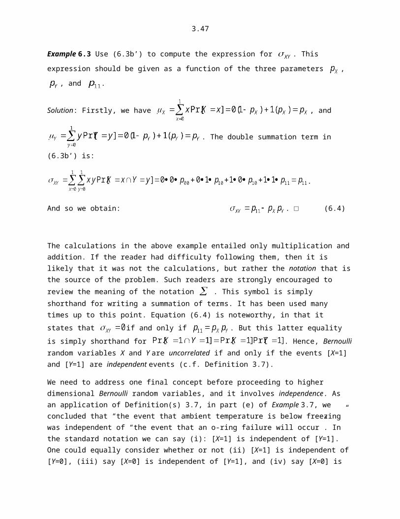
3.47

But suppose we were considering conducting an experiment where only 100 measurements were being considered. Well, if we run the above code for this value of m, we get a sum equal to 74. Running it a second time gives a sum equal to 67. And if we run the code 500 times, we could plot a histogram of the sum data, to get a better idea of the amount of uncertainty of the p-value estimator for m=100. Her is the Matlab code that allows us to conduct this investigation of how good an estimate of the true p-value we can expect:

p=0.7;m=500; % Number of simulationsn=100; % Number of subjects in any simulationu=rand(n,m);u=u-(1-p);x=ceil(u);phat=mean(x);hist(phat)

0.55 0.6 0.65 0.7 0.75 0.8 0.85 0.90

20

40

60

80

100

120

Figure 8.1 Histogram of the p-value estimator (2.7) associated with m=100 subjects, using 500 simulations.

Notice that the histogram is reasonably well centered about the true p-value of 0.7. Based on the 500 estimates of (8.1) for n=100, the sample mean and standard deviation of the estimator (8.1) are 0.7001 and 0.0442, respectively. Were we to use a 2-σ reporting error for our estimate of (8.1) for m=100, it would be ~±0.09 (or 9%).

3.48

To get an idea of how the reporting error may be influenced by the number of chosen subjects, n, used in (8.1), we embedded the above code in an n-DO LOOP, for values of n=100, 1000, and 10,000. For each value of n we computed the sample standard deviation for n=500 simulations. The code and results are given below.

>> %PROGRAM NAME: phatstd

n=[100 1000 10000];phatstdvec=[];p=0.7;m=500;for i=1:3u=rand(n(i),m);u=u-(1-p);x=ceil(u);phat=mean(x);phatstd=std(phat);phatstdvec=[phatstdvec phatstd];endphatstdvec

phatstdvec = 0.0469 0.0140 0.0046

Closer examination of these 3 numbers associated with the chosen 3 values of m, would reveal that the standard deviation of (8.1) appears to be inversely proportional to . This discovery, along with the discovery that for large enough sample size, n, the estimator has a bell-shaped pdf, is essentially the basis for:

The Central Limit Theorem for - Let be an ordered n-tuple of iid Ber(pX) random

variables. Then for sufficiently large n, the estimator has mean equal to , variance equal to

and has a pdf that is approximately normal (or Gaussian, or bell-shaped).

3.9 THE CASE OF LOCALLY CORRELATED BERNOULLI RANDOM VARIABLES

In this section we demonstrate the power of knowledge of the conditional PDF of a 2-D Bernoulli random variable, in relation to a process that is a time-indexed collection of random variables. In general, such a process is known as a random process:

3.49

Definition 9.1 A time-indexed collection of random variables, is known as a random process. If

the joint PDF of any subset does not depend on t, for any n, then the process is said to be a stationary random process.

The universe is rife with time-dependent variables that take on only one of two possible values. Consider just a few such processes from a wide range of settings:

Whether a person is breathing normally or not. Whether a drop in air temperature causes a chemical phase change or not. Whether farmers will get more that 2 inches of rain in July or not. Whether your cell phone receives a correct bit of information or not. Whether a cooling pump performs as designed or not. Whether you get married in any given year or not. Whether a black hole exists in a sector of the galaxy or not.

All of these examples are time-dependent. In the following example we address what might be termed a Bernoulli or a binary random process.

Example 9.1 Samples of a mixing process are taken once every hour. If the chemical composition is not within required limits, a value of one is entered into the data log. Otherwise, a value of zero is entered. Figure 7 below shows two randomly selected 200-hout segments of the data log for a process that is deemed to be pretty much under control.

From these data, we see that, for the most part, the process is in control. However, when it goes out of control, there seems to be a tendency to remain out of control for more than one hour.

(a) Under federal regulations, the mixture associated with an out-of-control period must be discarded. Management would like to have a computer model for simulating this control data log. It should be a random model that captures key information, such as the mean and standard deviation of a simulated data log. Pursue the design of such a model.

Well, having had Professor Sherman’s STAT 305 or 447 course, you immediately recall the notion of a Bernoulli random variable. And so, your first thought is to define the events [X=0] and [X=1] to correspond to “in” and “out of” control, respectively. To estimate the p-value for X, you add up all the ‘ones’ in the lower segment given in Figure 9.1 below, and divide this number by 200. This yields the p-value, p=12/200=0.06. You then proceed to simulate a data log segment by using the following Matlab commands:

3.50

>> u = rand(1,200);>> u= u – 0.94;>> y = ceil(u);>> stem(y)

The stem plot is shown in Figure 9.2 below.

0 20 40 60 80 100 120 140 160 180 2000

0.1

0.2

0.3

0.4

0.5

0.6

0.7

0.8

0.9

1

Time

y(t)

Time Series for Process Control State

0 20 40 60 80 100 120 140 160 180 2000

0.1

0.2

0.3

0.4

0.5

0.6

0.7

0.8

0.9

1

Time

y(t)

Time Series for Process Control State

Figure 9.1 Two 200-hour segments of the control data log for a mixing process.

Even though Figure 9.2 has general similarities to the plots in Figure 9.1, it lacks the “grouping” tendency of the ‘ones’. Hence, management feels the model is inadequate.

3.51

0 20 40 60 80 100 120 140 160 180 2000

0.1

0.2

0.3

0.4

0.5

0.6

0.7

0.8

0.9

1Simulation of Process Data Log Using a Ber(0.06) random variable

Con

trol S

tate

Time

Figure 9.2 Simulation of a data log 200-hour segment using a Ber(0.6) random variable.

(b) Use the concept of a 2-D Bernoulli random variable whose components are not assumed to be statistically independent, as the basis for your model. Specifically, X1 is the process control state at any time, t, and X2 is the state at time t+1.

To this end, you need configure the data to correspond to . You do this in the following way: For simplicity, consider the following measurements associated with a 10-hour segment: [0 0 0 1 0 0 0 0 10]. This array represents 10 measurements of X1. Now, for each measurement of then

measurement that follows it is the corresponding measurement of . Since you have no

measurement following the 10th measurement of , this means that you have only 9 measurements

of ; namely

0 0 0 1 0 0 0 0 1 0 0 1 0 0 0 0 1 0

Of these 9 ordered pairs, you have 5 (0,0) elements. And so, your estimate for would be 5/9.

Using this procedure on the second data set in Figure 9.1, you arrive at the following numerical estimates: and . It follows that .

Since , your first measurement of your 200-hour simulation is that of a Ber(0.06) random variable. You simulate a numerical value for this variable in exactly the way you did in part (a). If the number is 0, your p-value for simulating the second number is obtained using (6.2a), and if your first number was a 1, then you use a p-value given by (6.2b). Specifically,

3.52

.

The Matlab code for this simulation is shown below.

%PROGRAM NAME: berprocess.m% This program generates a realization% of a Ber(p00, p10, p01,p11) correlated processnpts = 200;y=zeros(npts+1,1); % Stationary Joint Probabilities between Y(k) and Y(k-1)p01=0.05;p10=p01;p11=0.05p00 = 1 - (p11 + p10 + p01);pvec = [p00 p10 p01 p11]%Marginal p for any Y(k)p=p11 + p10% -------------------------x = rand(npts+1,1);y(1)= ceil(x(1)- (1-p)); % Initial conditionfor k = 2:npts+1 if y(k-1)== 0 pk = p10/(p00 + p10); y(k)=ceil(x(k) - (1-pk)); else pk = p11/(p11 + p10); y(k)=ceil(x(k) - (1-pk)); endendstem(y(1:200))xlabel('Time')ylabel('y(t)')title('Time Series for Process Control State')

Running this code twice, gives the simulation segments in Figure 3.9 below.

3.53

0 50 100 150 200 2500

0.1

0.2

0.3

0.4

0.5

0.6

0.7

0.8

0.9

1

Time

y(t)

Time Series for Process Control State

0 50 100 150 200 2500

0.1

0.2

0.3

0.4

0.5

0.6

0.7

0.8

0.9

1

Time

y(t)

Time Series for Process Control State

Figure 9.3 Two 200-hour data log simulations using a 2-D Bernoulli random variable with probabilities , , and hence, .

Management feels that this model captures the grouping tendency of the ones, and so your model is approved. Congratulations!!!

Before we leave this example, let’s think about the reasonableness of the ‘ones’ grouping tendency. What this says is that when the process does go out of control, it has a tendency to remain out of control for more than one hour. In fact, the above conditional probability states that if it is out of control during one hour, then there is an 83% chance that it will remain out of control the next hour. This can point to a number of possible sources responsible for the process going out of control. Specifically, if the time constant associated with either transient nonhomogeneities in the chemicals, or with a partially blocked mixing valve is on the order of an hour, then one might have reason to investigate these sources. If either of these sources has a time constant on the order of hours, then the above model can be used for early detection of the source. Specifically, we can use a sliding window to collect overlapping data

3.54

segments, and estimate the probabilities associated with . If a blockage in the mixing valve takes hours to dissolve, then one might expect the above probability value 0.8333 to increase. We can use this logic to construct a hypothesis test for determining whether we think the valve is blocked or not. We will discuss hypothesis testing presently. Perhaps this commentary will help to motivate the reader to look forward to that topic.

PROBLEMS

PROBLEM 1 Consider a military carrier that has 5 critical parts. Define the random variables where the event corresponds to the event that “the ith part fails”, and the event corresponds to the event that the ith part does NOT fail. Then, clearly, the random

variable corresponds to the number of failed parts. The goal of this problem is to arrive

at the probability density function (pdf) for Y, as a function of assumed pdfs for the random

variables . Let .

(a) In this part, we will assume the following assumptions hold:

(A1): The components of are mutually independent.

(A2): The parameters are all the same value (i.e. p).

Here, we will assume that p = 0.05. These assumptions imply that Y has a Binomial(p=0.05, n=5) pdf. Plot this pdf, and compute and . Show the details of your computations.

(b) Even though the assumption (A2) is mathematically convenient, in this situation it is entirely unreasonable! Explain.

(c) In order to arrive at a more realistic probability model for Y, notice that each component of the 5-D random variable is a “zero/one” random variable; that is, , where . Give a clear mathematical description of the sample space for . Also, state the number of elements in this space.

(d) It should be obvious that the sample space for is . For each of the

following elemental subsets of SY, describe the corresponding subset of AND give the number of elements in that subset.

{0}: ; N0 = 1{1}: ; N1=5

{2}: ; N2=

3.55

{3}: ; N2=

{4}: ; N2=

{5}: ; N5 = 1

(e) We are now in a position to address the probabilities associated with the subsets in (d). We have relaxed the assumption (A2), but for now, we will retain assumption (A1). In this case, we have

(1)

Suppose that the failure probabilities of the parts are: p1=0.1 ; p2=0.02 ; p3= 0.01 ; p4= 0.07 and p5 = 0.05. Notice that the average of these probabilities is 0.05, which was the value of p assumed in (a). Using the first two subsets and (1), compute the probability that no more than one part fails. Then comment on how this number compares to the same probability under the assumption that (A2) holds.

PROBLEM 2 Define the random variable, X =”the act of recording whether a crack is detected in any specified region along an aircraft wing”; specifically, [X=1] denotes the event that a crack was detected. The following 5 rows of data correspond to crack information associated with 5 wings. A total of 20 regions were scanned for each wing.

x1 = [0 0 0 0 1 0 0 0 1 1 1 0 0 0 0 1 1 0 0 0];x2 = [1 1 0 0 0 0 0 0 1 1 0 0 0 0 0 0 0 1 1 1];x3 = [0 0 0 1 0 0 0 1 1 1 0 0 0 0 0 1 1 1 0 0];x4 = [0 1 0 0 0 0 0 0 0 1 1 0 0 0 0 1 0 0 0 1];x5 = [0 1 0 1 1 0 0 0 0 1 1 1 0 0 0 0 0 1 1 0];

(a) View these 100 numbers as measurements of where, for any i,j , Xi j is a Bernoulli

random variable with p-value, pX . Give (i) the expression for the estimator, call it , (ii) the estimate associated with the above measurements, and (iii) a description, in words, of the generic random variable, X, that this study intends to address.

(b) For X defined as above, define the random variable Y = “the act of recording whether a crack is detected in the region scanned directly after the region associated with X”. Thus, for this 2-D random variable (X,Y) the above data yields a total of 19(5)=95 measurements. [i.e. you pair the second with the first, the third with the second, the fourth with the third, …, the 20th with the 19th for each wing.] Use

3.56

these measurements to estimate Pr[Y=1 | X=1]. Noting that IF X and Y were independent, then we would have Pr[Y=1 | X=1] = Pr[Y=1] ( = Pr[X=1] ) since, marginally, X and Y have exactly the same probability model), then, if your computed conditional probability is close to your answer in (a), you would suspect that X and Y are independent. Based on your numerical answers in (a) and for the conditional probability, what would you conclude? Is your conclusion supported by a visual inspection of the data? Explain.

(c) Use your answers to (a) and (b) in order to make a decision as to whether you feel that X and Y are independent.

PROBLEM 3

(a) ”In a certain community, 8% of adults over age 50 have diabetes.” Translate this into a statement about a Bernoulli random variable, X.

(b) ”The health service correctly diagnoses 95% of those who have diabetes.” Translate this into a conditional probability statement in relation to a second Bernoulli random variable, Y, given that X equals an appropriate value.

(c) ”Of those who do not have diabetes, 2% are diagnosed as having it.” Translate this into a conditional probability statement in relation to a second Bernoulli random variable, Y, given that X equals an appropriate value.

(d) Find the values of the 4 probabilities associated with the 2-d Bernoulli random variable (X,Y). Then compute the marginal probabilities for X and Y.

(e) ”Find the probability that an adult over 50 will be diagnosed as having diabetes.” To this end, first identify the subset of the sample space for (X,Y) for which the probability is to be found. Then use the results in (c) to compute the probability.

(f) ”Given that a man diagnosed as having diabetes, compute the probability that he actually has it.”

PROBLEM 4 The purpose of this problem is to investigate how the p-value of a Bernoulli(p) random variable influences how well the Normal PDF approximation is for the sample mean, of

. Recall that the sum, Y, of n iid Ber(p) random variables is Binomial(n,p) with

3.57

mean np and with variance np(1-p). Hence, has mean p and variance p(1-p)/n. Furthermore, it has exactly the same Binomial pdf as Y, but on the set {0, 1/n, 2/n,…,1} as opposed to {0,1,2,…,n}. For each of the following cases, overlay plots of the true pdf for and the normal approximation to it. Finally, discuss how accurate the normal approximation is, as a function of n and p. In particular, comment on whether the “rule of thumb” on p.218 seems to be valid. (a) n=30 and p=0.5 ; (b) n=30 and p=0.05 ; (c) n=100 and p=0.5 ; (d) n=100 and p=0.05

PROBLEM 5. The main purpose of this problem is to take advantage of the results obtained in PROBLEM 4. Recall that in that problem we addressed the probability structure of the estimator or the

parameter , corresponding to the Bernoulli random variable, X. For the n-tuple of data

collection random variables where we assume that are iid (i.e. the

components of are identically distributed with the distribution of X, and that they are mutually independent). Then the estimator

is a scaled Binomial random variable; that is, it has the probability expression for a

Binomial random variable, but over the scaled sample space . The mean and variance

of this estimator are and , respectively. We will consider the application of this

estimator to quality assurance.

(a) Suppose that our supplier of DC power supplies used in our laptop computers rates the model we use at 9 volts, with a uncertainty of volts. Let V denote the act of measuring the voltage of any chosen power supply, and suppose that V has a normal (i.e. bell-shape) pdf. Using the above rating information, give the numerical values of the mean and standard deviation for V:

(b) Use the Matlab command normpdf to obtain a plot of the pdf . The horizontal axis of your plot

should include the interval . Label the axes of your plot and include a title.

(c)We know that if the supply voltage is less than 8.5 volts, the video card will be very likely to not function properly. On your plot in (b): (i) highlight the event that, in the standard notation, is , (ii) shade the area beneath the curve associated with this event. (This area is a visual representation of

.), and (iii) use the Matlab command normcdf to obtain a numerical value for this area. Let this value be denoted as p.

(d) At the receiving dock, prior to signing off on a shipment of power supplies, we currently inspect 25 randomly selected power supplies. For the kth power supply identify the event with the event

. Then is a 25-tuple random variable, whose components are iid Bernoulli(p) random variables. Compute the numerical values of the mean and standard

deviation of .

3.58

(e) Use your answers to (d) to compute the uncertainty range for the estimator, . Then comment on how why this interval is problematic.

(f) It should be clear from (c) that it makes no sense to use the ‘rule’: If falls outside of the region , then the shipment should be rejected. And so, we need to go ‘back to basics’.

Clearly, we will not reject the shipment in the event that =0, which is [ =0]. Our rule of rejection will be an event of the form , where the numerical value of the threshold needs to be specified . It

only makes sense that the numerical value of should be one of the elements of the sample space for ,

which is . Suppose that we choose ; that is, if two or more tested power supplies have voltages less than 8.5 volts, we will reject the shipment. Compute the probability that we will reject a shipment.

(g) Based on your answer in (f), over the course of 100 shipments, approximately how many should we expect will be rejected?

(h) Suppose that of the most recent 100 shipments, we have rejected two. Assuming that acceptance/rejection of any shipment is independent of acceptance/rejection of any other shipment. Compute the probability that we will reject two or more of 100 shipments. Then, discuss whether or not we should consider challenging the supplier on his claimed voltage mean and standard deviation numbers.

(i) The decision we arrived at in (h) did not consider which two of the last 100 shipments were rejected. Suppose that, in reviewing the receiving log, we found that we, in fact, rejected two of the past 10 shipments. Repeat part (h) for this situation.

(j) Suppose we have an agreement with the supplier that, beginning at the date at which a shipment is rejected, should any of the next 51 shipments be rejected, the supplier will give us a 25% rebate of our total purchases during that period. Find the probability that we will get a rebate.

PROBLEM 6. In PROBLEM 5(e) you should have found that the sample size, n, was simply too small to assign meaning to the uncertainty range for the estimator, . Use tools developed in Homework 4 to determine a suitable value of n, so that it is meaningful. It should be noted that the more power supplies that are tested, the more expensive that task becomes. Hence, you should try to find as small a value for n as you feel is necessary.

PROBLEM 7. Suppose it is desired to recruit 20 of the local population to serve on the community security force. From historical data, it is known that one of every eight recruits will desert the force within the first month of being recruited. In this problem we will assume that the desertion of one person in no way influences whether any other person will desert. Determine the smallest number, call it n, of locals that need to be recruited if we require that the probability of having at least 20 members remain after the first month is at least 0.9.

3.59

PROBLEM 8. During the Spring months for a given country, historical data has shown that significant rainfalll occurs on an average of one in every five days. Suppose that the season lasts for 60 days.

(a) Use the Matlab command rand.m to construct a code that can simulate a 60-day data record of no-rain/rain events, assuming that whether or not it rains on any given day is independent of whether or not it rains on the next day. Verify your code by running and plotting results of two simulations. From each one, estimate the p-value for X=the act of noting whether it does not (0) or does (1) rain on any given day.

(b) Run 10,000 simulations in order to investigate the probability structure of the estimator of p. Your investigation should address (i) the mean , (ii) the standard deviation, and (iii) the pdf shape of .

(c) Repeat parts (a) and (b) in the situation where the independence assumption in (a) is not supported by historical data. Specifically, suppose that the data supports the conditional probability , where

for any chosen k. Comment on how your results compare to those of (a)

and (b).