Holographic strain analysis: extension of fringe-vectormethod to include perspective

R. Pryputniewicz and Karl A. Stetson

A method has been published recently that permits determination of complete strain and rotation tensorsof homogeneously deformed objects directly from fringes that are observed on their surfaces. However,the illumination and observation directions had to be considered constant over the regions of interest toapply the technique. This paper presents an extension of that theory to include both observation and illu-mination perspectives. It is shown that bulk translations of an object combine with linear variations in thedirections of observation and illumination to generate fringe vectors that add directly to those generatedby the object's homogeneous transformations. These linear variations are calculable from illuminationand observation geometry.

Introduction

A current problem of considerable interest in thefield of hologram interferometry is that of extractingobject strain from fringes observable in hologram re-constructions. One method, 1 which may be calledthe fringe-vector method of holographic strain analy-sis, provides a method of obtaining homogeneousstrains and rotations directly from fringe spacings onthree-dimensional objects. The method utilizes thefact that such object motions yield fringes that ap-pear like equidistant laminae intersecting the surfaceof the object. It is possible to represent these lami-nae by a fringe vector whose scalar product with thespace vector yields the fringe-locus function andwhich, in turn, can be related to the sensitivity vectorby that matrix transformation that describes homo-geneous strain and rotation.

The primary source of difficulty in applying thismethod of holographic strain analysis is that it pre-sumes that the sensitivity vector is constant in mag-nitude and direction over the region of interest.This is rarely, if ever, true, and the fact that errorscan occur by making this approximation in practicehas been highlighted recently by Dandliker et al. 2

We shall, in this paper, present a method of correct-ing for the errors introduced by variations of the sen-sitivity vector, so that the fringe-vector method canbe used even in the presence of perspective. The

R. Pryputniewicz is with the University of Connecticut, Depart-ment of Mechanical Engineering, Storrs, Connecticut 06268; K. A.Stetson is with United Technologies Research Center, Instrumen-tation Laboratory, East Hartford, Connecticut 06108.

Received 19 August 1975.

error takes the form of a vector that must be sub-tracted from the experimentally determined fringevector before it is related to the sensitivity vector bythe strain and rotation matrix. We shall also includean improved method for experimentally determiningthe fringe vectors.

Fringe Vectors Due to Perspective

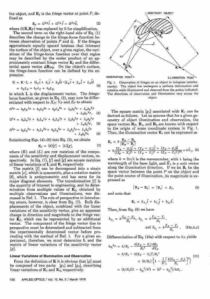
A fringe-locus function , constant values of whichdefine fringe loci on an object surface, depends on thesensitivity vector and the space vector that definesthe coordinates of the object surface. If the illumi-nation and observation vectors are K1 and K2, asshown in Fig. 1, we may define the sensitivity vectorK = K2 - K1 , from which = K-L, where L is thevector displacement of an object point. Let us as-sume that the value of this fringe-locus function at apoint P on the object Q(K,Rp) is known, where Rp isthe space vector from the origin of some coordinatesystem to point P. Then, the fringe-locus functionat a nearby point Q on the object Q(K,RQ) may beexpressed in terms of Q(K,Rp) by means of a Taylorseries expansion

Q(K,RQ) = S2(K,R + ARpQ)

= S2(K,Rp) + AXPQS2XP + YPQ YP+ AZPQE2ZP

= E2K,Rp) + (AXPQz + AYPQ + AZPQk) (1)

.(O + 2YJ+ QZPk

= 2(K,Rp) + ARpQ Kf,

where QXp, QYP, QZP denote differentiations with re-spect to Xp, Yp, and Zp, respectively. In Eq. (1),ARpQ is the space vector from point P to point Q on

March 1976 / Vol. 15, No. 3 / APPLIED OPTICS 725

the object, and Kf is the fringe vector at point P, dfined as

K/ = Xp + yp + RzPpwhere Q(K,Rp) was replaced by Q for simplification

The second term on the right-hand side of Eq. describes the change in the fringe-locus function tween observation of points P and Q. If the fringapproximate equally spaced laminae that intersEthe surface of the object, over a given region, the vaations of the fringe-locus function over that regimay be described by the scalar product of an aproximately constant fringe vector Kf and the diffEential space vector ARpQ. On the object's surfa(the fringe-locus function can be defined by the epression

E = K- L = (kXi + kyj + kzk) * (Li + Ly + Lk)

= kLx + kyLy + kzLz,in which L is the displacement vector. The fringlocus function, as given in Eq. (3), may now be diffEentiated with respect to Xp; Yp and Zp to obtain

QXp = kLxx + kLyxP + kzLzXP + LxkxXP + Lyky P+ LzkzXP,

QYP = kzxLxy + kyLYYP + kzLzYP + LkxYP + LykyyP+ LkzyP,

QZP = kLxzP + kLZP+ kzLzZ + LXzP + LykYZP+ LzkzZP.

Substituting Eqs. (4)-(6) into Eq. (2), we obtain

Kf = (K)[f] + (L)[g],

.e-

(2)

(1)ie-gesectri-onUp

)r-ce,ex-

(3)

ge-er-

(4)

(5)

(6)

(7)

where (K) and (L) are row matrices of the compo-nents of the sensitivity and displacement vectors, re-spectively. In Eq. (7), [f] and [g] are square matricesof linear variations of L and K, respectively.

The matrix Vf] can be decomposed into a strainmatrix [e], which is symmetric, plus a rotation matrix[0], which is antisymmetric and has zeros for itsmajor diagonal elements. The transformation [/] isthe quantity of interest in engineering, and its deter-mination from multiple values of Kf, obtained bymultiple observations and illuminations, was dis-cussed in Ref. 1. The role of perspective in introduc-ing errors, however, is clear from Eq. (7). Bulk dis-placements of the object, combined with the linearvariations of the sensitivity vector, give an apparentchange in direction and magnitude to the fringe vec-tor Kf, which can be represented by an additionalvector. The component of the fringe vector due toperspective must be determined and subtracted fromthe experimentally determined vector before pro-ceeding with the method of Ref. 1. For a given ex-periment, therefore, we must determine L and thematrix of linear variations of the sensitivity vector[g]-

Linear Variations of Illumination and Observation

From the definition of K it is obvious that [g] mustbe composed of two parts: [g1 ] and [g 2], describinglinear variations of K1 and K2, respectively.

Fig. 1. Observation of fringes on an object in hologram interfer-ometry. The object has undergone a uniform deformation aridrotation while illuminated and observed from the points indicated.The directions of observation and illumination vary across the

object.

The square matrix [gi] associated with K1 can bederived as follows. Let us assume that for a given ge-ometry of object illumination and observation, thespace vectors Rp, R1, and R2 are known with respectto the origin of some coordinate system in Fig. 1.Then, the illumination vector K1 can be expressed as

K = k R -R

k (p - 1) + (YP '. Y1) + (Zp - ZI =kk, (8)L(X _ X) 2 + ( - y )2 + (z - zX1Y/ =

where k = 27r/X is the wavenumber, with X being thewavelength of the laser light, and K1 is a unit vectoralong the illumination direction. If we let Ri be thespace vector between the point P on the object andthe point source of illumination, its magnitude is ex-pressed as

JRP-RI = Ri = Ri,

and note that

K = k I + ky1 + kk.

Then, from Eq. (8) we have

h = k, P 1, ky = k YP = -

and kZ = kP-Z

(9)

(l0a,b,c)

Differentiation of Eq. (lOa) with respect to Xp yields

kx xP = k/R 1 _ k(X- x 1 ) dR

= k/Ri - k(X1p - XRi3 (11)

= (k/Ri) {1 1[k(Xp-X).

= (k/R)(I - kx12/k2) = (k2 - k., 2)/kRi.

726 APPLIED OPTICS / Vol. 15, No. 3 / March 1976

The magnitude of K1 may be expressed as

IK, = k = (kx12 + k 2 + kZ1 2)W/.

Using Eq. (12) we obtain from Eq. (11)

k,,XP = (k 2 + kZ2)IkRi . (13)

Differentiating Eq. (lOa) again, but now with respectto Yp, we obtain

kXPY = -k(Xp - Xl)(Yp - Y)/Ri 3

= -(1/kR)[k(Xp - X 1)/RJ[k(Y - Yr)/R] (14)

= -k_,k,,/kRi.

Following the procedure outlined above, the remain-ing derivatives of components of the illuminationvector may be obtained, and, finally, the matrix oflinear variations of K1 can be expressed as

(ky12 +

[gi = (kRi) -kyk.

-k klIk

-k,.ky -k-i~k 2 + k 1

2 ) -k k .

-k 1lky1 (kXi2 + k2) j

In a similar manner, the matrix of linear variations ofK2 can be evaluated as

kz22)(ky2 2 +

[g 2] = (/kR,) -k k

k 2 kX2

-kx 2 kY2 -kx 2 kZ2

(kX22 + k, 22) -k Y2kZ2 I

-k 2 kY2 (k, 22 + ky22)j

where Ro = I Rol = I R2-Rpl is the magnitude of thespace vector from point P to the point of observation.Note, however, that Ro and Ri must be given signs toaccount for the divergence and convergence of the il-lumination and observation perspectives. R or Riwill be positive if directed outward and negative if in-ward. The matrix of linear variations of K is ob-tained simply by subtraction of the matrices given inEqs. (15) and (16), viz.,

[g] = [g2] - [g1 ]. (17)

Finally, the corrected fringe vector (K) [f] for illu-mination and observation perspective can be ob-tained from Eq. (7) as

(K)[f] = Kf - (L)[g], (18)

(12)

The fringe-locus function Q may be defined by theequation

0m(KRp) = KF Rpm + N (19)

in which Kf is the fringe vector;

Rpm

is the space vector from the origin of an arbitrarycoordinate system to point Pm on the object in Fig. 1,and N is the number of fringes (value of ) thatwould have been seen had the zero-order fringe beenidentifiable. Obviously, no matter how carefully theobservations are made, there will always be someerror inherent in the measurements. Thus Eq. (19)should be written as

Em = (Kf Rp + N) - Rm S (20)

where Em denotes the error between the actual andmeasured values of the fringe-locus function at themth point on the object. Ideally, a set of four linearsimultaneous equations of the type of Eq. (19) wouldbe sufficient to determine N and the Cartesian com-ponents kfx, kfy, and kfz of Kf. However, the valueof the determinant of these equations may be smallbecause of the limited size of the hologram plate (ifthe solid angles the hologram subtends at the objectis small), and hence large errors may be expected.Alternatively we may generate an overdetermined setof linear simultaneous equations relating the fringe-locus function to the four unknowns and obtain theresult by the least-squares theory.

Let us assume that we are able to observe r pointsin a holographic image of a given object, and that it ispossible to determine Rp and for each of thesepoints by fringe intersections. As a result, we obtainr expressions of the type of Eq. (20), one for eachpoint on the object. The goal of the analysis is to ad-just the coefficients in this system of equations insuch a way as to minimize the summation of all theerrors squared, that is,

r rZE 2 = Z (kXp + kYY + kfzZ +-I1 M=1 m z

N - Qm)2(21)

by letting

Kf = ki + kj + kkwhere Kf may be otained using the method proposedin Ref. 1, and L can be calculated using, for example,least-square techniques.3

Determination of Fringe Vectors

Although the method given in Ref. 1 for calculatingthe fringe vector from experimental data is adequatefor many situations, it does not yield the fringe vectorthat best fits all the data points available for compu-tation. The best fit for the fringe vector is found byapplying least-squares error theory as follows:

and

Rpm - Xp + Yp + Zpmi?.

If

EZEm2m1

is minimum, the partial derivative of Eq. (21) withrespect to kfx, fy, kfz, and N must be zero, whichresults in the following:

March 1976 / Vol. 15, No. 3 / APPLIED OPTICS 727

kZi 2)

r r,(kiXXp + kfmYP + k fzZ, + N)X = m1Xp;

r rE(kXXpm + kyYPm + kfzZm + N)YPm = m ;

r ~~~~~~~~~~~~~~rE (kfXp + kYpm + kfzZp + N)ZPm, = Z umZPm;

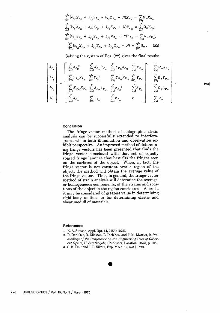
r r

E (k jp. + kfyYpm + kzZPm + N) = Z12m (22)

Solving the system of Eqs. (22) gives the final result:

7X 2 Z1 XP YPM -I -1 MXP.

myX E] ZXPZP E1 XPm m

kfz = 2 r r (23)N _ Z pmXPm Z=Pm p ZpZPm r Zmkfz M=J m=1 m=I m m=1 =

r rLl ZZ r ~

Conclusion

The fringe-vector method of holographic strainanalysis can be successfully extended to interfero-grams where both illumination and observation ex-hibit perspective. An improved method of determin-ing fringe vectors has been presented that finds thefringe vector associated with that set of equallyspaced fringe laminae that best fits the fringes seenon the surfaces of the object. When, in fact, thefringe vector is not constant over a region of theobject, the method will obtain the average value ofthe fringe vector. Thus, in general, the fringe-vectormethod of strain analysis will determine the average,or homogeneous components, of the strains and rota-tions of the object in the region considered. As such,it may be considered of greatest value in determiningrigid-body motions or for determining elastic andshear moduli of materials.

References1. K. A. Stetson, Appl. Opt. 14, 2256 (1975).2. R. Dinliker, B. Eliasson, B. Ineichen, and F. M. Mottier, in Pro-

ceedings of the Conference on the Engineering Uses of Coher-ent Optics, U. Strathclyde, (Publisher, Location, 1975), p. 125.

3. S. K. Dhir and J. P. Sikora, Exp. Mech. 12, 323 (1972).

0

728 APPLIED OPTICS / Vol. 15, No. 3 / March 1976