Holographic models of inflation - University of Miami · Holographic universe At the end of this period we arrive at a FRW spacetime and small inhomogeneities with super-horizon correlations

Holographic modelsof inflation

Kostas SkenderisInstitute for Theoretical Physics,Gravitation and AstroParticle PhysicsAmsterdam (GRAPPA),KdV Institute for MathematicsUniversity of Amsterdam

Kostas Skenderis Holographic models of inflation

References

The talk is based onA. Bzowski, P. McFadden, KS, Holographic predictions forcosmological 3-point functions, arXiv:1112.1967P. McFadden, KS, Cosmological 3-point correlators fromholography, arXiv:1104.3894R. Easther, R. Flauger, P. McFadden, KS, Constraining holographicinflation with WMAP, arXiv:1104.2040.

Earlier work with Paul McFaddenHolography for Cosmology, arXiv:0907.5542The Holographic Universe, arXiv:1007.2007Observational signatures of holographic models of inflation,arXiv:1010.0244Holographic Non-Gaussianity, arXiv:1011.0452

Related workJ. Maldacena, G. Pimentel, On graviton non-Gaussianities duringinflation, arXiv:1104.2846


Introduction

Any gravitational theory should be holographic, i.e. it should havea description in terms of a non-gravitational theory in onedimension less.There is no holographic construction that works in general todate; explicit examples depend on the form of asymptotics.The properties of the dual theory depend also on theasymptotics.

The best-understood examples originate from string theory viadecoupling limits of branes:D3, M5 etc. branes→ asymptotically AdS spacetimes→ local QFTthat in the UV becomes conformal.D2, D4 etc. → asymptotically power-law spacetimes→ local QFTwith a generalized conformal structure.


Holographic inflation

Here I will describe a holographic framework for inflationaryspacetimes that:

1 approach de Sitter spacetime at late times,

ds2 → ds2 = −dt2 + e2tdxidxi, as t →∞

2 approach power-law scaling solutions at late times ,

ds2 → ds2 = −dt2 + t2ndxidxi, (n > 1) as t →∞

These backgrounds have the property that they are in 1-1correspondence with backgrounds that describe holographic RGflows, either asymptotically AdS or asymptotically power-law.


Holographic universe

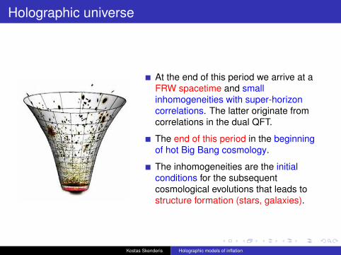
At the end of this period we arrive at aFRW spacetime and smallinhomogeneities with super-horizoncorrelations. The latter originate fromcorrelations in the dual QFT.

The end of this period in the beginningof hot Big Bang cosmology.

The inhomogeneities are the initialconditions for the subsequentcosmological evolutions that leads tostructure formation (stars, galaxies).


Domain-wall cosmology correspondence

The correspondence between inflationary spacetimes andholographic RG flows is a special case of a more generalDomain-wall/Cosmology correspondence (DW/C) [KS, Townsend(2006)] and can be understood as analytic continuation.For holographic RG flows, there is a well-established holographicdictionary.One may express the analytic continuation associated with DW/Cin QFT terms: one analytically continues the momenta q and therank of the gauge group N:

q → q̄ = −iq, N → N̄ = −iN


Holographic framework [McFadden, KS (2009)]


Weakly coupled gravity

To test this framework we analyzed the case where gravity is weaklycoupled, so standard treatments are available.

We worked out the cosmological 2- and 3-point functions ofscalar and tensor perturbations around a general single scalarinflationary background.We worked out the 2- and 3-point functions of the stress energytensor of the corresponding domain-wall background, usingstandard gauge/gravity duality.We found that the cosmological correlators can beexpressed in terms of the QFT correlation functions atstrong coupling upon analytic continuation.

⇒ Standard inflation is holographic.


Holographic formulae: preliminaries

The 2-point function of Tij in a flat spacetime has the form

〈Tij(q̄)Tkl(−q̄)〉 = A(q̄)Πijkl + B(q̄)πijπkl,

where Πijkl = 12 (πikπlj + πilπkj − πijπkl), πij = δij − q̄iq̄j/q̄2.

We found useful to use a helicity basis.

Tij → T,T(s), s = ±1

where T is the trace of Tij and the transverse traceless part of Tij

is traded for T±.In cosmology, the physical degrees of freedom are a scalarmode, ζ, and transverse traceless tensor modes γ̂ij. In a helicitybasis:

(δφ, hij) → ζ, γ̂(s), s = ±1


Holographic formulae: 2-point functions

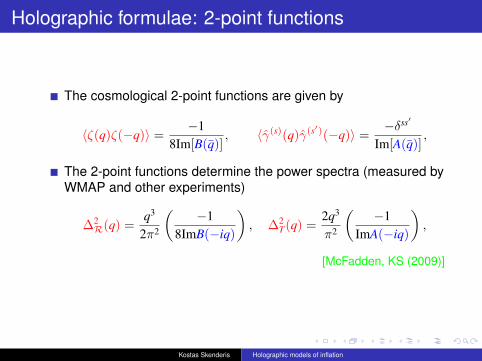
The cosmological 2-point functions are given by

〈ζ(q)ζ(−q)〉 =−1

8Im[B(q̄)], 〈γ̂(s)(q)γ̂(s′)(−q)〉 =

−δss′

Im[A(q̄)],

The 2-point functions determine the power spectra (measured byWMAP and other experiments)

∆2R(q) =

q3

2π2

(−1

8ImB(−iq)

), ∆2

T(q) =2q3

π2

(−1

ImA(−iq)

),

[McFadden, KS (2009)]



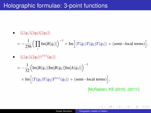
• 〈ζ(q1)ζ(q2)ζ(q3)〉

= − 1256

( ∏i

Im[B(q̄i)])−1

× Im[〈T(q̄1)T(q̄2)T(q̄3)〉+ (semi−local terms)

],

• 〈ζ(q1)ζ(q2)γ̂(s3)(q3)〉

= − 132

(Im[B(q̄1)]Im[B(q̄2)]Im[A(q̄3)]

)−1

× Im[〈T(q̄1)T(q̄2)T(s3)(q̄3)〉+ (semi−local terms)

],

[McFadden, KS (2010), (2011)]



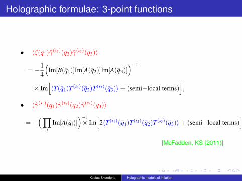
• 〈ζ(q1)γ̂(s2)(q2)γ̂(s3)(q3)〉

= −14

(Im[B(q̄1)]Im[A(q̄2)]Im[A(q̄3)]

)−1

× Im[〈T(q̄1)T(s2)(q̄2)T(s3)(q̄3)〉+ (semi−local terms)

],

• 〈γ̂(s1)(q1)γ̂(s2)(q2)γ̂(s3)(q3)〉

= −( ∏

i

Im[A(q̄i)])−1× Im

[2〈T(s1)(q̄1)T(s2)(q̄2)T(s3)(q̄3)〉+ (semi−local terms)

].

[McFadden, KS (2011)]


New holographic models

While conventional inflationary models are related with stronglycoupled QFT, new models arise when we consider the QFT atweak coupling (but still at large N).In these models, the very early universe is in a non-geometricphase. This phase should have a description in string theory interms of a strongly coupled sigma model. Here we useholography to describe it.


Dual QFT

To make predictions we need to specify the dual QFT. The twoclasses of asymptotic behaviors correspond to two classes of dualQFT’s.

asymptotically de Sitter → QFT is deformation of a CFTasymptotically power-law → QFT has generalized conformalstructure

Here we discuss theories of the second type.


Dual QFT

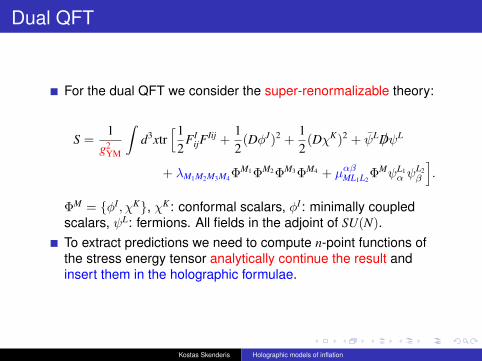
For the dual QFT we consider the super-renormalizable theory:

S =1

g2YM

∫d3xtr

[12

FIijF

Iij +12(DφJ)2 +

12(DχK)2 + ψ̄L /DψL

+ λM1M2M3M4ΦM1ΦM2ΦM3ΦM4 + µαβ

ML1L2ΦMψL1

α ψL2β

].

ΦM = {φI , χK}, χK : conformal scalars, φI : minimally coupledscalars, ψL: fermions. All fields in the adjoint of SU(N).To extract predictions we need to compute n-point functions ofthe stress energy tensor analytically continue the result andinsert them in the holographic formulae.


Holographic power spectrum

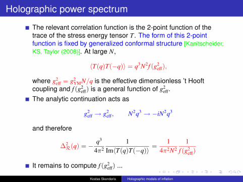
The relevant correlation function is the 2-point function of thetrace of the stress energy tensor T. The form of this 2-pointfunction is fixed by generalized conformal structure [Kanitscheider,KS, Taylor (2008)]. At large N,

〈T(q)T(−q)〉 = q3N2f (g2eff),

where g2eff = g2

YMN/q is the effective dimensionless ’t Hooftcoupling and f (g2

eff) is a general function of g2eff.

The analytic continuation acts as

g2eff → g2

eff, N2q3 → −iN2q3

and therefore

∆2R(q) = − q3

4π2

1Im〈T(q)T(−q)〉

=1

4π2N2

1f (g2

eff)

It remains to compute f (g2eff) ...



When g2eff is small, one finds that the function f (g2

eff) has the form

f (g2eff) = f0(1− f1g2

eff ln g2eff + f2g2

eff + O[g4eff]).

→ f0 is determined at 1-loop in perturbation theory. It has beencomputed in [McFadden, KS (2009)].

→ f1 is determined at 2-loop in perturbation theory. It has not beencomputed to date.

→ f2 is related with an infrared generated scale qIR ∼ g2YM

[Jackiw,Templeton (1981)][Appelquist, Pisarski(1981)]. As long as oneprobes the theory at scales large compared with the IR scale,this term is negligible.



Redefining variables, f1g2YMN = gq∗, where q∗ is a reference

scale, we obtain the final formula:

∆2R(q) = ∆2

R1

1 + (gq∗/q) ln |q/gq∗|,

→ ∆2R = 1/(4π2N2f0). Smallness of the amplitude is related with the

large N limit: matching with observations implies N ∼ 104.→ When (gq∗/q) � 1 one may rewrite the spectrum in the

power-law form

∆2R(q) = ∆2

Rqns−1, ns(q)− 1 = gq∗/q

Thus the small deviation from scale invariance appears to berelated with the coupling constant of the dual QFT being small.


Holographic model vs slow-roll inflation

This is a rather different spectrum than that of generic slow-rollmodels. In such models the dependence of ns on q is ratherweak. The "running" αs = dns/d ln q is higher order in slow-rollthan (ns − 1),

αs/(ns − 1) ∼ ε

In contrast, in the holographic model, αs ∼ (ns − 1). In fact, alldkns(q)/d ln qk are of the same order in the holographic model.Given that the power-law ΛCDM model, in which ns is a constant,fits remarkably well the WMAP and other astrophysical data, onemay wonder whether already existing data are sufficient to ruleout this class of holographic models.We thus undertook the task to make a dedicated data analysis[Easther, Flauger, McFadden, KS (2011). Related work appeared in[Dias (2011)].


Holographic model vs ΛCDM

The power-law ΛCDM model depends on six parameters. Fourdescribe the composition and expansion of the universe and theother two are the tilt ns and the amplitude ∆2

R of primordialcurvature perturbations.The holographic ΛCDM model depends on the same set ofparameters, except that the tilt ns is replaced by the parameter g.We determined the best-fit values for all parameters for bothmodels and used Bayesian evidence in order to make a modelcomparison.


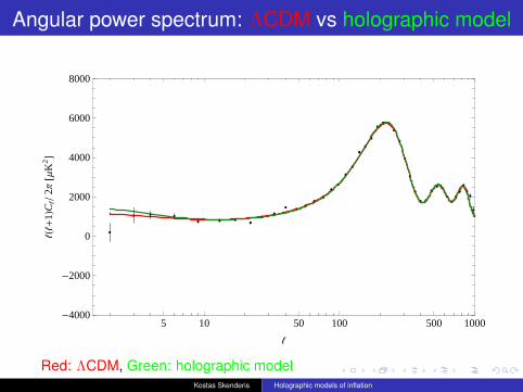
Angular power spectrum: ΛCDM vs holographic model

5 10 50 100 500 1000-4000

-2000

0

2000

4000

6000

8000

{

{H{

+1L

C{�2

Π@Μ

K2

D

Red: ΛCDM, Green: holographic modelKostas Skenderis Holographic models of inflation

Parameter estimation

The estimated values for the five common parameters of the twomodels are roughly within one standard deviation of each other.The data favor negative values of g (red spectrum) with centralvalue g = −1.27× 10−3.The holographic model is compatible with current data, but theoverall fit is somewhat better for ΛCDM.For model comparison, we would like to know the probability fora model given the data. This is computed by the Bayesianevidence E. We computed this this quantity and found the resultto be inconclusive.

More data is required to decide between the two models.


WMAP and Planck data WMAP Cosmological Parameter Plotter

Solid line:

α = −(ns−1)


Non-Gaussianities

Non-Gaussianity implies non-zero higher-point correlation functions.The lowest order is the 3-point function, or bispectrum, of curvatureperturbations ζ:

〈ζ(q1)ζ(q2)ζ(q3)〉 = (2π)3δ(∑

qi)B(qi)

Non-Gaussianity is important as it potentially provides a verystrong test of inflationary models. The amplitude of thebispectrum is parametrised by fNL:

B(qi) = fNL × (shape function)

Different inflationary models give different predictions for fNL andshape function.


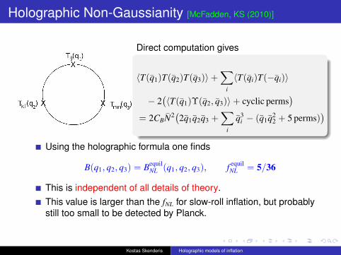
Holographic Non-Gaussianity [McFadden, KS (2010)]

Direct computation gives

〈T(q̄1)T(q̄2)T(q̄3)〉+∑

i

〈T(q̄i)T(−q̄i)〉

− 2(〈T(q̄1)Υ(q̄2, q̄3)〉+ cyclic perms

)= 2CBN̄2(2q̄1q̄2q̄3 +

∑i

q̄3i − (q̄1q̄2

2 + 5 perms))

Using the holographic formula one finds

B(q1, q2, q3) = BequilNL (q1, q2, q3), f equil

NL = 5/36

This is independent of all details of theory.This value is larger than the fNL for slow-roll inflation, but probablystill too small to be detected by Planck.


Tensor Non-Gaussianities [Bzowski, McFadden, KS (2011)]

We computed the complete set of bispecta, involving both scalarand tensor modes.The result a priori could depended in a complicated fashion onthe field content of the dual QFT, but it turns out that we get(nearly) universal results.

These models are predictive.


Conclusions

Standard inflation is holographic: standard observables such aspower spectra and non-Gaussianities can be expressed in termsof (analytic continuation of) correlation functions of a dual QFT.There are new holographic models based on perturbative QFTthat describe a universe that started in a non-geometric stronglycoupled phase.A class of such models based on a super-renormalizable QFTwas custom-fit to data and shown to provide a competitive modelto ΛCDM. Data from the Planck satellite should permit adefinitive test of this holographic scenario.Non-Gaussianity exhibit a universal behavior; the results do notdepend on the details of the dual theory.


Documents

Holographic models of inflation - University of Miami · Holographic universe At the end of this period we arrive at a FRW spacetime and small inhomogeneities with super-horizon correlations