Embed Size (px)
Citation preview
HKL Technology
CHANNEL 4
Revealing Microstructure
HKL Technology ApSAddress : Blåkildevej 17k, DK-9500, Hobro, Denmark.
Tel. : +45 96 57 26 00; Fax. : +45 96 57 26 09
E-mail : [email protected]
Web : www.channel.dk
Important InformationProduct Development
HKL Technology continuously develop their products in line withtechnological advancements and reserve the right to change thedesign and specification of their products without prior notice.Although every care has been taken in the preparation of thisdocument, HKL Technology cannot accept liability for damage orinjury resulting from its use. If users are unsure of any of theinformation presented in this document, particularly with referenceto safety issues, they must contact HKL Technology prior toundertaking any instructions.
Copyright Information© All rights reserved. No part of this publication may bereproduced, stored in a retrieval system or transmitted in any formor by any means without the prior written permission of HKLTechnology ApS.
Author InformationThis manual was written by Austin Day, Klaus Mehnert and BerndtNeumann.
This manual and the accompanying online help file were producedusing Doc-To-Help®, by WexTech Systems, Inc.
Please report any omissions or errors to Austin Day([email protected]).
HKL Technology CHANNEL 4 Contents • i
Contents
General Introduction 1.1
The CHANNEL 4 suite of programs.........................................................1.1Software flexibility and integration...............................................1.2User network, meetings and support .............................................1.2
Installing the CHANNEL 4 software. .......................................................1.3Computer specification .................................................................1.3HASP copy protection...................................................................1.3
Working with Windows ............................................................................1.4CHANNEL 4 - keyboard shortcuts ...........................................................1.4The manuals and help file .........................................................................1.5
Useful background information 2.1
Euler angles ...............................................................................................2.1Euler space ................................................................................................2.3Euler colouring..........................................................................................2.3Specimen directions in terms of angles.....................................................2.5Crystallography – a brief introduction ......................................................2.6
Symmetry ......................................................................................2.6Symmetry of a cube.......................................................................2.6The unit cell...................................................................................2.8
Cubic Crystals ...........................................................................................2.9Cubic unit cell ...............................................................................2.9Directions in a cubic crystal ........................................................2.11Cubic planes and Miller indices ..................................................2.12Cubic formulae............................................................................2.14
Pole figures..............................................................................................2.15Electron backscatter patterns (EBSPs)....................................................2.16
Pattern formation.........................................................................2.16Producing an EBSP .....................................................................2.18
Indexing an Cubic EBSP.........................................................................2.19Match units..................................................................................2.20
CHANNEL EBSD acquisition 3.1
Introduction ...............................................................................................3.1
EBSD - getting started 4.1
Introduction ...............................................................................................4.1Producing and indexing an EBSP .............................................................4.3The cycle control window.........................................................................4.5Argus 20 - EBSP camera control unit .......................................................4.7
ii • Contents HKL Technology CHANNEL 4
Background correction ..................................................................4.7Recommended parameters ..........................................................4.11
Stage and Beam Jobs...............................................................................4.12Introduction .................................................................................4.12External Imaging Processing Delay ............................................4.12Beam Scanning............................................................................4.14Stage Scanning ............................................................................4.15
EBSD system calibration 5.1
Introduction ...............................................................................................5.1Calibration parameters ..............................................................................5.1Calibration guidelines ...............................................................................5.3Calibration procedure................................................................................5.5Calibration refinements .............................................................................5.9
EBSD crystallography 6.1
Defining a crystal structure .......................................................................6.1Creating a CRY file...................................................................................6.4Creating a match unit ................................................................................6.6Critical choice of reflectors used in the match unit...................................6.8
EBSD - running an experiment 7.1
Introduction ...............................................................................................7.1Acquiring an EBSP ...................................................................................7.1Starting CHANNEL - Acquisition and configuring the system................7.3Manually detecting bands..........................................................................7.4Automatically detecting bands ..................................................................7.6Critical choice of cycle control parameters...............................................7.8Indexing patterns .....................................................................................7.12Display of simulation ..............................................................................7.13Principles of pattern indexing .................................................................7.14Pseudosymmetry .....................................................................................7.15Simulating an EBSP for a specific orientation........................................7.17Saving results when finished...................................................................7.18Automatic measurements ........................................................................7.19
Mesotex - misorientations from operator measurements 8.1
Introduction ...............................................................................................8.1
Project manager 9.1
Introduction ...............................................................................................9.1Using Project Manager..............................................................................9.1Attaching to a project ................................................................................9.2Running other programs from Project Manager .......................................9.3
Mambo - (inverse) pole figures 10.1
Introduction .............................................................................................10.1Running Mambo......................................................................................10.1
HKL Technology CHANNEL 4 Contents • iii
Mambo’s toolbar icons............................................................................10.3Reading EBSP orientation data in to Mambo .........................................10.3Displaying a pole figure ..........................................................................10.5The Mambo pop-up menus .....................................................................10.7Creating your own pole figure templates ................................................10.9
Tango - mapping 11.1
Introduction .............................................................................................11.1
Tango - getting started 12.1
Introduction .............................................................................................12.1Running Tango........................................................................................12.1Tango’s toolbar icons ..............................................................................12.3Reading EBSP orientation data in to Tango............................................12.4Using map composer - adding components ............................................12.6Creating a band contrast and zero solution map .....................................12.7The map legend .......................................................................................12.9Noise reduction .....................................................................................12.10Creating an orientation map ..................................................................12.12Misorientation profile............................................................................12.14Line intercept measurements.................................................................12.15Grain reconstruction..............................................................................12.18Deleting a map ......................................................................................12.19General preferences...............................................................................12.19
Tango - map components 13.1
Introduction .............................................................................................13.1Grid components .....................................................................................13.1Boundary components.............................................................................13.3Example component - texture .................................................................13.5
Salsa - orientation distribution functions 14.1
Salsa - Introduction .................................................................................14.1
Salsa - getting started 15.1
Running Salsa..........................................................................................15.1Salsa’s toolbar icons................................................................................15.2Reading EBSP orientation data in to Salsa .............................................15.3Salsa’s 3D-view toolbar icons.................................................................15.4Displaying orientations or misorientations .............................................15.53D-view pop-up menu.............................................................................15.6The (M)ODF preferences tabbed dialog box ..........................................15.8Creating an (M)ODF using the (M)ODF wizard ..................................15.10Deleting an (M)ODF .............................................................................15.13Altering the (M)ODF method and parameters ......................................15.13Reviewing the (M)ODF parameters......................................................15.13Browsing a section through the (M)ODF..............................................15.13Density profile.......................................................................................15.15Viewing serial sections through an (M)ODF ........................................15.16
iv • Contents HKL Technology CHANNEL 4
Texture coefficients...............................................................................15.17Ideal orientations ...................................................................................15.18Creating or altering ideal orientations...................................................15.18
Salsa - introduction to ODF calculations 16.1
Introduction .............................................................................................16.1The result of an (M)ODF calculation..........................................16.2Equivalence of orientation and misorientation............................16.2Determination of misorientation .................................................16.2Coordinate systems .....................................................................16.2
Calculation methods................................................................................16.3Gaussian Kernel Estimation ........................................................16.3Series Expansion Method............................................................16.4Recommended Parameters ..........................................................16.5Comparison of the Calculation Methods.....................................16.5
Subsets 17.1
Subsets - introduction..............................................................................17.1Project manager and subsets ...................................................................17.2Creating a new, empty subset..................................................................17.2Renaming a subset...................................................................................17.2Mambo - adding data to a subset.............................................................17.3Tango - adding individual grains or regions to a subset .........................17.4Salsa - adding data to a subset.................................................................17.5Combining and inverting subsets ............................................................17.7Subset selection from histograms............................................................17.9Saving subset masks..............................................................................17.11Loading subset masks............................................................................17.12Setting the data points of a subset to zero solutions (nullifying) ..........17.12
Open map components (OMC) 18.1
The Concept of open map components ...................................................18.1TaylorCubicX.dll as an example of an OMC..........................................18.2Linking an OMC into Tango...................................................................18.3Writing your own OMC ..........................................................................18.6
Before you start programming ....................................................18.6The Way an OMC is called from within Tango..........................18.7The parameters passed to the OMC ............................................18.7Example OMCs written in Borland Delphi ...........................18.8Example OMCs written in Borland C++ Builder................18.11
Frequently Asked Questions, How Do I ... 19.1
Convert all of my version 3.1 files to the new file format? ....................19.1Highlight a grain in a pole figure or in an ODF? ....................................19.3Determine the percentage of the recrystallized/deformed fraction? .......19.3Display a pole figure / ODF of the recrystallized/deformed fraction?....19.8Display a pole figure / ODF of the small (or the large) grains?............19.10Display a map component for grains of a certain texture component?.19.12Determine the grain size statistics for a certain texture component?....19.16

HKL Technology CHANNEL 4 Contents • v
Determine the percentage of a certain phase in a project?....................19.19Eliminate a phase from a Project?.........................................................19.20Rotate the EBSP data? ..........................................................................19.21Save modified project files?..................................................................19.22Prevent measured data files from being accidentally overwritten?.......19.22
Bibliography 20.1
EBSD measurements and orientation mapping.......................................20.1Crystal data..............................................................................................20.2Introduction to crystallography ...............................................................20.2ODFs and texture analysis.......................................................................20.2
Glossary of terms 21.1
Index 22.1

HKL Technology CHANNEL 4 General Introduction • 1.1
General Introduction
The CHANNEL 4 suite of programsThe CHANNEL 4 suite of programs has been developed to allowyou, the user, to manipulate, analyse and display ElectronBackscatter Diffraction (EBSD) data with comparative ease.
The programs have been designed to be as flexible and extendibleas possible and to allow several users to work independently ortogether on the same computer or over a network.
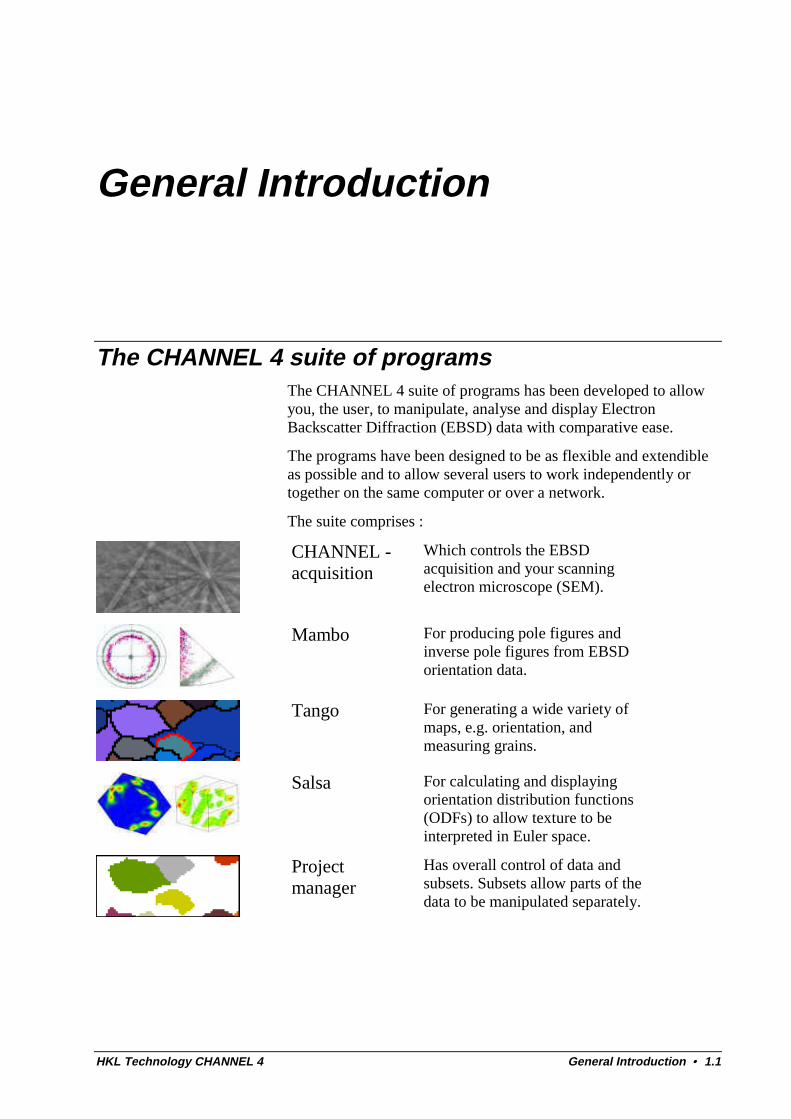
The suite comprises :
CHANNEL -acquisition
Which controls the EBSDacquisition and your scanningelectron microscope (SEM).
Mambo For producing pole figures andinverse pole figures from EBSDorientation data.
Tango For generating a wide variety ofmaps, e.g. orientation, andmeasuring grains.
Salsa For calculating and displayingorientation distribution functions(ODFs) to allow texture to beinterpreted in Euler space.
Projectmanager
Has overall control of data andsubsets. Subsets allow parts of thedata to be manipulated separately.
1.2 • General Introduction HKL Technology CHANNEL 4
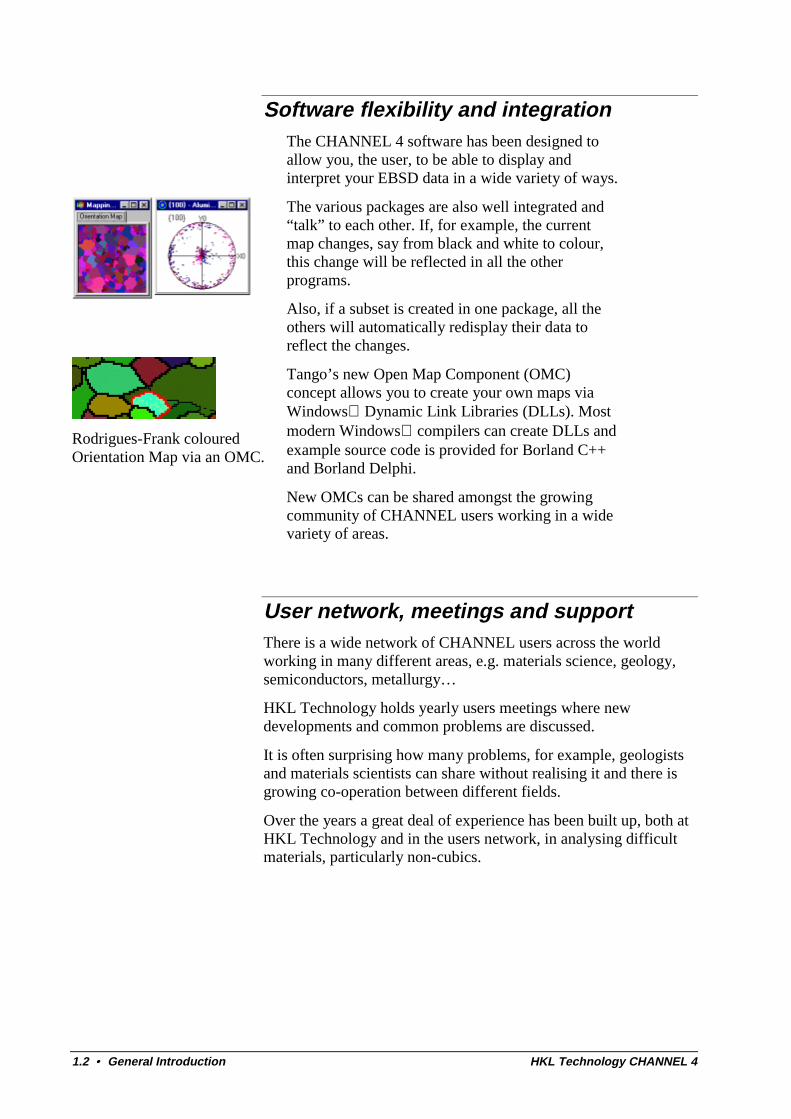
Software flexibility and integrationThe CHANNEL 4 software has been designed toallow you, the user, to be able to display andinterpret your EBSD data in a wide variety of ways.
The various packages are also well integrated and“talk” to each other. If, for example, the currentmap changes, say from black and white to colour,this change will be reflected in all the otherprograms.
Also, if a subset is created in one package, all theothers will automatically redisplay their data toreflect the changes.
Rodrigues-Frank colouredOrientation Map via an OMC.
Tango’s new Open Map Component (OMC)concept allows you to create your own maps viaWindows Dynamic Link Libraries (DLLs). Mostmodern Windows compilers can create DLLs andexample source code is provided for Borland C++and Borland Delphi.
New OMCs can be shared amongst the growingcommunity of CHANNEL users working in a widevariety of areas.
User network, meetings and supportThere is a wide network of CHANNEL users across the worldworking in many different areas, e.g. materials science, geology,semiconductors, metallurgy…
HKL Technology holds yearly users meetings where newdevelopments and common problems are discussed.
It is often surprising how many problems, for example, geologistsand materials scientists can share without realising it and there isgrowing co-operation between different fields.
Over the years a great deal of experience has been built up, both atHKL Technology and in the users network, in analysing difficultmaterials, particularly non-cubics.
HKL Technology CHANNEL 4 General Introduction • 1.3
Installing the CHANNEL 4 software.Insert the supplied CD-ROM in your CD-ROM drive. On mostsystems the installation software will automatically run and leadyou through the installation.
If it does not, then run the program called SETUP.EXE on the CD-ROM and follow the instructions.
Note : As with all software and hardware installations, it is a goodidea to first BACKUP YOUR COMPUTER. Also, keep a recordof Hardware and Hardware Settings (IRQ, I/O, DMA,memory…) before and after installation.
Regular computer backups are important - a lot of effort, time andmoney is spent acquiring data.
Computer specificationThe CHANNEL 4 suite of programs are designed to run on aPersonal Computer (PC) running Windows 95 (release B or above),Windows 98 or Windows NT (service pack 3 or above).
It is recommended that the computer system meets the followingminimum requirements :• 133 MHz Pentium CPU,• 32 Mb of RAM,• Graphics card with 65536 colours at 1280 by 1024 pixies.• 19” Monitor,• Quadruple speed CD-ROM drive,• 200 Mb free hard disk space.
HASP copy protectionThe CHANNEL 4 suite of programs requires a HASP copyprotection dongle to be connected to the printer port or for networkinstallations to a networked computer (NetHASP).
Note : The software will not run without this dongle.
1.4 • General Introduction HKL Technology CHANNEL 4
Working with WindowsIt is assumed that the user is familiar with basic operations inWindows, e.g. clicking and drag-drop. If not, consult yourWindows manual for information and advice.
Moving a Window
All the CHANNEL4 windows can be moved around by clickingon the title bar and dragging the window to a new position.
Tip : Press the Control key to move a window and children.
Resizing a Window
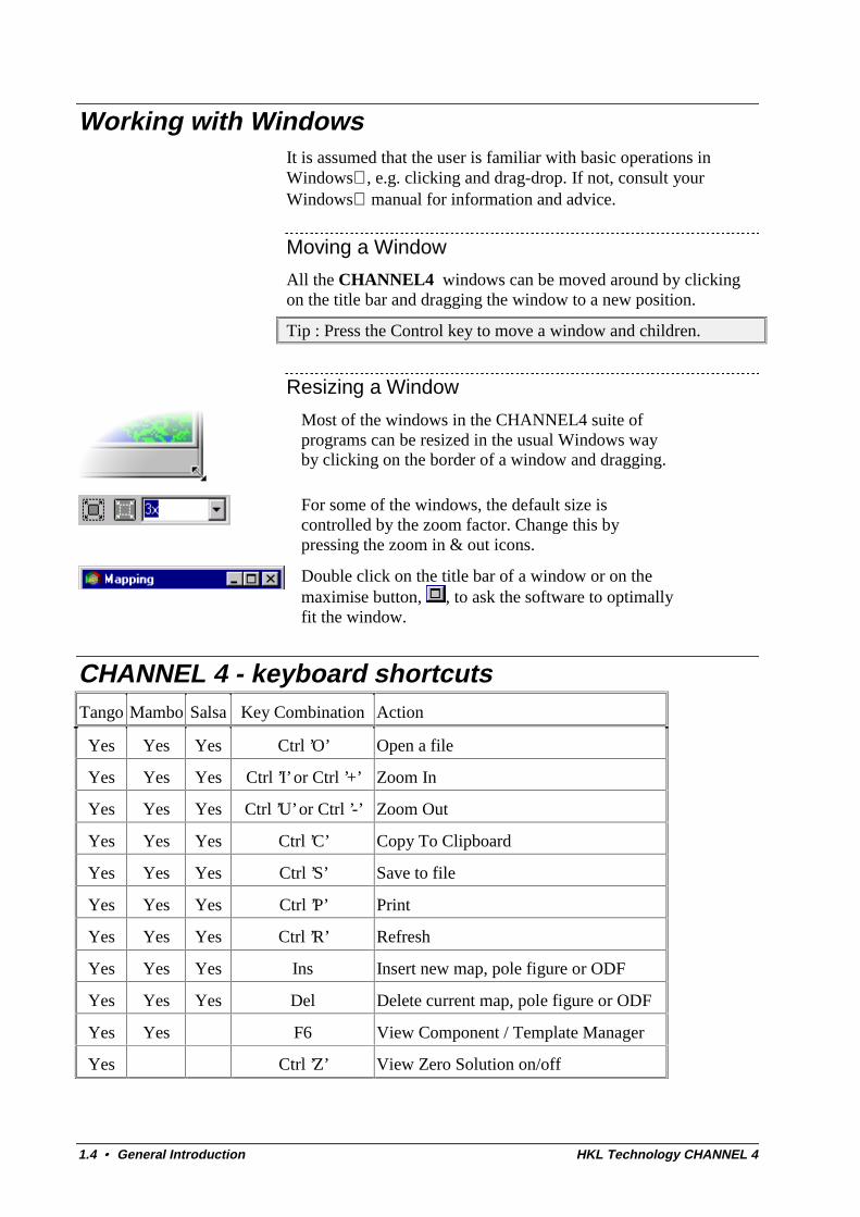
Most of the windows in the CHANNEL4 suite ofprograms can be resized in the usual Windows wayby clicking on the border of a window and dragging.
For some of the windows, the default size iscontrolled by the zoom factor. Change this bypressing the zoom in & out icons.
Double click on the title bar of a window or on themaximise button, , to ask the software to optimallyfit the window.
CHANNEL 4 - keyboard shortcutsTango Mambo Salsa Key Combination Action
Yes Yes Yes Ctrl ’O’ Open a file
Yes Yes Yes Ctrl ’I’ or Ctrl ’+’ Zoom In
Yes Yes Yes Ctrl ’U’ or Ctrl ’-’ Zoom Out
Yes Yes Yes Ctrl ’C’ Copy To Clipboard
Yes Yes Yes Ctrl ’S’ Save to file
Yes Yes Yes Ctrl ’P’ Print
Yes Yes Yes Ctrl ’R’ Refresh
Yes Yes Yes Ins Insert new map, pole figure or ODF
Yes Yes Yes Del Delete current map, pole figure or ODF
Yes Yes F6 View Component / Template Manager
Yes Ctrl ’Z’ View Zero Solution on/off
HKL Technology CHANNEL 4 General Introduction • 1.5
The manuals and help fileWithin these manuals, comments are given in italics, items (e.g.buttons and dialog boxes) in bold italics, and menu items in bold.
Instructions for you, the user, and lists are preceded by a bullet.
Commands using menus are shown in bold, e.g. Project | Openmeans that first the Project menu has to be clicked on, then Open.
Example code is shown in a Courier font.
Tips are shown in boxes, e.g.
Tip : Don’t run with scissors.
Using the Manual and Help file
Have a look in the Glossary section. It has lots of usefulinformation and references back to relevant sections.
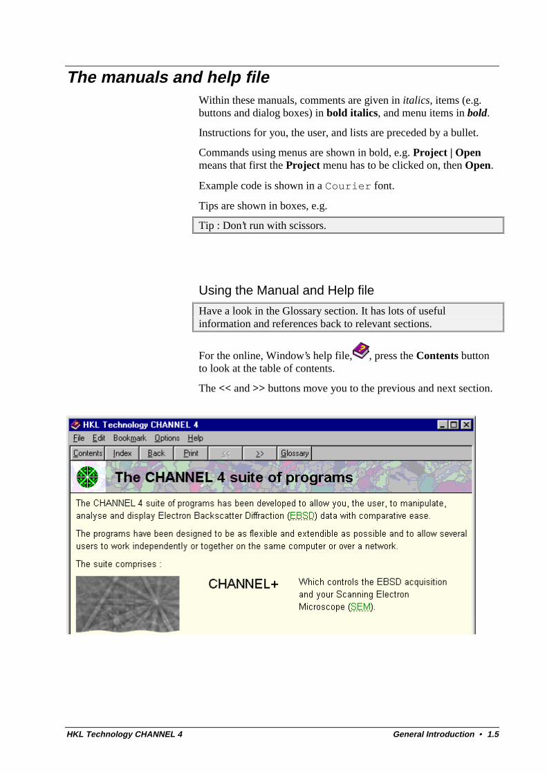
For the online, Window’s help file, , press the Contents buttonto look at the table of contents.
The << and >> buttons move you to the previous and next section.

HKL Technology CHANNEL 4 Useful background information • 2.1
Useful background information
This section contains useful background information.
The section on crystallography is very basic and can be skipped ifnot required. It only really covers cubic crystals (which are easierto explain) although the CHANNEL 4 suite of programs work withall the crystal systems.
Euler anglesEuler angles (Euler 1775) are commonly used to describe a thesample orientation relative to the crystal. This involves rotating oneof the coordinate systems about various axes until it comes intocoincidence with the other.
Different conventions for the choice of axes and angles have beenproposed and applied in literature. For orientation measurements inCHANNEL the convention of Bunge is applied.
Apart from describing crystallite orientations within a specimen,Euler angles are also applied to describe orientation relationshipsbetween other co-ordinate systems used in CHANNEL. The booksby Bunge (1982) and Wenk (1985) contain further useful referenceto texture analysis and the use of Euler angles.
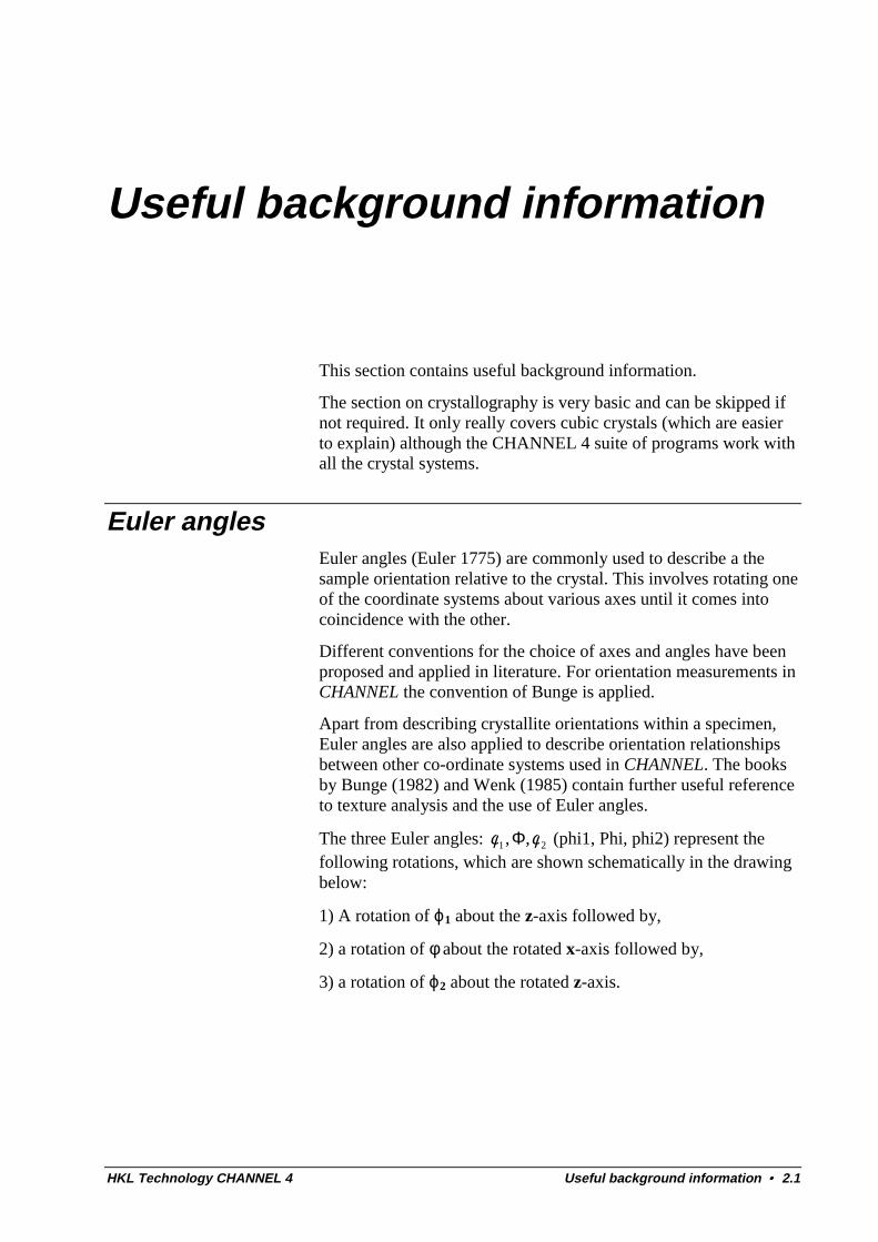
The three Euler angles: 21 ,, φφ Φ (phi1, Phi, phi2) represent thefollowing rotations, which are shown schematically in the drawingbelow:
1) A rotation of ϕ1 about the z-axis followed by,
2) a rotation of φ about the rotated x-axis followed by,
3) a rotation of ϕ2 about the rotated z-axis.
2.2 • Useful background information HKL Technology CHANNEL 4
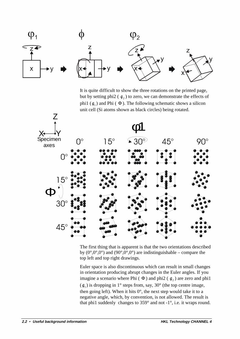
It is quite difficult to show the three rotations on the printed page,but by setting phi2 ( 2φ ) to zero, we can demonstrate the effects of
phi1 ( 1φ ) and Phi ( Φ ). The following schematic shows a siliconunit cell (Si atoms shown as black circles) being rotated.
Z
X YSpecimen
axes
φ1
Φ
��
��
���
���
���
���
���
���
���
The first thing that is apparent is that the two orientations describedby (0°,0°,0°) and (90°,0°,0°) are indistinguishable – compare thetop left and top right drawings.
Euler space is also discontinuous which can result in small changesin orientation producing abrupt changes in the Euler angles. If youimagine a scenario where Phi (Φ ) and phi2 ( 2φ ) are zero and phi1
( 1φ ) is dropping in 1° steps from, say, 30° (the top centre image,then going left). When it hits 0°, the next step would take it to anegative angle, which, by convention, is not allowed. The result isthat phi1 suddenly changes to 359° and not -1°, i.e. it wraps round.
HKL Technology CHANNEL 4 Useful background information • 2.3
N.B. By convention, for cubics, the three Euler angles, 21 ,, φφ Φ ,wrap round at 360°, 90° and 90° respectively.
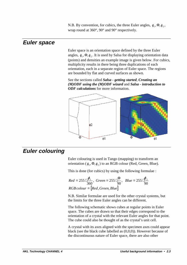
Euler spaceEuler space is an orientation space defined by the three Eulerangles, 21 ,, φφ Φ . It is used by Salsa for displaying orientation data(points) and densities an example image is given below. For cubics,multiplicity results in there being three duplications of eachorientation, each in a separate region of Euler space. The regionsare bounded by flat and curved surfaces as shown.
See the sections called Salsa - getting started, Creating an(M)ODF using the (M)ODF wizard and Salsa - introduction toODF calculations for more information.
Euler colouringEuler colouring is used in Tango (mapping) to transform anorientation ( 21 ,, φφ Φ ) to an RGB colour (Red, Green, Blue).
This is done (for cubics) by using the following formulae :
[ ]BlueGreenRedcolourRGB
BlueGreenRed
,,90
255,90
255,360
255 21
=
⋅=Φ⋅=⋅= ϕϕ
N.B. Similar formulae are used for the other crystal systems, butthe limits for the three Euler angles can be different.
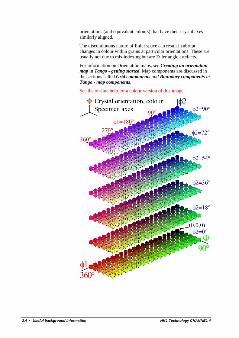
The following schematic shows cubes at regular points in Eulerspace. The cubes are drawn so that their edges correspond to theorientation of a crystal with the relevant Euler angles for that point.The cube could also be thought of as the crystal’s unit cell.
A crystal with its axes aligned with the specimen axes could appearblack (see the black cube labelled as (0,0,0)). However because ofthe discontinuous nature of Euler space, there are also other
2.4 • Useful background information HKL Technology CHANNEL 4
orientations (and equivalent colours) that have their crystal axessimilarly aligned.
The discontinuous nature of Euler space can result in abruptchanges in colour within grains at particular orientations. These areusually not due to mis-indexing but are Euler angle artefacts.
For information on Orientation maps, see Creating an orientationmap in Tango - getting started. Map components are discussed inthe sections called Grid components and Boundary components inTango - map components.
See the on-line help for a colour version of this image.
HKL Technology CHANNEL 4 Useful background information • 2.5
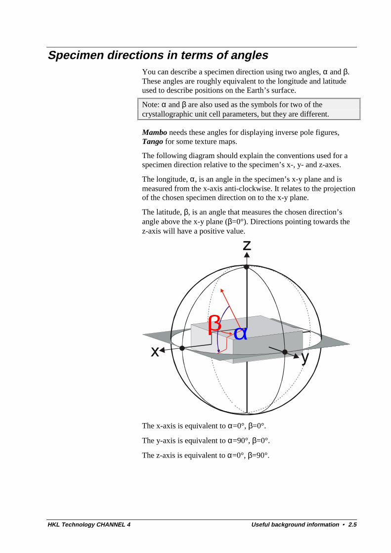
Specimen directions in terms of anglesYou can describe a specimen direction using two angles, α and β.These angles are roughly equivalent to the longitude and latitudeused to describe positions on the Earth’s surface.
Note: α and β are also used as the symbols for two of thecrystallographic unit cell parameters, but they are different.
Mambo needs these angles for displaying inverse pole figures,Tango for some texture maps.
The following diagram should explain the conventions used for aspecimen direction relative to the specimen’s x-, y- and z-axes.
The longitude, α, is an angle in the specimen’s x-y plane and ismeasured from the x-axis anti-clockwise. It relates to the projectionof the chosen specimen direction on to the x-y plane.
The latitude, β, is an angle that measures the chosen direction’sangle above the x-y plane (β=0°). Directions pointing towards thez-axis will have a positive value.
αβ
The x-axis is equivalent to α=0°, β=0°.
The y-axis is equivalent to α=90°, β=0°.
The z-axis is equivalent to α=0°, β=90°.
2.6 • Useful background information HKL Technology CHANNEL 4
Crystallography – a brief introductionThe regular arrangement of atoms in a crystal, called a lattice, canbe described mathematically by repeating a small piece of thecrystal called the basis. The way that the basis has to be repeated isdefined by a regular volume called the unit cell.
For any given crystal there are many possible unit cells, but thesimplest one is usually chosen such that it contains a minimumnumber of atoms but still displays the symmetry of the crystallattice.
This chapter is designed to be a very basic introduction tocrystallography. The Bibliography contains several references tobooks that have more information on crystallography.
SymmetrySymmetry is very important to crystals and can allow thearrangements of their atoms to be described in a form of shorthand.A symmetry operation is an action on an object that doessomething to the object but leaves it essentially unchanged. Thismay seem to be a very vague concept but it is surprisingly powerfuland is fundamental to crystallography.
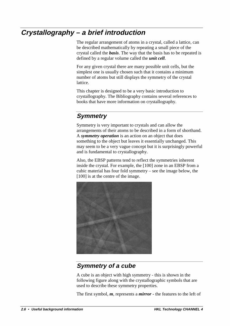
Also, the EBSP patterns tend to reflect the symmetries inherentinside the crystal. For example, the [100] zone in an EBSP from acubic material has four fold symmetry – see the image below, the[100] is at the centre of the image.
Symmetry of a cubeA cube is an object with high symmetry - this is shown in thefollowing figure along with the crystallographic symbols that areused to describe these symmetry properties.
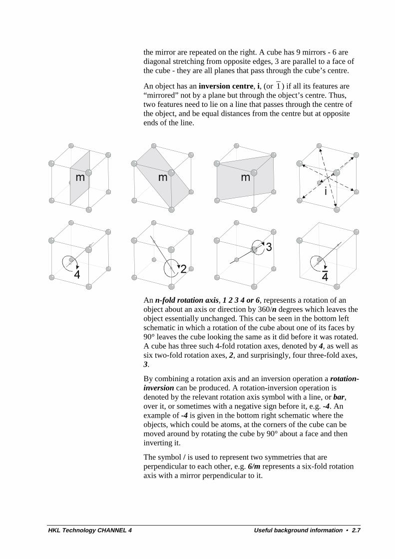
The first symbol, m, represents a mirror - the features to the left of
HKL Technology CHANNEL 4 Useful background information • 2.7
the mirror are repeated on the right. A cube has 9 mirrors - 6 arediagonal stretching from opposite edges, 3 are parallel to a face ofthe cube - they are all planes that pass through the cube’s centre.
An object has an inversion centre, i, (or 1 ) if all its features are“mirrored” not by a plane but through the object’s centre. Thus,two features need to lie on a line that passes through the centre ofthe object, and be equal distances from the centre but at oppositeends of the line.
An n-fold rotation axis, 1 2 3 4 or 6, represents a rotation of anobject about an axis or direction by 360/n degrees which leaves theobject essentially unchanged. This can be seen in the bottom leftschematic in which a rotation of the cube about one of its faces by90° leaves the cube looking the same as it did before it was rotated.A cube has three such 4-fold rotation axes, denoted by 4, as well assix two-fold rotation axes, 2, and surprisingly, four three-fold axes,3.
By combining a rotation axis and an inversion operation a rotation-inversion can be produced. A rotation-inversion operation isdenoted by the relevant rotation axis symbol with a line, or bar,over it, or sometimes with a negative sign before it, e.g. -4. Anexample of -4 is given in the bottom right schematic where theobjects, which could be atoms, at the corners of the cube can bemoved around by rotating the cube by 90° about a face and theninverting it.
The symbol / is used to represent two symmetries that areperpendicular to each other, e.g. 6/m represents a six-fold rotationaxis with a mirror perpendicular to it.
2.8 • Useful background information HKL Technology CHANNEL 4
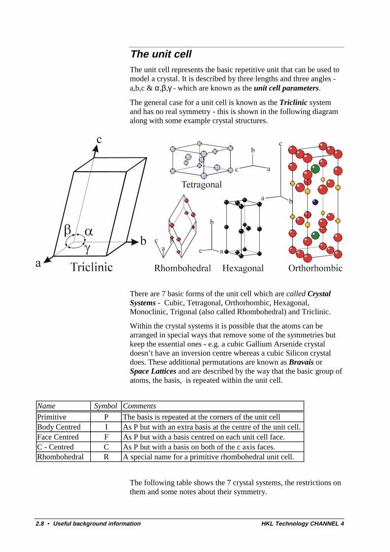
The unit cellThe unit cell represents the basic repetitive unit that can be used tomodel a crystal. It is described by three lengths and three angles -a,b,c & α,β,γ - which are known as the unit cell parameters.
The general case for a unit cell is known as the Triclinic systemand has no real symmetry - this is shown in the following diagramalong with some example crystal structures.
There are 7 basic forms of the unit cell which are called CrystalSystems - Cubic, Tetragonal, Orthorhombic, Hexagonal,Monoclinic, Trigonal (also called Rhombohedral) and Triclinic.
Within the crystal systems it is possible that the atoms can bearranged in special ways that remove some of the symmetries butkeep the essential ones - e.g. a cubic Gallium Arsenide crystaldoesn’t have an inversion centre whereas a cubic Silicon crystaldoes. These additional permutations are known as Bravais orSpace Lattices and are described by the way that the basic group ofatoms, the basis, is repeated within the unit cell.
Name Symbol Comments
Primitive P The basis is repeated at the corners of the unit cellBody Centred I As P but with an extra basis at the centre of the unit cell.Face Centred F As P but with a basis centred on each unit cell face.C - Centred C As P but with a basis on both of the c axis faces.Rhombohedral R A special name for a primitive rhombohedral unit cell.
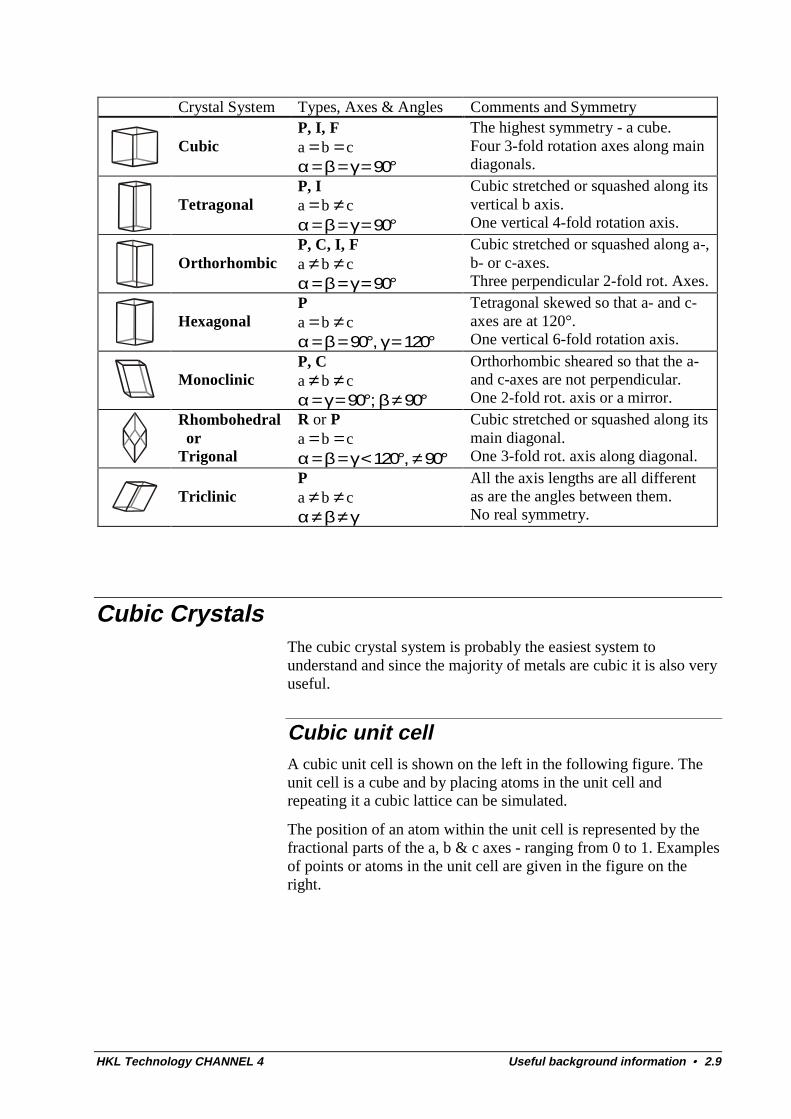
The following table shows the 7 crystal systems, the restrictions onthem and some notes about their symmetry.
HKL Technology CHANNEL 4 Useful background information • 2.9
Crystal System Types, Axes & Angles Comments and Symmetry
CubicP, I, Fa = b = cα = β = γ = 90°
The highest symmetry - a cube.Four 3-fold rotation axes along maindiagonals.
TetragonalP, Ia = b ≠ cα = β = γ = 90°
Cubic stretched or squashed along itsvertical b axis.One vertical 4-fold rotation axis.
OrthorhombicP, C, I, Fa ≠ b ≠ cα = β = γ = 90°
Cubic stretched or squashed along a-,b- or c-axes.Three perpendicular 2-fold rot. Axes.
HexagonalPa = b ≠ cα = β = 90°, γ = 120°
Tetragonal skewed so that a- and c-axes are at 120°.One vertical 6-fold rotation axis.
MonoclinicP, Ca ≠ b ≠ cα = γ = 90°; β ≠ 90°
Orthorhombic sheared so that the a-and c-axes are not perpendicular.One 2-fold rot. axis or a mirror.
Rhombohedral orTrigonal
R or Pa = b = cα = β = γ < 120°, ≠ 90°
Cubic stretched or squashed along itsmain diagonal.One 3-fold rot. axis along diagonal.
TriclinicPa ≠ b ≠ cα ≠ β ≠ γ
All the axis lengths are all differentas are the angles between them.No real symmetry.
Cubic CrystalsThe cubic crystal system is probably the easiest system tounderstand and since the majority of metals are cubic it is also veryuseful.
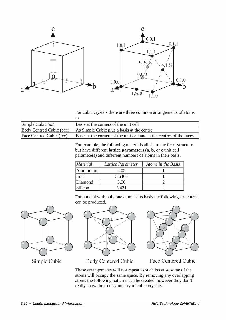
Cubic unit cellA cubic unit cell is shown on the left in the following figure. Theunit cell is a cube and by placing atoms in the unit cell andrepeating it a cubic lattice can be simulated.
The position of an atom within the unit cell is represented by thefractional parts of the a, b & c axes - ranging from 0 to 1. Examplesof points or atoms in the unit cell are given in the figure on theright.
2.10 • Useful background information HKL Technology CHANNEL 4
For cubic crystals there are three common arrangements of atoms:::
Simple Cubic (sc) Basis at the corners of the unit cellBody Centred Cubic (bcc) As Simple Cubic plus a basis at the centreFace Centred Cubic (fcc) Basis at the corners of the unit cell and at the centres of the faces
For example, the following materials all share the f.c.c. structurebut have different lattice parameters (a, b, or c unit cellparameters) and different numbers of atoms in their basis.
Material Lattice Parameter Atoms in the Basis
Aluminium 4.05 1Iron 3.6468 1Diamond 3.56 2Silicon 5.431 2
For a metal with only one atom as its basis the following structurescan be produced.
These arrangements will not repeat as such because some of theatoms will occupy the same space. By removing any overlappingatoms the following patterns can be created, however they don’treally show the true symmetry of cubic crystals.
HKL Technology CHANNEL 4 Useful background information • 2.11
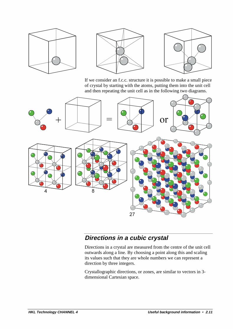
If we consider an f.c.c. structure it is possible to make a small pieceof crystal by starting with the atoms, putting them into the unit celland then repeating the unit cell as in the following two diagrams.
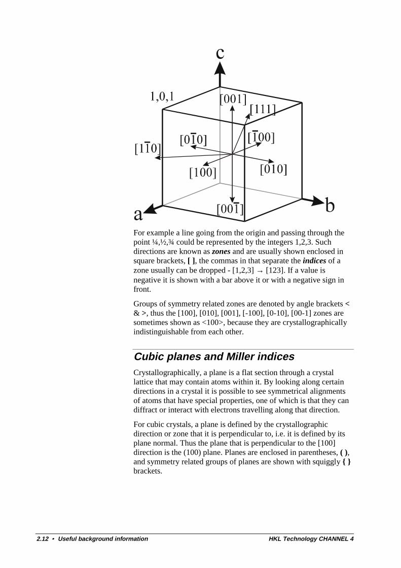
Directions in a cubic crystalDirections in a crystal are measured from the centre of the unit celloutwards along a line. By choosing a point along this and scalingits values such that they are whole numbers we can represent adirection by three integers.
Crystallographic directions, or zones, are similar to vectors in 3-dimensional Cartesian space.
2.12 • Useful background information HKL Technology CHANNEL 4
For example a line going from the origin and passing through thepoint ¼,½,¾ could be represented by the integers 1,2,3. Suchdirections are known as zones and are usually shown enclosed insquare brackets, [ ], the commas in that separate the indices of azone usually can be dropped - [1,2,3] → [123]. If a value isnegative it is shown with a bar above it or with a negative sign infront.
Groups of symmetry related zones are denoted by angle brackets <& >, thus the [100], [010], [001], [-100], [0-10], [00-1] zones aresometimes shown as <100>, because they are crystallographicallyindistinguishable from each other.
Cubic planes and Miller indicesCrystallographically, a plane is a flat section through a crystallattice that may contain atoms within it. By looking along certaindirections in a crystal it is possible to see symmetrical alignmentsof atoms that have special properties, one of which is that they candiffract or interact with electrons travelling along that direction.
For cubic crystals, a plane is defined by the crystallographicdirection or zone that it is perpendicular to, i.e. it is defined by itsplane normal. Thus the plane that is perpendicular to the [100]direction is the (100) plane. Planes are enclosed in parentheses, ( ),and symmetry related groups of planes are shown with squiggly { }brackets.
HKL Technology CHANNEL 4 Useful background information • 2.13
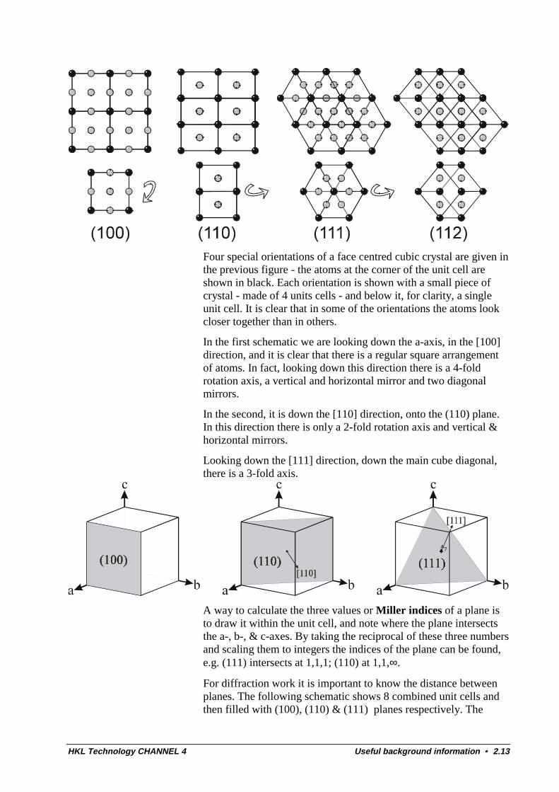
Four special orientations of a face centred cubic crystal are given inthe previous figure - the atoms at the corner of the unit cell areshown in black. Each orientation is shown with a small piece ofcrystal - made of 4 units cells - and below it, for clarity, a singleunit cell. It is clear that in some of the orientations the atoms lookcloser together than in others.
In the first schematic we are looking down the a-axis, in the [100]direction, and it is clear that there is a regular square arrangementof atoms. In fact, looking down this direction there is a 4-foldrotation axis, a vertical and horizontal mirror and two diagonalmirrors.
In the second, it is down the [110] direction, onto the (110) plane.In this direction there is only a 2-fold rotation axis and vertical &horizontal mirrors.
Looking down the [111] direction, down the main cube diagonal,there is a 3-fold axis.
A way to calculate the three values or Miller indices of a plane isto draw it within the unit cell, and note where the plane intersectsthe a-, b-, & c-axes. By taking the reciprocal of these three numbersand scaling them to integers the indices of the plane can be found,e.g. (111) intersects at 1,1,1; (110) at 1,1,∞.
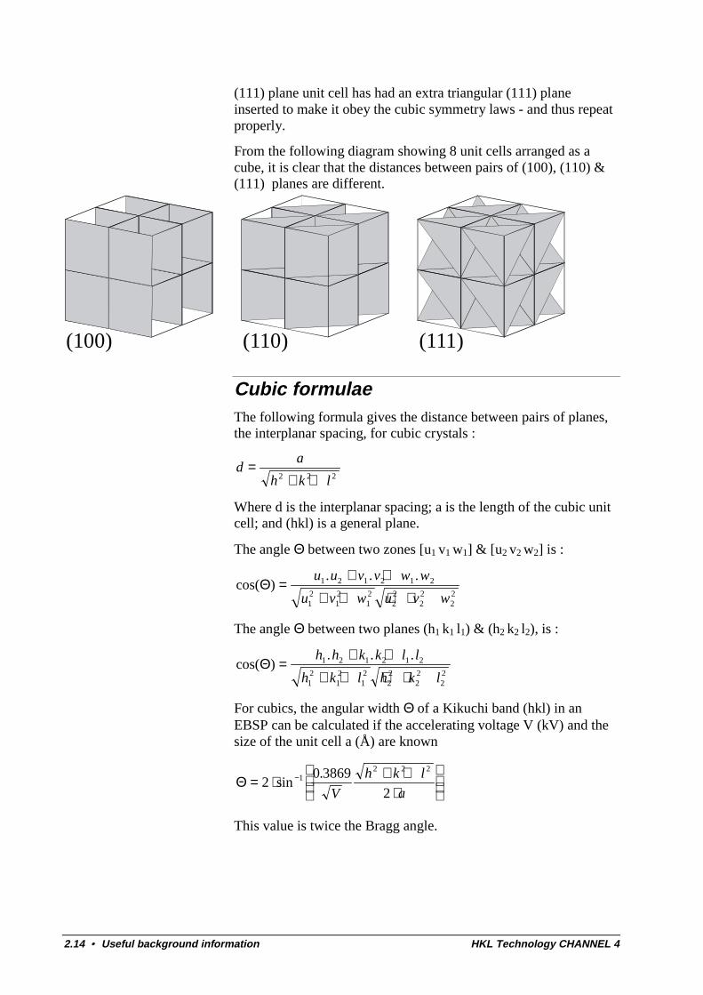
For diffraction work it is important to know the distance betweenplanes. The following schematic shows 8 combined unit cells andthen filled with (100), (110) & (111) planes respectively. The
2.14 • Useful background information HKL Technology CHANNEL 4
(111) plane unit cell has had an extra triangular (111) planeinserted to make it obey the cubic symmetry laws - and thus repeatproperly.
From the following diagram showing 8 unit cells arranged as acube, it is clear that the distances between pairs of (100), (110) &(111) planes are different.
(100) (110) (111)
Cubic formulaeThe following formula gives the distance between pairs of planes,the interplanar spacing, for cubic crystals :
da
h k l=
+ +2 2 2
Where d is the interplanar spacing; a is the length of the cubic unitcell; and (hkl) is a general plane.
The angle Θ between two zones [u1 v1 w1] & [u2 v2 w2] is :
cos( ). . .
Θ =+ +
+ + + +u u v v w w
u v w u v w1 2 1 2 1 2
12
12
12
22
22
22
The angle Θ between two planes (h1 k1 l1) & (h2 k2 l2), is :
cos( ). . .
Θ =+ +
+ + + +h h k k l l
h k l h k l1 2 1 2 1 2
12
12
12
22
22
22
For cubics, the angular width Θ of a Kikuchi band (hkl) in anEBSP can be calculated if the accelerating voltage V (kV) and thesize of the unit cell a (Å) are known
Θ = ⋅ + +⋅
−20 3869
21
2 2 2
sin.
V
h k l
a
This value is twice the Bragg angle.
HKL Technology CHANNEL 4 Useful background information • 2.15
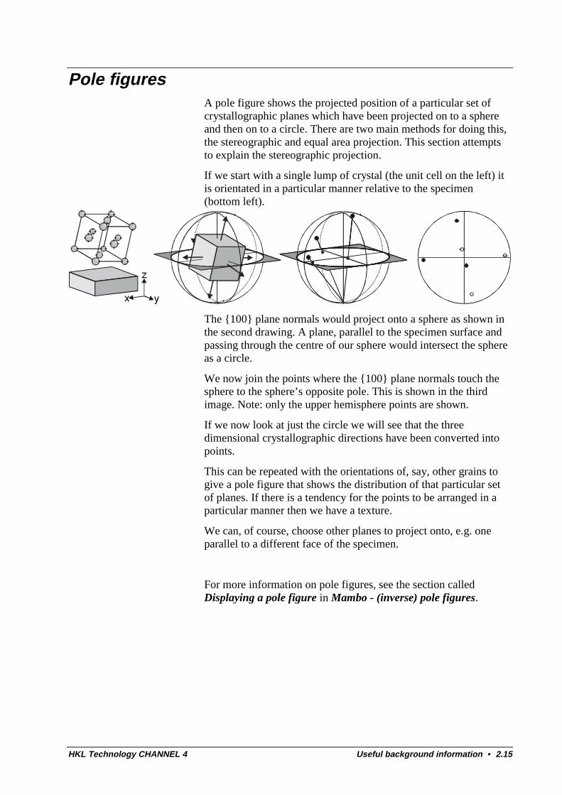
Pole figuresA pole figure shows the projected position of a particular set ofcrystallographic planes which have been projected on to a sphereand then on to a circle. There are two main methods for doing this,the stereographic and equal area projection. This section attemptsto explain the stereographic projection.
If we start with a single lump of crystal (the unit cell on the left) itis orientated in a particular manner relative to the specimen(bottom left).
The {100} plane normals would project onto a sphere as shown inthe second drawing. A plane, parallel to the specimen surface andpassing through the centre of our sphere would intersect the sphereas a circle.
We now join the points where the {100} plane normals touch thesphere to the sphere’s opposite pole. This is shown in the thirdimage. Note: only the upper hemisphere points are shown.
If we now look at just the circle we will see that the threedimensional crystallographic directions have been converted intopoints.
This can be repeated with the orientations of, say, other grains togive a pole figure that shows the distribution of that particular setof planes. If there is a tendency for the points to be arranged in aparticular manner then we have a texture.
We can, of course, choose other planes to project onto, e.g. oneparallel to a different face of the specimen.
For more information on pole figures, see the section calledDisplaying a pole figure in Mambo - (inverse) pole figures.
2.16 • Useful background information HKL Technology CHANNEL 4
Electron backscatter patterns (EBSPs)An Electron Back-Scattering Pattern (EBSP) consists of manyintersecting, linear features called Kikuchi bands - which consist ofa strip, brighter than the background, bounded by two edges. Eachedge is geometrically attributable to electrons that have beendiffracted from a particular plane of atoms within the specimen.
EBSPs are also known as Kikuchi patterns. The technique itselfhas a variety of names - electron backscatter diffraction (EBSD),back-scatter Kikuchi diffraction (BKD) and back-scatteredelectron Kikuchi diffraction (BEKD). There are a variety ofspellings of the word backscatter : back-scatter, backscatter andeven backscattering and backscattered.
Kikuchi patterns were first observed by Kikuchi in theTransmission Electron Microscope [Diffraction of Kathode Rays byMica, S. Kikuchi, Imp. Acad. Tokyo, Proc., June 1928, Volume 4,pages 271-278.] Kikuchi found that electron diffraction patternsfrom thin films of mica contained the expected diffraction spots ona background of linear structures which consisted of pairs ofparallel ‘excess’ and ‘defect’ lines, now known as Kikuchi lines.
The positions of the Kikuchi lines could be explained on purelygeometric grounds from a knowledge of Bragg diffraction fromcrystal planes. The angular range of these patterns was only 15°.Between the lines are regions that are brighter than the background,these are called Kikuchi Bands.
With modern EBSD systems the capture is about 60°, which for acubic EBSP is the distance between two neighbouring <110>zones.
Pattern formationThe exact method of pattern formation is not well understood,although structure factor calculations (see glossary entry) allow therelative intensities of the Kikuchi bands to be calculated.
The formation of an EBSP can be described as follows :
a) The electrons strike the specimen, and within the pattern sourcepoint (PSP) they are inelastically scattered, losing ~1% of theirenergy - this produces a little line broadening.
b) These scattering events generate electrons travelling in allconceivable directions in a small volume which is effectively apoint source.
HKL Technology CHANNEL 4 Useful background information • 2.17
c) Electrons that satisfy the Bragg diffraction condition (seeGlossary entry) for a particular plane are channeled differently tothe other electrons - thus producing a change in intensity.
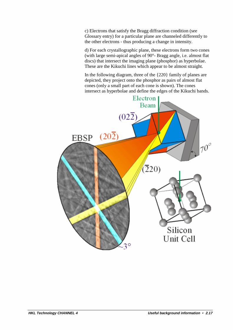
d) For each crystallographic plane, these electrons form two cones(with large semi-apical angles of 90°- Bragg angle, i.e. almost flatdiscs) that intersect the imaging plane (phosphor) as hyperbolae.These are the Kikuchi lines which appear to be almost straight.
In the following diagram, three of the {220} family of planes aredepicted, they project onto the phosphor as pairs of almost flatcones (only a small part of each cone is shown). The conesintersect as hyperbolae and define the edges of the Kikuchi bands.
2.18 • Useful background information HKL Technology CHANNEL 4
Producing an EBSP
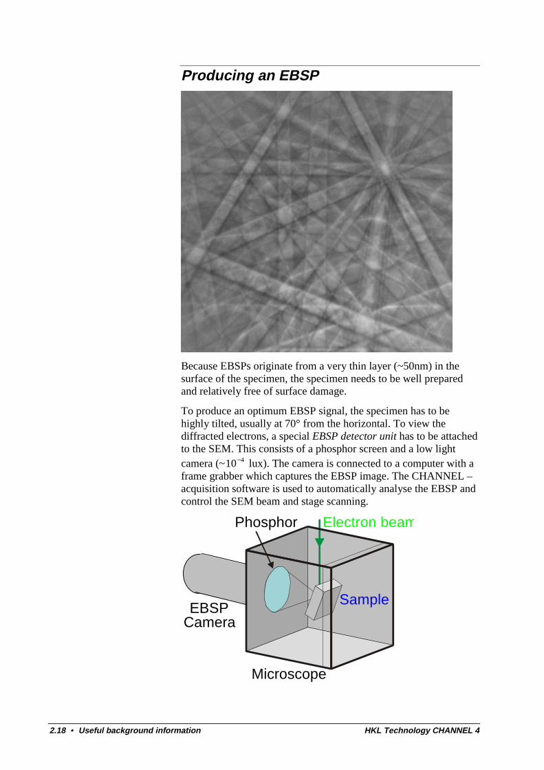
Because EBSPs originate from a very thin layer (~50nm) in thesurface of the specimen, the specimen needs to be well preparedand relatively free of surface damage.
To produce an optimum EBSP signal, the specimen has to behighly tilted, usually at 70° from the horizontal. To view thediffracted electrons, a special EBSP detector unit has to be attachedto the SEM. This consists of a phosphor screen and a low lightcamera (~ 410− lux). The camera is connected to a computer with aframe grabber which captures the EBSP image. The CHANNEL –acquisition software is used to automatically analyse the EBSP andcontrol the SEM beam and stage scanning.
EBSPCamera
Phosphor Electron beam
Sample
Microscope
HKL Technology CHANNEL 4 Useful background information • 2.19
See the Glossary entry for EBSD and the section calledCHANNEL EBSD acquisition for an introduction, and Producingand indexing an EBSP and Principles of pattern indexing formore details.
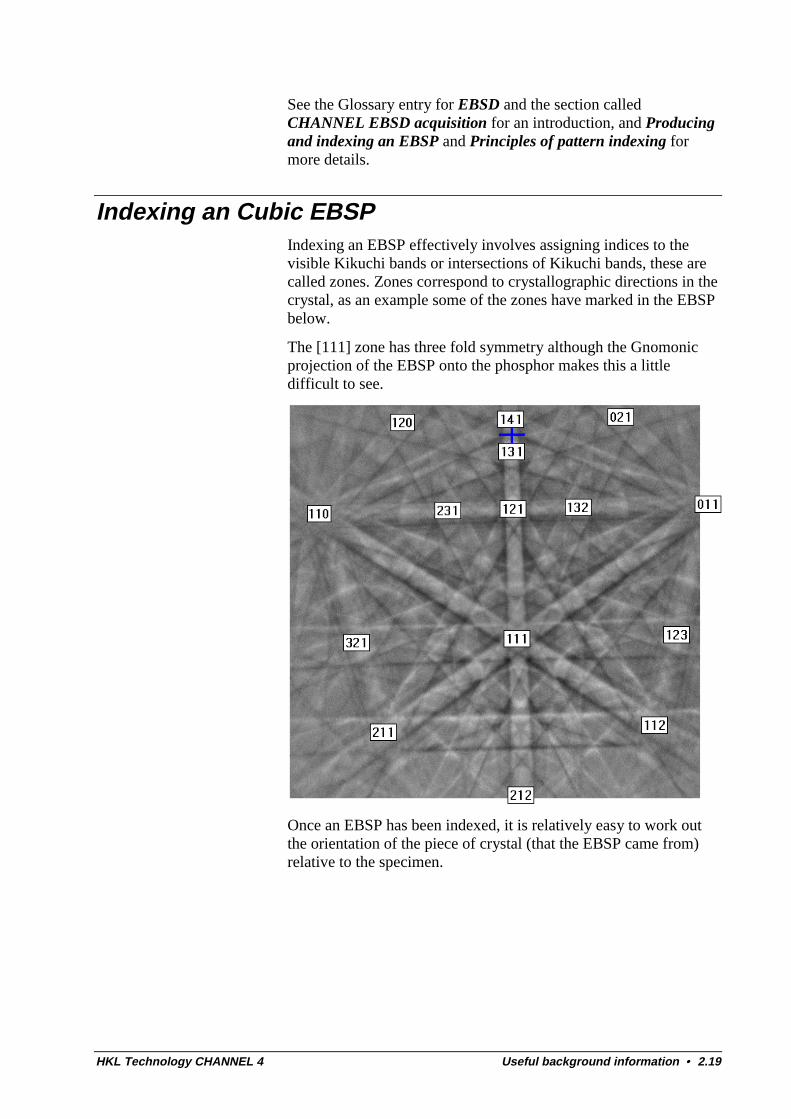
Indexing an Cubic EBSPIndexing an EBSP effectively involves assigning indices to thevisible Kikuchi bands or intersections of Kikuchi bands, these arecalled zones. Zones correspond to crystallographic directions in thecrystal, as an example some of the zones have marked in the EBSPbelow.
The [111] zone has three fold symmetry although the Gnomonicprojection of the EBSP onto the phosphor makes this a littledifficult to see.
Once an EBSP has been indexed, it is relatively easy to work outthe orientation of the piece of crystal (that the EBSP came from)relative to the specimen.

2.20 • Useful background information HKL Technology CHANNEL 4
Match unitsWhen the CHANNEL – acquisition software automatically indexesan EBSP, it needs crystallographic data and lists of Kikuchi bandsfor each of the phases it is looking for. This data is defined in amatch unit. It is relatively easy to create and in a lot of cases thedata already exists.
Sometimes, it is possible to use crystallographic data from similarmaterials, e.g. aluminium data could be used for an f.c.c.superalloy. The crystallographic data is stored in a file with the.CRY file extension.
The list of the Kikuchi bands and their relative intensities can becalculated using CHANNEL – acquisition and stored in a matchunit (with the file extension .HKL).
For information on creating a .CRY file, see the sections calledDefining a crystal structure and Creating a CRY file in EBSDcrystallography.
For information on creating a Match unit, see the sections calledCreating a match unit, Critical choice of reflectors used in thematch unit and Principles of pattern indexing in EBSDcrystallography.
HKL Technology CHANNEL 4 CHANNEL EBSD acquisition • 3.1
CHANNEL EBSD acquisition
Introduction
Crystallographic measurements and EBSD
An important feature in materials analysis is the study ofcrystallographic structures of the constituting grains crystalliteswithin a solid which directly relate to its physical properties. Manymaterials, especially after processing, acquire a preferredorientation i.e. a non-random orientation of the single crystallattices which is called a texture and which is related to thematerials properties on a bulk scale. The traditional approach toinvestigate preferred orientations in a solid is to determine theglobal texture, i.e. the statistical distribution of crystalliteorientations averaged over a measured sample volume by x-ray orneutron diffraction experiments. However, the disadvantage ofthese techniques is the missing link to observations made on themicrostructure, i.e. the distribution, size and shape of crystallitesfrom the constituting phases of the solid. On the other handcrystallographic data from electron diffraction in the transmissionelectron microscope (TEM) is too limited in amount to account forstatistically significant texture analyses.
Through the development of electron diffraction techniques in thescanning electron microscope (SEM) it became feasible to observeboth the microstructure and texture within large specimen. Thesetechniques are thus also able to reveal the local texture, i.e. thedistribution of single crystallite orientations with respect to themicrostructure as well as their orientation relationships andmisorientations at microstructural interfaces (phase-, grain-,subgrain-, twin boundaries, fractures etc.).
The most common and modern method to measure singlecrystallite orientations in a microstructural framework is theanalysis of electron backscatter patterns (EBSP) in the SEM,which was first used by Venables & Harland (1973). EBSPsconsist of relatively intense bands (Kikuchi bands) intersecting oneanother and overlying the normal distribution of backscattered
3.2 • CHANNEL EBSD acquisition HKL Technology CHANNEL 4
electrons. These patterns are sometimes also referred to asbackscatter Kikuchi patterns (BSKP, named after Kikuchi, 1928,who first observed similar diffraction patterns in the TEM). Theyare the result of Bragg diffraction of electrons at all atomic planesin the crystal lattice and occur in a very thin layer (<50nm) in thesurface of the specimen which consequently has to be free of anymechanical damage produced by grinding and polishing. Toproduce an optimum EBSP signal in the SEM, the specimen has tobe highly tilted (50-80°) from the horizonal. Therefore a specialEBSP detector unit has to be attached to the SEM which consists ofa phosphor screen to image the EBSPs and a low light video-camera to view them.
How CHANNEL - Acquisition operates
CHANNEL - Acquisition is used to analyse the crystallographictexture of a material by means of single crystallite orientationsderived from EBSPs as described above. CHANNEL - Acquisitionutilises an image capture board (frame grabber) to read the camerasTV rate signal from the EBSP detector unit and then displays it onthe monitor with a graphics overlay.
During the measurements the positions of Kikuchi bands in anEBSP can either be detected automatically or be entered manuallyby the operator. The program will then present the operator with anindexing, i.e. a simulation of Kikuchi bands, which represents themost likely solution of phase and orientation that matches the inputdata. The resulting phase and orientation data is finally stored in afile for further processing of orientation or misorientation data.

HKL Technology CHANNEL 4 CHANNEL EBSD acquisition • 3.3
User and EBSD requirements
It is assumed that you, the user, are familiar with the safe operationof your Scanning Electron Microscope (SEM) and relatedequipment and have the following :
a) Basic SEM skills, e.g. focussing, specimen movement, changingmagnification producing images and switching to spot mode. If anyof these are unfamiliar please refer to your SEM manuals.
b) A basic knowledge of the Windows™ environment.
c) Basic EBSD specimen preparation skills or assistance fromsomeone with such skills.
d) A basic understanding of crystallography.
If you feel you cannot satisfy the above requirements then pleaseapproach your SEM and computer support personnel or contactHKL Technology before using the system.
N.B. We hold annual User Meetings and can provide training ifrequired.

HKL Technology CHANNEL 4 EBSD - getting started • 4.1
EBSD - getting started
IntroductionThis section gives you an introduction to using CHANNEL -Acquisition and is designed to get a new user started. It is a brief,step by step guide to using the software to produce crystallographicorientation measurements from a prepared specimen. It follows theorder of operational procedures given in detail in the section called“EBSD - running an experiment” and covers the most importantitems in a quick overview.
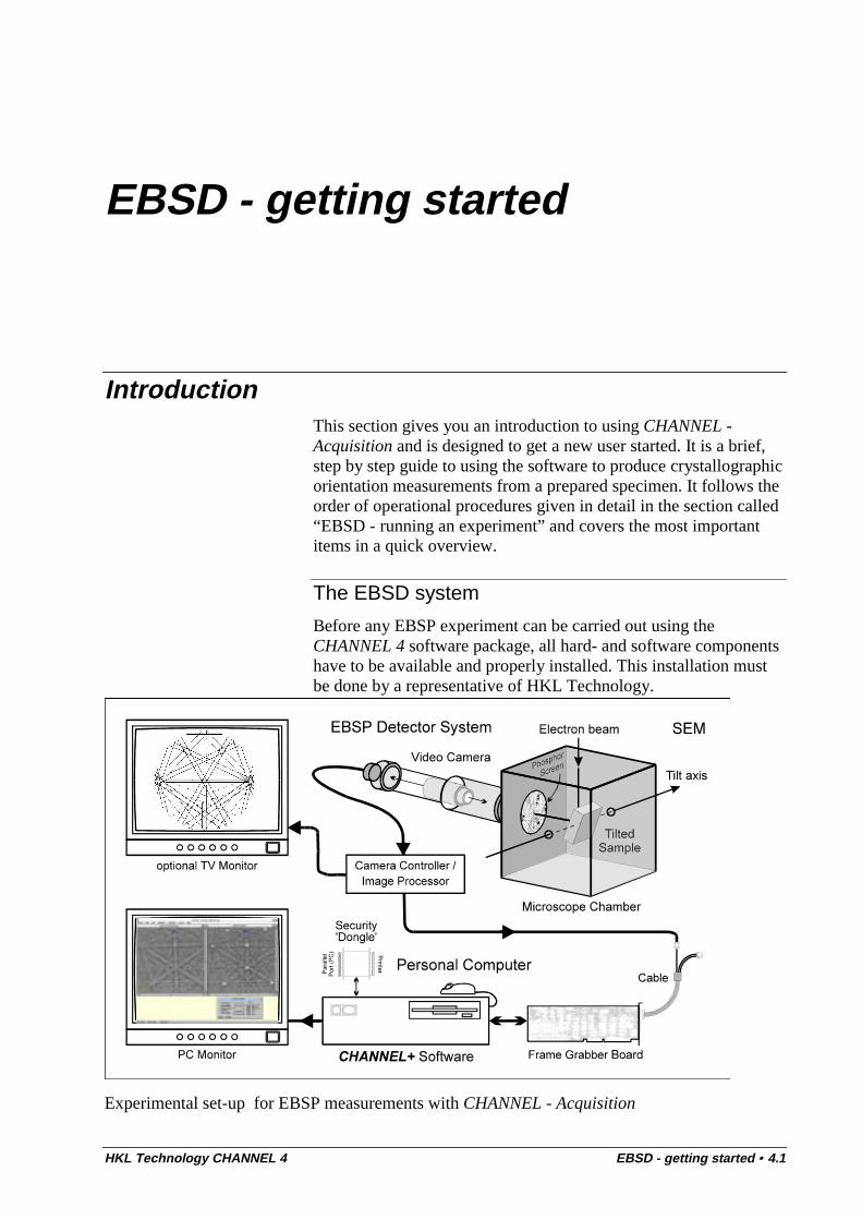
The EBSD system
Before any EBSP experiment can be carried out using theCHANNEL 4 software package, all hard- and software componentshave to be available and properly installed. This installation mustbe done by a representative of HKL Technology.
Experimental set-up for EBSP measurements with CHANNEL - Acquisition
4.2 • EBSD - getting started HKL Technology CHANNEL 4
Calibrating the system
The purpose of calibrating the EBSP system is to establish thegeometrical relationships between SEM, EBSP detector and thepattern projection which is critical for obtaining reliable orientationdata.
If CHANNEL - Acquisition has been professionally installed andconfigured then it is likely that the existing calibration will be validfor the first orientation measurements, given that the SEMoperation conditions are the same.
In general the EBSP system has to be calibrated each time theoperating conditions (e.g. acceleration voltage, working distance)are changed. The calibration parameters can be saved to acalibration file (*.CAL) for reference and later be loaded from it.
For routine analyses under standardised operating conditions aquick refinement of calibration parameters will be sufficient. Fordetails of the calibration and the calibration refinement refer tosection called EBSD system Calibration.
Note: It is good practice to keep a record, in a notebook, of the*.CAL files each time your EBSP system is calibrated. This recordshould also include the calibration parameters and which operatingconditions they refer to.
Describing a Crystal
To allow crystallographic indexing and simulations of EBSPs inCHANNEL - Acquisition, the software requires some basiccrystallographic data about the particular crystal structures in theinvestigated material.
The program Crystal enables the user to create and edit thesecrystal files (*.CRY) which are the data base for the generation ofmatch units or reflector files (*.HKL) used in the indexingprocedure. A large number of *.CRY files are delivered with theCHANNEL - Acquisition software and others are available onrequest.
However, if it is necessary to create new *.CRY files with respectto some specific materials investigated, refer to the sectionDefining a Crystal Structure.
To learn about the crystallographic data input and indexing it is agood idea to start with a simple, preferably a cubic material. If youchoose your single crystal silicon sample as in the calibration, thenthe supplied SILICON.CRY and SI49.HKL files should be adequate.
Note: It is good practice to keep a record, in a notebook, of all the*.CRY and *.HKL files that are created. This will allow other usersto use them with confidence.
HKL Technology CHANNEL 4 EBSD - getting started • 4.3
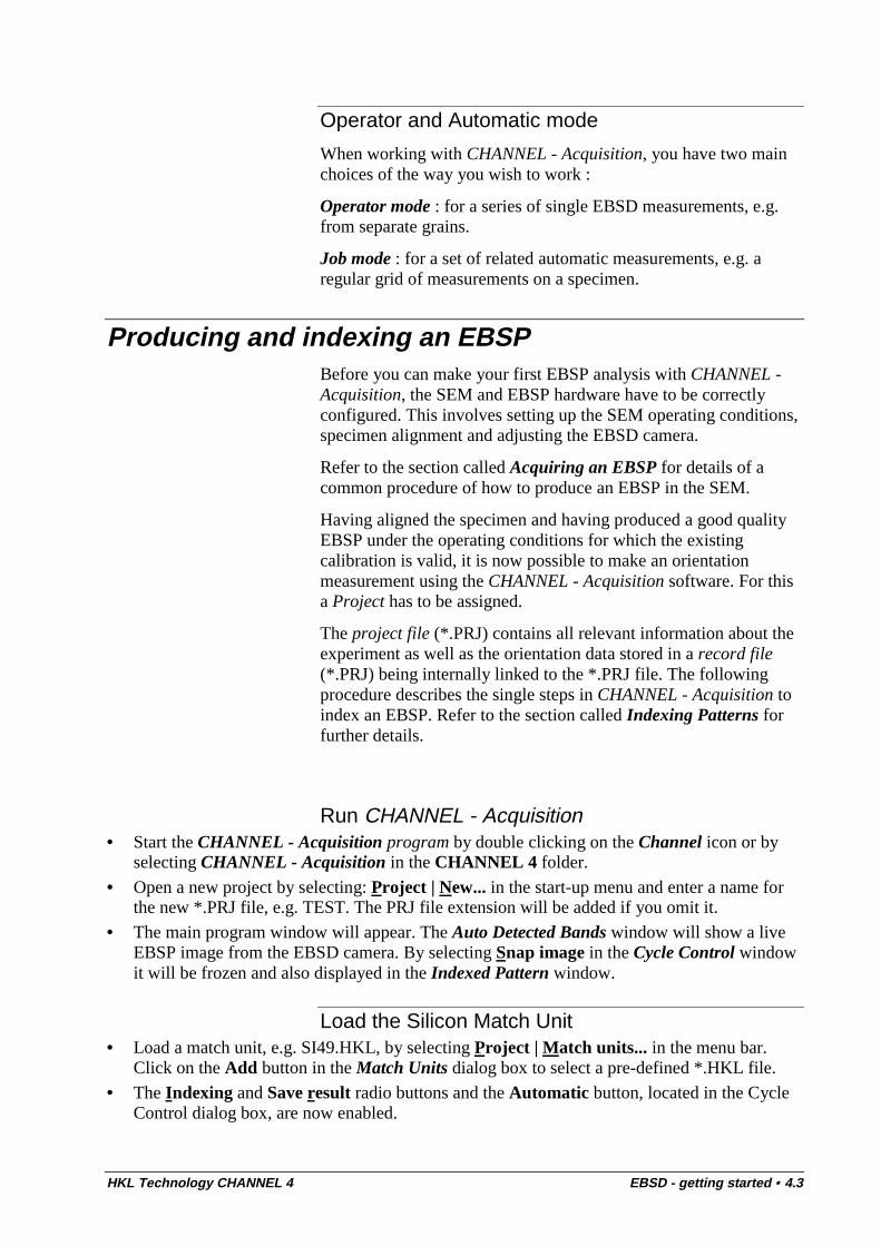
Operator and Automatic mode
When working with CHANNEL - Acquisition, you have two mainchoices of the way you wish to work :
Operator mode : for a series of single EBSD measurements, e.g.from separate grains.
Job mode : for a set of related automatic measurements, e.g. aregular grid of measurements on a specimen.
Producing and indexing an EBSPBefore you can make your first EBSP analysis with CHANNEL -Acquisition, the SEM and EBSP hardware have to be correctlyconfigured. This involves setting up the SEM operating conditions,specimen alignment and adjusting the EBSD camera.
Refer to the section called Acquiring an EBSP for details of acommon procedure of how to produce an EBSP in the SEM.
Having aligned the specimen and having produced a good qualityEBSP under the operating conditions for which the existingcalibration is valid, it is now possible to make an orientationmeasurement using the CHANNEL - Acquisition software. For thisa Project has to be assigned.
The project file (*.PRJ) contains all relevant information about theexperiment as well as the orientation data stored in a record file(*.PRJ) being internally linked to the *.PRJ file. The followingprocedure describes the single steps in CHANNEL - Acquisition toindex an EBSP. Refer to the section called Indexing Patterns forfurther details.
Run CHANNEL - Acquisition• Start the CHANNEL - Acquisition program by double clicking on the Channel icon or by
selecting CHANNEL - Acquisition in the CHANNEL 4 folder.
• Open a new project by selecting: Project | New... in the start-up menu and enter a name forthe new *.PRJ file, e.g. TEST. The PRJ file extension will be added if you omit it.
• The main program window will appear. The Auto Detected Bands window will show a liveEBSP image from the EBSD camera. By selecting Snap image in the Cycle Control windowit will be frozen and also displayed in the Indexed Pattern window.
Load the Silicon Match Unit• Load a match unit, e.g. SI49.HKL, by selecting Project | Match units... in the menu bar.
Click on the Add button in the Match Units dialog box to select a pre-defined *.HKL file.
• The Indexing and Save result radio buttons and the Automatic button, located in the CycleControl dialog box, are now enabled.
4.4 • EBSD - getting started HKL Technology CHANNEL 4
Load a Calibration• Load an EBSD calibration by selecting Calibrate | Load… in the menu bar and choose a
*.CAL file which is valid for the current operating conditions. Or, on first application of theCHANNEL - Acquisition software just use the existing calibration settings alternatively.
Indicate an Area of Interest• Indicate an area of interest (AOI) in your EBSP by selecting Configure | Area of interest
(AOI) . Click on the circle with the Left Mouse Button and drag the circle to a suitable place.You can scale the circle by clicking with the Right Mouse Button and moving the mouse.Close the window (top left icon) to accept the changes.
Configure the SEM conditions• Select Configure | SEM conditions.... and enter the SEM operating conditions (acceleration
voltage, kV, and stage tilt, °)
Detect the Kikuchi Bands in the EBSP• Perform an automatic Kikuchi band detection by clicking on the Detect bands radio button in
the Cycle Control window with the left mouse button.
• The detected Kikuchi bands will be superposed on the actual EBSP in the Auto DetectedBands window. Compare the actual and detected Kikuchi bands and check if they are inagreement. (Refer to the section called Critical choice of reflectors used in the match unitfor more details).
Automatically index the EBSP• Perform an automatic indexing by clicking on the Indexing radio button in the Cycle Control
window with the left mouse button.
Critically assess the EBSP and simulation• A simulation of the EBSP will be superposed on the actual EBSP in the Indexed Pattern
window. Compare the actual and simulated EBSP and see if there is a good match in thepositions of the bands. (N.B. If the software has not managed a valid indexing, then checkthat the match unit(s), calibration or SEM operating conditions are correct).
Save the Data• Save the result by clicking on the Save result radio button in the Cycle Control window.
If an invalid result has accidentally been saved, remove it by pressing the Delete last button.
Repeat with a new EBSP• Select a new grain or part of the specimen, produce and EBSP, index it. Adjust the settings if
necessary and repeat until you are confident that index the majority of the EBSPs examined.
Note: Be careful not to adjust the focus - use the specimen stage Z-control to bring the specimen back into focus, otherwise thecalibration may become invalid.
HKL Technology CHANNEL 4 EBSD - getting started • 4.5
• When you have finished, close the project by selecting Project | Close in the menu bar. Theresults are stored in the *.PRJ file for further processing (see following).
• Exit the Channel program by selecting Project | Exit in the menu bar.
The cycle control window
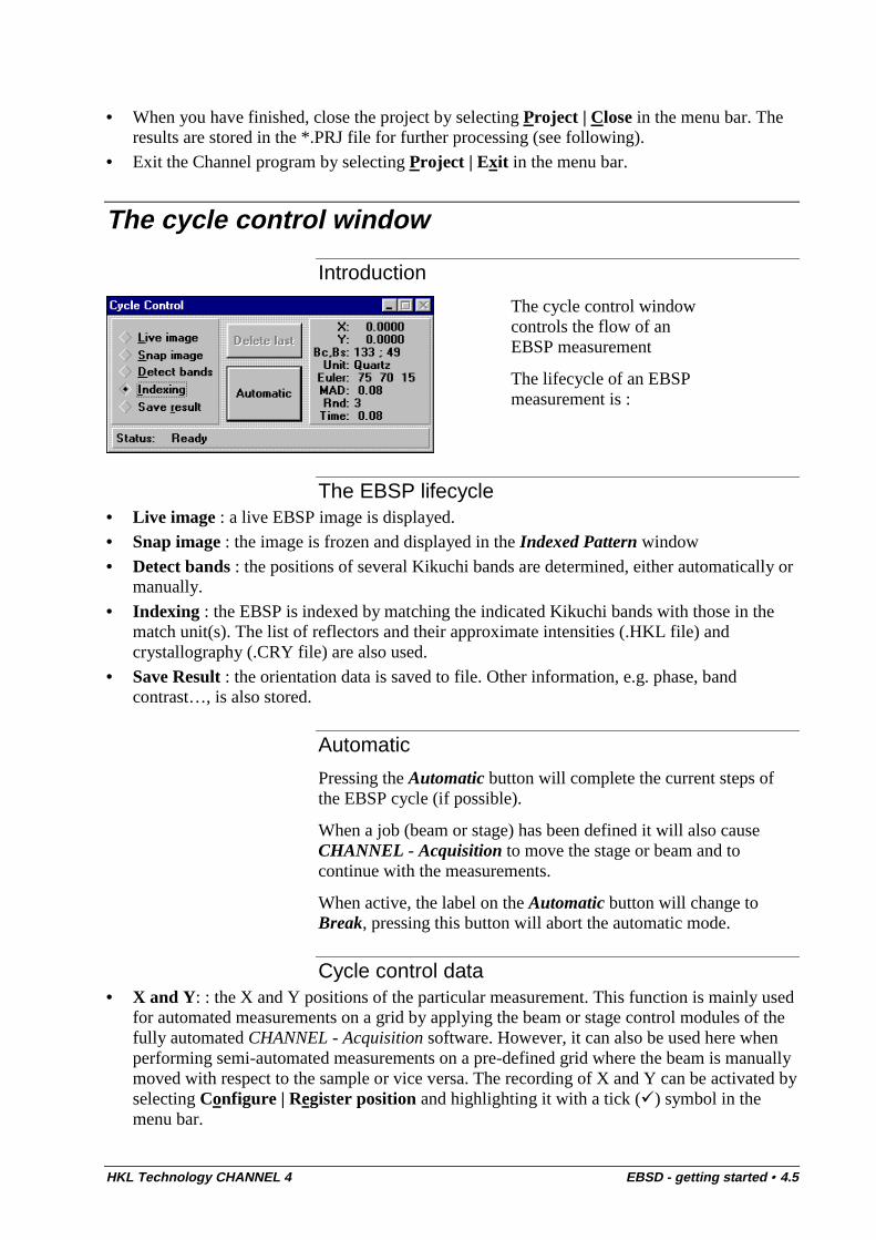
Introduction
The cycle control windowcontrols the flow of anEBSP measurement
The lifecycle of an EBSPmeasurement is :
The EBSP lifecycle• Live image : a live EBSP image is displayed.• Snap image : the image is frozen and displayed in the Indexed Pattern window
• Detect bands : the positions of several Kikuchi bands are determined, either automatically ormanually.
• Indexing : the EBSP is indexed by matching the indicated Kikuchi bands with those in thematch unit(s). The list of reflectors and their approximate intensities (.HKL file) andcrystallography (.CRY file) are also used.
• Save Result : the orientation data is saved to file. Other information, e.g. phase, bandcontrast…, is also stored.
Automatic
Pressing the Automatic button will complete the current steps ofthe EBSP cycle (if possible).
When a job (beam or stage) has been defined it will also causeCHANNEL - Acquisition to move the stage or beam and tocontinue with the measurements.
When active, the label on the Automatic button will change toBreak, pressing this button will abort the automatic mode.
Cycle control data• X and Y: : the X and Y positions of the particular measurement. This function is mainly used
for automated measurements on a grid by applying the beam or stage control modules of thefully automated CHANNEL - Acquisition software. However, it can also be used here whenperforming semi-automated measurements on a pre-defined grid where the beam is manuallymoved with respect to the sample or vice versa. The recording of X and Y can be activated byselecting Configure | Register position and highlighting it with a tick (ä) symbol in themenu bar.

4.6 • EBSD - getting started HKL Technology CHANNEL 4
• Bc, Bs: the values for band contrast and band slope of the measured Kikuchi pattern in abyte range from 0 to 255.
• Unit: the crystal structure, i.e. match unit used for which the indexing procedure produced avalid result.
• Euler: the orientation data given in form of the 3 Euler angles in degrees. See Glossary entry.
• MAD: the mean angular deviation (in degrees), i.e. the average angular misfit between thedetected and indexed Kikuchi bands.
• Rnd: the number of search rounds needed to obtain an indexing solution.
• Time: the time (in seconds) needed to perform the requested procedure in the Cycle Controlwindow. In Automatic mode it refers to the whole cycle.
• Status: the status of a measurement; it shows the following messages:• Busy: when active calculations for band detection and indexing are running• Ready: when finished with the calculations• Indexing not possible: when not having found a valid indexing solution
• Band contrast too low: when not being able to detect Kikuchi bands automatically withinthe limits set as discriminators for the automatic band detection.
• Band slope too low: when not being able to detect the edges of Kikuchi bandsautomatically within the limits set as discriminators for the automatic band detection.
HKL Technology CHANNEL 4 EBSD - getting started • 4.7
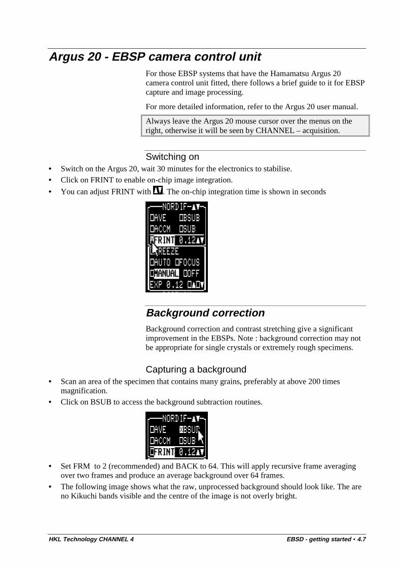
Argus 20 - EBSP camera control unitFor those EBSP systems that have the Hamamatsu Argus 20camera control unit fitted, there follows a brief guide to it for EBSPcapture and image processing.
For more detailed information, refer to the Argus 20 user manual.
Always leave the Argus 20 mouse cursor over the menus on theright, otherwise it will be seen by CHANNEL – acquisition.
Switching on• Switch on the Argus 20, wait 30 minutes for the electronics to stabilise.• Click on FRINT to enable on-chip image integration.
• You can adjust FRINT with . The on-chip integration time is shown in seconds
Background correctionBackground correction and contrast stretching give a significantimprovement in the EBSPs. Note : background correction may notbe appropriate for single crystals or extremely rough specimens.
Capturing a background• Scan an area of the specimen that contains many grains, preferably at above 200 times
magnification.• Click on BSUB to access the background subtraction routines.
• Set FRM to 2 (recommended) and BACK to 64. This will apply recursive frame averagingover two frames and produce an average background over 64 frames.
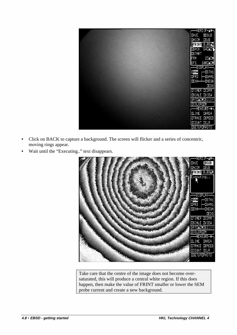
• The following image shows what the raw, unprocessed background should look like. The areno Kikuchi bands visible and the centre of the image is not overly bright.
4.8 • EBSD - getting started HKL Technology CHANNEL 4
• Click on BACK to capture a background. The screen will flicker and a series of concentric,moving rings appear.
• Wait until the “Executing..” text disappears.
Take care that the centre of the image does not become over-saturated, this will produce a central white region. If this doeshappen, then make the value of FRINT smaller or lower the SEMprobe current and create a new background.
HKL Technology CHANNEL 4 EBSD - getting started • 4.9
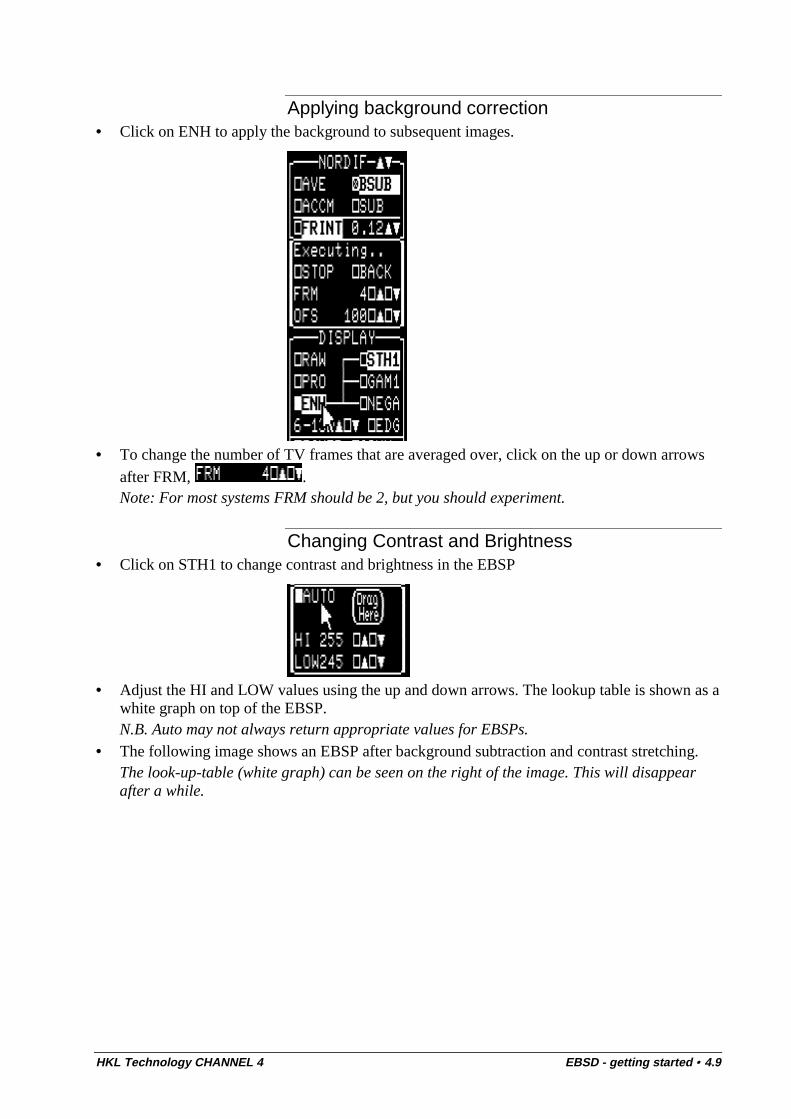
Applying background correction• Click on ENH to apply the background to subsequent images.
• To change the number of TV frames that are averaged over, click on the up or down arrows
after FRM, .Note: For most systems FRM should be 2, but you should experiment.
Changing Contrast and Brightness• Click on STH1 to change contrast and brightness in the EBSP
• Adjust the HI and LOW values using the up and down arrows. The lookup table is shown as awhite graph on top of the EBSP.N.B. Auto may not always return appropriate values for EBSPs.
• The following image shows an EBSP after background subtraction and contrast stretching.The look-up-table (white graph) can be seen on the right of the image. This will disappearafter a while.
4.10 • EBSD - getting started HKL Technology CHANNEL 4
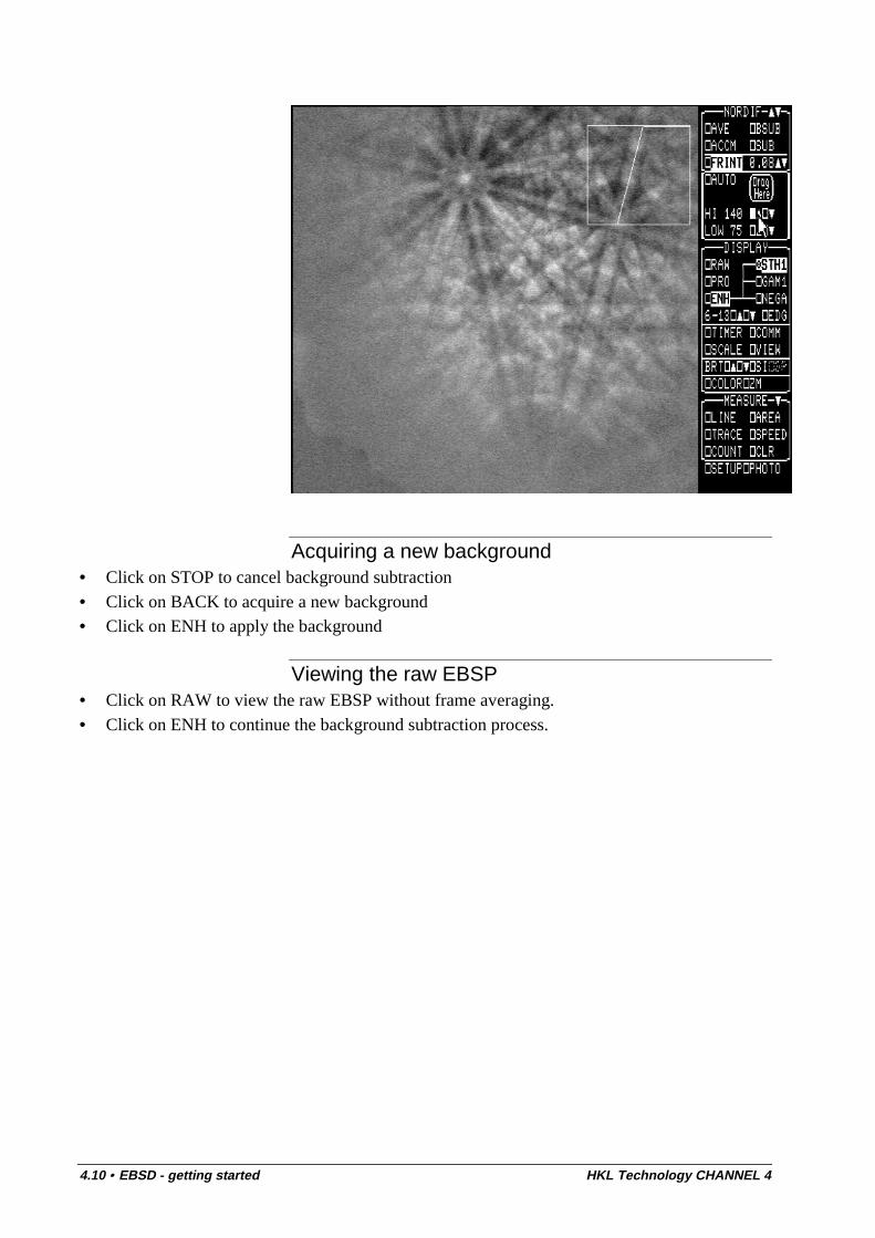
Acquiring a new background• Click on STOP to cancel background subtraction• Click on BACK to acquire a new background• Click on ENH to apply the background
Viewing the raw EBSP• Click on RAW to view the raw EBSP without frame averaging.• Click on ENH to continue the background subtraction process.
HKL Technology CHANNEL 4 EBSD - getting started • 4.11
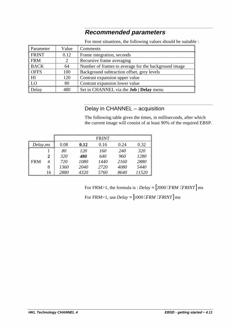
Recommended parametersFor most situations, the following values should be suitable :
Parameter Value CommentsFRINT 0.12 Frame integration, secondsFRM 2 Recursive frame averagingBACK 64 Number of frames to average for the background imageOFFS 100 Background subtraction offset, grey levelsHI 120 Contrast expansion upper valueLO 80 Contrast expansion lower valueDelay 480 Set in CHANNEL via the Job | Delay menu
Delay in CHANNEL – acquisition
The following table gives the times, in milliseconds, after whichthe current image will consist of at least 90% of the required EBSP.
FRINTDelay,ms 0.08 0.12 0.16 0.24 0.32
1 80 120 160 240 3202 320 480 640 960 1280
FRM 4 720 1080 1440 2160 28808 1360 2040 2720 4080 544016 2880 4320 5760 8640 11520
For FRM>1, the formula is : [ ]ms2000 FRINTFRMDelay ⋅⋅≈
For FRM=1, use [ ]ms1000 FRINTFRMDelay ⋅⋅≈
4.12 • EBSD - getting started HKL Technology CHANNEL 4
Stage and Beam Jobs
IntroductionCHANNEL – Acquisition has the ability to take over the beam andstage control of most SEMs and to generate EBSP measurementsfrom a regular grid of points. This allows, orientation maps, forexample, to be produced and is rapidly becoming a new way ofimaging microstructure.
N.B: The Stage and / or Beam hardware and software need to beinstalled and configured by HKL Technology’s representativesbefore these features are available.
General Scanning Instructions• Configure the SEM and EBSP system for manual EBSP analysis. If your SEM has dynamic
focussing facilities then switch them on and focus the tilted specimen.
• It is usually a good idea to save or print an image (secondary electron…) of the region youare looking at.
• Go in to Spot Mode and produce an EBSP. Adjust the probe current and EBSP camera asrequired.
• Move the probe about the selected region and check that the EBSPs are of a reasonablequality. Check that the EBSP background used for background correction is suitable.
Adjusting Delay and Cycle Control Parameters
While a stage or beam job is running, you can press the Breakbutton in the Cycle control window and adjust the Delay and CycleControl parameters.
Press the Automatic button to continue the job.
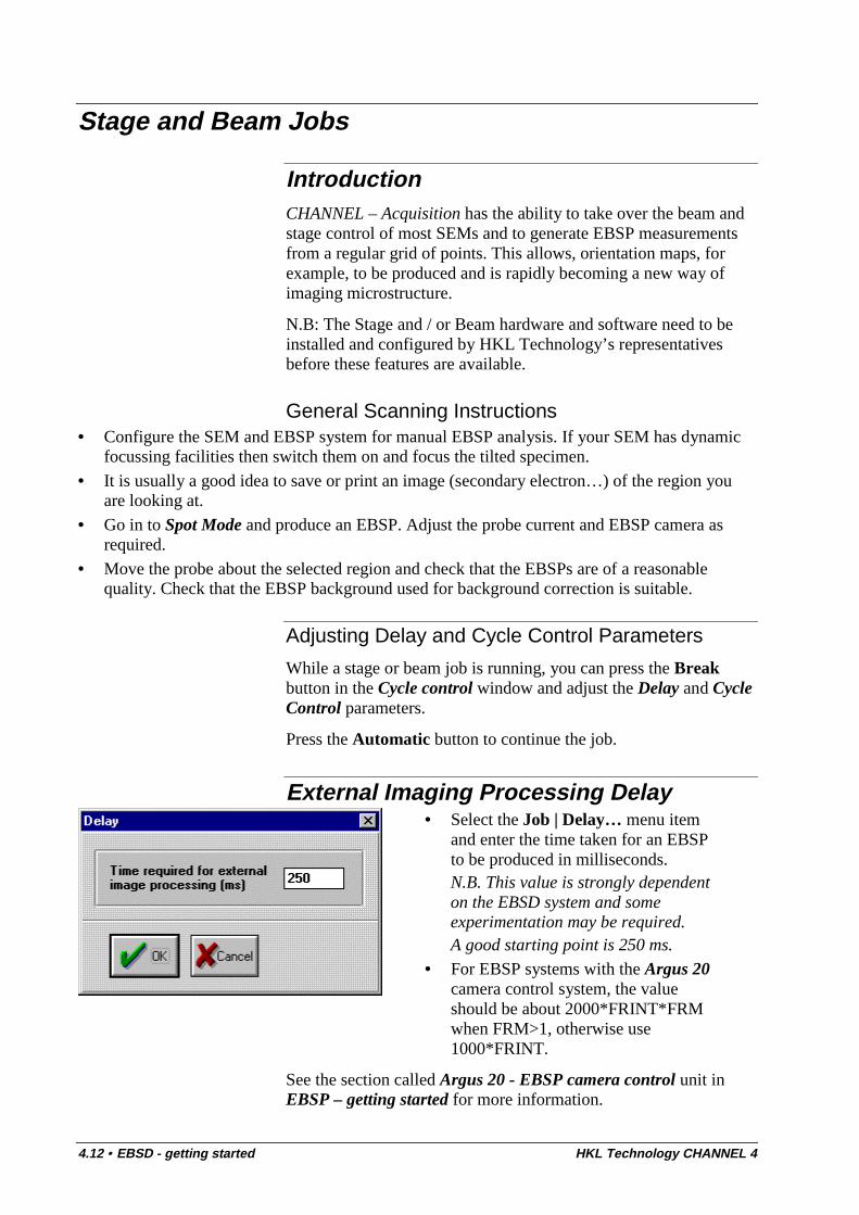
External Imaging Processing Delay• Select the Job | Delay… menu item
and enter the time taken for an EBSPto be produced in milliseconds.N.B. This value is strongly dependenton the EBSD system and someexperimentation may be required.A good starting point is 250 ms.
• For EBSP systems with the Argus 20camera control system, the valueshould be about 2000*FRINT*FRMwhen FRM>1, otherwise use1000*FRINT.
See the section called Argus 20 - EBSP camera control unit inEBSP – getting started for more information.

HKL Technology CHANNEL 4 EBSD - getting started • 4.13
4.14 • EBSD - getting started HKL Technology CHANNEL 4
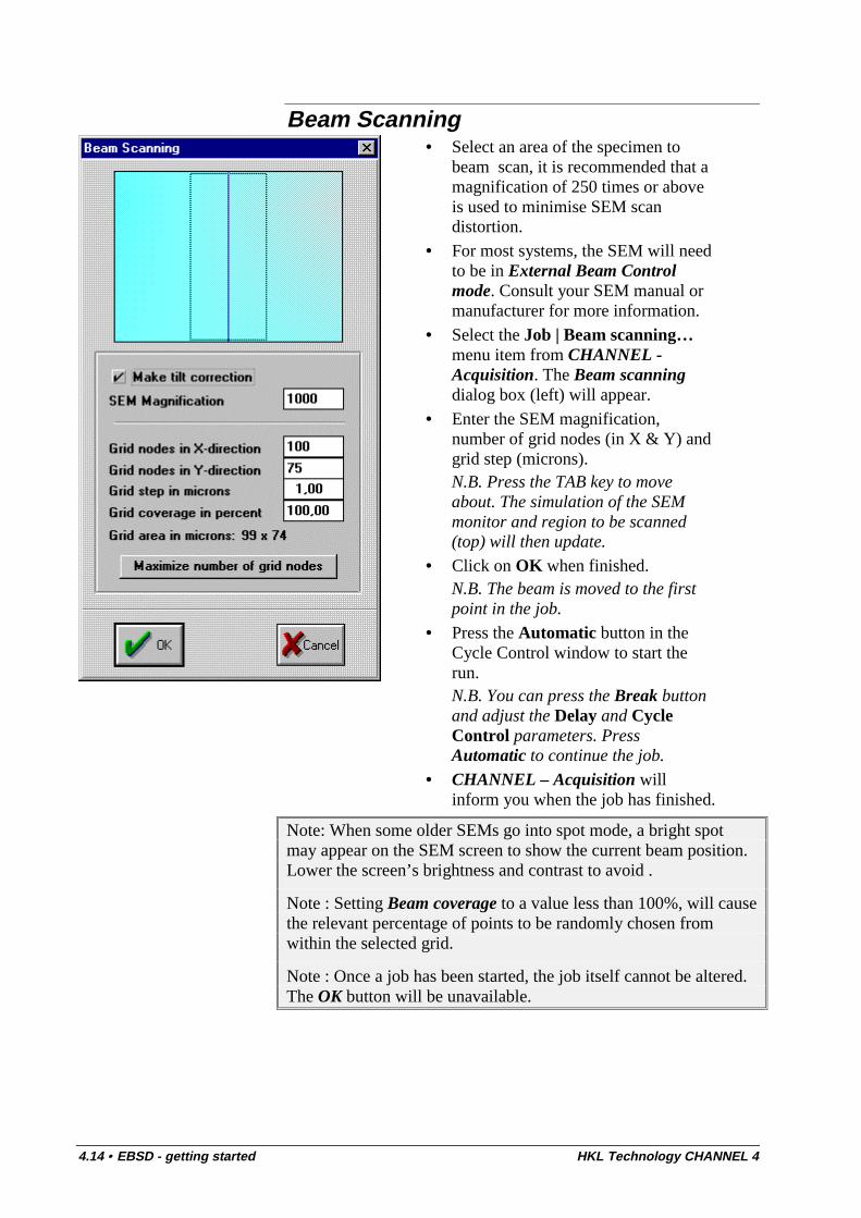
Beam Scanning• Select an area of the specimen to
beam scan, it is recommended that amagnification of 250 times or aboveis used to minimise SEM scandistortion.
• For most systems, the SEM will needto be in External Beam Controlmode. Consult your SEM manual ormanufacturer for more information.
• Select the Job | Beam scanning…menu item from CHANNEL -Acquisition. The Beam scanningdialog box (left) will appear.
• Enter the SEM magnification,number of grid nodes (in X & Y) andgrid step (microns).N.B. Press the TAB key to moveabout. The simulation of the SEMmonitor and region to be scanned(top) will then update.
• Click on OK when finished.N.B. The beam is moved to the firstpoint in the job.
• Press the Automatic button in theCycle Control window to start therun.N.B. You can press the Break buttonand adjust the Delay and CycleControl parameters. PressAutomatic to continue the job.
• CHANNEL – Acquisition willinform you when the job has finished.
Note: When some older SEMs go into spot mode, a bright spotmay appear on the SEM screen to show the current beam position.Lower the screen’s brightness and contrast to avoid .
Note : Setting Beam coverage to a value less than 100%, will causethe relevant percentage of points to be randomly chosen fromwithin the selected grid.
Note : Once a job has been started, the job itself cannot be altered.The OK button will be unavailable.
HKL Technology CHANNEL 4 EBSD - getting started • 4.15
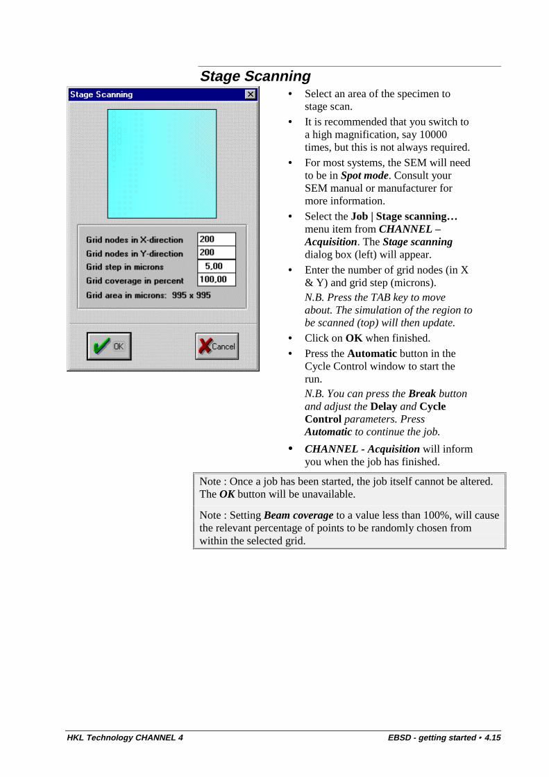
Stage Scanning• Select an area of the specimen to
stage scan.• It is recommended that you switch to
a high magnification, say 10000times, but this is not always required.
• For most systems, the SEM will needto be in Spot mode. Consult yourSEM manual or manufacturer formore information.
• Select the Job | Stage scanning…menu item from CHANNEL –Acquisition. The Stage scanningdialog box (left) will appear.
• Enter the number of grid nodes (in X& Y) and grid step (microns).N.B. Press the TAB key to moveabout. The simulation of the region tobe scanned (top) will then update.
• Click on OK when finished.• Press the Automatic button in the
Cycle Control window to start therun.N.B. You can press the Break buttonand adjust the Delay and CycleControl parameters. PressAutomatic to continue the job.
• CHANNEL - Acquisition will informyou when the job has finished.
Note : Once a job has been started, the job itself cannot be altered.The OK button will be unavailable.
Note : Setting Beam coverage to a value less than 100%, will causethe relevant percentage of points to be randomly chosen fromwithin the selected grid.

HKL Technology CHANNEL 4 EBSD system calibration • 5.1
EBSD system calibration
IntroductionThe calibration of an EBSP system is probably the most importantoperation to perform, since poor calibration leads to unreliableabsolute (i.e. crystal to sample) orientation measurements. Carefulcalibration should therefore become a routine procedure.
An initial calibration of the system will be carried out when it isinstalled.
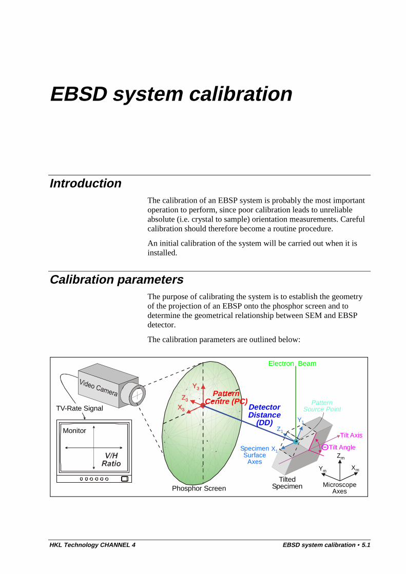
Calibration parametersThe purpose of calibrating the system is to establish the geometryof the projection of an EBSP onto the phosphor screen and todetermine the geometrical relationship between SEM and EBSPdetector.
The calibration parameters are outlined below:
Z1
Y1
X1
TiltedSpecimen
Electron Beam
SpecimenSurface
Axes
Tilt Axis
Tilt Angle
XmYm
Zm
MicroscopeAxes
Θ
Phosphor Screen
PatternSource Point
Monitor
TV-Rate Signal
PatternCentre (PC)
Detector Distance
(DD)
5.2 • EBSD system calibration HKL Technology CHANNEL 4
Pattern Centre• The pattern centre (PC): the point on the imaging phosphor/detector closest to the pattern
source point, i.e. its projection perpendicular from the phosphor screen. The value isexpressed in x- and y- co-ordinates (PCx / PCy), with (0,0 / 0,0) being at the bottom left ofthe screen. The PC is measured in pattern units. Typical values are PCx=0,5 and PCy=0,7(i.e. with a pattern centre approximately 20° above the centre of the imaged EBSP).N.B. All lengths in CHANNEL - Acquisition are measured in pattern units, with 1 unitbeing defined as the width of the captured EBSP image.
Detector Distance• The detector distance (DD): the distance between the specimen and the imaging
phosphor/detector. This is initially calculated by measuring the distance between two knownEBSP zone axes, and relating this back to the known angle between them. The DD ismeasured in pattern units. A typical value is 0,5 (i.e. half the diameter of the EBSP screen);
V/H Ratio• The V/H ratio: the ratio of vertical height to horizontal width of the captured EBSP image on
the screen. The V/H-ratio of a standard TV signal is 0,75;
EBSP camera/detector
Microscope
Tilt axis
X1
Y1
Z1 Sample
Electron beam
X3
Y3
Z3XmYm
Zm
Csm
SEM
’Detector Orientation’
Detector
Cs3
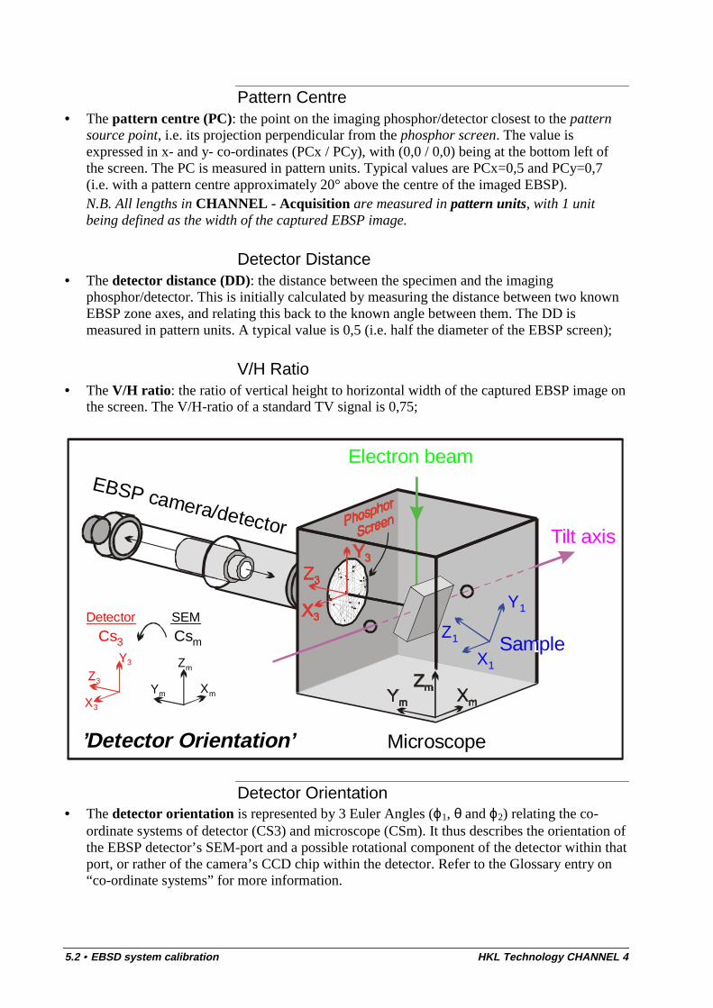
Detector Orientation• The detector orientation is represented by 3 Euler Angles (ϕ1, θ and ϕ2) relating the co-
ordinate systems of detector (CS3) and microscope (CSm). It thus describes the orientation ofthe EBSP detector’s SEM-port and a possible rotational component of the detector within thatport, or rather of the camera’s CCD chip within the detector. Refer to the Glossary entry on“co-ordinate systems” for more information.
HKL Technology CHANNEL 4 EBSD system calibration • 5.3
Note : In CHANNEL - Acquisition the detector orientation alsocompensates for systematic errors resulting from inaccuracies inthe stage tilt and pattern centre. It thus does not represent anabsolute figure for your system and will have to be refined whenoperating conditions (i.e. stage tilt, working distance etc.) arechanged!
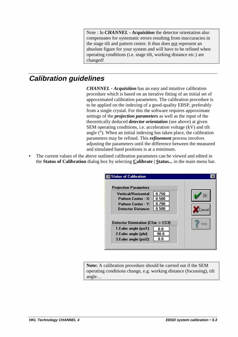
Calibration guidelinesCHANNEL - Acquisition has an easy and intuitive calibrationprocedure which is based on an iterative fitting of an initial set ofapproximated calibration parameters. The calibration procedure isto be applied on the indexing of a good-quality EBSP, preferablyfrom a single crystal. For this the software requires approximatesettings of the projection parameters as well as the input of thetheoretically deduced detector orientation (see above) at givenSEM operating conditions, i.e. acceleration voltage (kV) and tiltangle (°). When an initial indexing has taken place, the calibrationparameters may be refined. This refinement process involvesadjusting the parameters until the difference between the measuredand simulated band positions is at a minimum.
• The current values of the above outlined calibration parameters can be viewed and edited inthe Status of Calibration dialog box by selecting Calibrate | Status... in the main menu bar.
Note: A calibration procedure should be carried out if the SEMoperating conditions change, e.g. working distance (focussing), tiltangle…
5.4 • EBSD system calibration HKL Technology CHANNEL 4
Silicon as a Calibrant
It is strongly recommended that all calibrations are carried outusing a single crystal. The commonest calibration method usespiece of a single crystal silicon wafer (e.g. with surface normal(001) and a [110] type reference direction) as a standard specimenof known orientation from which the projection parameters as wellas the detector orientation can be derived with the help ofCHANNEL - Acquisition.
Guidelines for the use of Silicon• Use as large a piece of silicon as is practical,
• If possible, mount the silicon directly onto your specimen, or use a specimen holder that has apiece of silicon firmly attached to it,
• By eye, make sure that the cleaved edge of the silicon is horizontal,• Make sure that the silicon is inclined (typically at 70°) from the horizontal.
Accurately align the Silicon cleaved edge
If your SEM has the facility to rotate the silicon about its surfacenormal then the following procedure should be used to accuratelyalign the cleaved edge.
• Zoom-in on the cleaved edge of the silicon specimen,
• Using only the stage movement along the tilt axis, track along the cleaved edge of the siliconand watch to see if it moves away from a fixed point on the SEM monitor.
• If the cleaved edge moves then the silicon is not properly aligned and will need to be rotated.In this case, rotate the silicon by a few degrees and repeat the above procedure, until the edgestays in a fixed position all the time.
• It is sometimes useful to start at a low magnification, align the silicon, and then move to ahigher one.
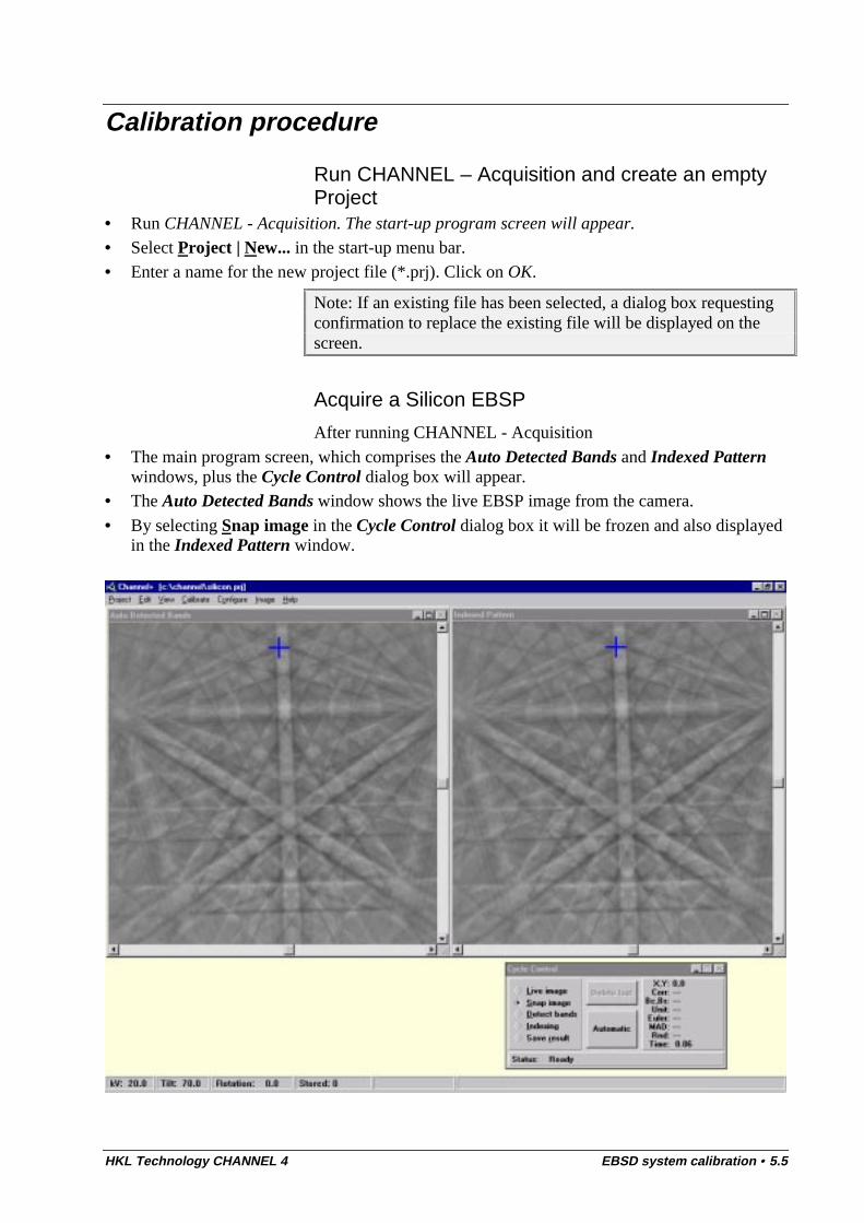
HKL Technology CHANNEL 4 EBSD system calibration • 5.5
Calibration procedure
Run CHANNEL – Acquisition and create an emptyProject
• Run CHANNEL - Acquisition. The start-up program screen will appear.
• Select Project | New... in the start-up menu bar.• Enter a name for the new project file (*.prj). Click on OK.
Note: If an existing file has been selected, a dialog box requestingconfirmation to replace the existing file will be displayed on thescreen.
Acquire a Silicon EBSP
After running CHANNEL - Acquisition
• The main program screen, which comprises the Auto Detected Bands and Indexed Patternwindows, plus the Cycle Control dialog box will appear.
• The Auto Detected Bands window shows the live EBSP image from the camera.
• By selecting Snap image in the Cycle Control dialog box it will be frozen and also displayedin the Indexed Pattern window.
5.6 • EBSD system calibration HKL Technology CHANNEL 4
Load Silicon match unit• Load a match unit by selecting Project | Match units... in the menu bar. The Match Units
dialog box will appear on screen. Click on the Add button to reveal the Load Match Unitdialog box. The match unit files (*.HKL) contain the crystal structure as a set of reflectorsand inter-planar angles which are needed to index a given EBSP.
• Select SI49.HKL, from the list and click on OK. N.B. Change directory if necessary.
• Click on OK. The Indexing and Save result radio buttons and the Automatic button in theCycle Control window are now enabled.
Configure SEM conditions• Select Configure | SEM conditions.... and enter the SEM operating conditions (acceleration
voltage, kV, and stage tilt, °).
Mark approximate Pattern Centre• Set an approximate pattern centre (PC) by selecting Calibrate | Approx Settings | Pattern
Centre in the menu bar. The Identify the Pattern Centre window will appear on the screen.It will show the actual EBSP image, a blue cross (the old PC) and a moveable white crosslabelled PC (the cursor for the new PC).
Note: You can establish an approximate PC by carefully movingthe phosphor screen in and out. This creates a zooming effect onthe actual EBSP image. The PC is the part of the image whichappears stationary.
• Move the cursor to where you want the new PC to be and click the left mouse button. A bluecross will signify the new PC in the Auto Detected Bands window.
Setting the approximate Detector Distance• Set an approximate detector distance (DD) by selecting Calibrate | Approx. Settings |
Detector Distance in the menu bar.The Approximate Setting of Detector Distance window will appear on the screen. It willshow the actual EBSP image, the match unit selected for indexing, two fields for the input oftwo different zone axes and two fields where the current and new DD are displayed. You needto tell CHANNEL - Acquisition where two crystallographic zones are positioned, from thisCHANNEL - Acquisition can calculate DD.
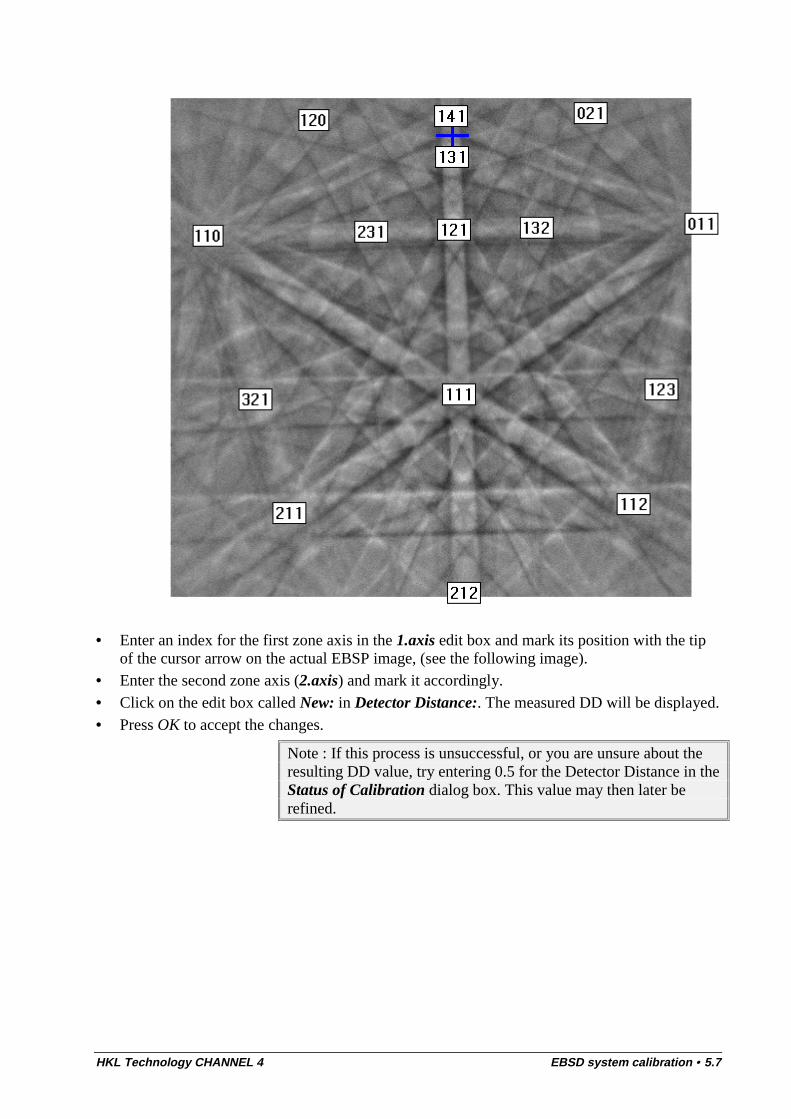
HKL Technology CHANNEL 4 EBSD system calibration • 5.7
• Enter an index for the first zone axis in the 1.axis edit box and mark its position with the tipof the cursor arrow on the actual EBSP image, (see the following image).
• Enter the second zone axis (2.axis) and mark it accordingly.• Click on the edit box called New: in Detector Distance:. The measured DD will be displayed.• Press OK to accept the changes.
Note : If this process is unsuccessful, or you are unsure about theresulting DD value, try entering 0.5 for the Detector Distance in theStatus of Calibration dialog box. This value may then later berefined.
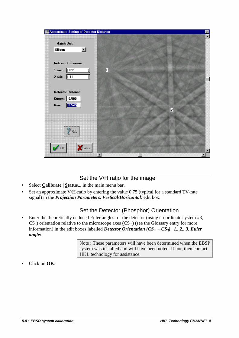
5.8 • EBSD system calibration HKL Technology CHANNEL 4
Set the V/H ratio for the image• Select Calibrate | Status... in the main menu bar.
• Set an approximate V/H-ratio by entering the value 0.75 (typical for a standard TV-ratesignal) in the Projection Parameters, Vertical/Horizontal: edit box.
Set the Detector (Phosphor) Orientation• Enter the theoretically deduced Euler angles for the detector (using co-ordinate system #3,
CS3) orientation relative to the microscope axes (CSm) (see the Glossary entry for moreinformation) in the edit boxes labelled Detector Orientation (CSm→CS3) | 1., 2., 3. Eulerangle:.
Note : These parameters will have been determined when the EBSPsystem was installed and will have been noted. If not, then contactHKL technology for assistance.
• Click on OK.
HKL Technology CHANNEL 4 EBSD system calibration • 5.9
Calibration refinements
Introduction
After the above described establishment of approximate calibrationparameters has been carried out, it will be necessary to refine theseparameters, based on the indexing of a live EBSP image of thesilicon; this procedure is described below:
Note: Accurate detection of the Kikuchi,bands is essential foreffective calibration. Therefore when undertaking a calibrationrefinement, detect the Kikuchi bands manually and with care.
Detect the Kikuchi Bands manually• Follow the instructions given in the section called “Manually detecting bands” and mark the
positions of about 6 Kikuchi bands. Try to make them evenly spaced apart across the EBSP.
Indexing the calibration specimen EBSP• Click on Indexing in the Cycle Control window and compare the simulated EBSP on the
right with the original EBSP on the left. If there is a good match then proceed to the next step,if not repeat the earlier steps for setting approximate calibration parameters (PC, DD…) untila good match is achieved.The Mean Angular Deviation (MAD) shown on the right of the Cycle Control window is ameasure of how well positions of the bands in the simulated EBSP match those in the actualEBSP. The smaller the number the better the match, 0.5 to 2° is usual at this stage.
Refining the calibration parameters
The approximate calibration parameters can now be refined to givea more accurate and reliable calibration.
• You can refine the projection parameters and reduce the MAD number by selectingCalibrate | Refinements | Projection Parameters....
• The Refine Projection Parameters dialog box will appear on screen.• Under Projection Parameters:, ensure the VH, PC and DD boxes have a tick (ä).• Click on OK to accept the new values.• Check that the MAD number in the Cycle Control dialog box has become smaller.
Repeat the previous 5 steps until the MAD number remains constant.
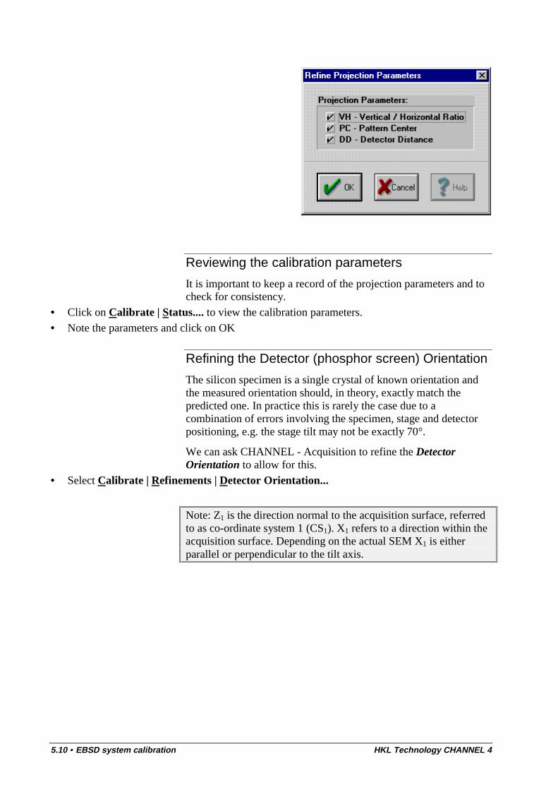
5.10 • EBSD system calibration HKL Technology CHANNEL 4
Reviewing the calibration parameters
It is important to keep a record of the projection parameters and tocheck for consistency.
• Click on Calibrate | Status.... to view the calibration parameters.• Note the parameters and click on OK
Refining the Detector (phosphor screen) Orientation
The silicon specimen is a single crystal of known orientation andthe measured orientation should, in theory, exactly match thepredicted one. In practice this is rarely the case due to acombination of errors involving the specimen, stage and detectorpositioning, e.g. the stage tilt may not be exactly 70°.
We can ask CHANNEL - Acquisition to refine the DetectorOrientation to allow for this.
• Select Calibrate | Refinements | Detector Orientation...
Note: Z1 is the direction normal to the acquisition surface, referredto as co-ordinate system 1 (CS1). X1 refers to a direction within theacquisition surface. Depending on the actual SEM X1 is eitherparallel or perpendicular to the tilt axis.
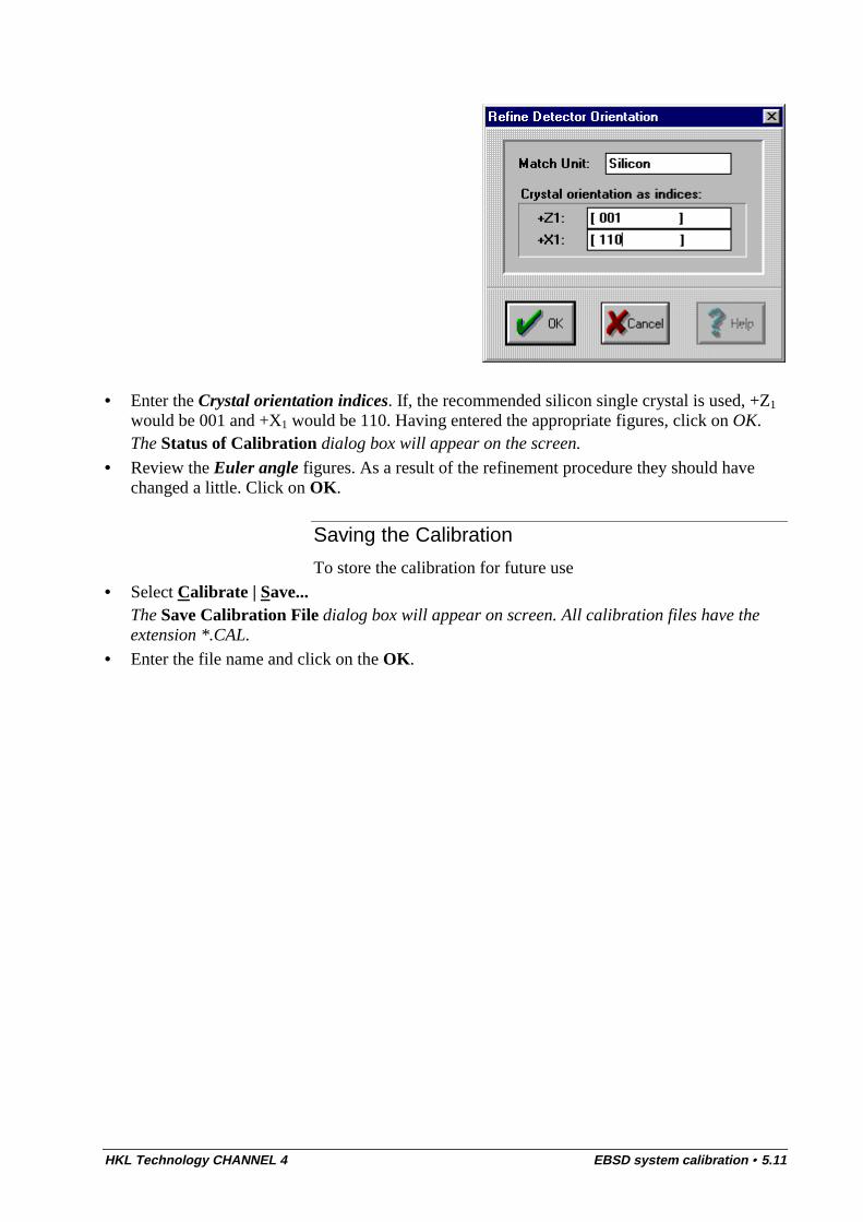
HKL Technology CHANNEL 4 EBSD system calibration • 5.11
• Enter the Crystal orientation indices. If, the recommended silicon single crystal is used, +Z1
would be 001 and +X1 would be 110. Having entered the appropriate figures, click on OK.The Status of Calibration dialog box will appear on the screen.
• Review the Euler angle figures. As a result of the refinement procedure they should havechanged a little. Click on OK.
Saving the Calibration
To store the calibration for future use• Select Calibrate | Save...
The Save Calibration File dialog box will appear on screen. All calibration files have theextension *.CAL.
• Enter the file name and click on the OK.

HKL Technology CHANNEL 4 EBSD crystallography • 6.1
EBSD crystallography
Defining a crystal structure
Introduction
To facilitate crystallographic indexing and simulations of EBSPs inCHANNEL - Acquisition, the software requires the input of basiccrystallographic data of the particular crystal structures in theinvestigated material. The program Crystal enables the user tocreate and edit these crystal files (*.CRY) which are the data basefor the generation of match units or reflector files(*.HKL) used inthe indexing procedure in the main program CHANNEL -Acquisition. A match unit is a list of the most diffracting planes(reflectors) in an EBSP (Kikuchi bands) for a particular crystalstructure.
The *.CRY and *.HKL files are usually stored in one of thefollowing directories, either “Channel\Common” or“Program Files\HKL Technology\CHANNEL 4\Common”.
Note: It is good practice to keep a record, in a notebook, of all the*.cry and *.hkl files that are created. This will allow other users touse them with confidence.
6.2 • EBSD crystallography HKL Technology CHANNEL 4
Defining a crystal structure
The program Crystal enables the user to define a crystal structureby creating and editing a crystal file (*.CRY). Although aconsiderable number of *.CRY files is delivered with yourCHANNEL - Acquisition software, it might be necessary to createnew *.CRY files with respect to some specific materialsinvestigated. The relevant crystallographic data can be acquiredfrom many standard references, the main ones are referenced in theBibliography. The information required to define a crystal structuredata is as follows.
Name(structure)
The name of the crystal structure, e.g. Aluminium, a maximum of12 characters are allowed. This name will appear on data of polefigures, etc..
Laue group
The Laue group reflects the symmetry of a crystal with respect toelectron (or X-ray) diffraction. The following table describes thesymmetries that must be present for the various crystal systems.For tetragonal, trigonal, hexagonal & cubic crystals there is achoice between a higher and a lower symmetry version. Bycarefully considering the symmetries in your crystal it should bepossible to decide which of the Laue group symmetry it has.
Pseudosymmetry axis
A pseudosymmetry occurs where two orientations cannot easily bedistinguished due to an apparent n-fold rotation axis in lowersymmetry crystal structures. For example an orthorhombicstructure with similar lengths of the a- and b-axis appears to betetragonal when viewed down its c-axis - this is the case in somehigh temperature superconductors. Other examples ofpseudosymmetry are often encountered in geological materials (e.g.pseudohexagonal structures appearing in trigonal quartz).
CHANNEL - Acquisition has a facility whereby the EBSPsimulation can be rotated about the pseudosymmetry axis by a pre-set angle to allow the operator to select the correct simulation bycomparing the ambiguous solutions with the actual EBSP. To allowthis option the Indices and the n-fold symmetry of the Pseudosymmetry axis have to be defined.
Unit cell parameters
The unit cell parameters define the size and shape of the unit cell.The lengths of the base vectors: a, b and c are measured inÅngström, the interaxial angles: alpha, beta and gamma in degrees.
HKL Technology CHANNEL 4 EBSD crystallography • 6.3
Reference
The original source of the data - this is useful for keeping track ofhow up-to-date data is and will allow other users to use the datawith confidence.
Atoms present in the Unit Cell
To enable EBSP simulations in CHANNEL - Acquisition, which arebased upon structure factor calculations (see the Glossary entry formore details), the software requires the input of all atoms withinthe unit cell of the investigated material.
This can be done by using the editor in the lower part of the Crystalwindow. It includes a scroll box for the list of atom positions (atomtype, unit cell co-ordinates, site occupancy) as well as editablescroll and input boxes to edit and add the single atom positions byactivating the Add, Modify or Delete buttons.
The atom parameters are as follows:
• Atom: to define the type of atom by selecting it from a drop-down list. The following tablefeatures the list of atom types provided in CHANNEL - Acquisition:
• x, y, z (unit cell co-ordinates): to define the [x, y, z] unit cell co-ordinates of the atom asfractions of the unit cell’s a, b and c base vectors. For example [0, 0, 0] is the origin, [1, 1, 1]the diametrically opposite corner and [0.5, 0.5, 0] an atom at the centre of a face.
• Amount (site occupancy): the site occupancy represents how often, on average, a site isoccupied by a particular atom. This number can be between 0 and 1. If an atom is the soleoccupant of a particular site then enter 1, if it shares it equally with another atom then enter0.5 for both atoms.
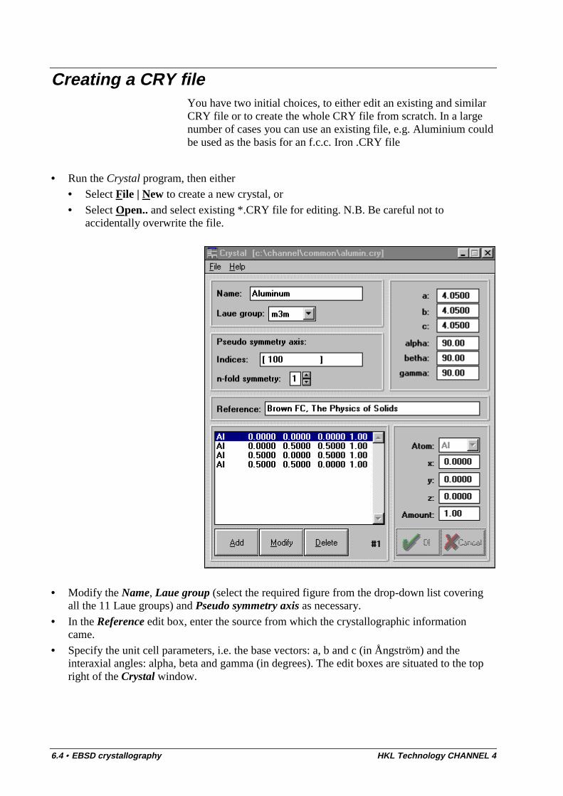
6.4 • EBSD crystallography HKL Technology CHANNEL 4
Creating a CRY fileYou have two initial choices, to either edit an existing and similarCRY file or to create the whole CRY file from scratch. In a largenumber of cases you can use an existing file, e.g. Aluminium couldbe used as the basis for an f.c.c. Iron .CRY file
• Run the Crystal program, then either• Select File | New to create a new crystal, or
• Select Open.. and select existing *.CRY file for editing. N.B. Be careful not toaccidentally overwrite the file.
• Modify the Name, Laue group (select the required figure from the drop-down list coveringall the 11 Laue groups) and Pseudo symmetry axis as necessary.
• In the Reference edit box, enter the source from which the crystallographic informationcame.
• Specify the unit cell parameters, i.e. the base vectors: a, b and c (in Ångström) and theinteraxial angles: alpha, beta and gamma (in degrees). The edit boxes are situated to the topright of the Crystal window.
HKL Technology CHANNEL 4 EBSD crystallography • 6.5
Creating a list of Atom information
You must also create or edit a list of all the atoms within the unitcell of the investigated material done. This is done using the editorin the lower part of the Crystal window. You can move to the scrollbox containing the list of atom positions (atom type, unit cell co-ordinates, site occupancy) with either the mouse or the Tab key.
• To add to or edit the atom information in the list, press either the Add, Modify atom button.After clicking the button, the list and atom edit boxes to the right become enabled. Enter thedata for that atom and press OK.
Note the Atom: list box contains atoms (and ions) arranged byatomic number, e.g. H He Li Be… You can find a particular atomby clicking on the list box and typing the first letter of the atoms’symbol, e.g. “F” for Fe (Iron). Repeat until you reach the atom youwant.
• To delete an atom from the atom list, highlight the atom in the list on the left and click on theDelete button.
• Repeat for all the other atoms in your unit cell.
Save the Crystal Structure to File• Select the File | Save as.. menu item.• Enter a filename and press OK.
Exiting from CRYSTAL• Select File | Exit• If a modified or newly created *.CRY file has not been stored already, you will be asked if
you wish to save the changes.
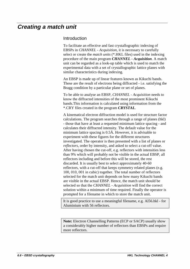
6.6 • EBSD crystallography HKL Technology CHANNEL 4
Creating a match unit
Introduction
To facilitate an effective and fast crystallographic indexing ofEBSPs in CHANNEL - Acquisition, it is necessary to carefullyselect or create the match units (*.HKL files) used in the indexingprocedure of the main program CHANNEL - Acquisition. A matchunit can be regarded as a look-up table which is used to match theexperimental data with a set of crystallographic lattice planes withsimilar characteristics during indexing.
An EBSP is made up of linear features known as Kikuchi bands.These are the result of electrons being diffracted - i.e. satisfying theBragg condition by a particular plane or set of planes.
To be able to analyse an EBSP, CHANNEL - Acquisition needs toknow the diffracted intensities of the most prominent Kikuchibands.This information is calculated using information from the*.CRY files created in the program CRYSTAL.
A kinematical electron diffraction model is used for structure factorcalculations. The program searches through a range of planes (hkl)- those that have at least a requested minimum lattice spacing - andcalculates their diffracted intensity. The default value for theminimum lattice spacing is 0.5Å. However, it is advisable toexperiment with these figures for the different structuresinvestigated. The operator is then presented with a list of planes orreflectors, order by intensity, and asked to select a cut-off value.After having chosen the cut-off, e.g. reflectors with intensities lessthan 9% which will probably not be visible in the actual EBSP, allreflectors including and before this will be stored, the restdiscarded. It is usually best to select approximately 40-60reflectors, with a cut-off that keeps symmetry related planes (e.g.100, 010, 001 in cubic) together. The total number of reflectorsselected for the match unit depends on how many Kikuchi bandsare visible in the actual EBSP. Hence, the match unit should beselected so that the CHANNEL - Acquisition will find the correctsolution within a minimum of time required. Finally the operator isprompted for a filename in which to store the match unit.
It is good practice to use a meaningful filename, e.g. Al56.hkl - forAluminium with 56 reflectors.
Note: Electron Channelling Patterns (ECP or SACP) usually showa considerably higher number of reflectors than EBSPs and requiremore reflectors.
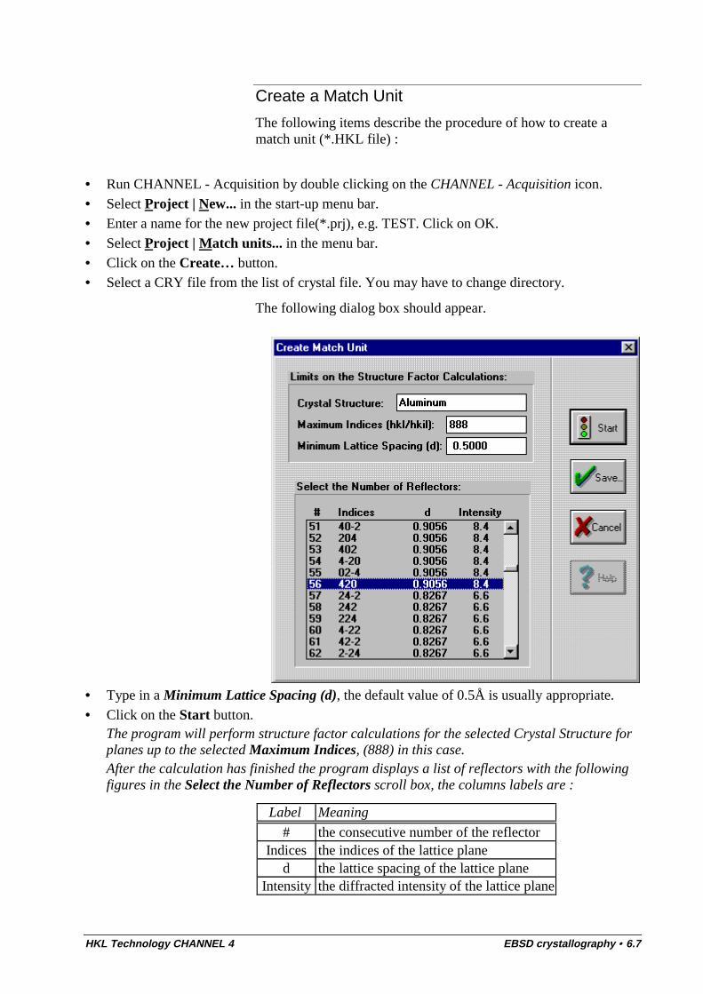
HKL Technology CHANNEL 4 EBSD crystallography • 6.7
Create a Match Unit
The following items describe the procedure of how to create amatch unit (*.HKL file) :
• Run CHANNEL - Acquisition by double clicking on the CHANNEL - Acquisition icon.• Select Project | New... in the start-up menu bar.• Enter a name for the new project file(*.prj), e.g. TEST. Click on OK.• Select Project | Match units... in the menu bar.• Click on the Create… button.• Select a CRY file from the list of crystal file. You may have to change directory.
The following dialog box should appear.
• Type in a Minimum Lattice Spacing (d), the default value of 0.5Å is usually appropriate.• Click on the Start button.
The program will perform structure factor calculations for the selected Crystal Structure forplanes up to the selected Maximum Indices, (888) in this case.After the calculation has finished the program displays a list of reflectors with the followingfigures in the Select the Number of Reflectors scroll box, the columns labels are :
Label Meaning
# the consecutive number of the reflectorIndices the indices of the lattice plane
d the lattice spacing of the lattice planeIntensity the diffracted intensity of the lattice plane
6.8 • EBSD crystallography HKL Technology CHANNEL 4
CHANNEL - Acquisition now needs to know how many reflectorsto use.
• Select a cut-off value by scrolling down the list of reflectors to a number typically between40 and 60 using the scroll bar. Find a reasonable cut-off value, e.g. a reflector with anintensity of less than 9%. Click on this entry in the list, always choosing the last from a set ofsymmetry related reflectors. The selection will be highlighted in blue.
• Click on Save… and save the match unit to an *.HKL file. Choose a meaningful name,Al56.HKL for Aluminium with 56 reflectors, and press OK
• Press the CANCEL button in the Create Match Unit window.
Critical choice of reflectors used in the match unit
Introduction
To achieve an optimum in accuracy and speed for the indexingprocedure in CHANNEL - Acquisition, it is necessary to criticallychoose the number of reflectors used in the match unit with regardto the appearance and quality of the acquired EBSPs. This isdependent on many parameters like material, surface quality, SEMoperating conditions, performance of EBSP detector unit etc..Therefore, the selected match unit(s) have to be reviewed bycomparing the actual EBSPs and the indexing/simulationscarefully. The operator should ask himself the following questions:
• Are all Kikuchi bands to be observed in the actual EBSP also present in the simulation (andthus, will the further indexing procedure perform correctly with the number of reflectors usedin the match unit?)
• Are all Kikuchi bands to be observed in the simulation also present in the actual EBSP? (andhence, will the indexing procedure not be slowed down too much by searching through a longlist of reflectors in the match unit, which contain more information than is required, i.e.present in the actual EBSP image?)
• Is the intensity, i.e. contrast of those Kikuchi bands which may not be present in thesimulation, high enough that they are likely to be automatically detected by CHANNEL -Acquisition? (and thus, are those low-intensity reflectors needed for a correct indexing, orcan they be omitted to speed up the indexing procedure?)
HKL Technology CHANNEL 4 EBSD crystallography • 6.9
Compare EBSP Kikuchi bands with the Reflectors
To answer these questions it is advisable to spend some time toreview the selected match unit(s) before starting to routinely usethem for indexing with CHANNEL - Acquisition. For thisCHANNEL - Acquisition provides a number of controls to reviewthe match units and therefore fine-tune the performance of theindexing procedure. To use these controls refer to the following.After having created the match unit by the procedure described inthe section called Creating a Match Unit the following steps haveto be carried out:
• Load the created match unit by selecting Project | Match units... in the menu bar. Click onthe Add button in the Match Units dialog box and select the appropriate file, e.g. Al56.hkl.
• Load a calibration by selecting Calibrate | Load… and choosing a *.CAL file which is validfor the current SEM operating conditions.
• Enter the area of interest (AOI) by selecting Configure | Area of interest (AOI). Drag thecircumference of the actual AOI with either the left (to shift the AOI) or the right (to scale theAOI) mouse buttons in the AOI window. Close the window to accept the changes.
• Enter the operating conditions: acceleration voltage (kV) and stage tilt (°) by selectingConfigure | SEM conditions....
• Perform an automatic Kikuchi band detection by clicking on the Detect bands radio button inthe Cycle Control window with the left mouse button.A graphics overlay of detected Kikuchi bands superposed on the actual EBSP will appear inthe Auto Detected Bands window. Compare the actual and detected Kikuchi bands toascertain a close match.
• Perform an automatic indexing by clicking on the Indexing radio button in the Cycle Controlwindow.
• A graphic EBSP simulation (indexing) superposed on the actual pattern can be seen in theIndexed Pattern window. Compare the actual and simulated EBSP to ascertain a closematch.
Note: If the indexed pattern shows the correct solution but a highMean Angular Deviation (MAD), i.e. >0.50, it may be necessary torefine the projection parameters as described in the section calledCalibration refinements.
• Review the selected reflectors from the match unit by selecting View | Reflectors…The Reflector Viewer listbox will appear on the screen It contains information about thelattice planes/reflectors within the match unit and indicates which are Visible in the EBSPwith + sign.
• Click on a reflector from the list in the Reflector Viewer listbox. If the reflector is visible, itwill be highlighted in red in the EBSP simulation. See image below.
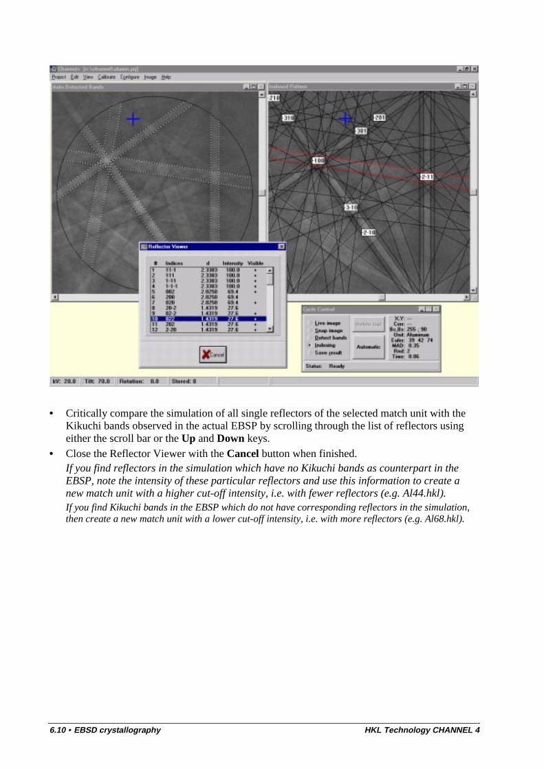
6.10 • EBSD crystallography HKL Technology CHANNEL 4
• Critically compare the simulation of all single reflectors of the selected match unit with theKikuchi bands observed in the actual EBSP by scrolling through the list of reflectors usingeither the scroll bar or the Up and Down keys.
• Close the Reflector Viewer with the Cancel button when finished.If you find reflectors in the simulation which have no Kikuchi bands as counterpart in theEBSP, note the intensity of these particular reflectors and use this information to create anew match unit with a higher cut-off intensity, i.e. with fewer reflectors (e.g. Al44.hkl).If you find Kikuchi bands in the EBSP which do not have corresponding reflectors in the simulation,then create a new match unit with a lower cut-off intensity, i.e. with more reflectors (e.g. Al68.hkl).
HKL Technology CHANNEL 4 EBSD crystallography • 6.11
An alternative way to find the Cut-off intensity
Another way to determine the cut-off intensity of a match unit usedin the indexing procedure within CHANNEL - Acquisition is thefollowing:
• Create a new match unit with a relatively low cut-off intensity, i.e. with many reflectors (e.g.Al84.hkl). Refer to the section called Creating a Match Unit.
• Automatically detect the Kikuchi bands and index the EBSP using this new match unit.
• Select Configure | Display of simulation… from the menu bar to reveal the Display ofMatch Unit dialog box.
• Experiment with different values to be entered in the Minimum intensity edit box. Click onOK to see the difference in the simulations for the varying minimum intensities. Note theminimum intensity for which the simulation fits the actual EBSP best and create a new matchunit with an appropriate cut-off intensity. Refer to the section called Critical choice ofreflectors used in the match unit.
Note: The Display of Match Unit dialog box you allows to choosebetween a display of the Center of bands or Edges of bands byselecting the appropriate radio button under Simulated lines along.To compare an EBSP and its simulation with regard to choosingthe number of reflectors, it might be more convenient to selectCenter of bands.

HKL Technology CHANNEL 4 EBSD - running an experiment • 7.1
EBSD - running an experiment
IntroductionTo run a experiment, i.e. to measure single crystallite orientationsby acquiring and indexing EBSPs from a crystalline material, it isnecessary that the EBSP system and the CHANNEL - Acquisitionsoftware package has been properly installed, that the system hasbeen calibrated and that the crystal structures encountered in thematerial have been defined.
Each experiment has to be assigned to a Project within CHANNEL- Acquisition. A project file(*.PRJ) contains all relevantinformation about the experiment and is internally linked to arecord file(*.REC) where the orientation data is stored. These filescan later be used for further processing of orientation ormisorientation data. This chapter describes the single procedures inCHANNEL - Acquisition of how to obtain orientation data derivedfrom EBSPs on a routine basis.
Acquiring an EBSPTo acquire an EBSP with your system several steps on the SEMand its EBSP hardware have to be carried out before using theCHANNEL - Acquisition software. Because of the considerabledifferences between SEMs and EBSP systems, only generalisedinstructions for their application can be given. If in doubt consultthe relevant manufacturers manuals. The following describes acommon procedure of how to produce an EBSP in the SEM. Referto the section called CHANNEL - Acquisition EBSD Acquisition.
• Switch on the SEM, EBSP computer and related equipment.
• Place the specimen and/or calibration sample in the SEM tilted to ~70° from the horizontaland facing the EBSP detector unit.
• Carefully align the reference direction of the specimen and/or calibration sample with respectto each other and the microscope axes by using the machined edges of the specimen stage.
7.2 • EBSD - running an experiment HKL Technology CHANNEL 4
• If your SEM has an eucentric stage to rotate the specimen and/or calibration sample about itssurface normal then align the reference direction within the microscopic image on the SEMscreen accurately (refer to the section called Calibration guidelines for details).
Note: Accurate alignment of the specimen and/or calibrationsample in the SEM is critical for obtaining a correct calibration andreliable orientation data. For an EBSP calibration to be valid it isnecessary to keep the specimen position with regard to the electronbeam fixed. This can be accomplished by not changing themicroscope’s focus control and always bring the specimen backinto focus by using the specimen stage Z-control.
• Pump down the microscope. Switch on the SEM filament and adjust to normal operatingconditions for which the existing calibration is valid: e.g. 20-30mm working distance, 20kVacceleration voltage, ~1-20nA beam current (depending on the sensitivity of the EBSPcamera).
• Produce a secondary electron image (in the SEM image mode) of a region of the specimen orcalibration sample, a magnification of 200 is adequate. Focus this image by using the Z-control.
• Switch the SEM into spot mode- this directs the beam to a single point on the specimenallowing an EBSP to be produced and to be viewed on the phosphor screen.
• Switch on the EBSP detector unit and any other related equipment, e.g. an image processor.
Note: Some EBSP cameras, e.g. SITs, can be damaged by roomlighting - be careful to switch them off when opening the SEMchamber door.
• Examine the generated EBSP image on a separate EBSP monitor (and/or in CHANNEL -Acquisition on the PC monitor - see below) - it should consist of many Kikuchi bands withdifferent width and brightness.
• Switch the SEM back into image mode and perform a background subtraction on the imageprocessor attached to the EBSP camera, using the fastest possible scan rate.
• Switch the SEM back into spot mode to see the success of the background subtraction andoptimise contrast and brightness of the EBSP image.
• Move the electron beam or specimen to acquire further EBSPs and make sure that they are ofgood quality.
Having produced some good quality EBSPs under the operatingconditions for which the existing calibration is valid, it is nowpossible to make orientation measurements using the CHANNEL -Acquisition software.

HKL Technology CHANNEL 4 EBSD - running an experiment • 7.3
Starting CHANNEL - Acquisition and configuring thesystem
Run CHANNEL - Acquisition• Start the main program Channel by double clicking on the CHANNEL - Acquisition icon.
• Select Project | New... in the start-up menu bar. Enter a name for the new project file (*.PRJ)under File Name, change directory if necessary. Click on OK.The main program screen, which comprises the Auto Detected Bands (left) and IndexedPattern (right) windows, plus the Cycle Control window will appear. The Auto DetectedBands window will show a live EBSP image as relayed by the EBSP detector unit.By selecting Snap image in the Cycle Control dialog box it will be frozen and also displayedin the Indexed Pattern window (see Fig 3.8).
Define Match Unit(s), AOI and SEM conditions• Load a match unit by selecting Project | Match units... in the menu bar. The Match Units
dialog box will appear on screen. Click on the Add button to reveal the Load Match Unitdialog box.
• Choose the required file from the list and click on OK, change directory if necessary.N.B. HKL files are usually in the COMMON directory.
• You can add more match units if you want. Click on when OK finished.The Indexing and Save result radio buttons and the Automatic button, located in the CycleControl dialog box, are now enabled.
• If the SEM conditions have changed, you will need to load a calibration by selectingCalibrate | Load…in the menu bar. Select a calibration file (*.CAL), N.B. change directoryif needed. Click on OK to accept the selection.
• Enter the area of interest (AOI) by selecting Configure | Area of interest (AOI) in the menubar. Click on the circle with the Left Mouse Button and drag the circle to a suitable place.You can scale the circle by clicking with the Right Mouse Button and moving the mouse.Close the window (top left icon) to accept the changes..
• Enter the SEM operating conditions (acceleration voltage, kV and stage tilt, °) by selectingConfigure | SEM conditions... in the menu bar. The SEM conditions dialog box will appearon the screen. Enter the values if different from the pre-set operating conditions. Click on OKto accept the changes.
For further configuration options under Configure in the menurefer to the chapters below.
7.4 • EBSD - running an experiment HKL Technology CHANNEL 4
Manually detecting bandsCHANNEL - Acquisition has facilities for automatically detectingKikuchibands, however when working with poorer quality EBSPsor when calibrating the system it is often better to manually markthe Kikuchi bands. This usually results in a more accuratemeasurement.
You have the choice of either marking the centre of the Kikuchibandor its edges. It is recommended that wherever possible, youmark the band edges as this is usually more accurate. However,when Kikuchi bands are narrow, it is acceptable to detect the bandcentres.
Switching to Manual Detection mode• Deselect the automatic detection of Kikuchi bands by selecting View | Auto detect bands.
The tick (ä) symbol will be removed and the title of the left window will change from AutoDetected Bands to Manually Detected Bands. The cursor, in the Manually Detected Bandswindow, will now appear as a white cross with a black dot at its centre.
How many Kikuchi Bands should I Use ?
For reliable indexing, manually detect between 4 and 8 Kikuchibands depending on the quality of the EBSP.
The following table gives guidance on the number of Kikuchibands to use based on the number of reflectors in the match unit.
Number of Reflectors 40 to 59 60 to 69 70 to 99 100 plusNumber of Kikuchi Bands 4 to 5 5 to 6 6 to 7 6 to 8
Which Kikuchi Bands should I Mark ?
Try to make sure that the Kikuchi bands you select are equallyspaced out across the EBSP, both around the pattern centre and theimage edges. This will result in a more accurate indexing.
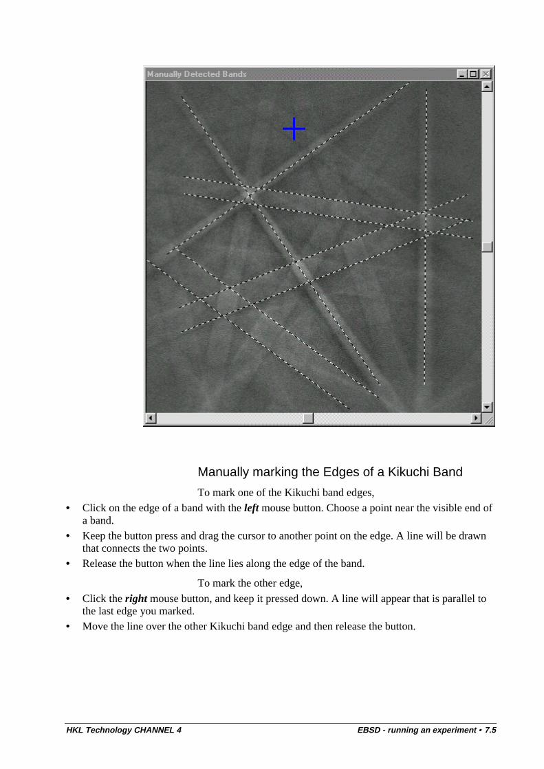
HKL Technology CHANNEL 4 EBSD - running an experiment • 7.5
Manually marking the Edges of a Kikuchi Band
To mark one of the Kikuchi band edges,
• Click on the edge of a band with the left mouse button. Choose a point near the visible end ofa band.
• Keep the button press and drag the cursor to another point on the edge. A line will be drawnthat connects the two points.
• Release the button when the line lies along the edge of the band.
To mark the other edge,
• Click the right mouse button, and keep it pressed down. A line will appear that is parallel tothe last edge you marked.
• Move the line over the other Kikuchi band edge and then release the button.
7.6 • EBSD - running an experiment HKL Technology CHANNEL 4
Manually marking the Centre of a Kikuchi Band
To mark the centre of the Kikuchi band,
• Click on the centre of a band with the left mouse button. Choose a point near the visible endof a band.
• Keep the button press and drag the cursor to another point along the centre of the band. A linewill be drawn that connects the two points.
• Release the button when the line lies along the edge of the band.
Deleting Bands
You may decide that you want to remove one or more of the bandsthat you have marked, this is done as follows.
• Select Edit | Browse bands or• Press Page Down key on the keyboard. The last band you marked will be highlighted in red.• Either : press the Delete key to remove it,• Or, press Page Down until the band you wish to remove is highlighted, then press Delete.
You can delete all the bands by pressing the Edit | Remove all bands menu item or bypressing the Shift and Delete keys together. You can also use the Edit | Cut band menu itemto delete a single band.
Automatically detecting bandsCHANNEL - Acquisition has the facility to rapidly and reliablydetect Kikuchi bands using automatic image processing andanalysis methods.
• Deselect the manual detection of Kikuchi bands by selecting View | Auto detect bands in themenu bar. The tick (ä) symbol will reappear and the header in the left window will changefrom Manually Detected Bands to Auto Detected Bands.
• Configure the parameters for the automatic band detection by selecting Configure | CycleControl...in the menu bar (refer to the section called the Cycle Control Window for details).The Configure Cycle Control dialog box will appear
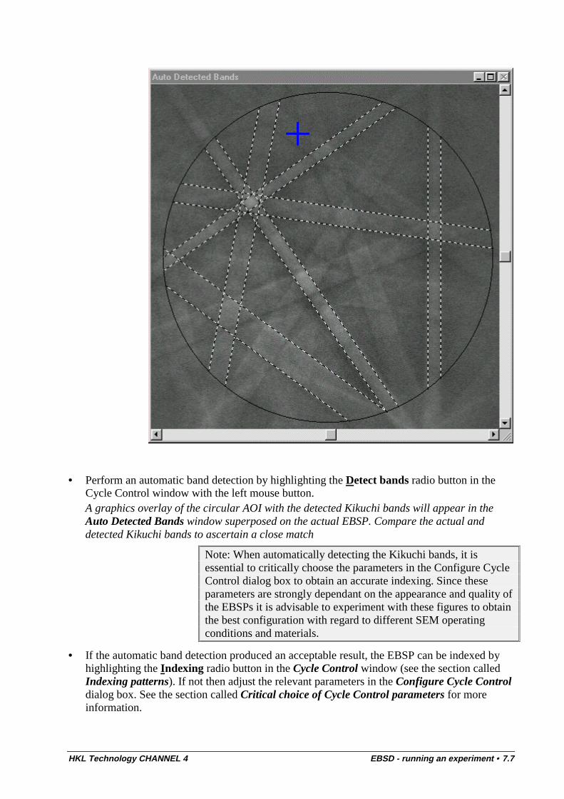
HKL Technology CHANNEL 4 EBSD - running an experiment • 7.7
• Perform an automatic band detection by highlighting the Detect bands radio button in theCycle Control window with the left mouse button.A graphics overlay of the circular AOI with the detected Kikuchi bands will appear in theAuto Detected Bands window superposed on the actual EBSP. Compare the actual anddetected Kikuchi bands to ascertain a close match
Note: When automatically detecting the Kikuchi bands, it isessential to critically choose the parameters in the Configure CycleControl dialog box to obtain an accurate indexing. Since theseparameters are strongly dependant on the appearance and quality ofthe EBSPs it is advisable to experiment with these figures to obtainthe best configuration with regard to different SEM operatingconditions and materials.
• If the automatic band detection produced an acceptable result, the EBSP can be indexed byhighlighting the Indexing radio button in the Cycle Control window (see the section calledIndexing patterns). If not then adjust the relevant parameters in the Configure Cycle Controldialog box. See the section called Critical choice of Cycle Control parameters for moreinformation.
7.8 • EBSD - running an experiment HKL Technology CHANNEL 4
Principles of automatic band detection
The automated detection of Kikuchi bands is based on a Houghtransformation which converts the EBSP band pattern into an arrayof maxima, where each of the maxima represents one diffractionband. The band detection is controlled by 3 interacting criteriawhich are applied in the following order:
• The intensity of Kikuchi bands should be high (i.e. higher diffracting lattice planes are morelikely to be detected, but see 2. and 3.)
• The Kikuchi bands should be spread throughout the EBSP (i.e. Kikuchi bands not only fromthe high-intensity projection centre, but also towards the margin of the area of interest(AOI)are detected)
• The intensity profile of the Kikuchi bands should be symmetrical (i.e. Kikuchi bands whichdo not have an equal intensity across their width and two distinct intensity minimacharacterising their margins are less likely to be detected - this applies for both: band centreor edge detection).
It is a strength of the Hough transformation in the CHANNEL -Acquisition software that there is no lower limit for the intensity ofKikuchi bands in the EBSP. Therefore it facilitates analyses evendown to on rather low quality EBSP images. However, the betterthe EBSP quality, the better the automatic band detection.
Note: For a good performance of the Hough transformation it isalso critical to set the limits of the AOI for a maximum area whichshow a good quality EBSP image. Be careful not to drag the AOIbeyond any of the straight image borders, since this may cause theHough transformation to detect a band there.
Critical choice of cycle control parametersThe performance of the automatic band detection is stronglydependent on the appearance and quality of the acquired EBSPs,which in turn are dependant on many parameters like SEMoperating conditions, material, surface quality, performance ofEBSP detector unit, etc. Therefore, to obtain the best configurationwith regard to accuracy and speed of band detection and indexing,it is advisable to spend some time experimenting with the figureswithin the Configure Cycle Control window by comparing theautomatically detected Kikuchi bands and the indexing/simulationscarefully.
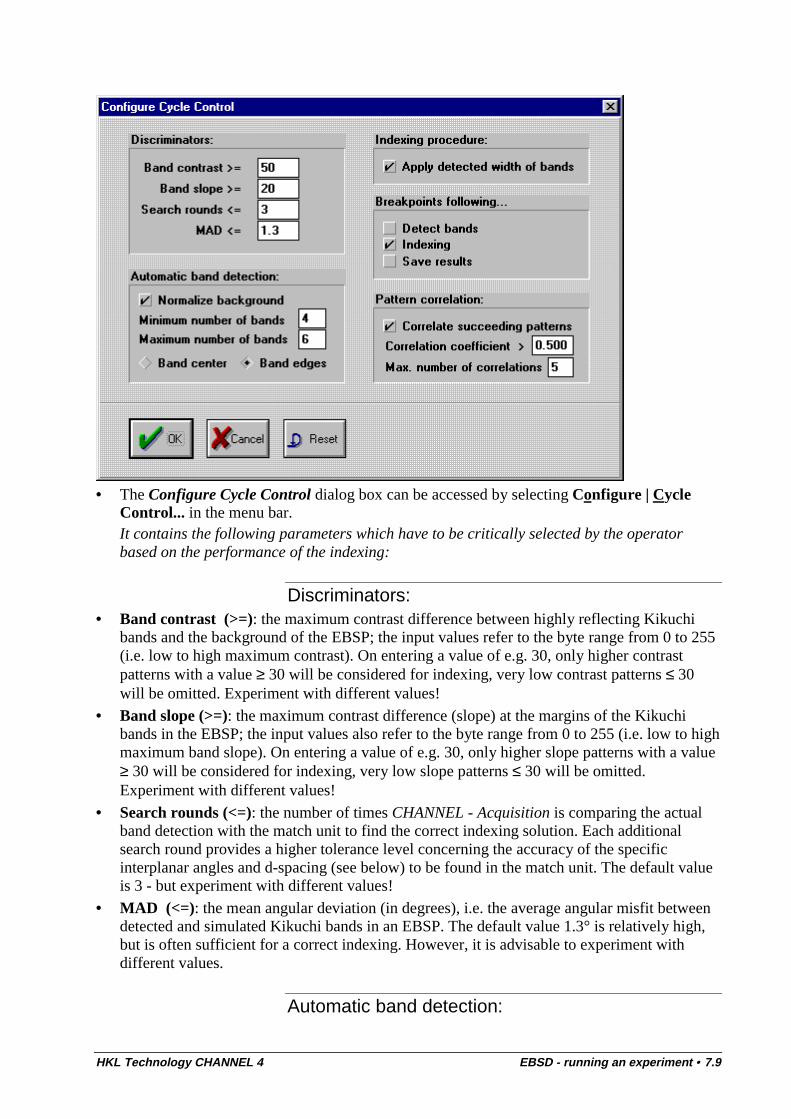
HKL Technology CHANNEL 4 EBSD - running an experiment • 7.9
• The Configure Cycle Control dialog box can be accessed by selecting Configure | CycleControl... in the menu bar.It contains the following parameters which have to be critically selected by the operatorbased on the performance of the indexing:
Discriminators:• Band contrast (>=): the maximum contrast difference between highly reflecting Kikuchi
bands and the background of the EBSP; the input values refer to the byte range from 0 to 255(i.e. low to high maximum contrast). On entering a value of e.g. 30, only higher contrastpatterns with a value ≥ 30 will be considered for indexing, very low contrast patterns ≤ 30will be omitted. Experiment with different values!
• Band slope (>=): the maximum contrast difference (slope) at the margins of the Kikuchibands in the EBSP; the input values also refer to the byte range from 0 to 255 (i.e. low to highmaximum band slope). On entering a value of e.g. 30, only higher slope patterns with a value≥ 30 will be considered for indexing, very low slope patterns ≤ 30 will be omitted.Experiment with different values!
• Search rounds (<=): the number of times CHANNEL - Acquisition is comparing the actualband detection with the match unit to find the correct indexing solution. Each additionalsearch round provides a higher tolerance level concerning the accuracy of the specificinterplanar angles and d-spacing (see below) to be found in the match unit. The default valueis 3 - but experiment with different values!
• MAD (<=): the mean angular deviation (in degrees), i.e. the average angular misfit betweendetected and simulated Kikuchi bands in an EBSP. The default value 1.3° is relatively high,but is often sufficient for a correct indexing. However, it is advisable to experiment withdifferent values.
Automatic band detection:
7.10 • EBSD - running an experiment HKL Technology CHANNEL 4
• Normalize background: a functionality by which the live EBSP image is processed toproduce a dynamic background for a more reliable performance of the Hough transformduring automatic band detection. On selecting this check box, unevenly illuminated EBSPimages are averaged out before the Hough transform is applied. Although you cannot see theeffect of this background normalisation directly in the image (this has been omitted due tokeep up the high performance speed), you can see its effect in the band detection -experiment! This functionality is probably of most use to users who cannot work on flatpolished sample surfaces.
• Minimum / Maximum number of bands: to enter a minimum and maximum number ofbands to be automatically detected. The numbers depend on how many bands are needed toobtain a correct indexing. Furthermore, considering the criteria for the automatic banddetection within CHANNEL - Acquisition it may be the case that in relatively low-qualityEBSPs a band may be detected wrongly. Hence, the program allows to input e.g. a minimumnumber of 5 and a maximum number of 6 to give a tolerance to leave out one band in theindexing.
• Detect band centres / band edges:: the facility to detect either the centre line or the edgelines of a Kikuchi band by selecting the appropriate radio buttons. The choice is alsodependant on the EBSP quality with regard to the criteria for the automatic band detectionwithin CHANNEL - Acquisition. Furthermore on selecting Detect band edges the d-spacinginformation can optionally applied to the indexing by also ticking the Apply detected width ofbands option described below.
Indexing procedure:• Apply detected width of bands: since the width of the Kikuchi bands is inversely
proportional to the lattice spacing (d), this option facilitates to use the lattice spacinginformation obtained by detecting the band edges (Detect band edges option) within theindexing procedure (refer to the section called Critical choice of Cycle Control parametersfor further details).
Breakpoints following…:
This functionality allows the user to set breaks within the automaticcycle for the cycle to stop at: Detect bands, Indexing or Saveresults.
It may be useful to check the performance of the band detection orthe indexing e.g. in problematic materials with a poor patternquality.
HKL Technology CHANNEL 4 EBSD - running an experiment • 7.11
Pattern correlation:
Note : Pattern correlation is not available in the US release of thesoftware.
This functionality is aimed at gaining further performance speedduring fully automatic EBSP measurements (utilising the add-onmodules: CHANNEL - Acquisition Beam and Stage Control). It ismeant to reduce the measurement time within grainareas ofidentical orientation in order to reduce the penalty of high over-sampling, e.g. when using small step sizes for the automatic gridmeasurements to gain a better microstructural reconstruction, orwhen investigating materials with a strong bimodal grain sizedistribution. It is based on correlating each pattern during the gridmeasurements with the previous one, and to check their differencebefore the band detection and indexing.
If the correlation coefficient (see below) is high, i.e. the differencebetween succeeding EBSPs is low, the pattern will be regarded asbeing identical with regard to the orientation of the previous one.Therefore the orientation data will be duplicated from the previousvalid indexing and the time involved for band detection andindexing is saved. The correlation always refers to the first validindexing made in an array of measurement points. As soon as thedeviation from this first indexing becomes more significant (i.e. thecorrelation coefficient due to lattice bending or grain boundaries),a new band detection and indexing takes place.
The correlation will not be performed on the basis of a zero-solution (no indexing solution) of an absent or very poor qualityEBSP signal, i.e. at grain boundaries, cracks, dislocation clusters,voids, inclusions or around damages on the sample surface. Thesoftware will try to index the following patterns until a validindexing solution is found. On every change in orientation, i.e.when crossing a grain boundary, there will always be a new banddetection and indexing.
• Correlate succeeding patterns: by selecting this check box, the fast correlation mode isactivated. It is recommended that the Normalize background function (see above) is turnedon for this operation.
• Correlation coefficient >: the correlation coefficient can be entered with values rangingfrom 0 (no correlation) to 1 (perfect correlation). For the analysis of EBSPs over apolycrystalline aggregate the frequency distribution of the correlation coefficient (x=0-1;y=%) normally describes a two-peak curve, with the first peak being related to non-correlatedpatterns of different grains or subgrains, a low being related to the superimposition of twopatterns of different grains or subgrains, and the second peak associated with highlycorrelated patterns within the same grain area bearing similar to equal orientations. Thissecond peak of the curve is the important one with regard to pattern correlation. Therefore thethreshold for the correlation coefficient should be set just at the bottom of the second peak,i.e. above the low between the two peaks (usually at about 0,3-0,5), at > 0,5, which is also the
7.12 • EBSD - running an experiment HKL Technology CHANNEL 4
default value. But it may be worth to experiment with this value, if you want to use thatfunctionality routinely. This can be done by doing several measurements within singledeformed grains with enough lattice bending to see sufficient deviations. The values for thecorrelation coefficient of each current measurement can be seen in the Cycle Control windowof CHANNEL - Acquisition under Corr:. During experimenting with the correlationcoefficient values, one always has to bare in mind, that the correlation is also stronglydependant on the image quality (i.e. the noise in the image) which in turn is dependant on theframe averaging of the external image processing, the probe current, the acceleration voltage,the surface quality and the materials characteristics.
• Max. number of correlations: this field requires an input of the maximum number ofcorrelations you will allow (default value: 5). The number is dependant on the over-samplingrate applied, i.e. how many consecutive measurement points will approximately have anidentical orientation within a single grain area, and therefore it depends on the average grainsize. However, as stated above, in the correlation mode, a new indexing will always takeplace when differences in the pattern correlation are detected (e.g. at grain boundaries). Thismax. number of correlations is therefore merely a restricting tool.
Indexing patternsTo perform an indexing of an acquired EBSP, the Kikuchi bandswould have to be detected previously, based on the manual orautomatic procedures described above, given that the calibration isvalid and that the appropriate match unit(s) has been loaded. Thefollowing steps describe the indexing procedure in CHANNEL -Acquisition after the previously outlined operational procedureshave been carried out.
• Click on the Indexing radio button in the Cycle Control dialog box with the left mousebutton to perform an automatic indexing and observe a simulated EBSP in the IndexedPattern window.
• Compare the actual and simulated EBSP to see whether they match.
• If the software has not produced a valid indexing, click on the Indexing radio button in theCycle Control window again and observe another simulation in the Indexed Pattern window.Repeat this procedure until pattern and simulation match. Refer also to the MAD number inthe Cycle Control window.
Note: Generally the software should produce a correct indexing onthe first attempt. However, if the software has not allowed a validindexing to take place after the third or more attempt, it is likelythat either the input of either match unit, the calibration or the SEMoperating conditions had been erroneous. In that case refer to thesection called EBSD system Calibration and Calibrationrefinements
Having achieved a valid indexing, i.e. a close match between theactual and simulated EBSP, it is now possible to see the result ofthe measurement in the Cycle Control. The displayed data isexplained in the Cycle control entry in the Glossary.
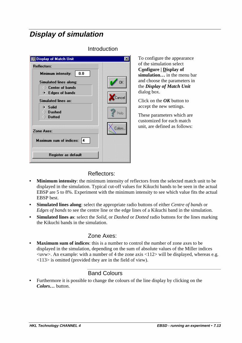
HKL Technology CHANNEL 4 EBSD - running an experiment • 7.13
Display of simulation
Introduction
To configure the appearanceof the simulation selectConfigure | Display ofsimulation… in the menu barand choose the parameters inthe Display of Match Unitdialog box.
Click on the OK button toaccept the new settings.
These parameters which arecustomized for each matchunit, are defined as follows:
Reflectors:• Minimum intensity : the minimum intensity of reflectors from the selected match unit to be
displayed in the simulation. Typical cut-off values for Kikuchi bands to be seen in the actualEBSP are 5 to 8%. Experiment with the minimum intensity to see which value fits the actualEBSP best.
• Simulated lines along: select the appropriate radio buttons of either Centre of bands orEdges of bands to see the centre line or the edge lines of a Kikuchi band in the simulation.
• Simulated lines as: select the Solid, or Dashed or Dotted radio buttons for the lines markingthe Kikuchi bands in the simulation.
Zone Axes:• Maximum sum of indices: this is a number to control the number of zone axes to be
displayed in the simulation, depending on the sum of absolute values of the Miller indices<uvw>. An example: with a number of 4 the zone axis <112> will be displayed, whereas e.g.<113> is omitted (provided they are in the field of view).
Band Colours• Furthermore it is possible to change the colours of the line display by clicking on the
Colors… button.
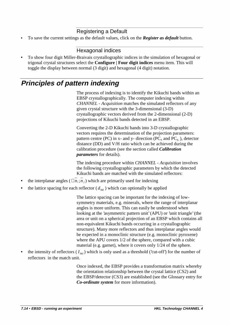
7.14 • EBSD - running an experiment HKL Technology CHANNEL 4
Registering a Default• To save the current settings as the default values, click on the Register as default button.
Hexagonal indices• To show four digit Miller-Braivais crystallographic indices in the simulation of hexagonal or
trigonal crystal structures select the Configure | Four digit indices menu item. This willtoggle the display between normal (3 digit) and hexagonal (4 digit) notation.
Principles of pattern indexingThe process of indexing is to identify the Kikuchi bands within anEBSP crystallographically. The computer indexing withinCHANNEL - Acquisition matches the simulated reflectors of anygiven crystal structure with the 3-dimensional (3-D)crystallographic vectors derived from the 2-dimensional (2-D)projections of Kikuchi bands detected in an EBSP.
Converting the 2-D Kikuchi bands into 3-D crystallographicvectors requires the determination of the projection parameters:pattern centre (PC) in x- and y- direction (PCx and PCy, ), detectordistance (DD) and V/H ratio which can be achieved during thecalibration procedure (see the section called Calibrationparameters for details).
The indexing procedure within CHANNEL - Acquisition involvesthe following crystallographic parameters by which the detectedKikuchi bands are matched with the simulated reflectors:
• the interplanar angles ( ∠n ni j; ) which are primarily used for indexing
• the lattice spacing for each reflector ( dhkl ) which can optionally be applied
The lattice spacing can be important for the indexing of low-symmetry materials, e.g. minerals, where the range of interplanarangles is more uniform. This can easily be understood whenlooking at the ’asymmetric pattern unit’ (APU) or ’unit triangle’ (thearea or unit on a spherical projection of an EBSP which contains allnon-equivalent Kikuchi bands occurring in a crystallographicstructure). Many more reflectors and thus interplanar angles wouldbe expected in a monoclinic structure (e.g. monoclinic pyroxene)where the APU covers 1/2 of the sphere, compared with a cubicmaterial (e.g. garnet), where it covers only 1/24 of the sphere.
• the intensity of reflectors ( Ihkl ) which is only used as a threshold (’cut-off’) for the number ofreflectors in the match unit.
Once indexed, the EBSP provides a transformation matrix wherebythe orientation relationship between the crystal lattice (CS2) andthe EBSP/detector (CS3) are established (see the Glossary entry forCo-ordinate system for more information).
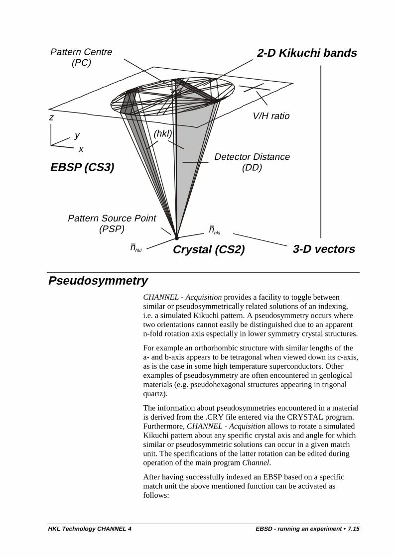
HKL Technology CHANNEL 4 EBSD - running an experiment • 7.15
V/H ratio
Pattern Centre(PC)
Detector Distance(DD)
Pattern Source Point(PSP)
2-D Kikuchi bands
3-D vectors
EBSP (CS3)
nhkl
nhkl
(hkl)
Crystal (CS2)
xy
z
PseudosymmetryCHANNEL - Acquisition provides a facility to toggle betweensimilar or pseudosymmetrically related solutions of an indexing,i.e. a simulated Kikuchi pattern. A pseudosymmetry occurs wheretwo orientations cannot easily be distinguished due to an apparentn-fold rotation axis especially in lower symmetry crystal structures.
For example an orthorhombic structure with similar lengths of thea- and b-axis appears to be tetragonal when viewed down its c-axis,as is the case in some high temperature superconductors. Otherexamples of pseudosymmetry are often encountered in geologicalmaterials (e.g. pseudohexagonal structures appearing in trigonalquartz).
The information about pseudosymmetries encountered in a materialis derived from the .CRY file entered via the CRYSTAL program.Furthermore, CHANNEL - Acquisition allows to rotate a simulatedKikuchi pattern about any specific crystal axis and angle for whichsimilar or pseudosymmetric solutions can occur in a given matchunit. The specifications of the latter rotation can be edited duringoperation of the main program Channel.
After having successfully indexed an EBSP based on a specificmatch unit the above mentioned function can be activated asfollows:
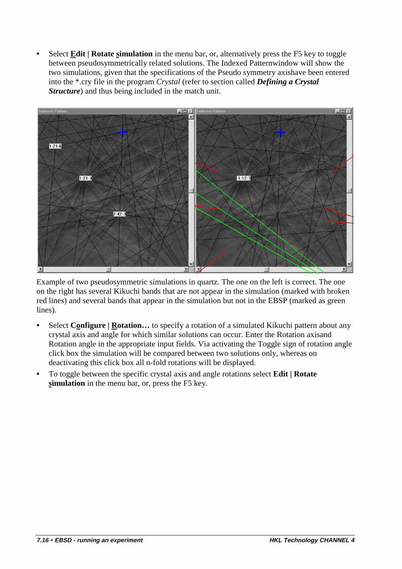
7.16 • EBSD - running an experiment HKL Technology CHANNEL 4
• Select Edit | Rotate simulation in the menu bar, or, alternatively press the F5 key to togglebetween pseudosymmetrically related solutions. The Indexed Patternwindow will show thetwo simulations, given that the specifications of the Pseudo symmetry axishave been enteredinto the *.cry file in the program Crystal (refer to section called Defining a CrystalStructure) and thus being included in the match unit.
Example of two pseudosymmetric simulations in quartz. The one on the left is correct. The oneon the right has several Kikuchi bands that are not appear in the simulation (marked with brokenred lines) and several bands that appear in the simulation but not in the EBSP (marked as greenlines).
• Select Configure | Rotation… to specify a rotation of a simulated Kikuchi pattern about anycrystal axis and angle for which similar solutions can occur. Enter the Rotation axisandRotation angle in the appropriate input fields. Via activating the Toggle sign of rotation angleclick box the simulation will be compared between two solutions only, whereas ondeactivating this click box all n-fold rotations will be displayed.
• To toggle between the specific crystal axis and angle rotations select Edit | Rotatesimulation in the menu bar, or, press the F5 key.
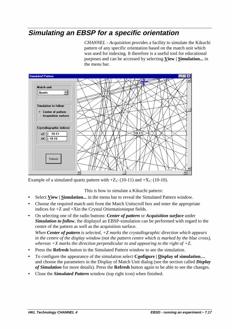
HKL Technology CHANNEL 4 EBSD - running an experiment • 7.17
Simulating an EBSP for a specific orientationCHANNEL - Acquisition provides a facility to simulate the Kikuchipattern of any specific orientation based on the match unit whichwas used for indexing. It therefore is a useful tool for educationalpurposes and can be accessed by selecting View | Simulation... inthe menu bar.
Example of a simulated quartz pattern with +Z1: (10-11) and +X1: (10-10).
This is how to simulate a Kikuchi pattern:• Select View | Simulation... in the menu bar to reveal the Simulated Pattern window.
• Choose the required match unit from the Match Unitscroll box and enter the appropriateindices for +Z and +Xin the Crystal Orientationinput fields.
• On selecting one of the radio buttons: Center of pattern or Acquisition surface underSimulation to follow, the displayof an EBSP-simulation can be performed with regard to thecentre of the pattern as well as the acquisition surface.When Center of pattern is selected, +Z marks the crystallographic direction which appearsin the centre of the display window (not the pattern centre which is marked by the blue cross),whereas +X marks the direction perpendicular to and appearing to the right of +Z.
• Press the Refresh button in the Simulated Pattern window to see the simulation.
• To configure the appearance of the simulation select Configure | Display of simulation…and choose the parameters in the Display of Match Unit dialog (see the section called Displayof Simulation for more details). Press the Refresh button again to be able to see the changes.
• Close the Simulated Pattern window (top right icon) when finished.
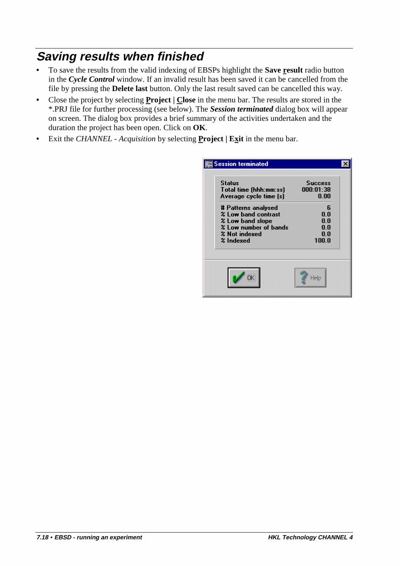
7.18 • EBSD - running an experiment HKL Technology CHANNEL 4
Saving results when finished• To save the results from the valid indexing of EBSPs highlight the Save result radio button
in the Cycle Control window. If an invalid result has been saved it can be cancelled from thefile by pressing the Delete last button. Only the last result saved can be cancelled this way.
• Close the project by selecting Project | Close in the menu bar. The results are stored in the*.PRJ file for further processing (see below). The Session terminated dialog box will appearon screen. The dialog box provides a brief summary of the activities undertaken and theduration the project has been open. Click on OK.
• Exit the CHANNEL - Acquisition by selecting Project | Exit in the menu bar.

HKL Technology CHANNEL 4 EBSD - running an experiment • 7.19
Automatic measurementsAll the main steps of the operational procedure, located in theCycle Control window, i.e. Live image, Snap image,Detect bands,Indexing and Save results can be carried out automatically byclicking on the Automatic button. This option has beenimplemented in the software to allow the user to perform numerousmeasurements within a short time. Furthermore it is required whenperforming fully automated measurements using the CHANNEL -Acquisition beam and stage control modules.
• On clicking the Automatic button steps in the EBSP cycle will then be carried out,highlighting the different radio buttons in the Cycle Control dialog box sequentially andfinally jumping back to Live image. For each successful automatic measurement the data willbe stored and displayed in the Cycle Control window (see the Glossary entry for “Cyclecontrol” for a description of the data).
• The number of stored results shown in the status bar will be incremented by one digit. If aninvalid result has been saved it can be cancelled from the file by pressing the Delete lastbutton.
Note: When performing automatic measurements, it is advisable tocarefully assess the performance of the band detection and indexingduring the first measurements of a project. It may be necessary tofurther fine-tune parameters of the experiment or to refine thecalibration.

HKL Technology CHANNEL 4 Mesotex - misorientations from operator measurements • 8.1
Mesotex - misorientations fromoperator measurements
IntroductionThe following sections describe the operational procedures tocalculate and display misorientation data from the orientationmeasurements carried out with CHANNEL - Acquisition.
Starting Mesotex• Start the misorientation program by double clicking on the Mesotex icon in the CHANNEL -
Acquisition software menu box - The CHANNEL - Acquisition MesoTexture program screenwill appear.
• Open a project by selecting: Project | Open... in the menu bar and select the appropriate*.PRJ file.
Creating misorientation data
Firstly, a list of combinations for pairs (usually neighbouring)crystallites has to be created, for which the misorientation is to becalculated in terms of axis/angle pairs.
• To produce such a list, select Combinations | Add.... The Generate Combinations dialogbox appears, showing a record browser for each crystallite (A and B) to be compared for thecalculation of the misorientation in terms of axis/angle pairs. Within this dialog box you caneither manually Add single combinations to the list or Combine successors, i.e. combineeach consecutive measurement.
• To add single combinations to the list, enter the consecutive numbers of the crystallites to becompared in the A=and B=input boxes, or simply highlight the appropriate data in the tworecord browsers. Press the Add button to write the combination to the list.
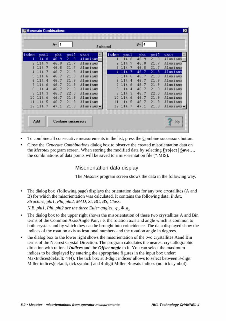
8.2 • Mesotex - misorientations from operator measurements HKL Technology CHANNEL 4
• To combine all consecutive measurements in the list, press the Combine successors button.
• Close the Generate Combinations dialog box to observe the created misorientation data onthe Mesotex program screen. When storing the modified data by selecting Project | Save…,the combinations of data points will be saved to a misorientation file (*.MIS).
Misorientation data display
The Mesotex program screen shows the data in the following way.
• The dialog box (following page) displays the orientation data for any two crystallites (A andB) for which the misorientation was calculated. It contains the following data: Index,Structure, phi1, Phi, phi2, MAD, St, BC, BS, Class.
N.B. phi1, Phi, phi2 are the three Euler angles, 21 ,, φφ Φ• The dialog box to the upper right shows the misorientation of these two crystallites A and Bin
terms of the Common Axis/Angle Pair, i.e. the rotation axis and angle which is common toboth crystals and by which they can be brought into coincidence. The data displayed show theindices of the rotation axis as irrational numbers and the rotation angle in degrees.
• the dialog box to the lower right shows the misorientation of the two crystallites Aand Binterms of the Nearest Crystal Direction. The program calculates the nearest crystallographicdirection with rational Indices and the Offset angle to it. You can select the maximumindices to be displayed by entering the appropriate figures in the input box under:MaxIndices(default: 444). The tick box at 3-digit indices’ allows to select between 3-digitMiller indices(default, tick symbol) and 4-digit Miller-Bravais indices (no tick symbol).
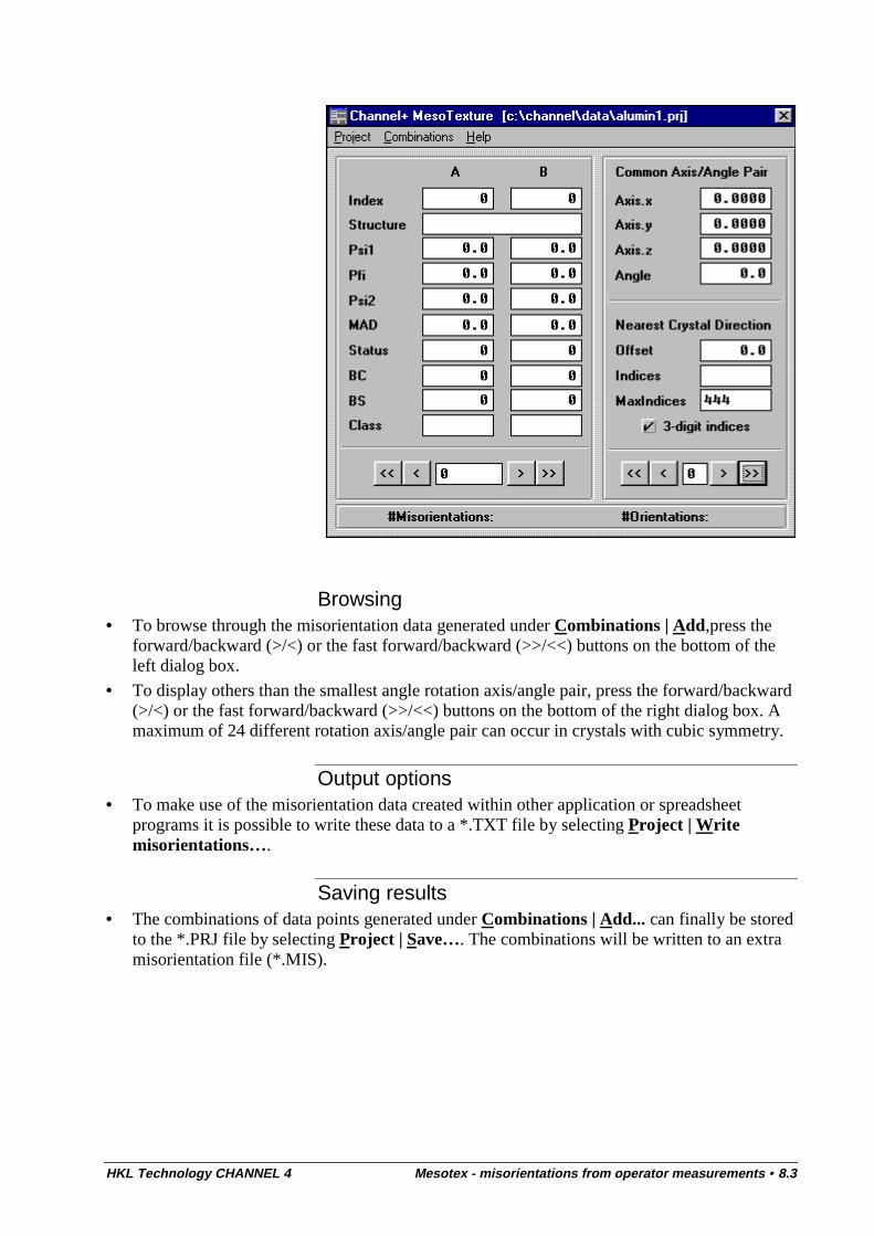
HKL Technology CHANNEL 4 Mesotex - misorientations from operator measurements • 8.3
Browsing• To browse through the misorientation data generated under Combinations | Add,press the
forward/backward (>/<) or the fast forward/backward (>>/<<) buttons on the bottom of theleft dialog box.
• To display others than the smallest angle rotation axis/angle pair, press the forward/backward(>/<) or the fast forward/backward (>>/<<) buttons on the bottom of the right dialog box. Amaximum of 24 different rotation axis/angle pair can occur in crystals with cubic symmetry.
Output options• To make use of the misorientation data created within other application or spreadsheet
programs it is possible to write these data to a *.TXT file by selecting Project | Writemisorientations….
Saving results• The combinations of data points generated under Combinations | Add... can finally be stored
to the *.PRJ file by selecting Project | Save…. The combinations will be written to an extramisorientation file (*.MIS).

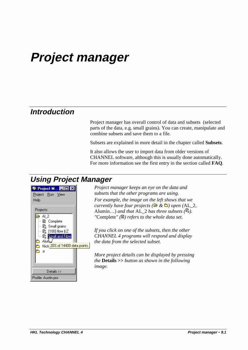
HKL Technology CHANNEL 4 Project manager • 9.1
Project manager
IntroductionProject manager has overall control of data and subsets (selectedparts of the data, e.g. small grains). You can create, manipulate andcombine subsets and save them to a file.
Subsets are explained in more detail in the chapter called Subsets.
It also allows the user to import data from older versions ofCHANNEL software, although this is usually done automatically.For more information see the first entry in the section called FAQ.
Using Project ManagerProject manager keeps an eye on the data andsubsets that the other programs are using.For example, the image on the left shows that wecurrently have four projects ( & ) open (AL_2,Alumin…) and that AL_2 has three subsets ( )."Complete" ( ) refers to the whole data set.
If you click on one of the subsets, then the otherCHANNEL 4 programs will respond and displaythe data from the selected subset.
More project details can be displayed by pressingthe Details >> button as shown in the followingimage.
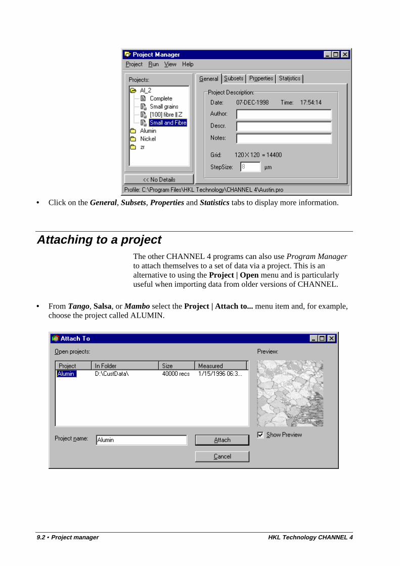
9.2 • Project manager HKL Technology CHANNEL 4
• Click on the General, Subsets, Properties and Statistics tabs to display more information.
Attaching to a projectThe other CHANNEL 4 programs can also use Program Managerto attach themselves to a set of data via a project. This is analternative to using the Project | Open menu and is particularlyuseful when importing data from older versions of CHANNEL.
• From Tango, Salsa, or Mambo select the Project | Attach to... menu item and, for example,choose the project called ALUMIN.
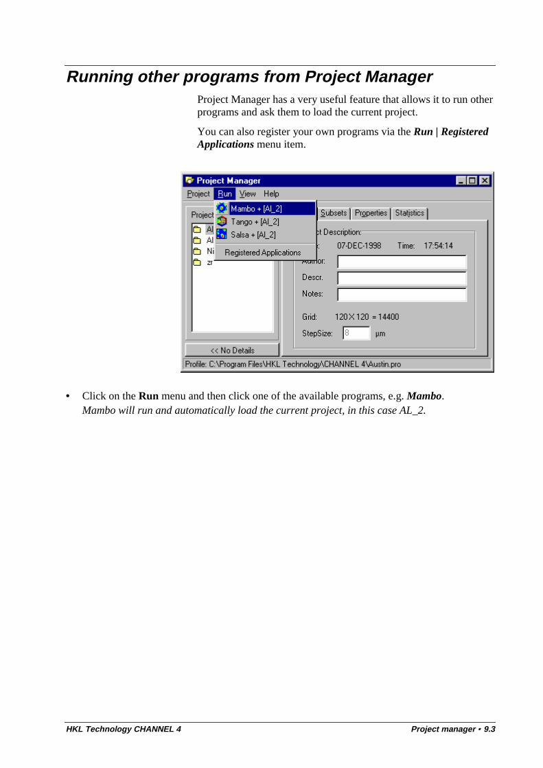
HKL Technology CHANNEL 4 Project manager • 9.3
Running other programs from Project ManagerProject Manager has a very useful feature that allows it to run otherprograms and ask them to load the current project.
You can also register your own programs via the Run | RegisteredApplications menu item.
• Click on the Run menu and then click one of the available programs, e.g. Mambo.Mambo will run and automatically load the current project, in this case AL_2.

HKL Technology CHANNEL 4 Mambo - (inverse) pole figures • 10.1
Mambo - (inverse) pole figures
IntroductionMambo is a tool for generating and Electron BackscatterDiffraction (EBSD) orientation data as pole figures and inversepole figures. The EBSD data can be obtained from either manual orfully automated EBSD measurements using CHANNEL+ or fromuser generated data via an ASCIItext file.
Mambo provides a flexible approach to the display andinterrogation of orientation and collected within a crystallinesample. It also allows the data to be interactively correlated withother microstructural information, e.g. in the new Tango orientationmapping software.
The following section is a step-by-step guide to running Mamboand importing an existing project. In this worked example theproject file is called AL_2.CPR and the orientation data is stored inAL_2.CRC.
Running Mambo
• Run the Mambo software by double-clicking on its icon, .Mambo is in the CHANNEL4 group under Programs, accessed by pressing the Windows™
Start button,
The following User Profile dialog box should appear :
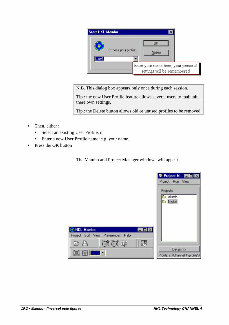
10.2 • Mambo - (inverse) pole figures HKL Technology CHANNEL 4
N.B. This dialog box appears only once during each session.
Tip : the new User Profile feature allows several users to maintainthere own settings.
Tip : the Delete button allows old or unused profiles to be removed.
• Then, either :• Select an existing User Profile, or• Enter a new User Profile name, e.g. your name.
• Press the OK button
The Mambo and Project Manager windows will appear :
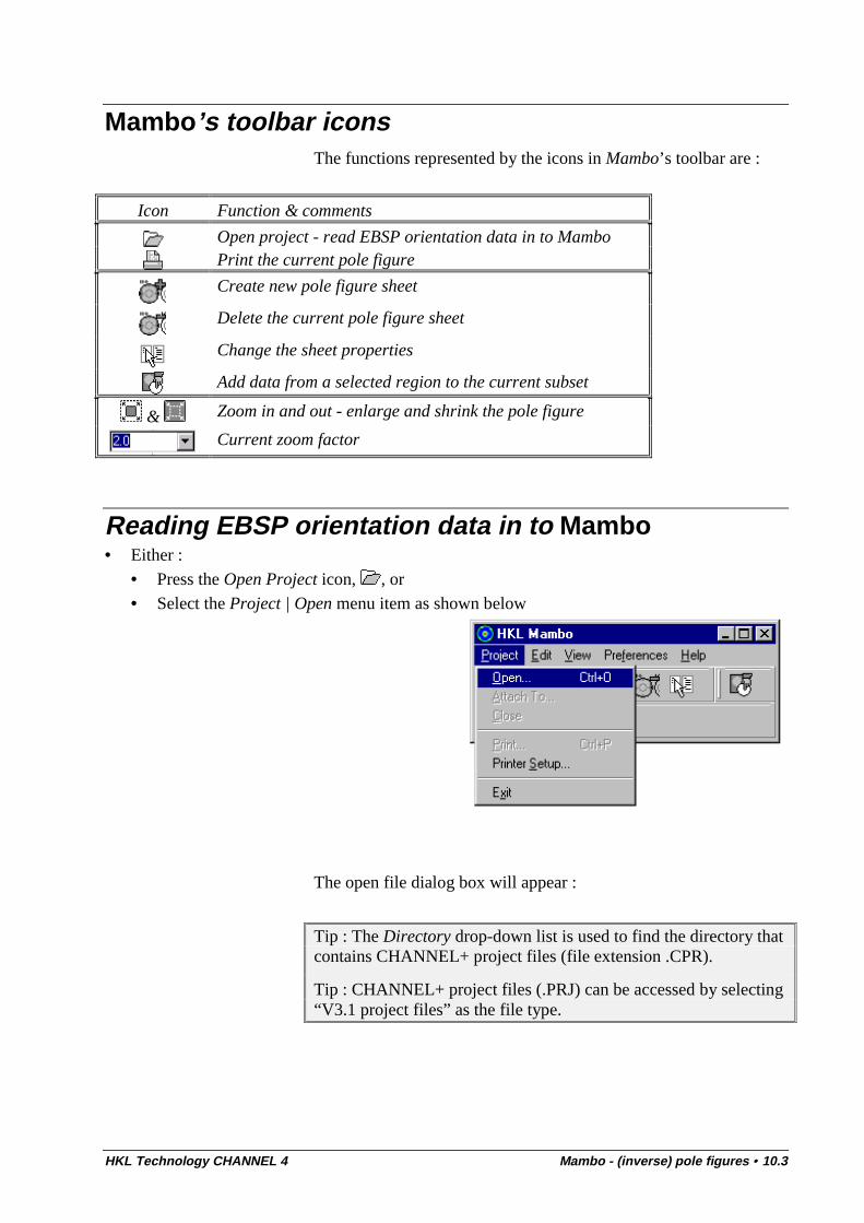
HKL Technology CHANNEL 4 Mambo - (inverse) pole figures • 10.3
Mambo’s toolbar iconsThe functions represented by the icons in Mambo’s toolbar are :
Icon Function & comments
Open project - read EBSP orientation data in to MamboPrint the current pole figure
Create new pole figure sheet
Delete the current pole figure sheet
Change the sheet properties
Add data from a selected region to the current subset
& Zoom in and out - enlarge and shrink the pole figure
Current zoom factor
Reading EBSP orientation data in to Mambo• Either :
• Press the Open Project icon, , or• Select the Project | Open menu item as shown below
The open file dialog box will appear :
Tip : The Directory drop-down list is used to find the directory thatcontains CHANNEL+ project files (file extension .CPR).
Tip : CHANNEL+ project files (.PRJ) can be accessed by selecting“V3.1 project files” as the file type.
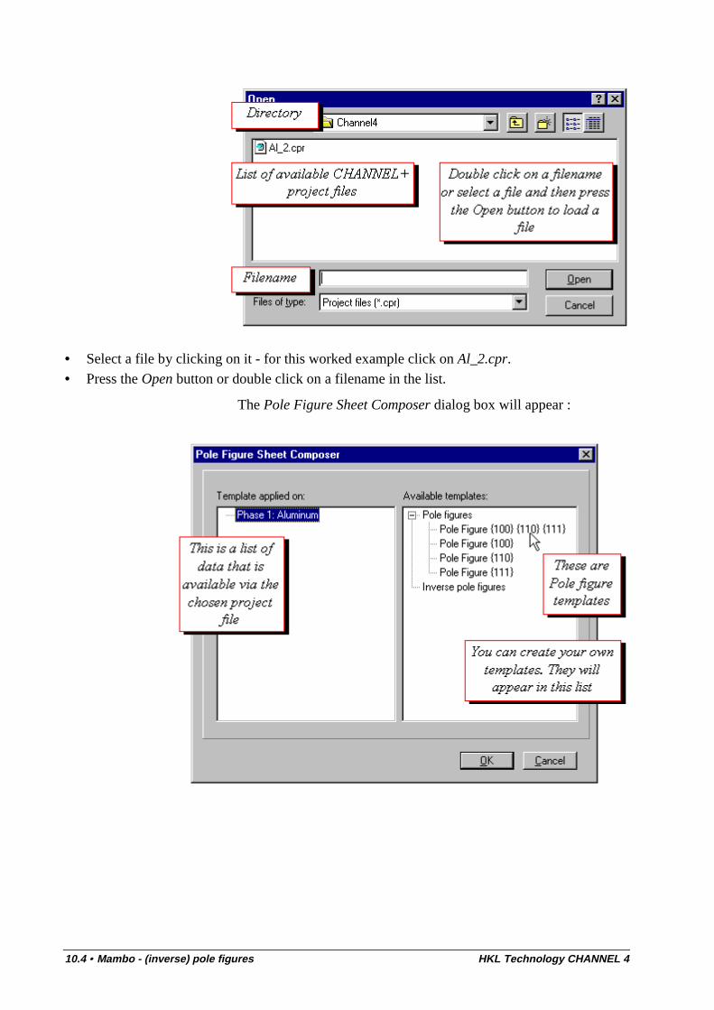
10.4 • Mambo - (inverse) pole figures HKL Technology CHANNEL 4
• Select a file by clicking on it - for this worked example click on Al_2.cpr.• Press the Open button or double click on a filename in the list.
The Pole Figure Sheet Composer dialog box will appear :
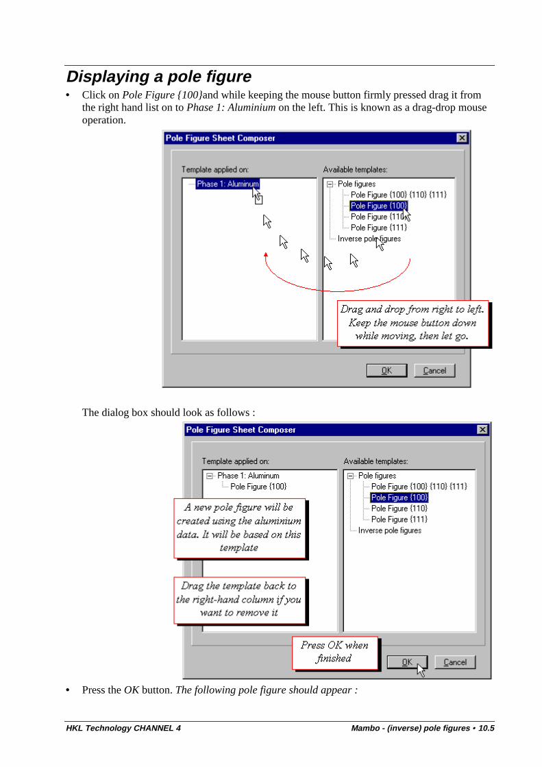
HKL Technology CHANNEL 4 Mambo - (inverse) pole figures • 10.5
Displaying a pole figure• Click on Pole Figure {100}and while keeping the mouse button firmly pressed drag it from
the right hand list on to Phase 1: Aluminium on the left. This is known as a drag-drop mouseoperation.
The dialog box should look as follows :
• Press the OK button. The following pole figure should appear :
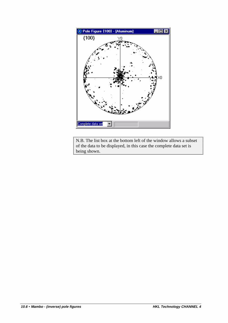
10.6 • Mambo - (inverse) pole figures HKL Technology CHANNEL 4
N.B. The list box at the bottom left of the window allows a subsetof the data to be displayed, in this case the complete data set isbeing shown.
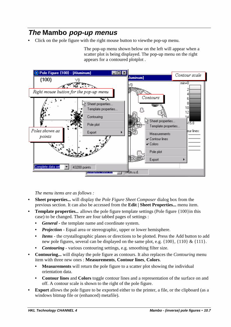
HKL Technology CHANNEL 4 Mambo - (inverse) pole figures • 10.7
The Mambo pop-up menus• Click on the pole figure with the right mouse button to viewthe pop-up menu.
The pop-up menu shown below on the left will appear when ascatter plot is being displayed. The pop-up menu on the rightappears for a contoured plotplot .
The menu items are as follows :
• Sheet properties... will display the Pole Figure Sheet Composer dialog box from theprevious section. It can also be accessed from the Edit | Sheet Properties... menu item.
• Template properties... allows the pole figure template settings (Pole figure {100}in thiscase) to be changed. There are four tabbed pages of settings :• General - the template name and coordinate system.• Projection - Equal area or stereographic, upper or lower hemisphere.
• Items - the crystallographic planes or directions to be plotted. Press the Add button to addnew pole figures, several can be displayed on the same plot, e.g. {100}, {110} & {111}.
• Contouring - various contouring settings, e.g. smoothing filter size.
• Contouring... will display the pole figure as contours. It also replaces the Contouring menuitem with three new ones : Measurements, Contour lines, Colors.
• Measurements will return the pole figure to a scatter plot showing the individualorientation data.
• Contour lines and Colors toggle contour lines and a representation of the surface on andoff. A contour scale is shown to the right of the pole figure.
• Export allows the pole figure to be exported either to the printer, a file, or the clipboard (as awindows bitmap file or (enhanced) metafile).
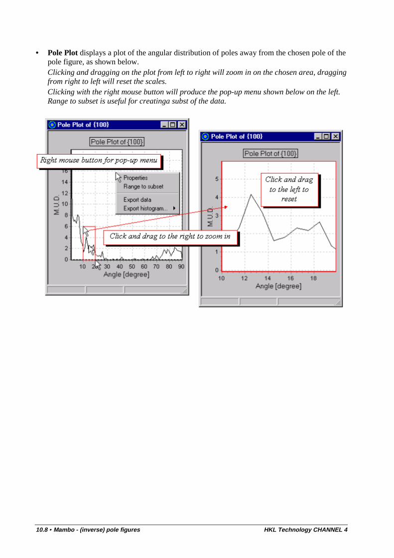
10.8 • Mambo - (inverse) pole figures HKL Technology CHANNEL 4
• Pole Plot displays a plot of the angular distribution of poles away from the chosen pole of thepole figure, as shown below.Clicking and dragging on the plot from left to right will zoom in on the chosen area, draggingfrom right to left will reset the scales.Clicking with the right mouse button will produce the pop-up menu shown below on the left.Range to subset is useful for creatinga subst of the data.
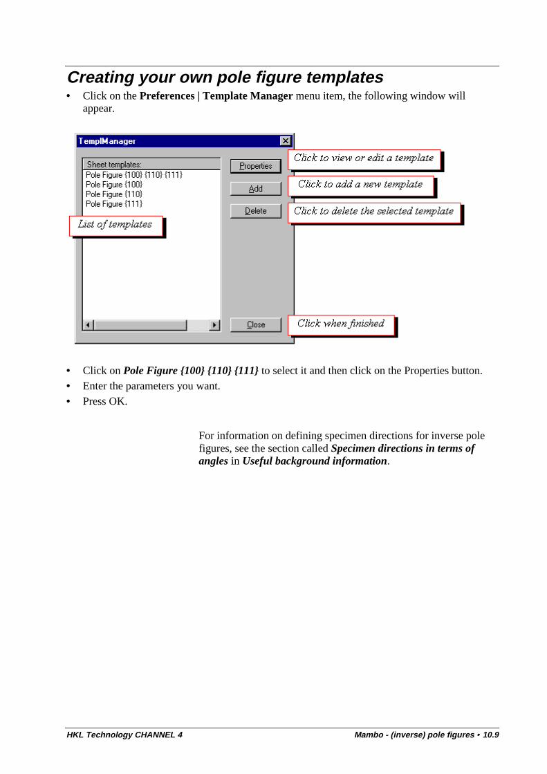
HKL Technology CHANNEL 4 Mambo - (inverse) pole figures • 10.9
Creating your own pole figure templates• Click on the Preferences | Template Manager menu item, the following window will
appear.
• Click on Pole Figure {100} {110} {111} to select it and then click on the Properties button.• Enter the parameters you want.• Press OK.
For information on defining specimen directions for inverse polefigures, see the section called Specimen directions in terms ofangles in Useful background information.

HKL Technology CHANNEL 4 Tango - mapping • 11.1
Tango - mapping
IntroductionTango is a software tool for generating, displaying and measuring awide variety of maps from Electron Backscatter Diffraction(EBSD) data, e.g. orientation, grain boundary, phase, patternquality. The EBSD data can be obtained from either manual orfully automated EBSP measurements using CHANNEL -Acquisition or from user generated data via an ASCII text file.
Tango also allows the data to be interactively correlated with otherinformation, e.g. in conjunction with the new Salsa (ODF)software.

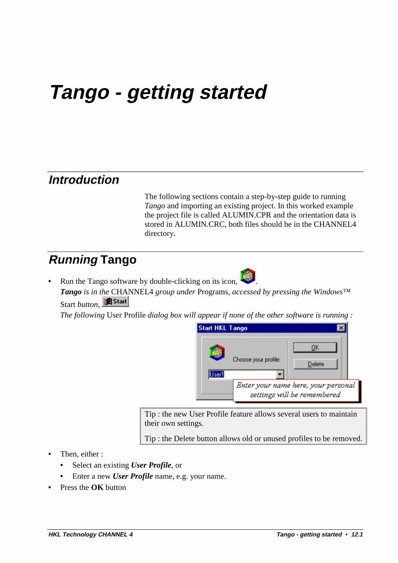
HKL Technology CHANNEL 4 Tango - getting started • 12.1
Tango - getting started
IntroductionThe following sections contain a step-by-step guide to runningTango and importing an existing project. In this worked examplethe project file is called ALUMIN.CPR and the orientation data isstored in ALUMIN.CRC, both files should be in the CHANNEL4directory.
Running Tango
• Run the Tango software by double-clicking on its icon, .Tango is in the CHANNEL4 group under Programs, accessed by pressing the Windows™
Start button, The following User Profile dialog box will appear if none of the other software is running :
Tip : the new User Profile feature allows several users to maintaintheir own settings.
Tip : the Delete button allows old or unused profiles to be removed.
• Then, either :• Select an existing User Profile, or• Enter a new User Profile name, e.g. your name.
• Press the OK button
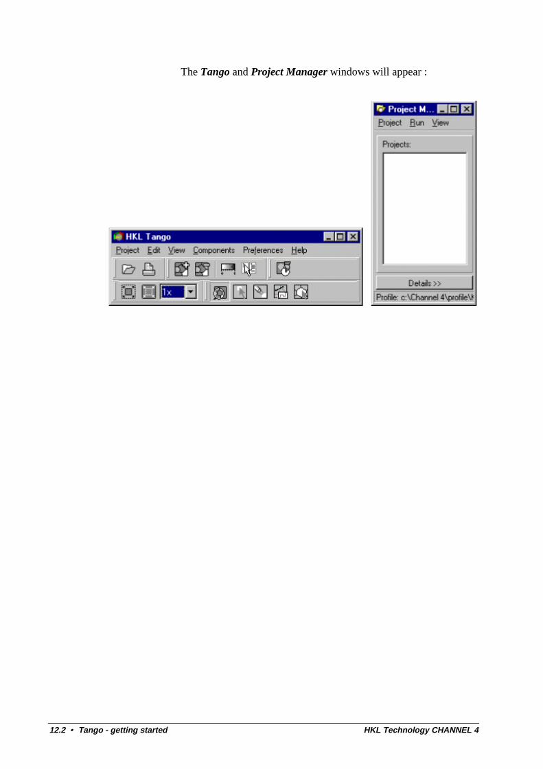
12.2 • Tango - getting started HKL Technology CHANNEL 4
The Tango and Project Manager windows will appear :
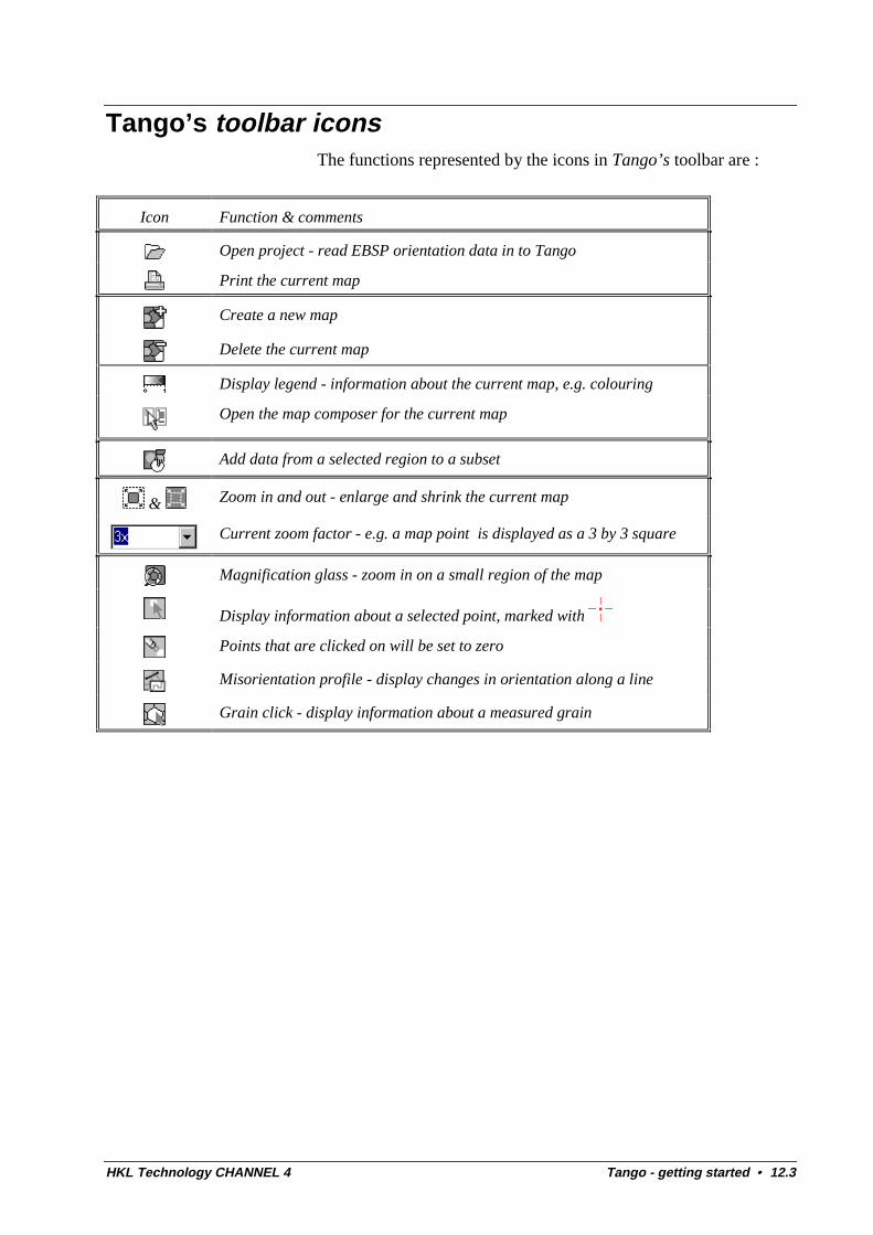
HKL Technology CHANNEL 4 Tango - getting started • 12.3
Tango’s toolbar iconsThe functions represented by the icons in Tango’s toolbar are :
Icon Function & comments
Open project - read EBSP orientation data in to Tango
Print the current map
Create a new map
Delete the current map
Display legend - information about the current map, e.g. colouring
Open the map composer for the current map
Add data from a selected region to a subset
& Zoom in and out - enlarge and shrink the current map
Current zoom factor - e.g. a map point is displayed as a 3 by 3 square
Magnification glass - zoom in on a small region of the map
Display information about a selected point, marked with
Points that are clicked on will be set to zero
Misorientation profile - display changes in orientation along a line
Grain click - display information about a measured grain
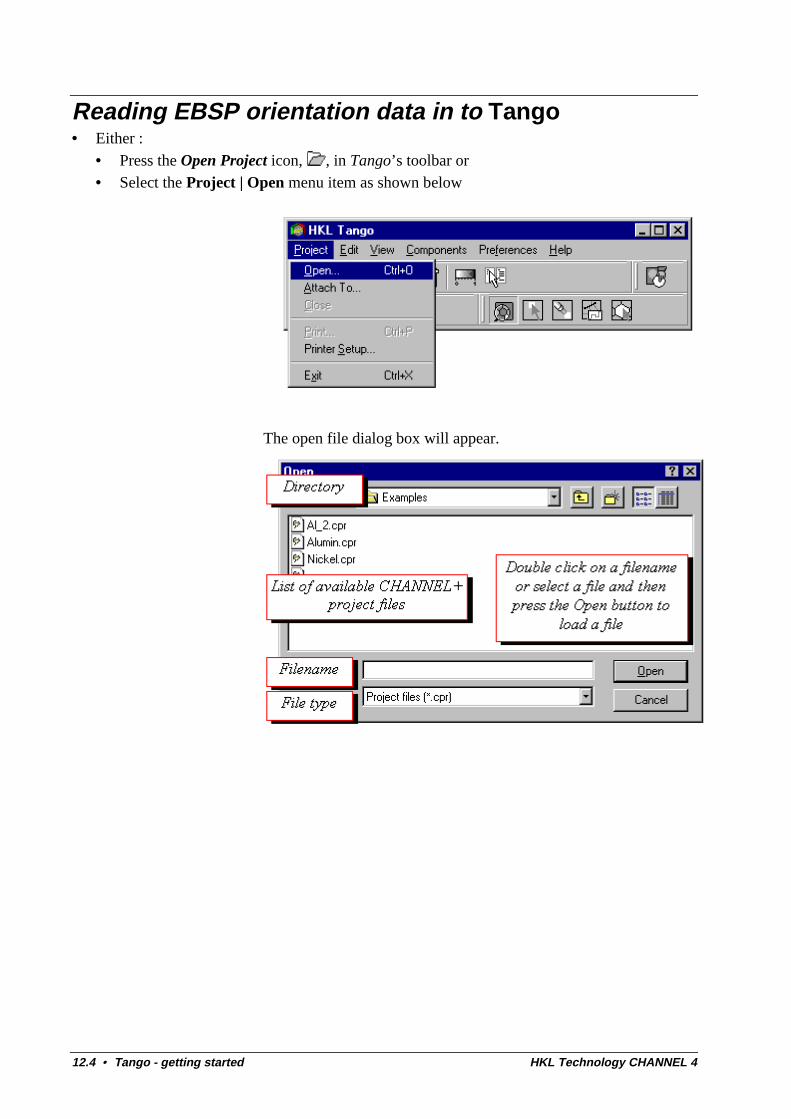
12.4 • Tango - getting started HKL Technology CHANNEL 4
Reading EBSP orientation data in to Tango• Either :
• Press the Open Project icon, , in Tango’s toolbar or• Select the Project | Open menu item as shown below
The open file dialog box will appear.
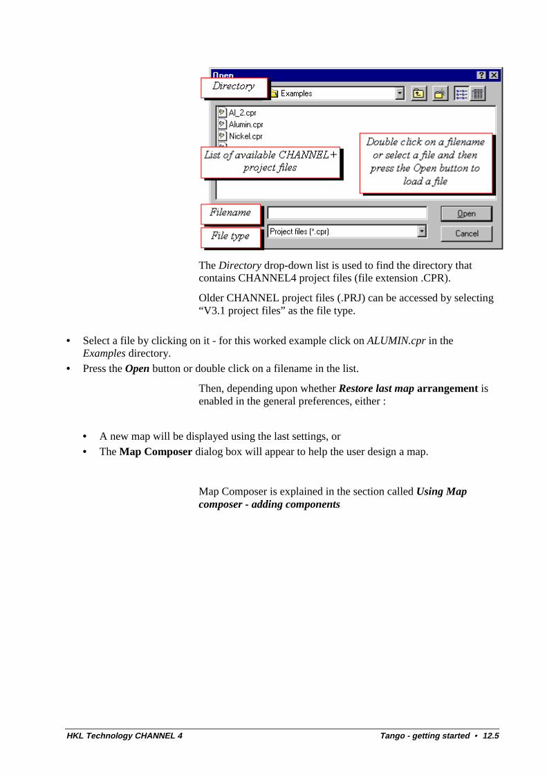
HKL Technology CHANNEL 4 Tango - getting started • 12.5
The Directory drop-down list is used to find the directory thatcontains CHANNEL4 project files (file extension .CPR).
Older CHANNEL project files (.PRJ) can be accessed by selecting“V3.1 project files” as the file type.
• Select a file by clicking on it - for this worked example click on ALUMIN.cpr in theExamples directory.
• Press the Open button or double click on a filename in the list.
Then, depending upon whether Restore last map arrangement isenabled in the general preferences, either :
• A new map will be displayed using the last settings, or• The Map Composer dialog box will appear to help the user design a map.
Map Composer is explained in the section called Using Mapcomposer - adding components
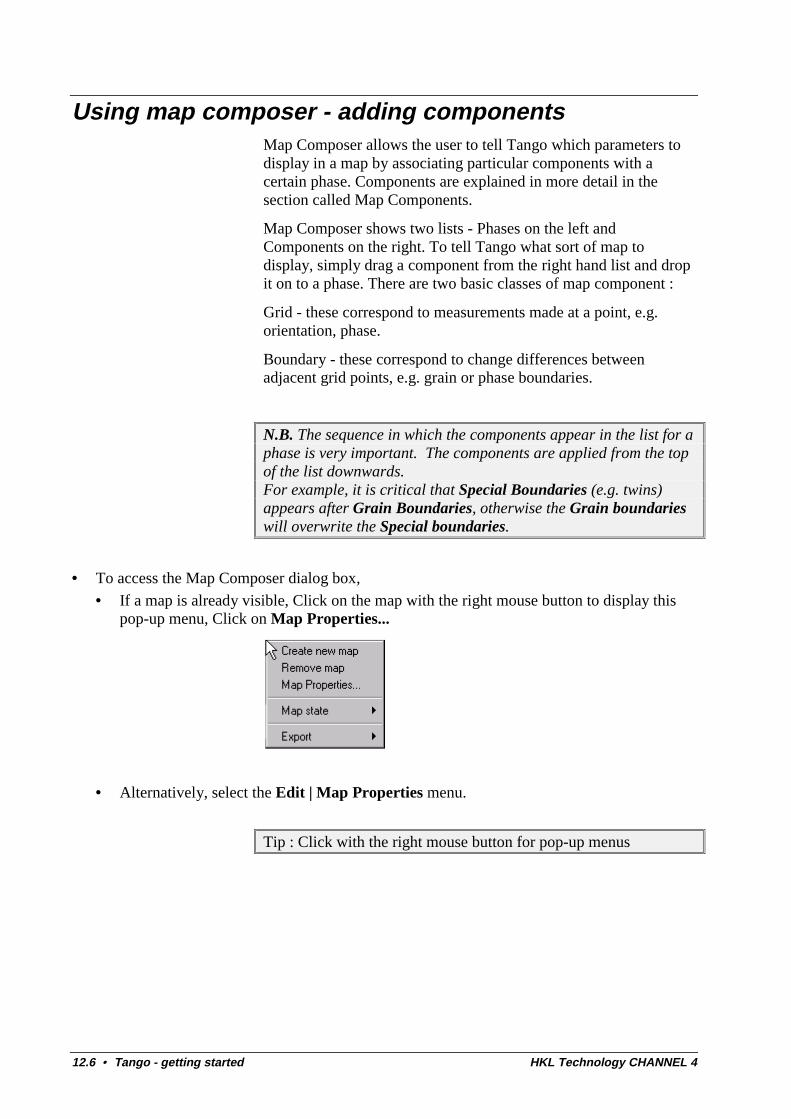
12.6 • Tango - getting started HKL Technology CHANNEL 4
Using map composer - adding componentsMap Composer allows the user to tell Tango which parameters todisplay in a map by associating particular components with acertain phase. Components are explained in more detail in thesection called Map Components.
Map Composer shows two lists - Phases on the left andComponents on the right. To tell Tango what sort of map todisplay, simply drag a component from the right hand list and dropit on to a phase. There are two basic classes of map component :
Grid - these correspond to measurements made at a point, e.g.orientation, phase.
Boundary - these correspond to change differences betweenadjacent grid points, e.g. grain or phase boundaries.
N.B. The sequence in which the components appear in the list for aphase is very important. The components are applied from the topof the list downwards.For example, it is critical that Special Boundaries (e.g. twins)appears after Grain Boundaries, otherwise the Grain boundarieswill overwrite the Special boundaries.
• To access the Map Composer dialog box,
• If a map is already visible, Click on the map with the right mouse button to display thispop-up menu, Click on Map Properties...
• Alternatively, select the Edit | Map Properties menu.
Tip : Click with the right mouse button for pop-up menus
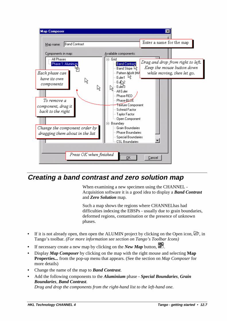
HKL Technology CHANNEL 4 Tango - getting started • 12.7
Creating a band contrast and zero solution mapWhen examining a new specimen using the CHANNEL -Acquisition software it is a good idea to display a Band Contrastand Zero Solution map.
Such a map shows the regions where CHANNELhas haddifficulties indexing the EBSPs - usually due to grain boundaries,deformed regions, contamination or the presence of unknownphases.
• If it is not already open, then open the ALUMIN project by clicking on the Open icon, , inTango’s toolbar. (For more information see section on Tango’s Toolbar Icons)
• If necessary create a new map by clicking on the New Map button, .
• Display Map Composer by clicking on the map with the right mouse and selecting MapProperties... from the pop-up menu that appears. (See the section on Map Composer formore details)
• Change the name of the map to Band Contrast.• Add the following components to the Aluminium phase - Special Boundaries, Grain
Boundaries, Band Contrast.Drag and drop the components from the right-hand list to the left-hand one.
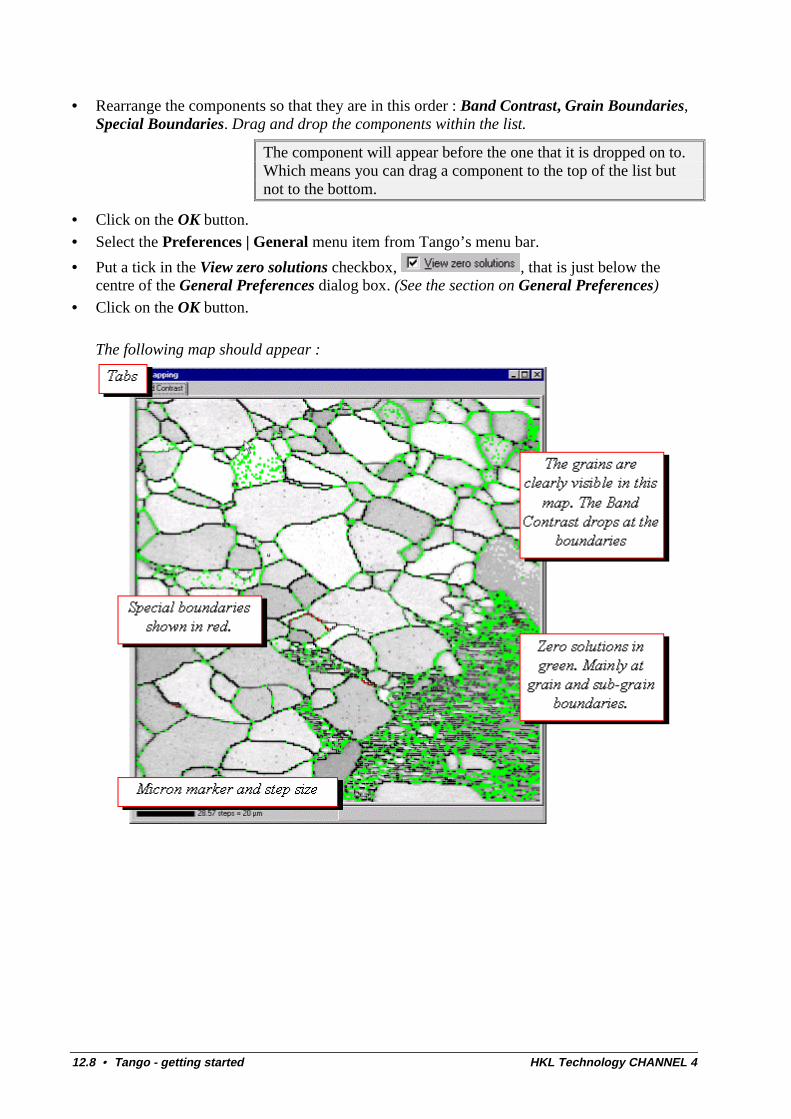
12.8 • Tango - getting started HKL Technology CHANNEL 4
• Rearrange the components so that they are in this order : Band Contrast, Grain Boundaries,Special Boundaries. Drag and drop the components within the list.
The component will appear before the one that it is dropped on to.Which means you can drag a component to the top of the list butnot to the bottom.
• Click on the OK button.• Select the Preferences | General menu item from Tango’s menu bar.
• Put a tick in the View zero solutions checkbox, , that is just below thecentre of the General Preferences dialog box. (See the section on General Preferences)
• Click on the OK button.
The following map should appear :
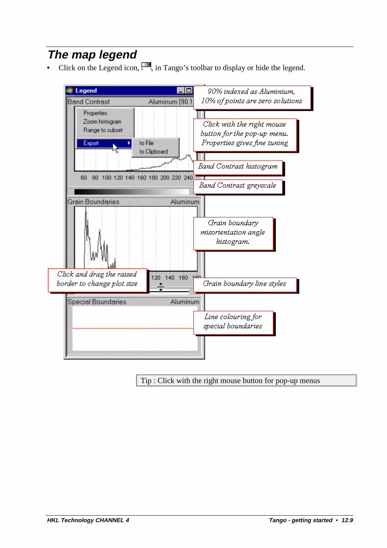
HKL Technology CHANNEL 4 Tango - getting started • 12.9
The map legend• Click on the Legend icon, , in Tango’s toolbar to display or hide the legend.
Tip : Click with the right mouse button for pop-up menus
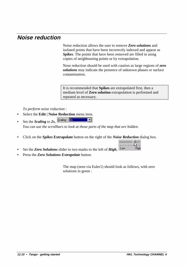
12.10 • Tango - getting started HKL Technology CHANNEL 4
Noise reductionNoise reduction allows the user to remove Zero solutions andisolated points that have been incorrectly indexed and appear asSpikes. The points that have been removed are filled in usingcopies of neighbouring points or by extrapolation.
Nose reduction should be used with caution as large regions of zerosolutions may indicate the presence of unknown phases or surfacecontamination.
It is recommended that Spikes are extrapolated first, then amedium level of Zero solution extrapolation is performed andrepeated as necessary.
To perform noise reduction :
• Select the Edit | Noise Reduction menu item.
• Set the Scaling to 2x, You can use the scrollbars to look at those parts of the map that are hidden.
• Click on the Spikes Extrapolate button on the right of the Noise Reduction dialog box.
• Set the Zero Solutions slider to two marks to the left of High, • Press the Zero Solutions Extrapolate button.
The map (seen via Euler1) should look as follows, with zerosolutions in green :
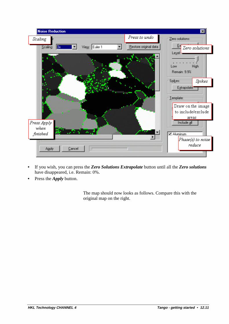
HKL Technology CHANNEL 4 Tango - getting started • 12.11
• If you wish, you can press the Zero Solutions Extrapolate button until all the Zero solutionshave disappeared, i.e. Remain: 0%.
• Press the Apply button.
The map should now looks as follows. Compare this with theoriginal map on the right.
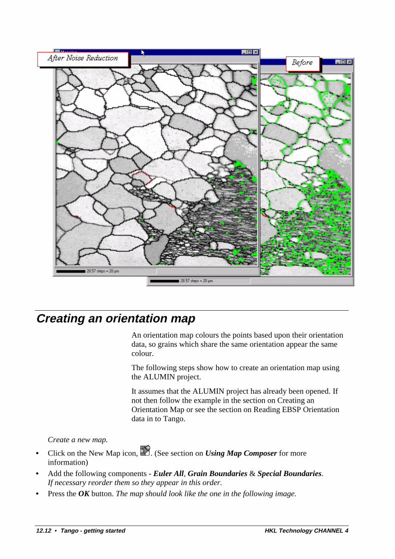
12.12 • Tango - getting started HKL Technology CHANNEL 4
Creating an orientation mapAn orientation map colours the points based upon their orientationdata, so grains which share the same orientation appear the samecolour.
The following steps show how to create an orientation map usingthe ALUMIN project.
It assumes that the ALUMIN project has already been opened. Ifnot then follow the example in the section on Creating anOrientation Map or see the section on Reading EBSP Orientationdata in to Tango.
Create a new map.
• Click on the New Map icon, . (See section on Using Map Composer for moreinformation)
• Add the following components - Euler All, Grain Boundaries & Special Boundaries.If necessary reorder them so they appear in this order.
• Press the OK button. The map should look like the one in the following image.
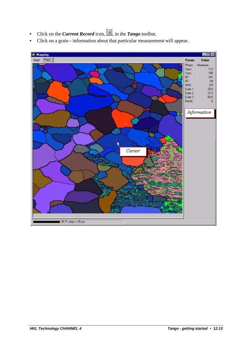
HKL Technology CHANNEL 4 Tango - getting started • 12.13
• Click on the Current Record icon, , in the Tango toolbar.• Click on a grain - information about that particular measurement will appear.
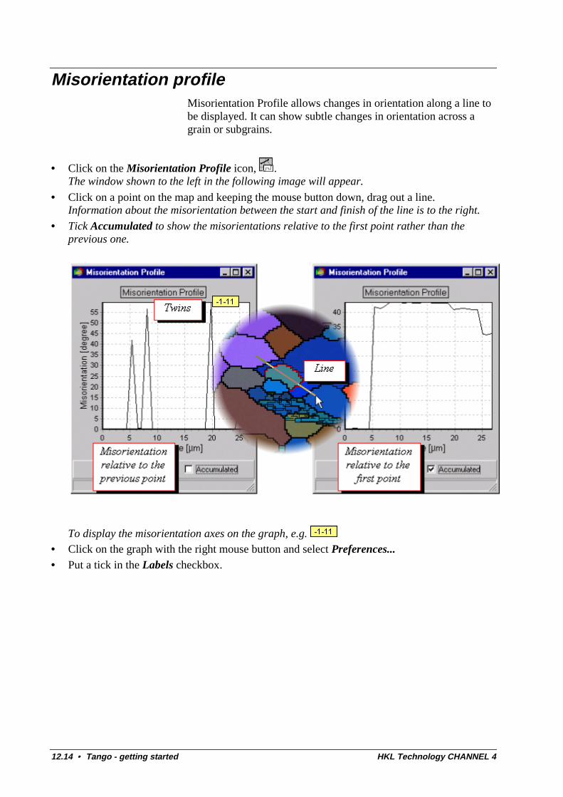
12.14 • Tango - getting started HKL Technology CHANNEL 4
Misorientation profileMisorientation Profile allows changes in orientation along a line tobe displayed. It can show subtle changes in orientation across agrain or subgrains.
• Click on the Misorientation Profile icon, . The window shown to the left in the following image will appear.
• Click on a point on the map and keeping the mouse button down, drag out a line.Information about the misorientation between the start and finish of the line is to the right.
• Tick Accumulated to show the misorientations relative to the first point rather than theprevious one.
To display the misorientation axes on the graph, e.g. • Click on the graph with the right mouse button and select Preferences...• Put a tick in the Labels checkbox.
HKL Technology CHANNEL 4 Tango - getting started • 12.15
Line intercept measurementsThe mean linear intercept method for measuring “grain size” iswell established (e.g. ASTM E112) and has been implemented inTango. A major difference between this implementation and moreconventional ones is that the crystallographic orientation data isbeing used rather than a processed image of an etched specimen.With EBSD data there is no ambiguity about the grains.
Parallel test lines are “drawn” over the map and the points wherethe lines intercept a grain boundary are noted. The mean linearintercept is calculated by adding all the line segments together anddividing by the number of complete grains the test lines passedthrough. Incomplete grains that touch the edges of the map are notincluded. The lines should be at least a grain width apart.
• Select the Edit | Measurement | Line Intercept menu item.The dialog box in the following image will appear.
• Change the values and settings appropriately.• Press the Measure Intercepts button.• Press Close when finished.
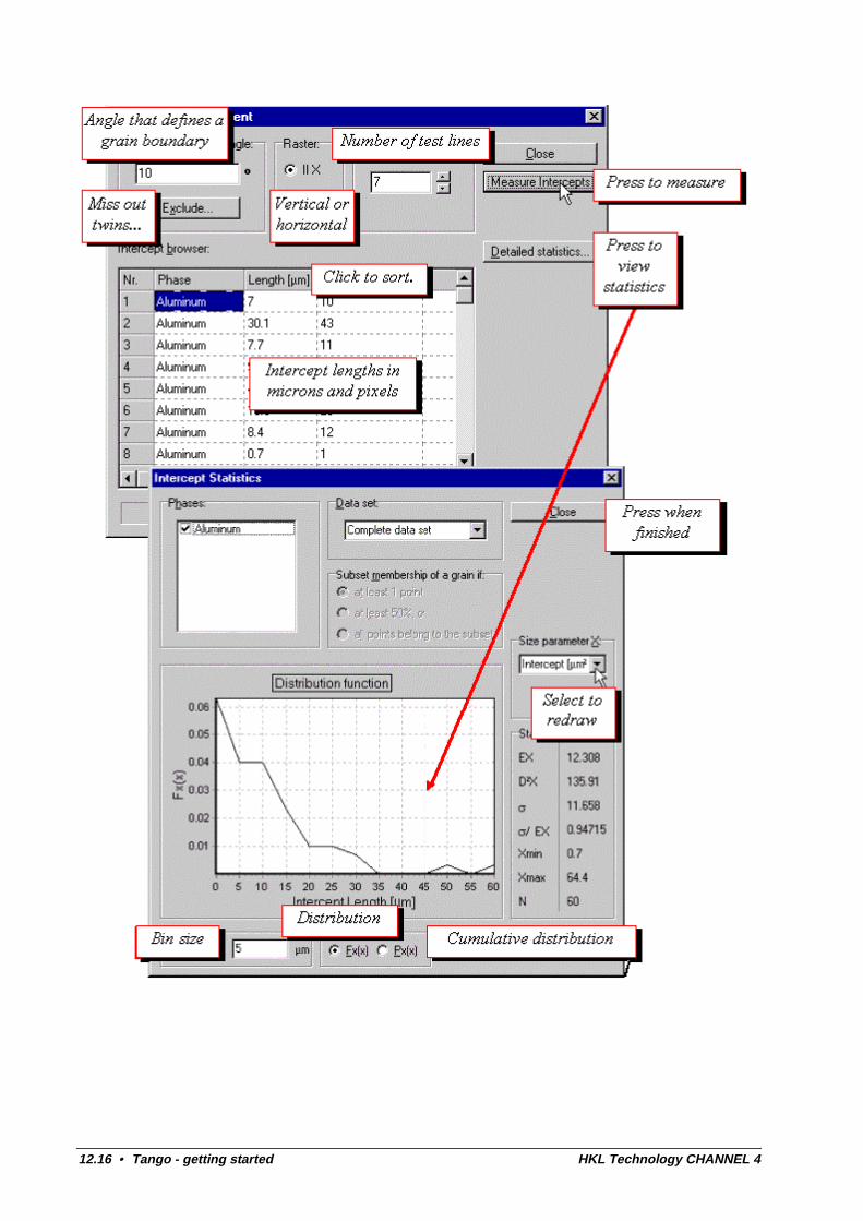
12.16 • Tango - getting started HKL Technology CHANNEL 4
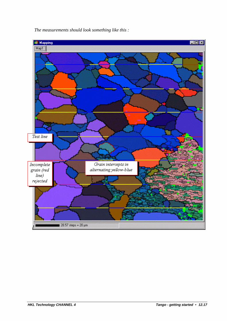
HKL Technology CHANNEL 4 Tango - getting started • 12.17
The measurements should look something like this :
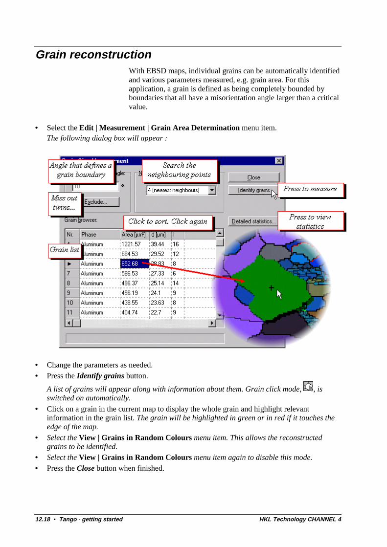
12.18 • Tango - getting started HKL Technology CHANNEL 4
Grain reconstructionWith EBSD maps, individual grains can be automatically identifiedand various parameters measured, e.g. grain area. For thisapplication, a grain is defined as being completely bounded byboundaries that all have a misorientation angle larger than a criticalvalue.
• Select the Edit | Measurement | Grain Area Determination menu item.The following dialog box will appear :
• Change the parameters as needed.• Press the Identify grains button.
A list of grains will appear along with information about them. Grain click mode, , isswitched on automatically.
• Click on a grain in the current map to display the whole grain and highlight relevantinformation in the grain list. The grain will be highlighted in green or in red if it touches theedge of the map.
• Select the View | Grains in Random Colours menu item. This allows the reconstructedgrains to be identified.
• Select the View | Grains in Random Colours menu item again to disable this mode.
• Press the Close button when finished.
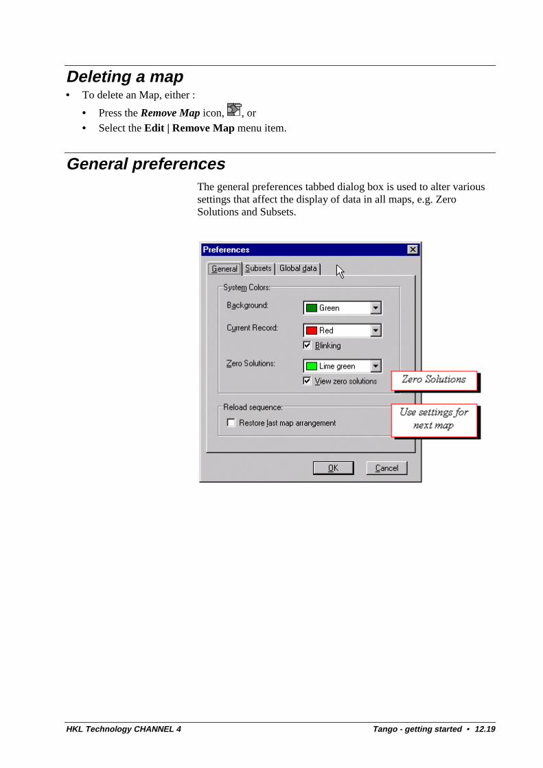
HKL Technology CHANNEL 4 Tango - getting started • 12.19
Deleting a map• To delete an Map, either :
• Press the Remove Map icon, , or• Select the Edit | Remove Map menu item.
General preferencesThe general preferences tabbed dialog box is used to alter varioussettings that affect the display of data in all maps, e.g. ZeroSolutions and Subsets.
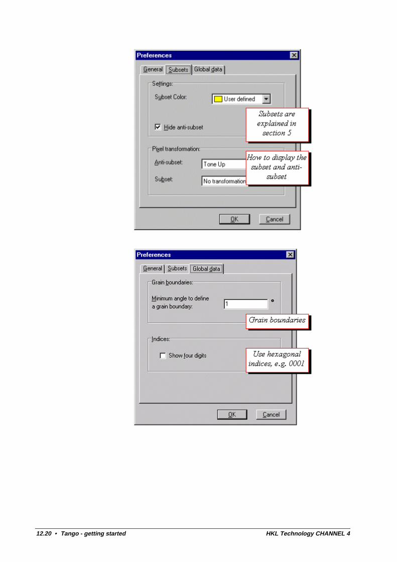
12.20 • Tango - getting started HKL Technology CHANNEL 4
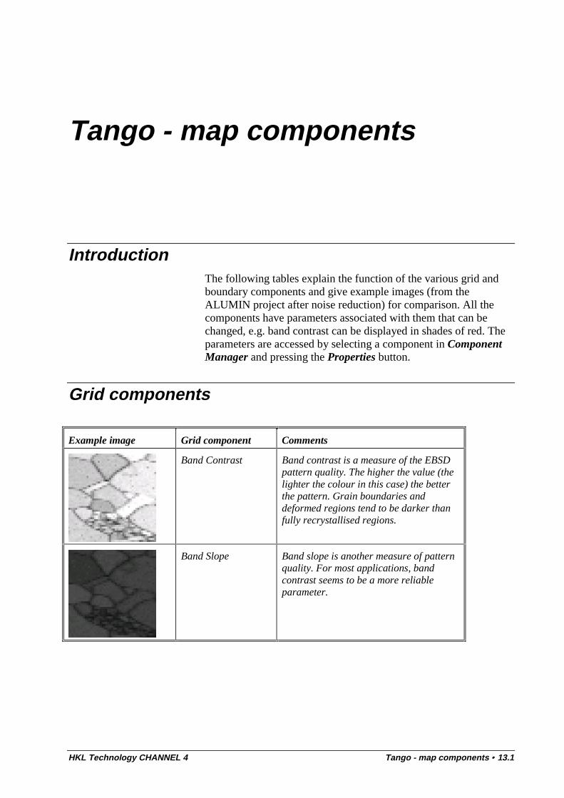
HKL Technology CHANNEL 4 Tango - map components • 13.1
Tango - map components
IntroductionThe following tables explain the function of the various grid andboundary components and give example images (from theALUMIN project after noise reduction) for comparison. All thecomponents have parameters associated with them that can bechanged, e.g. band contrast can be displayed in shades of red. Theparameters are accessed by selecting a component in ComponentManager and pressing the Properties button.
Grid components
Example image Grid component Comments
Band Contrast Band contrast is a measure of the EBSDpattern quality. The higher the value (thelighter the colour in this case) the betterthe pattern. Grain boundaries anddeformed regions tend to be darker thanfully recrystallised regions.
Band Slope Band slope is another measure of patternquality. For most applications, bandcontrast seems to be a more reliableparameter.
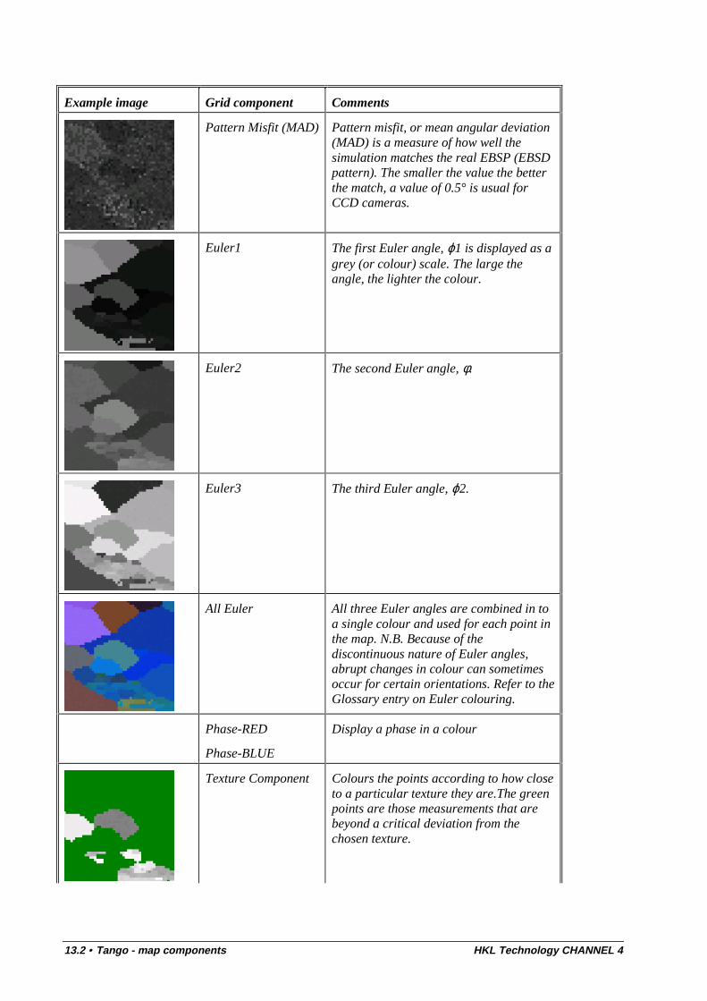
13.2 • Tango - map components HKL Technology CHANNEL 4
Example image Grid component Comments
Pattern Misfit (MAD) Pattern misfit, or mean angular deviation(MAD) is a measure of how well thesimulation matches the real EBSP (EBSDpattern). The smaller the value the betterthe match, a value of 0.5° is usual forCCD cameras.
Euler1 The first Euler angle, ϕ1 is displayed as agrey (or colour) scale. The large theangle, the lighter the colour.
Euler2 The second Euler angle, φ.
Euler3 The third Euler angle, ϕ2.
All Euler All three Euler angles are combined in toa single colour and used for each point inthe map. N.B. Because of thediscontinuous nature of Euler angles,abrupt changes in colour can sometimesoccur for certain orientations. Refer to theGlossary entry on Euler colouring.
Phase-RED
Phase-BLUE
Display a phase in a colour
Texture Component Colours the points according to how closeto a particular texture they are.The greenpoints are those measurements that arebeyond a critical deviation from thechosen texture.
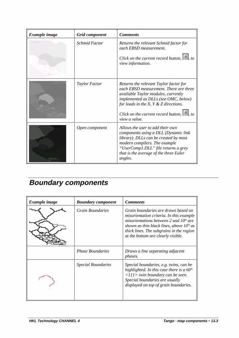
HKL Technology CHANNEL 4 Tango - map components • 13.3
Example image Grid component Comments
Schmid Factor Returns the relevant Schmid factor foreach EBSD measurement.
Click on the current record button, , toview information.
Taylor Factor Returns the relevant Taylor factor foreach EBSD measurement. There are threeavailable Taylor modules, currentlyimplemented as DLLs (see OMC, below)for loads in the X, Y & Z directions.
Click on the current record button, , toview a value.
Open component Allows the user to add their owncomponents using a DLL (Dynamic linklibrary). DLLs can be created by mostmodern compilers. The example“UserComp1.DLL” file returns a greythat is the average of the three Eulerangles.
Boundary components
Example image Boundary component Comments
Grain Boundaries Grain boundaries are drawn based onmisorientation criteria. In this examplemisorientations between 2 and 10° areshown as thin black lines, above 10° asthick lines. The subgrains in the regionat the bottom are clearly visible.
Phase Boundaries Draws a line separating adjacentphases.
Special Boundaries Special boundaries, e.g. twins, can behighlighted. In this case there is a 60°<111> twin boundary can be seen.Special boundaries are usuallydisplayed on top of grain boundaries.

13.4 • Tango - map components HKL Technology CHANNEL 4
Example image Boundary component Comments
CSL Boundaries Coincidence site lattice (CSL)boundaries can also be highlighted,e.g. Σ3. See the Glossary entry formore details.
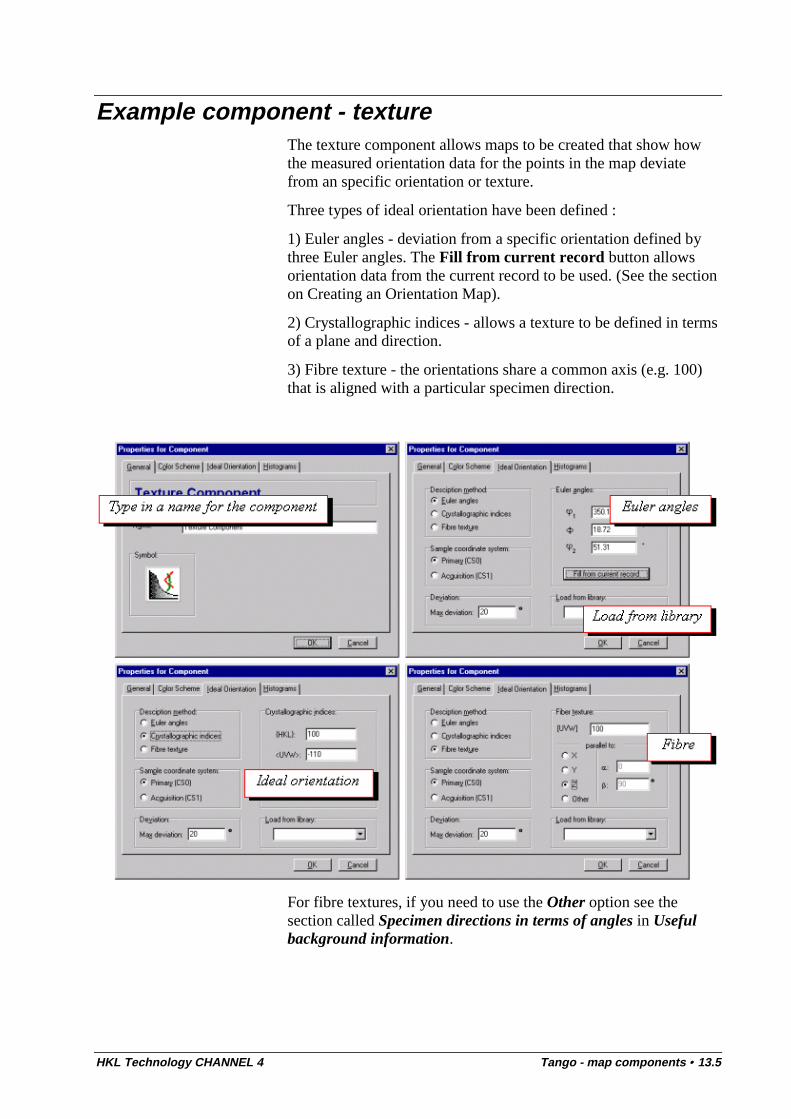
HKL Technology CHANNEL 4 Tango - map components • 13.5
Example component - textureThe texture component allows maps to be created that show howthe measured orientation data for the points in the map deviatefrom an specific orientation or texture.
Three types of ideal orientation have been defined :
1) Euler angles - deviation from a specific orientation defined bythree Euler angles. The Fill from current record button allowsorientation data from the current record to be used. (See the sectionon Creating an Orientation Map).
2) Crystallographic indices - allows a texture to be defined in termsof a plane and direction.
3) Fibre texture - the orientations share a common axis (e.g. 100)that is aligned with a particular specimen direction.
For fibre textures, if you need to use the Other option see thesection called Specimen directions in terms of angles in Usefulbackground information.

HKL Technology CHANNEL 4 Salsa - orientation distribution functions • 14.1
Salsa - orientation distributionfunctions
Salsa - IntroductionSalsa is a statistical tool for generating and displaying (mis-)orientation distribution function, (M)ODF, data from EBSPorientation data. The EBSP data can be obtained from eithermanual or fully automated EBSP measurements using CHANNEL+or from user generated data via an ASCII text file.
Salsa provides a flexible approach to the calculation, display andinterrogation of orientation and misorientation data collectedwithin a crystalline sample. It also allows the data to beinteractively correlated with other microstructural information, e.g.in the new Tango orientation mapping software.

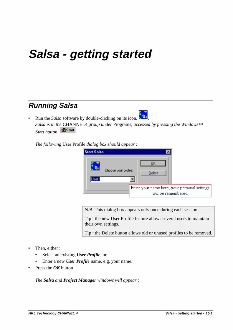
HKL Technology CHANNEL 4 Salsa - getting started • 15.1
Salsa - getting started
Running Salsa
• Run the Salsa software by double-clicking on its icon, .Salsa is in the CHANNEL4 group under Programs, accessed by pressing the Windows™
Start button,
The following User Profile dialog box should appear :
N.B. This dialog box appears only once during each session.
Tip : the new User Profile feature allows several users to maintaintheir own settings.
Tip : the Delete button allows old or unused profiles to be removed.
• Then, either :• Select an existing User Profile, or• Enter a new User Profile name, e.g. your name.
• Press the OK button
The Salsa and Project Manager windows will appear :
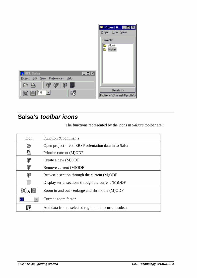
15.2 • Salsa - getting started HKL Technology CHANNEL 4
Salsa’s toolbar iconsThe functions represented by the icons in Salsa’s toolbar are :
Icon Function & comments
Open project - read EBSP orientation data in to Salsa
Printthe current (M)ODF
Create a new (M)ODF
Remove current (M)ODF
Browse a section through the current (M)ODF
Display serial sections through the current (M)ODF
& Zoom in and out - enlarge and shrink the (M)ODF
Current zoom factor
Add data from a selected region to the current subset
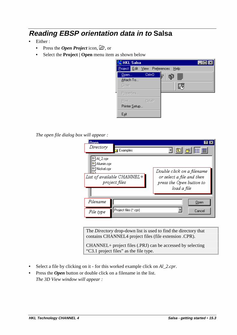
HKL Technology CHANNEL 4 Salsa - getting started • 15.3
Reading EBSP orientation data in to Salsa• Either :
• Press the Open Project icon, , or• Select the Project | Open menu item as shown below
The open file dialog box will appear :
The Directory drop-down list is used to find the directory thatcontains CHANNEL4 project files (file extension .CPR).
CHANNEL+ project files (.PRJ) can be accessed by selecting“C3.1 project files” as the file type.
• Select a file by clicking on it - for this worked example click on Al_2.cpr.• Press the Open button or double click on a filename in the list.
The 3D View window will appear :
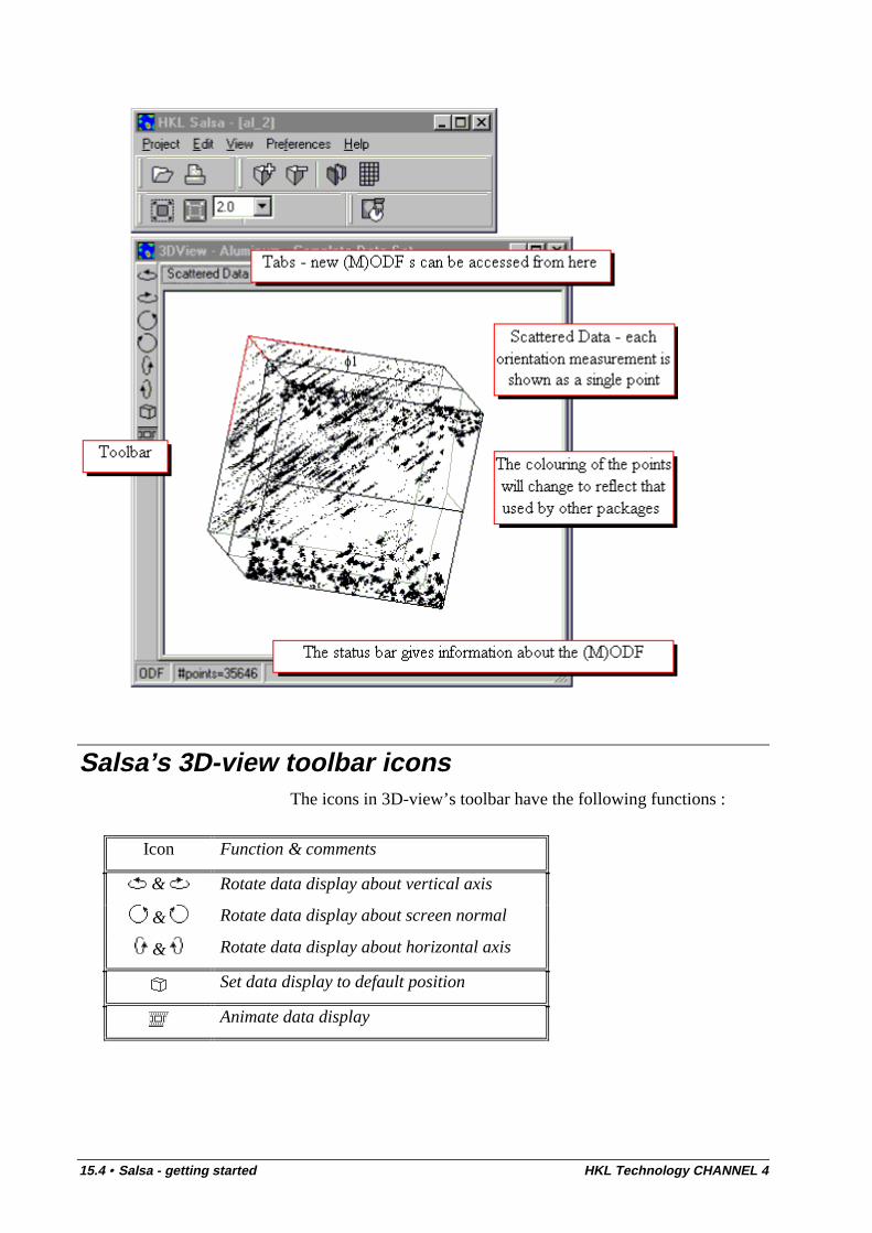
15.4 • Salsa - getting started HKL Technology CHANNEL 4
Salsa’s 3D-view toolbar iconsThe icons in 3D-view’s toolbar have the following functions :
Icon Function & comments
& Rotate data display about vertical axis
& Rotate data display about screen normal
& Rotate data display about horizontal axis
Set data display to default position
Animate data display
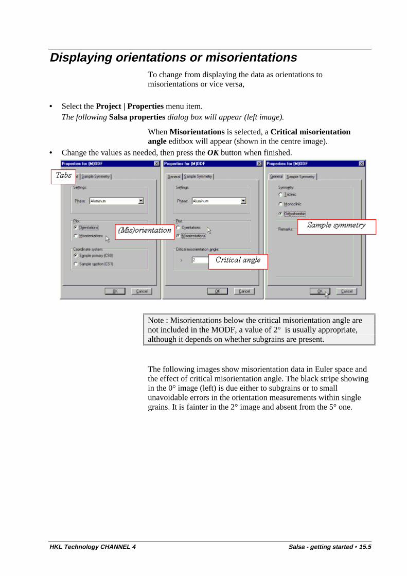
HKL Technology CHANNEL 4 Salsa - getting started • 15.5
Displaying orientations or misorientationsTo change from displaying the data as orientations tomisorientations or vice versa,
• Select the Project | Properties menu item.The following Salsa properties dialog box will appear (left image).
When Misorientations is selected, a Critical misorientationangle editbox will appear (shown in the centre image).
• Change the values as needed, then press the OK button when finished.
Note : Misorientations below the critical misorientation angle arenot included in the MODF, a value of 2° is usually appropriate,although it depends on whether subgrains are present.
The following images show misorientation data in Euler space andthe effect of critical misorientation angle. The black stripe showingin the 0° image (left) is due either to subgrains or to smallunavoidable errors in the orientation measurements within singlegrains. It is fainter in the 2° image and absent from the 5° one.
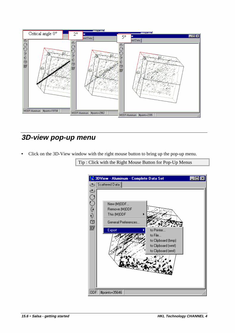
15.6 • Salsa - getting started HKL Technology CHANNEL 4
3D-view pop-up menu
• Click on the 3D-View window with the right mouse button to bring up the pop-up menu.
Tip : Click with the Right Mouse Button for Pop-Up Menus

HKL Technology CHANNEL 4 Salsa - getting started • 15.7
There are five main menu items :
New (M)ODF… to calculate a new (M)ODF
Remove (M)ODF
This (M)ODF to recalculate the current (M)ODF
Preferences... which is explained below.
Export to Printer, File, Clipboard (as Windows bitmap or (enhanced) graphics metafile)
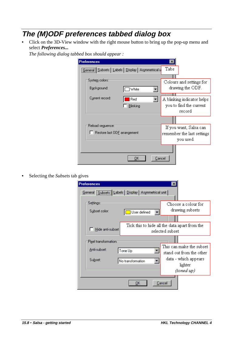
15.8 • Salsa - getting started HKL Technology CHANNEL 4
The (M)ODF preferences tabbed dialog box• Click on the 3D-View window with the right mouse button to bring up the pop-up menu and
select Preferences...The following dialog tabbed box should appear :
• Selecting the Subsets tab gives
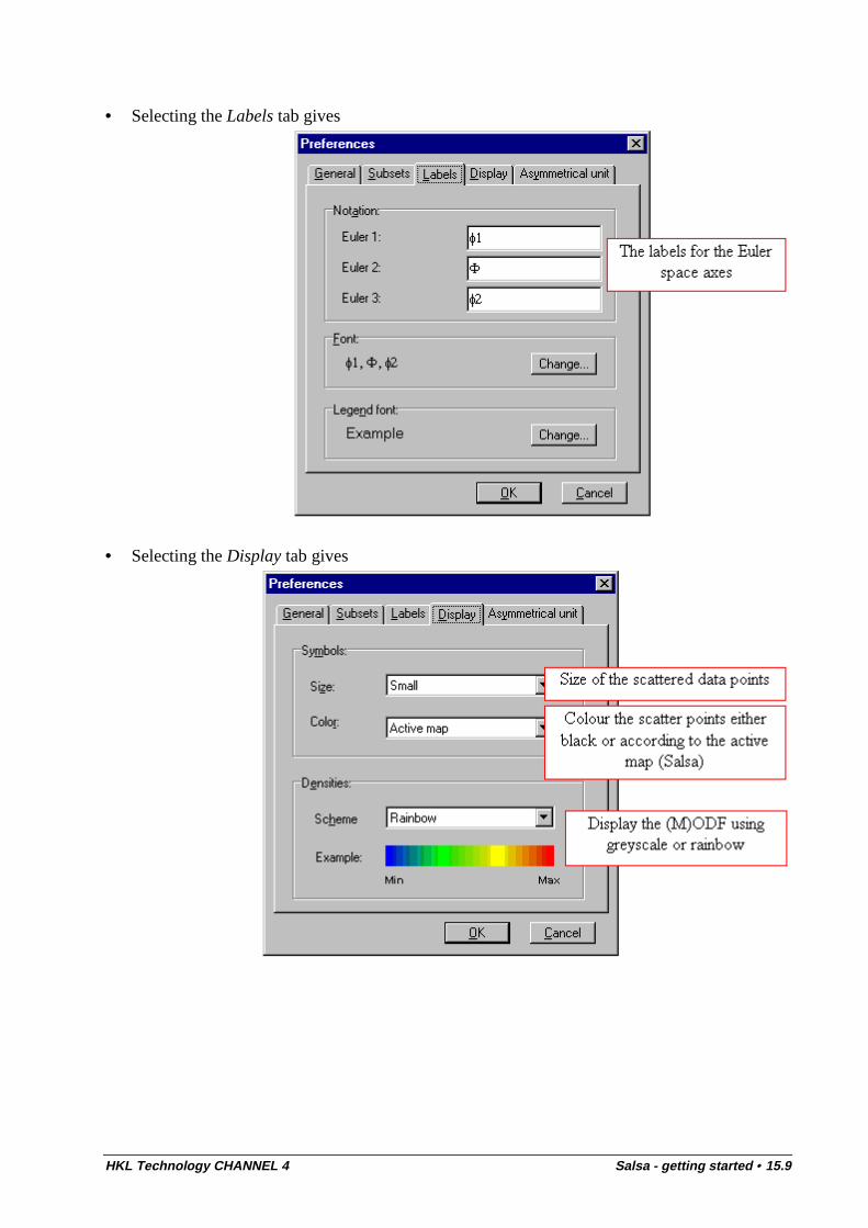
HKL Technology CHANNEL 4 Salsa - getting started • 15.9
• Selecting the Labels tab gives
• Selecting the Display tab gives
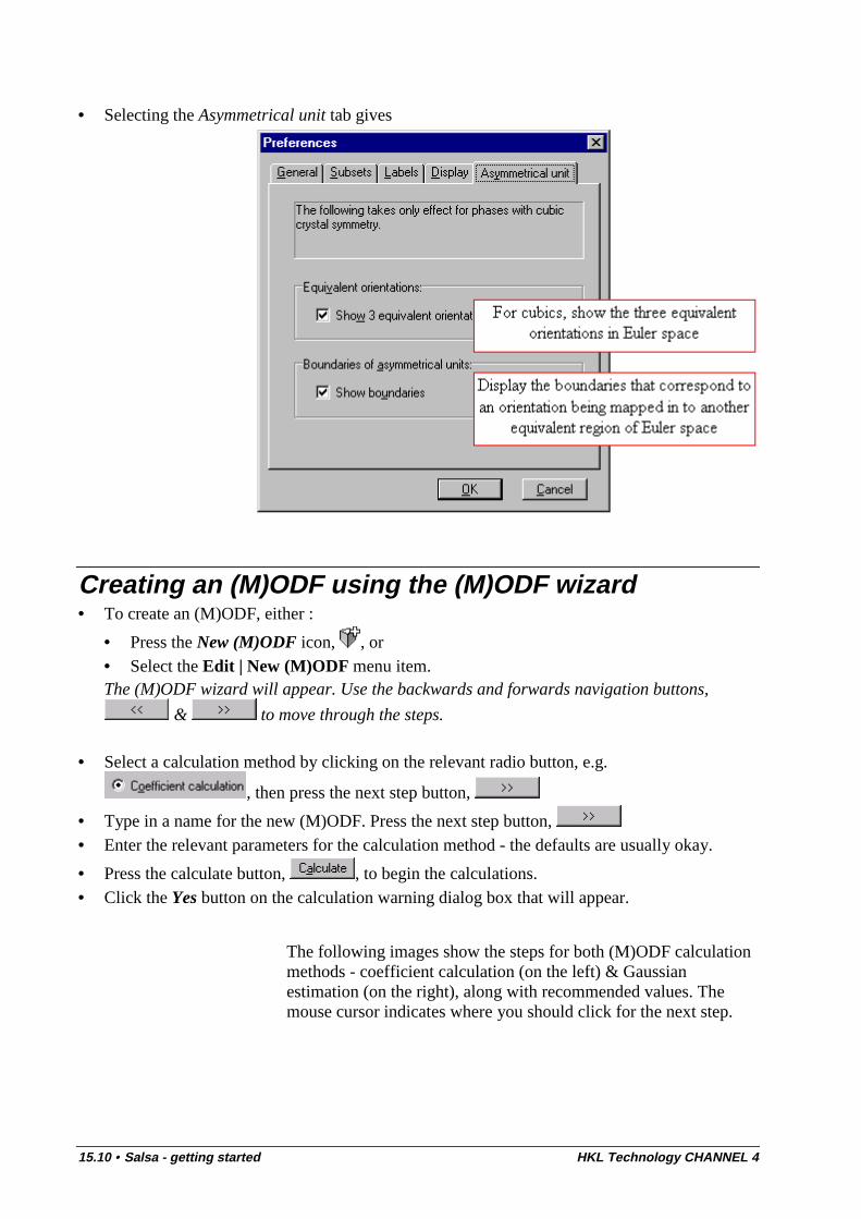
15.10 • Salsa - getting started HKL Technology CHANNEL 4
• Selecting the Asymmetrical unit tab gives
Creating an (M)ODF using the (M)ODF wizard• To create an (M)ODF, either :
• Press the New (M)ODF icon, , or• Select the Edit | New (M)ODF menu item.The (M)ODF wizard will appear. Use the backwards and forwards navigation buttons,
& to move through the steps.
• Select a calculation method by clicking on the relevant radio button, e.g.
, then press the next step button,
• Type in a name for the new (M)ODF. Press the next step button, • Enter the relevant parameters for the calculation method - the defaults are usually okay.
• Press the calculate button, , to begin the calculations.• Click the Yes button on the calculation warning dialog box that will appear.
The following images show the steps for both (M)ODF calculationmethods - coefficient calculation (on the left) & Gaussianestimation (on the right), along with recommended values. Themouse cursor indicates where you should click for the next step.
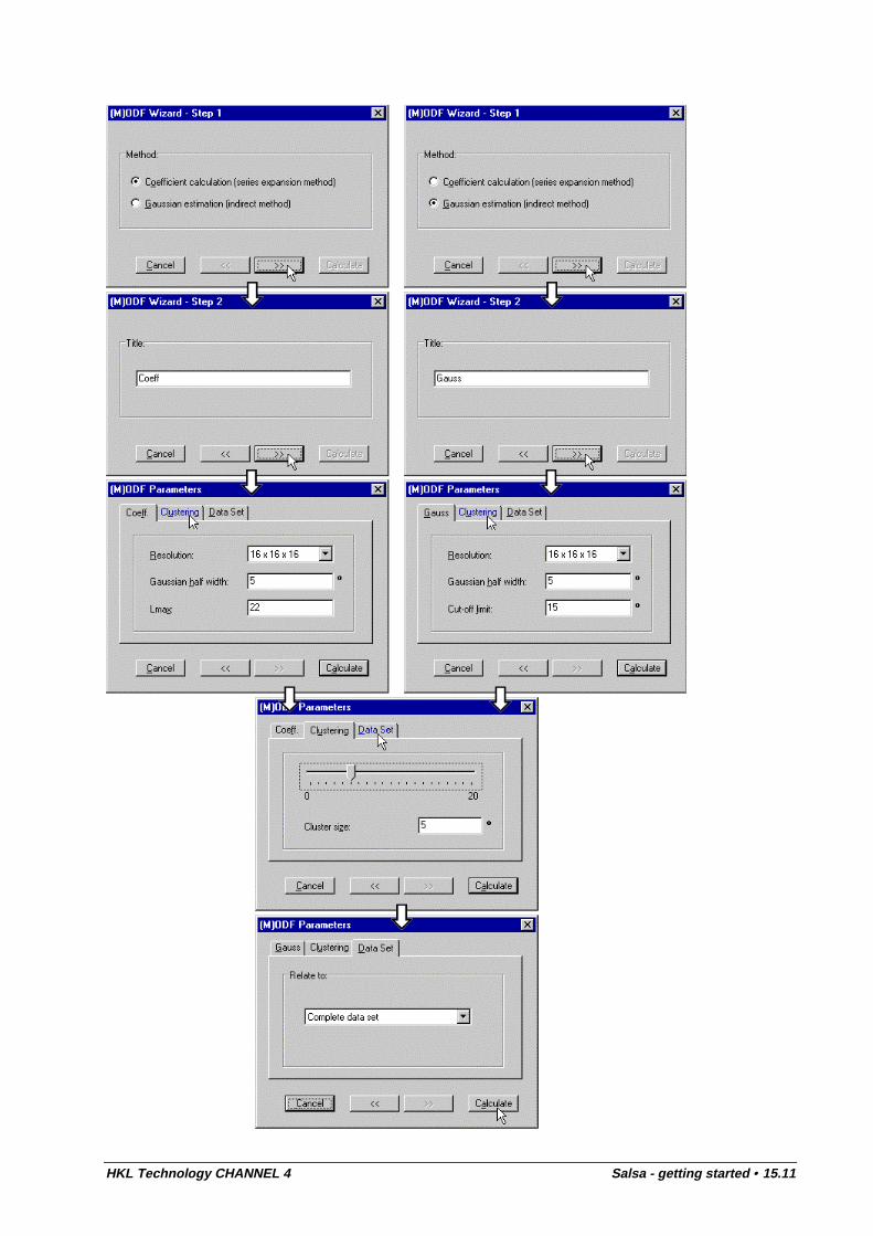
HKL Technology CHANNEL 4 Salsa - getting started • 15.11
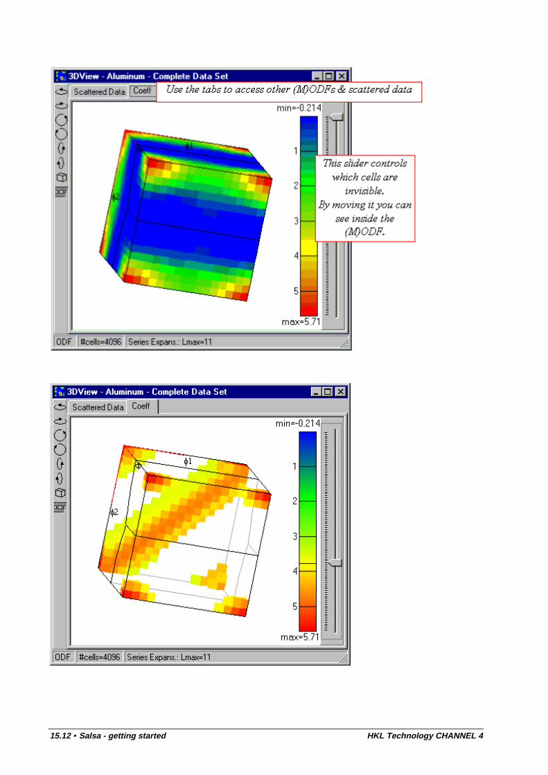
15.12 • Salsa - getting started HKL Technology CHANNEL 4
HKL Technology CHANNEL 4 Salsa - getting started • 15.13
Deleting an (M)ODF• To delete an (M)ODF, either :
• Press the Remove (M)ODF icon, , or• Select the Edit | Remove (M)ODF menu item.
Altering the (M)ODF method and parametersTo change the (M)ODFs method and parameters,
• Select the Edit | This (M)ODF | (M)ODF wizard menu item and follow the wizard steps asexplained in the previous section.
Reviewing the (M)ODF parametersTo reviewthe (M)ODFa parameters,
• Select the Edit | This (M)ODF | Parameters menu item.• Pressing the Calculate button will cause the (M)ODF to be recalculated.
Browsing a section through the (M)ODFTo browse a section through the (M)ODF, either :
• Press the Section Browser icon, , or• Select the View | Browser menu item.
The following Section Browser window will appear and theposition of the section will be shown on the (M)ODF image in red.The function of the icons is shown below.
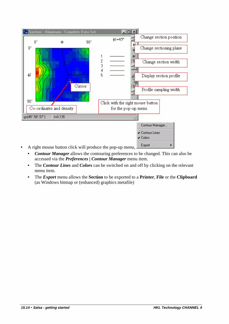
15.14 • Salsa - getting started HKL Technology CHANNEL 4
• A right mouse button click will produce the pop-up menu, • Contour Manager allows the contouring preferences to be changed. This can also be
accessed via the Preferences | Contour Manager menu item.
• The Contour Lines and Colors can be switched on and off by clicking on the relevantmenu item.
• The Export menu allows the Section to be exported to a Printer, File or the Clipboard(as Windows bitmap or (enhanced) graphics metafile)
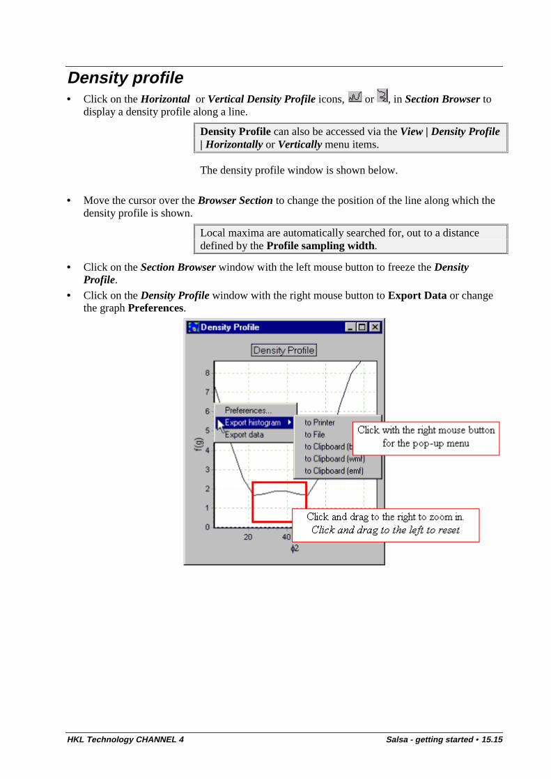
HKL Technology CHANNEL 4 Salsa - getting started • 15.15
Density profile• Click on the Horizontal or Vertical Density Profile icons, or , in Section Browser to
display a density profile along a line.
Density Profile can also be accessed via the View | Density Profile| Horizontally or Vertically menu items.
The density profile window is shown below.
• Move the cursor over the Browser Section to change the position of the line along which thedensity profile is shown.
Local maxima are automatically searched for, out to a distancedefined by the Profile sampling width.
• Click on the Section Browser window with the left mouse button to freeze the DensityProfile.
• Click on the Density Profile window with the right mouse button to Export Data or changethe graph Preferences.
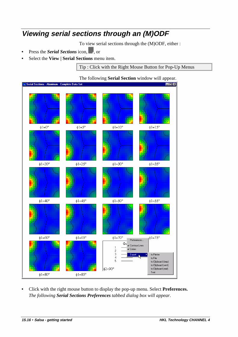
15.16 • Salsa - getting started HKL Technology CHANNEL 4
Viewing serial sections through an (M)ODFTo view serial sections through the (M)ODF, either :
• Press the Serial Sections icon, , or• Select the View | Serial Sections menu item.
Tip : Click with the Right Mouse Button for Pop-Up Menus
The following Serial Section window will appear.
• Click with the right mouse button to display the pop-up menu. Select Preferences.The following Serial Sections Preferences tabbed dialog box will appear.
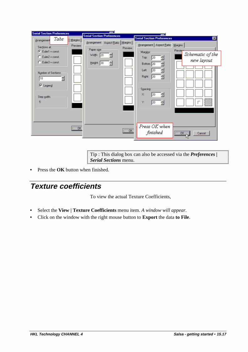
HKL Technology CHANNEL 4 Salsa - getting started • 15.17
Tip : This dialog box can also be accessed via the Preferences |Serial Sections menu.
• Press the OK button when finished.
Texture coefficientsTo view the actual Texture Coefficients,
• Select the View | Texture Coefficients menu item. A window will appear.
• Click on the window with the right mouse button to Export the data to File.
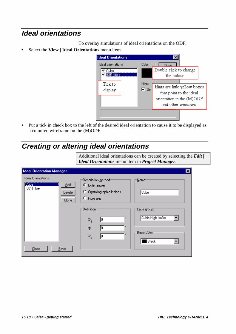
15.18 • Salsa - getting started HKL Technology CHANNEL 4
Ideal orientationsTo overlay simulations of ideal orientations on the ODF,
• Select the View | Ideal Orientations menu item.
• Put a tick in check box to the left of the desired ideal orientation to cause it to be displayed asa coloured wireframe on the (M)ODF.
Creating or altering ideal orientationsAdditional ideal orientations can be created by selecting the Edit |Ideal Orientations menu item in Project Manager.
HKL Technology CHANNEL 4 Salsa - introduction to ODF calculations • 16.1
Salsa - introduction to ODFcalculations
IntroductionThe Orientation Distribution Function (ODF) is a means ofrepresenting preferred orientations for materials. It is a fourdimensional object - the four dimensions being the three Eulerangles and a density value corresponding to how many strongly aparticular orientation appears. This strength is expressed as a ratioto that expected for a completely random distribution oforientations.
The ODF approach to texture measurements has many strengthsand a few weaknesses (e.g. there is no intuitive connection betweenEuler space and specimen (i.e. physical) space). There is also a vastreservoir of experience and experimental X-raydiffraction data,much of it in the form of ODFs, that can be tapped in to.
EBSD orientation measurements are complete (unlike X-ray whichusually measures the distribution of poles) and can also be relatedto microstructure (via Tango) and expressed as misorientationswhich can also be plotted in Euler space using Salsa. Neither ofthese approaches were practical using conventional X-raydiffraction and it is clear that EBSD texture measurements can rivalthose made by X-ray methods in both speed and accuracy.
For an in depth explanation of ODFs, the reader is referred to H.-J.Bunge’s book Texture Analysis in Materials Science, (CuvillerVerlag, 1993, ISBN 3-928815-18-4).
16.2 • Salsa - introduction to ODF calculations HKL Technology CHANNEL 4
The result of an (M)ODF calculationThe result of an (M)ODF calculation is a three-dimensional arrayof densities, expressed as multiples of the random orientationdistribution function. Each array item represents a cell with acertain width. The parameter Resolution which has to be specifiedin the first tab of the (M)ODF Parameters dialog box determinesthe resolution with which the (M)ODF is calculated.
Note that the calculation routines operate internally with cellwidths chosen so that the number of cells in each direction ϕ1,Φ,and ϕ2 gives a power of 2 (2, 4, 8, 16, etc.).
The larger the values of Resolution, the longer the time taken forthe calculations. A value near 8x8x8 is a good compromisebetween accuracy and calculation speed.
Equivalence of orientation andmisorientationIn the calculations, both orientations and misorientations areconsidered as sets of Euler angles. Therefore, no difference is mademathematically between orientations and misorientations, neitherfor their calculation nor for the displaying of results in Euler space
Determination of misorientation
In the Salsa software the misorientation gijm
is calculated between
the orientation gi of a grid point and its nearest neighbour g j (two
per point, one to the right and one below) using the followingequation:
g g gijm
i j= −1.
The critical misorientation angle (accessed via the Project |Properties menu and selecting the ‘Misorientation’ radio button) isused to filter out orientation noise. See the Glossary entry for moreinformation.
Coordinate systemsNote that there are two coordinate systems the data can refer to,namely the sample coordinate system CS0 (usually expressed asrolling, transversal, and normal direction) and the coordinatesystem of the acquisition surface CS1 . If these two coordinatesystems are not identical, it is of major importance for the resultsobtained with Salsa to choose the correct coordinate system. This
HKL Technology CHANNEL 4 Salsa - introduction to ODF calculations • 16.3
can be accessed by the Project | Properties menu and selecting therelevant radio button under Coordinate System.
This problem is only relevant for the orientation distributionfunction, since a misorientation is basically the rotation betweenthe crystal coordinate systems ( CS i2 and CS j2 ) of neighbouring
measurements. It is thus not influenced by the choice of thereference coordinate system.
Calculation methodsTwo different calculation methods can be applied:
1) the Gaussian kernel estimation and
2) the Series expansion method.
Common to both methods is, that each measured point in the Eulerspace is approached by a Gaussian distibution around the actualEuler position (Bunge 1985a) with a given half scatter width Ψ0
(The half scatter width is here considered to be the angular distancefrom the peak to where the probability has decreased by a factor of1/e). Furthermore, a weight is assigned to each point. This weightis typically set to 1/N (N: number of measurements), except whenthe data is clustered (see next section).
The (M)ODF calculation is usually a time consuming process. Themore data points that have to have to be considered, the longer thetime taken for calculation. Clustering is used to speed up thecalculations. See the Glossary entry for more information.
Gaussian Kernel EstimationAs already mentioned, each point in the Euler space is approachedby a three-dimensional Gaussian distribution function with a halfscatter width Ψ0 and a weight Wi . Additionally, a cut-off of theGaussian distribution function can be defined. Outside this cut-off,measured from the center of the Gaussian, its probability is set tozero. (Note that at a distance of 3 times the half scatter width Ψ0
from the center of a Gaussian distribution function, the probabilityhas decreased by a factor of 0.0001). Since the Gaussian kernelestimation is basically a summation of the single distributions, thechoice of the cut-off also influences the computing time.
The a priori result of the Gaussian kernel estimation is a threedimensional distribution function whose ‘4D-volume’ is 1 (unity).This is much the manner as a one dimensional Gaussiandistribution can be normalised to unity by integrating the areaunder the curve and dividing by the number you first thought of.
16.4 • Salsa - introduction to ODF calculations HKL Technology CHANNEL 4
In order to obtain the densities as multiples of the randomdistribution function, such a random distribution function isinternally created by the software (whose “4D-volume” is againunity). The density of each single cell in the Euler space is thencorrected simply by dividing the value of the estimation by thevalue obtained from the random distribution.
When calculating the random distribution function, it is assumedthat the probability in this case is (Bunge, 1993, Texture Analysisin Materials Science, ISBN 3-928815-18-4)
P( ) sin( )ϕ ϕ1 2Φ Φ∝ (1)
Series Expansion MethodThe principle of the series expansion method consists of two steps:
Calculation of the so-called texture coefficients (which arecoefficients of the series expansion method)
Calculation of the (M)ODF out of the texture coefficients
The calculation of the texture coefficients requires again a halfscatter width of the Gaussian distribution function whichapproaches each data point in the Euler space. Unlike the Gaussiankernel estimation method, no cut-off is needed. This becomesapparent if one looks at the equation for the calculation of thecoefficients C mn
1 :
( )
CN
l l
T glmn
lmn
ii l
N
=
−
− −
+
− −
⋅=∑1 4
1
4
14
202 2
02
02
exp exp
exp
( )
Ψ Ψ
Ψ (2)
N : number of data points
Ψ0 : Gaussian half scatter width (to be specified by user)
l : Highest harmonic (to be specified by user)
T : generalised spherical harmonic function
m, n : Indices refering to crystal (m) and sample symmetry (n).
The highest harmonic l can be understood as a upper cut-off of theseries expansion. The lower this value, the less accurate the result.The large this value, the longer the calculation time. Appropriatevalues range between l=11 and l=22.
HKL Technology CHANNEL 4 Salsa - introduction to ODF calculations • 16.5
The generalised spherical harmonics T are determined by thesoftware. They depend upon the crystal and the sample symmetry.Since all HKL products assume always triclinic sample symmetry,the parameter n is internally accordingly defined and no userchoice of n is provided in the software. This is also the reason forthe fact that the Euler space is always plotted over the entire range(e.g. cubic: 360°, 90°, 90°).
Recommended ParametersThe following recommendations are mostly based on limitedpersonal experience. They should not be regarded as definite rules.Some experimentation with the parameters will be necessary.
Parameter Gaussian Kernel Estimation Series Expansion Method
Clustering <5° <5°Resolution 16 x16 x16 16 x16 x16Half Scatter Width 2° to 5°Cut-off 2 to3 x Half scatter width -Highest harmonic - 11 to 22
Comparison of the Calculation MethodsA limited comparison of the two methods has been carried out forseveral sets of data. The results were qualitatively the same withsimilar surfaces appearing, the relative intensities tended to differthough.
However, since these two algorithms are completely different intheir approaches, one must expect different results, at leastquantitatively. It is also difficult to carry out a meaningfulcomparison, since the parameters used are different and not reallycompatible.
The first point of major importance is that the results of theGaussian kernel estimation have to be normalised to multiples of a“random distribution”. As can be seen from equation (2), this“random distribution” approaches zero at very low values of thesecond Euler angle Φ and the values become unrealistic (asΘ Θ→ → ∞0 1, sin( ) ). As a consequence, the Gaussian kernelestimation seems to overestimate the densities, especially for lowvalues of the second Euler angle Φ.
In the series expansion method no such extra normalisation isneeded, the “inventors” of this method claim that the results arenormalised with respect to a random distribution per se. Thismethod seems therefore to have some advantages over the other,and is more often used in literature. A disadvantage is that it can

16.6 • Salsa - introduction to ODF calculations HKL Technology CHANNEL 4
give nonsensical negative values (seen as obviously “wrong”colours in the ODF).

HKL Technology CHANNEL 4 Subsets • 17.1
Subsets
Subsets - introductionSubsets are a core concept within the CHANNEL suite ofprograms. They allow the user to select data on a wide variety ofcriteria and to manipulate and display this data separately, i.e. as asubset of all the data.
The user may want to work only with data from a particular groupof grains near a crack or to display data for grains that are within10° of a <100> fibre texture parallel to the specimens X-axis or tolocate the few cube orientated grains in an assemblage that aremainly random in orientation.
All of these can be achieved with relative ease using subsets.
Each of the packages can create different sorts of subsets which areaccessible by the other packages. Project Manger can also combinethe subsets together in different ways, e.g. show data in subset1 butnot in subset2.
The data that is not in the current subset is known as the anti-subsetand it can either not be displayed at all or it can be displayed as adifferent colour. By default the anti-subset will be toned up(colours will appear lighter); this behaviour can be changed.
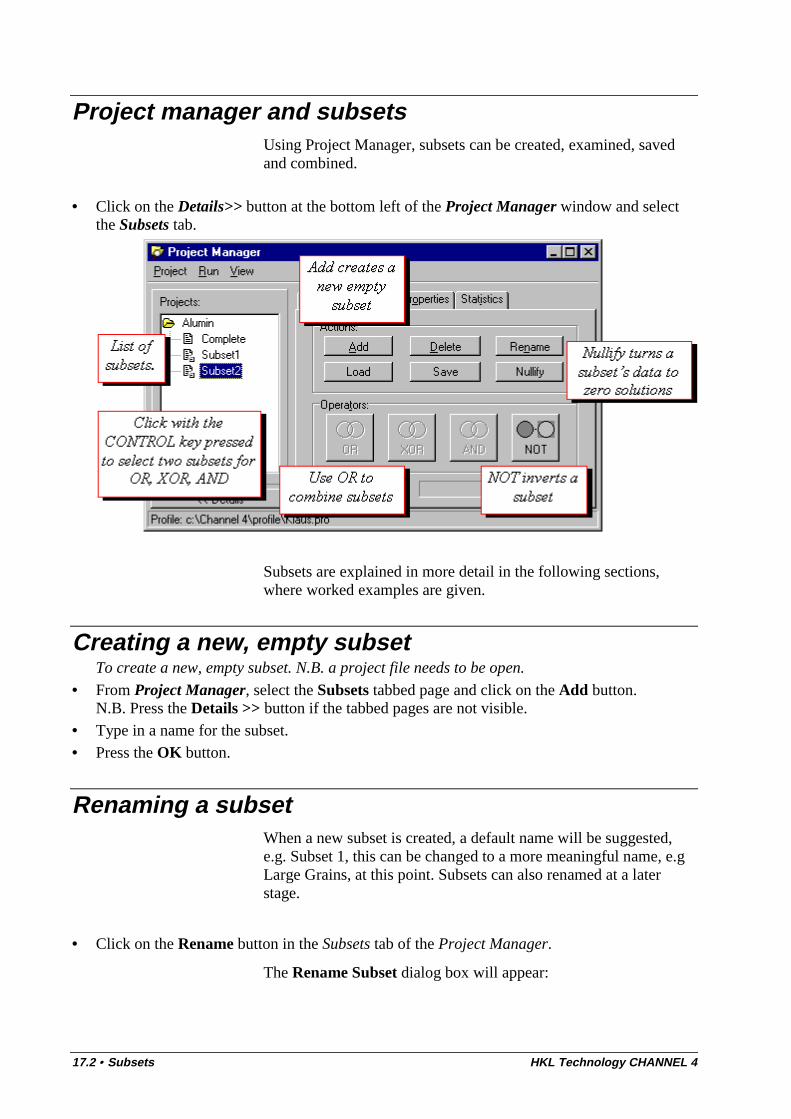
17.2 • Subsets HKL Technology CHANNEL 4
Project manager and subsetsUsing Project Manager, subsets can be created, examined, savedand combined.
• Click on the Details>> button at the bottom left of the Project Manager window and selectthe Subsets tab.
Subsets are explained in more detail in the following sections,where worked examples are given.
Creating a new, empty subsetTo create a new, empty subset. N.B. a project file needs to be open.
• From Project Manager, select the Subsets tabbed page and click on the Add button.N.B. Press the Details >> button if the tabbed pages are not visible.
• Type in a name for the subset.• Press the OK button.
Renaming a subsetWhen a new subset is created, a default name will be suggested,e.g. Subset 1, this can be changed to a more meaningful name, e.gLarge Grains, at this point. Subsets can also renamed at a laterstage.
• Click on the Rename button in the Subsets tab of the Project Manager.
The Rename Subset dialog box will appear:
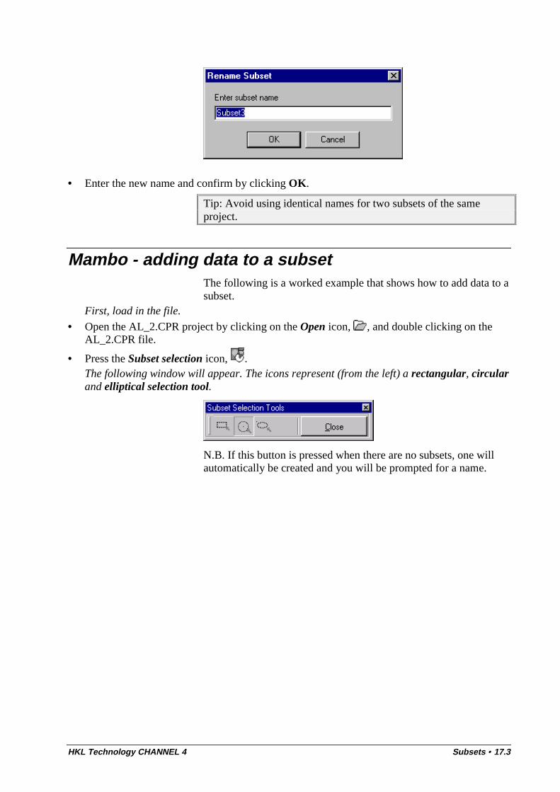
HKL Technology CHANNEL 4 Subsets • 17.3
• Enter the new name and confirm by clicking OK.
Tip: Avoid using identical names for two subsets of the sameproject.
Mambo - adding data to a subsetThe following is a worked example that shows how to add data to asubset.
First, load in the file.
• Open the AL_2.CPR project by clicking on the Open icon, , and double clicking on theAL_2.CPR file.
• Press the Subset selection icon, .The following window will appear. The icons represent (from the left) a rectangular, circularand elliptical selection tool.
N.B. If this button is pressed when there are no subsets, one willautomatically be created and you will be prompted for a name.
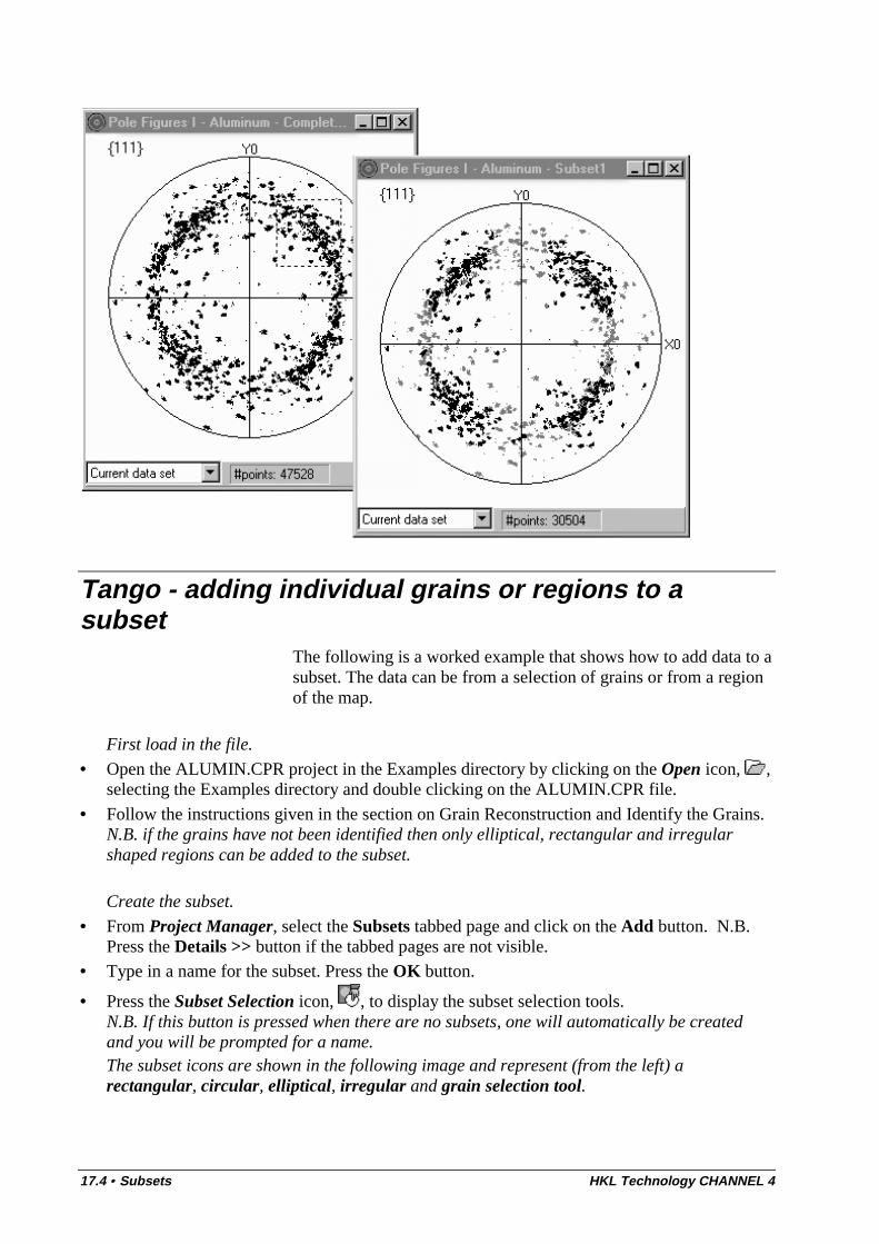
17.4 • Subsets HKL Technology CHANNEL 4
Tango - adding individual grains or regions to asubset
The following is a worked example that shows how to add data to asubset. The data can be from a selection of grains or from a regionof the map.
First load in the file.
• Open the ALUMIN.CPR project in the Examples directory by clicking on the Open icon, ,selecting the Examples directory and double clicking on the ALUMIN.CPR file.
• Follow the instructions given in the section on Grain Reconstruction and Identify the Grains.N.B. if the grains have not been identified then only elliptical, rectangular and irregularshaped regions can be added to the subset.
Create the subset.
• From Project Manager, select the Subsets tabbed page and click on the Add button. N.B.Press the Details >> button if the tabbed pages are not visible.
• Type in a name for the subset. Press the OK button.
• Press the Subset Selection icon, , to display the subset selection tools.N.B. If this button is pressed when there are no subsets, one will automatically be createdand you will be prompted for a name.The subset icons are shown in the following image and represent (from the left) arectangular, circular, elliptical, irregular and grain selection tool.
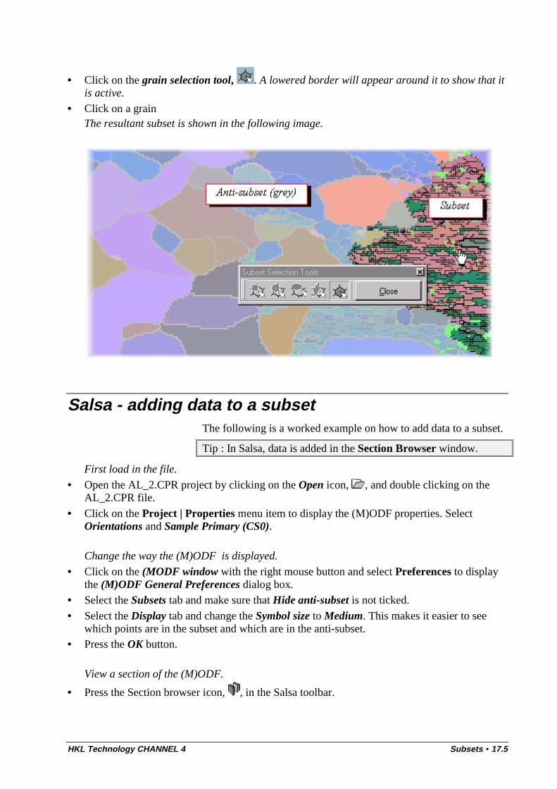
HKL Technology CHANNEL 4 Subsets • 17.5
• Click on the grain selection tool, . A lowered border will appear around it to show that itis active.
• Click on a grainThe resultant subset is shown in the following image.
Salsa - adding data to a subsetThe following is a worked example on how to add data to a subset.
Tip : In Salsa, data is added in the Section Browser window.
First load in the file.
• Open the AL_2.CPR project by clicking on the Open icon, , and double clicking on theAL_2.CPR file.
• Click on the Project | Properties menu item to display the (M)ODF properties. SelectOrientations and Sample Primary (CS0).
Change the way the (M)ODF is displayed.
• Click on the (MODF window with the right mouse button and select Preferences to displaythe (M)ODF General Preferences dialog box.
• Select the Subsets tab and make sure that Hide anti-subset is not ticked.
• Select the Display tab and change the Symbol size to Medium. This makes it easier to seewhich points are in the subset and which are in the anti-subset.
• Press the OK button.
View a section of the (M)ODF.
• Press the Section browser icon, , in the Salsa toolbar.
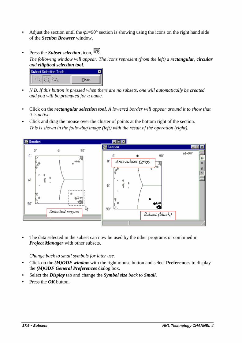
17.6 • Subsets HKL Technology CHANNEL 4
• Adjust the section until the φ1=90° section is showing using the icons on the right hand sideof the Section Browser window.
• Press the Subset selection ,icon, . The following window will appear. The icons represent (from the left) a rectangular, circularand elliptical selection tool.
• N.B. If this button is pressed when there are no subsets, one will automatically be created
and you will be prompted for a name.
• Click on the rectangular selection tool. A lowered border will appear around it to show thatit is active.
• Click and drag the mouse over the cluster of points at the bottom right of the section. This is shown in the following image (left) with the result of the operation (right).
• The data selected in the subset can now be used by the other programs or combined inProject Manager with other subsets.
Change back to small symbols for later use.
• Click on the (M)ODF window with the right mouse button and select Preferences to displaythe (M)ODF General Preferences dialog box.
• Select the Display tab and change the Symbol size back to Small.• Press the OK button.
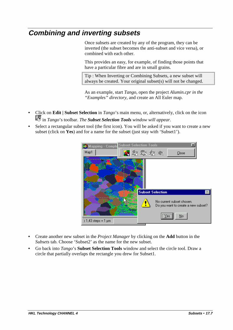
HKL Technology CHANNEL 4 Subsets • 17.7
Combining and inverting subsetsOnce subsets are created by any of the program, they can beinverted (the subset becomes the anti-subset and vice versa), orcombined with each other.
This provides an easy, for example, of finding those points thathave a particular fibre and are in small grains.
Tip : When Inverting or Combining Subsets, a new subset willalways be created. Your original subset(s) will not be changed.
As an example, start Tango, open the project Alumin.cpr in the“Examples” directory, and create an All Euler map.
• Click on Edit | Subset Selection in Tango’s main menu, or, alternatively, click on the icon
in Tango’s toolbar. The Subset Selection Tools window will appear.
• Select a rectangular subset tool (the first icon). You will be asked if you want to create a newsubset (click on Yes) and for a name for the subset (just stay with ‘Subset1’).
• Create another new subset in the Project Manager by clicking on the Add button in theSubsets tab. Choose ‘Subset2’ as the name for the new subset.
• Go back into Tango’s Subset Selection Tools window and select the circle tool. Draw acircle that partially overlaps the rectangle you drew for Subset1.
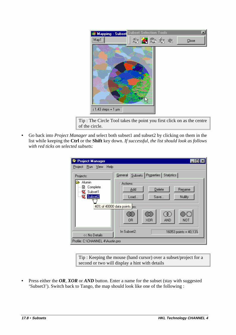
17.8 • Subsets HKL Technology CHANNEL 4
Tip : The Circle Tool takes the point you first click on as the centreof the circle.
• Go back into Project Manager and select both subset1 and subset2 by clicking on them in thelist while keeping the Ctrl or the Shift key down. If successful, the list should look as followswith red ticks on selected subsets:
Tip : Keeping the mouse (hand cursor) over a subset/project for asecond or two will display a hint with details
• Press either the OR, XOR or AND button. Enter a name for the subset (stay with suggested‘Subset3’). Switch back to Tango, the map should look like one of the following :
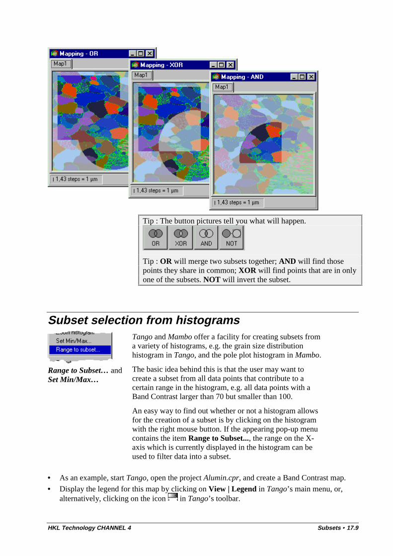
HKL Technology CHANNEL 4 Subsets • 17.9
Tip : The button pictures tell you what will happen.
Tip : OR will merge two subsets together; AND will find thosepoints they share in common; XOR will find points that are in onlyone of the subsets. NOT will invert the subset.
Subset selection from histograms
Range to Subset… andSet Min/Max…
Tango and Mambo offer a facility for creating subsets froma variety of histograms, e.g. the grain size distributionhistogram in Tango, and the pole plot histogram in Mambo.
The basic idea behind this is that the user may want tocreate a subset from all data points that contribute to acertain range in the histogram, e.g. all data points with aBand Contrast larger than 70 but smaller than 100.
An easy way to find out whether or not a histogram allowsfor the creation of a subset is by clicking on the histogramwith the right mouse button. If the appearing pop-up menucontains the item Range to Subset..., the range on the X-axis which is currently displayed in the histogram can beused to filter data into a subset.
• As an example, start Tango, open the project Alumin.cpr, and create a Band Contrast map.
• Display the legend for this map by clicking on View | Legend in Tango’s main menu, or,alternatively, clicking on the icon in Tango’s toolbar.
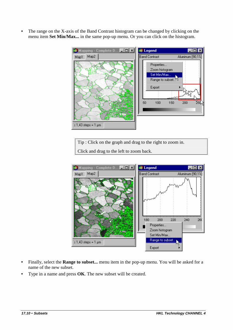
17.10 • Subsets HKL Technology CHANNEL 4
• The range on the X-axis of the Band Contrast histogram can be changed by clicking on themenu item Set Min/Max... in the same pop-up menu. Or you can click on the histogram.
Tip : Click on the graph and drag to the right to zoom in.
Click and drag to the left to zoom back.
• Finally, select the Range to subset... menu item in the pop-up menu. You will be asked for aname of the new subset.
• Type in a name and press OK. The new subset will be created.
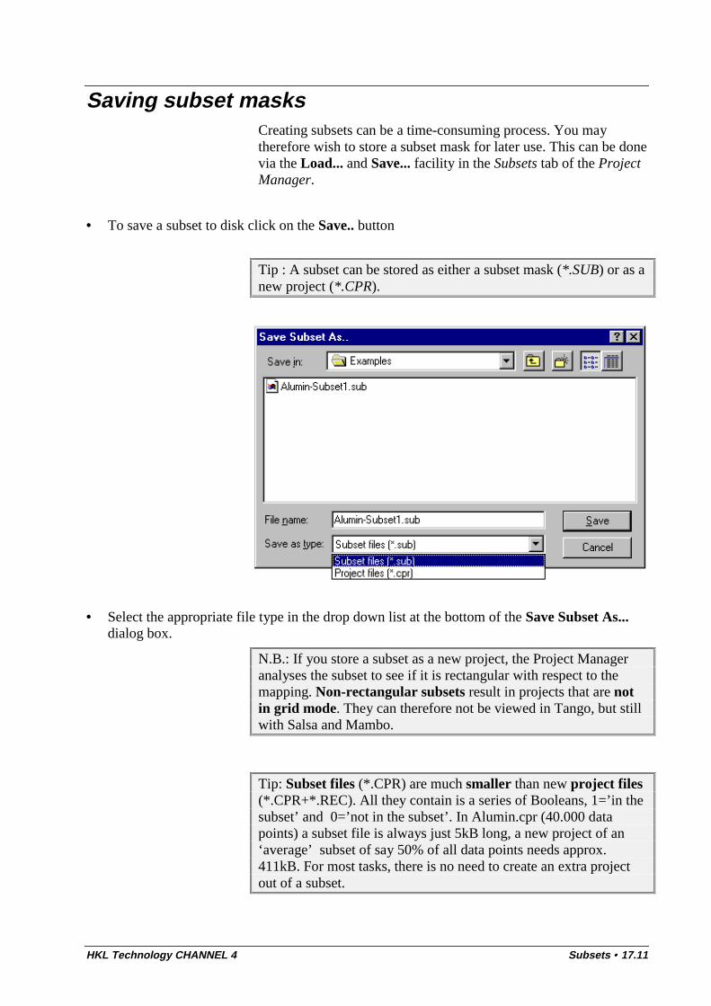
HKL Technology CHANNEL 4 Subsets • 17.11
Saving subset masksCreating subsets can be a time-consuming process. You maytherefore wish to store a subset mask for later use. This can be donevia the Load... and Save... facility in the Subsets tab of the ProjectManager.
• To save a subset to disk click on the Save.. button
Tip : A subset can be stored as either a subset mask (*.SUB) or as anew project (*.CPR).
• Select the appropriate file type in the drop down list at the bottom of the Save Subset As...dialog box.
N.B.: If you store a subset as a new project, the Project Manageranalyses the subset to see if it is rectangular with respect to themapping. Non-rectangular subsets result in projects that are notin grid mode. They can therefore not be viewed in Tango, but stillwith Salsa and Mambo.
Tip: Subset files (*.CPR) are much smaller than new project files(*.CPR+*.REC). All they contain is a series of Booleans, 1=’in thesubset’ and 0=’not in the subset’. In Alumin.cpr (40.000 datapoints) a subset file is always just 5kB long, a new project of an‘average’ subset of say 50% of all data points needs approx.411kB. For most tasks, there is no need to create an extra projectout of a subset.
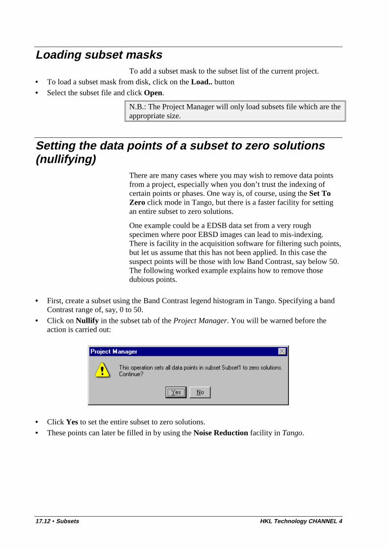
17.12 • Subsets HKL Technology CHANNEL 4
Loading subset masksTo add a subset mask to the subset list of the current project.
• To load a subset mask from disk, click on the Load.. button• Select the subset file and click Open.
N.B.: The Project Manager will only load subsets file which are theappropriate size.
Setting the data points of a subset to zero solutions(nullifying)
There are many cases where you may wish to remove data pointsfrom a project, especially when you don’t trust the indexing ofcertain points or phases. One way is, of course, using the Set ToZero click mode in Tango, but there is a faster facility for settingan entire subset to zero solutions.
One example could be a EDSB data set from a very roughspecimen where poor EBSD images can lead to mis-indexing.There is facility in the acquisition software for filtering such points,but let us assume that this has not been applied. In this case thesuspect points will be those with low Band Contrast, say below 50.The following worked example explains how to remove thosedubious points.
• First, create a subset using the Band Contrast legend histogram in Tango. Specifying a bandContrast range of, say, 0 to 50.
• Click on Nullify in the subset tab of the Project Manager. You will be warned before theaction is carried out:
• Click Yes to set the entire subset to zero solutions.• These points can later be filled in by using the Noise Reduction facility in Tango.
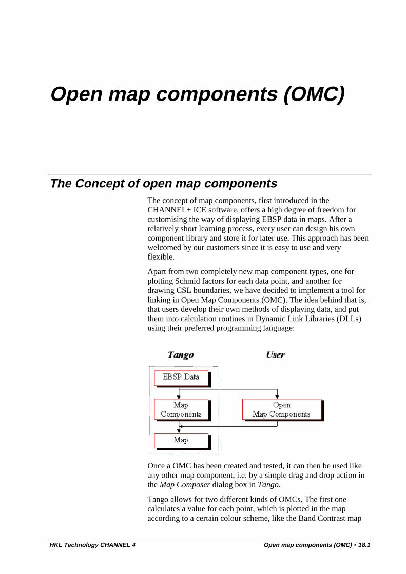
HKL Technology CHANNEL 4 Open map components (OMC) • 18.1
Open map components (OMC)
The Concept of open map componentsThe concept of map components, first introduced in theCHANNEL+ ICE software, offers a high degree of freedom forcustomising the way of displaying EBSP data in maps. After arelatively short learning process, every user can design his owncomponent library and store it for later use. This approach has beenwelcomed by our customers since it is easy to use and veryflexible.
Apart from two completely new map component types, one forplotting Schmid factors for each data point, and another fordrawing CSL boundaries, we have decided to implement a tool forlinking in Open Map Components (OMC). The idea behind that is,that users develop their own methods of displaying data, and putthem into calculation routines in Dynamic Link Libraries (DLLs)using their preferred programming language:
Once a OMC has been created and tested, it can then be used likeany other map component, i.e. by a simple drag and drop action inthe Map Composer dialog box in Tango.
Tango allows for two different kinds of OMCs. The first onecalculates a value for each point, which is plotted in the mapaccording to a certain colour scheme, like the Band Contrast map

18.2 • Open map components (OMC) HKL Technology CHANNEL 4
component (Value-OMC). The second one calculates a colourvalue for each point, which is directly plotted in the map (Colour-OMC).
TaylorCubicX.dll as an example of an OMCYour default component library already contains the mapcomponent TaylorCubicX.dll which is making use of thistechnology. Two other OMCs, TaylorCubicY.dll andTaylorCubicZ.dll ship together with CHANNEL4, and can be foundin the directory where the package has been installed.
We would like to thankDr. Wolfgang Tirschlerand Dr. Cesar Buquefrom TU Dresden,Institut für PhysikalischeMetallkunde,Helmholtzstrasse 7, D-01062, Dresden,Germany, for the fruitfulcollaboration, and Prof.Werner Skrotzky forhelping to make thisproject come true.
The DLLs calculate Taylor factor maps for cubic samplesymmetry and for uniaxial load parallel to the X (Y,Z) direction oryour acquisition surface. These DLLs have been developed in ajoint project between HKL Technology and TU Dresden, Germany.
Explore the property dialog box of this map component byselecting Components | Component Manager.... Mark the mapcomponent Taylor Cubic || X component and click on the buttonProperties (or just double click the map component in the list).
You can now look through the tabs and see what the defaultsettings are.
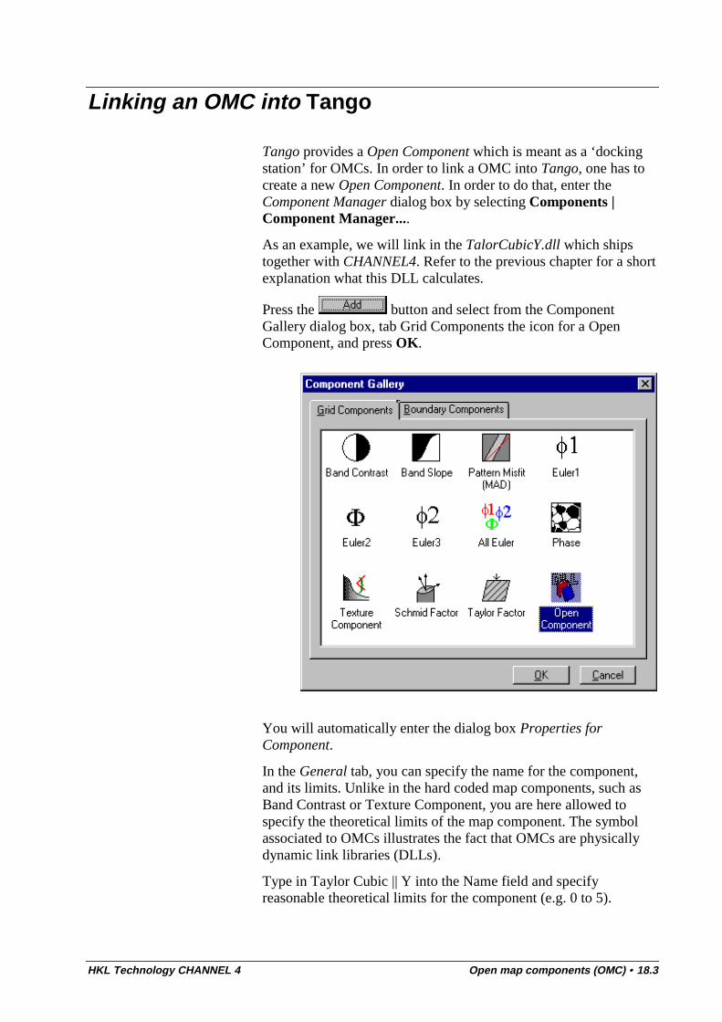
HKL Technology CHANNEL 4 Open map components (OMC) • 18.3
Linking an OMC into Tango
Tango provides a Open Component which is meant as a ‘dockingstation’ for OMCs. In order to link a OMC into Tango, one has tocreate a new Open Component. In order to do that, enter theComponent Manager dialog box by selecting Components |Component Manager....
As an example, we will link in the TalorCubicY.dll which shipstogether with CHANNEL4. Refer to the previous chapter for a shortexplanation what this DLL calculates.
Press the button and select from the ComponentGallery dialog box, tab Grid Components the icon for a OpenComponent, and press OK.
You will automatically enter the dialog box Properties forComponent.
In the General tab, you can specify the name for the component,and its limits. Unlike in the hard coded map components, such asBand Contrast or Texture Component, you are here allowed tospecify the theoretical limits of the map component. The symbolassociated to OMCs illustrates the fact that OMCs are physicallydynamic link libraries (DLLs).
Type in Taylor Cubic || Y into the Name field and specifyreasonable theoretical limits for the component (e.g. 0 to 5).
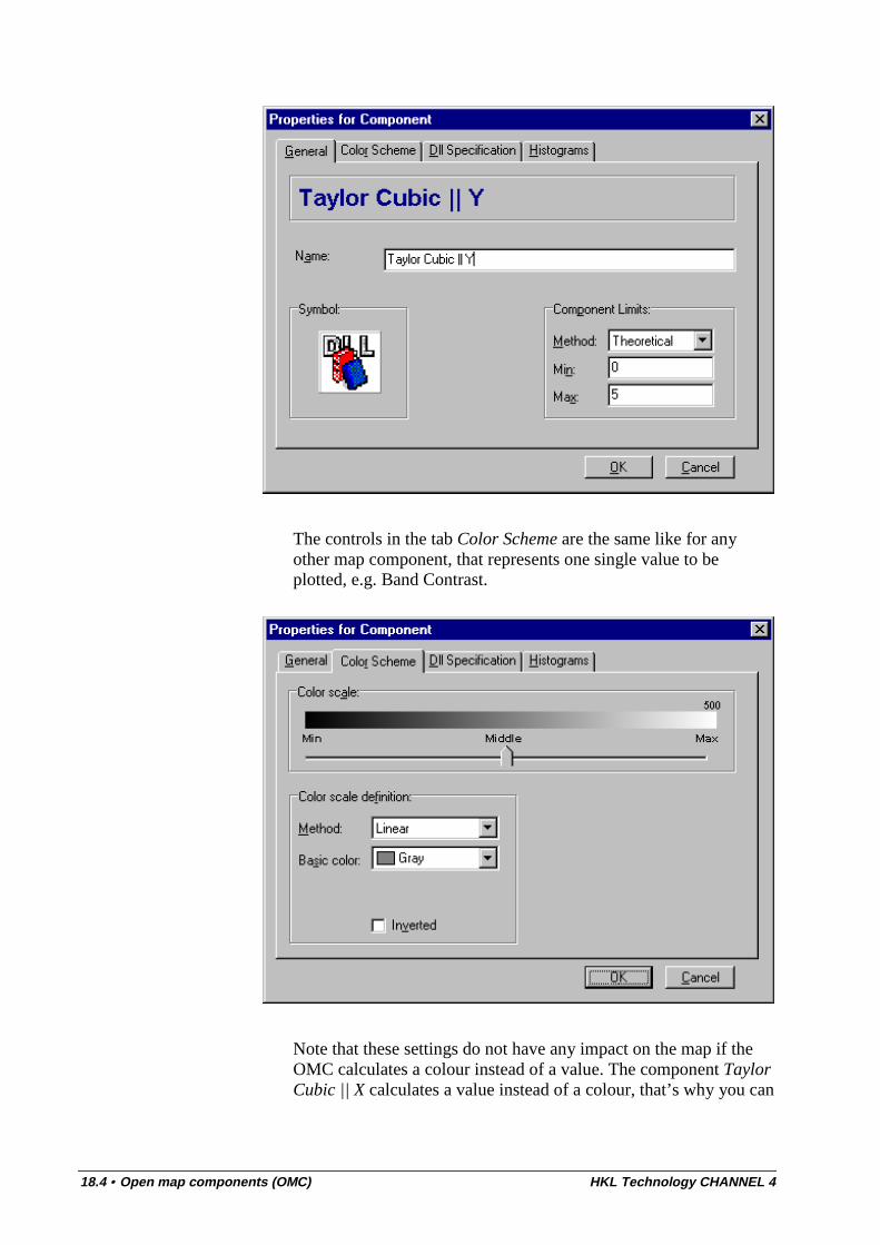
18.4 • Open map components (OMC) HKL Technology CHANNEL 4
The controls in the tab Color Scheme are the same like for anyother map component, that represents one single value to beplotted, e.g. Band Contrast.
Note that these settings do not have any impact on the map if theOMC calculates a colour instead of a value. The component TaylorCubic || X calculates a value instead of a colour, that’s why you can
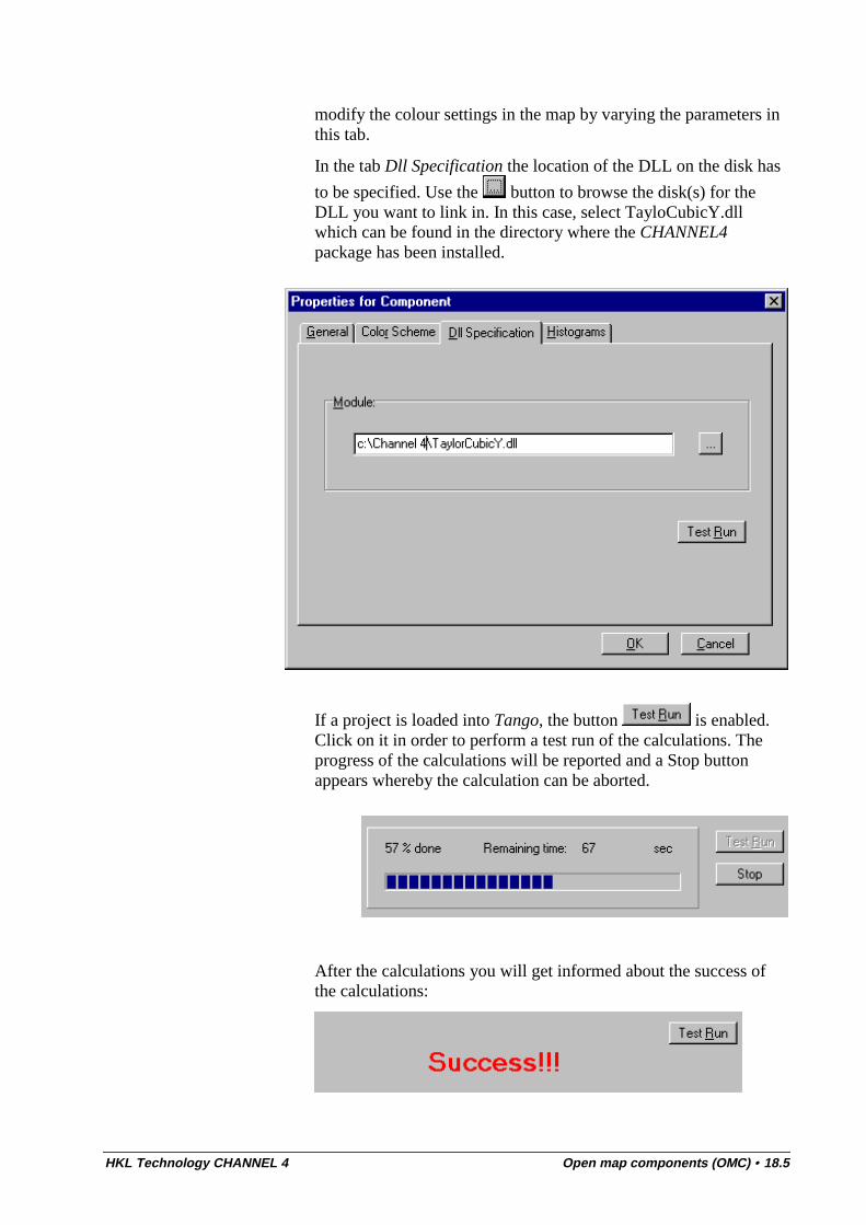
HKL Technology CHANNEL 4 Open map components (OMC) • 18.5
modify the colour settings in the map by varying the parameters inthis tab.
In the tab Dll Specification the location of the DLL on the disk has
to be specified. Use the button to browse the disk(s) for theDLL you want to link in. In this case, select TayloCubicY.dllwhich can be found in the directory where the CHANNEL4package has been installed.
If a project is loaded into Tango, the button is enabled.Click on it in order to perform a test run of the calculations. Theprogress of the calculations will be reported and a Stop buttonappears whereby the calculation can be aborted.
After the calculations you will get informed about the success ofthe calculations:
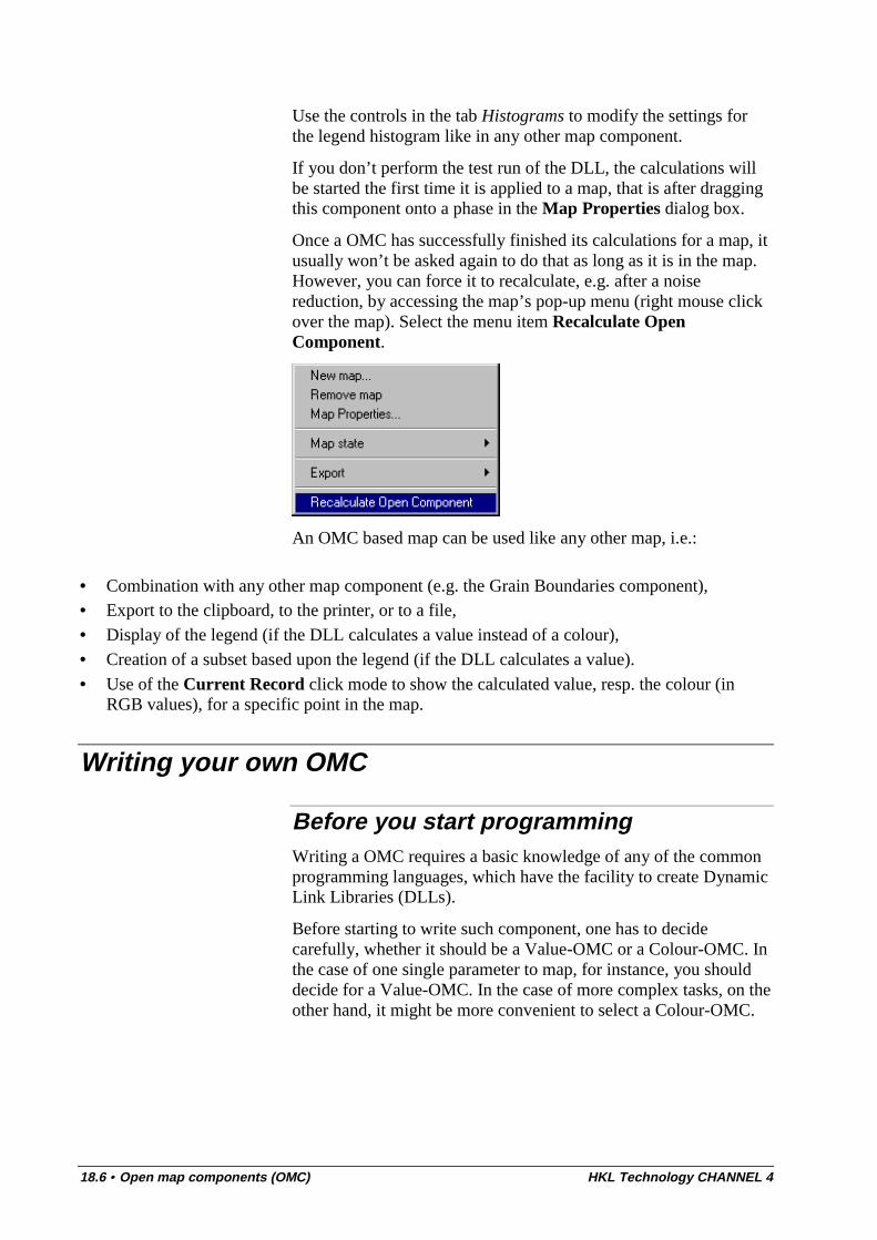
18.6 • Open map components (OMC) HKL Technology CHANNEL 4
Use the controls in the tab Histograms to modify the settings forthe legend histogram like in any other map component.
If you don’t perform the test run of the DLL, the calculations willbe started the first time it is applied to a map, that is after draggingthis component onto a phase in the Map Properties dialog box.
Once a OMC has successfully finished its calculations for a map, itusually won’t be asked again to do that as long as it is in the map.However, you can force it to recalculate, e.g. after a noisereduction, by accessing the map’s pop-up menu (right mouse clickover the map). Select the menu item Recalculate OpenComponent.
An OMC based map can be used like any other map, i.e.:
• Combination with any other map component (e.g. the Grain Boundaries component),• Export to the clipboard, to the printer, or to a file,• Display of the legend (if the DLL calculates a value instead of a colour),• Creation of a subset based upon the legend (if the DLL calculates a value).
• Use of the Current Record click mode to show the calculated value, resp. the colour (inRGB values), for a specific point in the map.
Writing your own OMC
Before you start programmingWriting a OMC requires a basic knowledge of any of the commonprogramming languages, which have the facility to create DynamicLink Libraries (DLLs).
Before starting to write such component, one has to decidecarefully, whether it should be a Value-OMC or a Colour-OMC. Inthe case of one single parameter to map, for instance, you shoulddecide for a Value-OMC. In the case of more complex tasks, on theother hand, it might be more convenient to select a Colour-OMC.
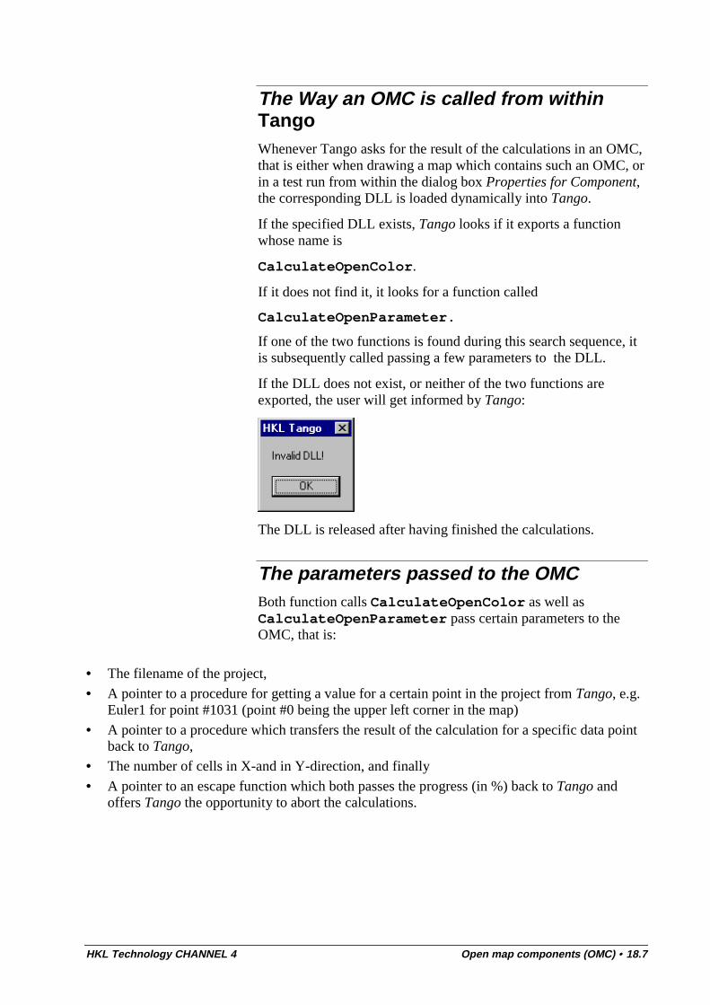
HKL Technology CHANNEL 4 Open map components (OMC) • 18.7
The Way an OMC is called from withinTangoWhenever Tango asks for the result of the calculations in an OMC,that is either when drawing a map which contains such an OMC, orin a test run from within the dialog box Properties for Component,the corresponding DLL is loaded dynamically into Tango.
If the specified DLL exists, Tango looks if it exports a functionwhose name is
CalculateOpenColor.
If it does not find it, it looks for a function called
CalculateOpenParameter.
If one of the two functions is found during this search sequence, itis subsequently called passing a few parameters to the DLL.
If the DLL does not exist, or neither of the two functions areexported, the user will get informed by Tango:
The DLL is released after having finished the calculations.
The parameters passed to the OMCBoth function calls CalculateOpenColor as well asCalculateOpenParameter pass certain parameters to theOMC, that is:
• The filename of the project,
• A pointer to a procedure for getting a value for a certain point in the project from Tango, e.g.Euler1 for point #1031 (point #0 being the upper left corner in the map)
• A pointer to a procedure which transfers the result of the calculation for a specific data pointback to Tango,
• The number of cells in X-and in Y-direction, and finally
• A pointer to an escape function which both passes the progress (in %) back to Tango andoffers Tango the opportunity to abort the calculations.

18.8 • Open map components (OMC) HKL Technology CHANNEL 4
Example OMCs written in Borland
DelphiThe easiest way of understanding how such an OMC can bedesigned, is to have a look at the source code of a working OMC.HKL Technology therefore provides the source code of a fewexamples, for Value-OMCs as well as for Colour-OMCs.
The examples discussed in this section are written in Borland
Delphi (which is based upon TurboPascal). They are calledUserCompValue.dpr and UserCompColor.dpr, respectively, andcan be found in the subdirectory \OMCExamples\DelphiOMC,starting from the directory where the package has been installed.
The first OMC converts the first Euler angle of a measurementfrom radians into degree, and the second OMC takes the BandContrast of each point and converts it into a grey value (like thestandard Band Contrast map component when it uses its defaultsettings).
The code of UserCompValue.dpr is shown in the following listing:
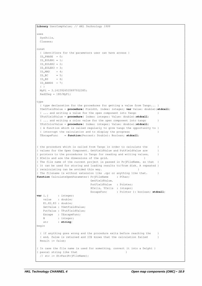
HKL Technology CHANNEL 4 Open map components (OMC) • 18.9
Library UserCompValue; // HKL Technology 1999
uses
SysUtils,
Classes;
const
{ identifiers for the parameters user can have access }
ID_PHASE = 0;
ID_EULER1 = 1;
ID_EULER2 = 2;
ID_EULER3 = 3;
ID_MAD = 4;
ID_BC = 5;
ID_BS = 6;
ID_BANDS = 7;
{ }
MyPi = 3.1415926535897932385;
Rad2Deg = 180/MyPi;
type
{ type declaration for the procedures for getting a value from Tango... }
TGetFieldValue = procedure( FieldID, Index: integer; var Value: double);stdcall;
{ ... and writing a value for the open component into Tango }
TPutFieldValue = procedure( Index: integer; Value: double);stdcall;
{ ... and writing a color value for the open component into tango }
TPutColorValue = procedure( Index: integer; Value: double);stdcall;
{ A function which is called regularly to give tango the opportunity to }
{ interrupt the calculation and to display the progress }
TEscapeFunc = function(Percent: Double): Boolean; stdcall;
{ the procedure which is called from Tango in order to calculate the }
{ values for the Open Component. GetFieldValue and PutFieldValue are }
{ pointers to the procedures in Tango for reading and writing values, }
{ XCells and are the dimensions of the grid. }
{ The file name of the current project is passed in PrjFileName, so that }
{ it can be used for storing and loading results to/from disk. A repeated }
{ recalculating can be avoided this way. }
{ The filename is without extension like .cpr or anything like that. }
function CalculateOpenParameter( PrjFileName : PChar;
GetFieldValue,
PutFieldValue : Pointer;
XCells, YCells : integer;
EscapeFunc : Pointer ): boolean; stdcall;
var i,j : integer;
value : double;
E1,E2,E3 : double;
GetValue : TGetFieldValue;
PutValue : TPutFieldValue;
Escape : TEscapeFunc;
N : integer;
str : string;
begin
{ if anything goes wrong and the procedure exits before reaching the }
{ end, false is returned and ICE knows that the calculation failed }
Result := false;
{ In case the file name is used for something, convert it into a Delphi }
{ pascal string like that }
// str := StrPas(PrjFileName);
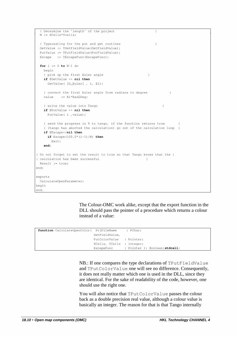
18.10 • Open map components (OMC) HKL Technology CHANNEL 4
{ Determine the ’length’ of the project } N := XCells*Ycells;
{ Typecasting for the put and get routines }
GetValue := TGetFieldValue(GetFieldValue);
PutValue := TPutFieldValue(PutFieldValue);
Escape := TEscapeFunc(EscapeFunc);
for i := 0 to N-1 do
begin
{ pick up the first Euler angle }
if @GetValue <> nil then
GetValue( ID_Euler1 , i, E1);
{ convert the first Euler angle from radians to degree }
value := E1*Rad2Deg;
{ write the value into Tango }
if @PutValue <> nil then
PutValue( i ,value);
{ send the progress in % to tango, if the function returns true }
{ (tango has aborted the calculation) go out of the calculation loop }
if @Escape<>nil then
if Escape(100.0*(i-1)/N) then
Exit;
end;
{ Do not forget to set the result to true so that Tango knows that the }
{ calculation has been successful }
Result := true;
end;
exports
CalculateOpenParameter;
begin
end.
The Colour-OMC work alike, except that the export function in theDLL should pass the pointer of a procedure which returns a colourinstead of a value:
function CalculateOpenColor( PrjFileName : PChar;
GetFieldValue,
PutColorValue : Pointer;
XCells, YCells : integer;
EscapeFunc : Pointer ): Boolean;stdcall;
NB.: If one compares the type declarations of TPutFieldValueand TPutColorValue one will see no difference. Consequently,it does not really matter which one is used in the DLL, since theyare identical. For the sake of readability of the code, however, oneshould use the right one.
You will also notice that TPutColorValue passes the colourback as a double precision real value, although a colour value isbasically an integer. The reason for that is that Tango internally
HKL Technology CHANNEL 4 Open map components (OMC) • 18.11
uses the same array for both a value (real) and a colour. If youdesign your DLL, you don’t have to worry about that. The onlyconsequence is that you can theoretically pass a colour value,which is more precise than integer, which has no effect on thecolours displayed on the screen.
Example OMCs written in Borland C++BuilderIn order to assist C++ software developers, HKL Technology hasalso provided examples in this language. We have selectedBorland C++ Builder for test purposes. However, the codeshould work with other C++ compilers with minor modifications.
The project files are called UserCompValue.bpr andUserCompColor.bpr, respectively, and the C++ files are calledUserCompValue.cpp and UserCompColor.cpp. They can be foundin the subdirectory \OMCExamples\BorlandC++OMC, startingfrom the directory where the package has been installed.
Like in the previous section, the first OMC converts the first Eulerangle of a measurement from radians into degree, and the secondOMC takes the Band Contrast of each point and converts it into agrey value.
The major difference to the Delphi example is that the typedeclaration for the functions GetFieldValue,PutFieldValue, and EscapeFunc are done right within theparameter list of the functions.
Note that passing a value to a function by reference can be done inC++ by the &-symbol which corresponds to the var syntax inTurboPascal. This is a requirement for the 3rd parameter in thefunction GetFieldValue function and must not be forgotten!
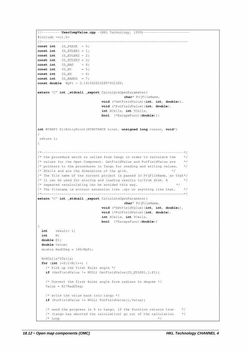
18.12 • Open map components (OMC) HKL Technology CHANNEL 4
//--------- UserCompValue.cpp -(HKL Technology, 1999)-----------------------
#include <vcl.h>
//-------------------------------------------------------------------------
const int ID_PHASE = 0;
const int ID_EULER1 = 1;
const int ID_EULER2 = 2;
const int ID_EULER3 = 3;
const int ID_MAD = 4;
const int ID_BC = 5;
const int ID_BS = 6;
const int ID_BANDS = 7;
const double MyPi = 3.1415926535897932385;
extern "C" int _stdcall _export CalculateOpenParameter(
char* PrjFileName,
void (*GetFieldValue)(int, int, double&),
void (*PutFieldValue)(int, double),
int XCells, int YCells,
bool (*EscapeFunc)(double));
int WINAPI DllEntryPoint(HINSTANCE hinst, unsigned long reason, void*)
{
return 1;
}
/*-----------------------------------------------------------------------*/
/* the procedure which is called from Tango in order to calculate the */
/* values for the Open Component. GetFieldValue and PutFieldValue are */
/* pointers to the procedures in Tango for reading and writing values, */
/* XCells and are the dimensions of the grid. */
/* The file name of the current project is passed in PrjFileName, so that*/
/* it can be used for storing and loading results to/from disk. A */
/* repeated recalculating can be avoided this way. */
/* The filename is without extension like .cpr or anything like that. */
/*-----------------------------------------------------------------------*/
extern "C" int _stdcall _export CalculateOpenParameter(
char* PrjFileName,
void (*GetFieldValue)(int, int, double&),
void (*PutFieldValue)(int, double),
int XCells, int YCells,
bool (*EscapeFunc)(double))
{
int result= 1;
int N;
double E1;
double Value;
double Rad2Deg = 180/MyPi;
N=XCells*YCells;
for (int i=0;i<N;i++) {
/* Pick up the first Euler angle */
if (GetFieldValue != NULL) GetFieldValue(ID_EULER1,i,E1);
/* Convert the first Euler angle from radians to degree */
Value = E1*Rad2Deg;
/* write the value back into tango */
if (PutFieldValue != NULL) PutFieldValue(i,Value);
/* send the progress in % to tango, if the function returns true */
/* (tango has aborted the calculation) go out of the calculation */
/* loop */

HKL Technology CHANNEL 4 Open map components (OMC) • 18.13
if (EscapeFunc != NULL) if (EscapeFunc(100.0*(i-1)/N)) {
result = 0;
break;
}
}
/* Do not forget to set the result so that Tango knows whether or not */
/* the calculation has been successful */
return result;
}

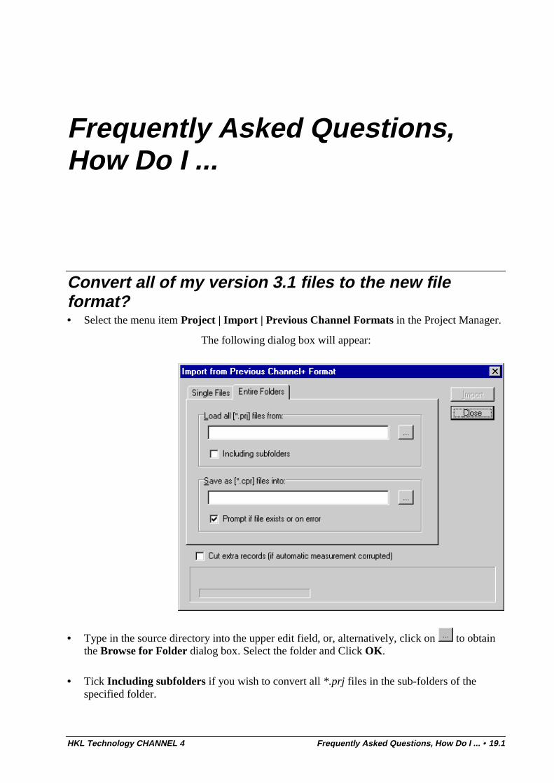
HKL Technology CHANNEL 4 Frequently Asked Questions, How Do I ... • 19.1
Frequently Asked Questions,How Do I ...
Convert all of my version 3.1 files to the new fileformat?• Select the menu item Project | Import | Previous Channel Formats in the Project Manager.
The following dialog box will appear:
• Type in the source directory into the upper edit field, or, alternatively, click on to obtainthe Browse for Folder dialog box. Select the folder and Click OK.
• Tick Including subfolders if you wish to convert all *.prj files in the sub-folders of thespecified folder.
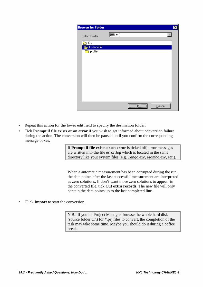
19.2 • Frequently Asked Questions, How Do I ... HKL Technology CHANNEL 4
• Repeat this action for the lower edit field to specify the destination folder.
• Tick Prompt if file exists or on error if you wish to get informed about conversion failureduring the action. The conversion will then be paused until you confirm the correspondingmessage boxes.
If Prompt if file exists or on error is ticked off, error messagesare written into the file error.log which is located in the samedirectory like your system files (e.g. Tango.exe, Mambo.exe, etc.).
When a automatic measurement has been corrupted during the run,the data points after the last successful measurement are interpretedas zero solutions. If don’t want those zero solutions to appear inthe converted file, tick Cut extra records. The new file will onlycontain the data points up to the last completed line.
• Click Import to start the conversion.
N.B.: If you let Project Manager browse the whole hard disk(source folder C:\) for *.prj files to convert, the completion of thetask may take some time. Maybe you should do it during a coffeebreak.
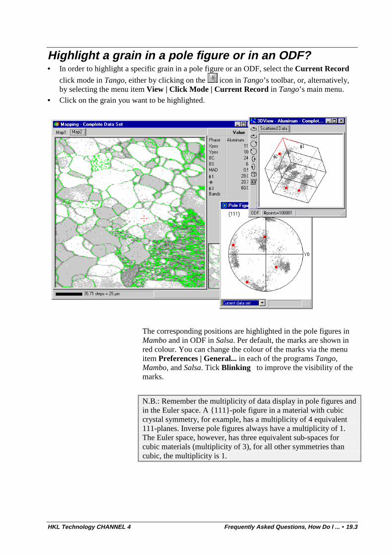
HKL Technology CHANNEL 4 Frequently Asked Questions, How Do I ... • 19.3
Highlight a grain in a pole figure or in an ODF?• In order to highlight a specific grain in a pole figure or an ODF, select the Current Record
click mode in Tango, either by clicking on the icon in Tango’s toolbar, or, alternatively,by selecting the menu item View | Click Mode | Current Record in Tango’s main menu.
• Click on the grain you want to be highlighted.
The corresponding positions are highlighted in the pole figures inMambo and in ODF in Salsa. Per default, the marks are shown inred colour. You can change the colour of the marks via the menuitem Preferences | General... in each of the programs Tango,Mambo, and Salsa. Tick Blinking to improve the visibility of themarks.
N.B.: Remember the multiplicity of data display in pole figures andin the Euler space. A {111}-pole figure in a material with cubiccrystal symmetry, for example, has a multiplicity of 4 equivalent111-planes. Inverse pole figures always have a multiplicity of 1.The Euler space, however, has three equivalent sub-spaces forcubic materials (multiplicity of 3), for all other symmetries thancubic, the multiplicity is 1.
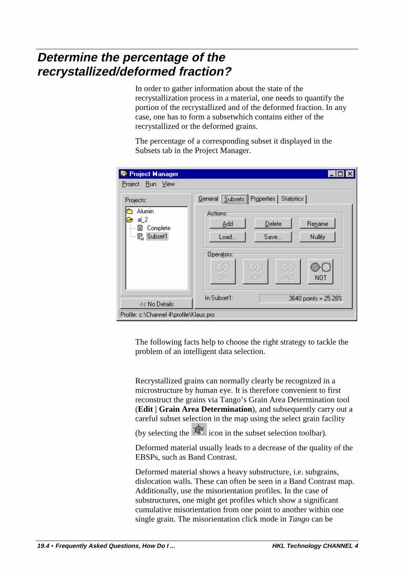
19.4 • Frequently Asked Questions, How Do I ... HKL Technology CHANNEL 4
Determine the percentage of therecrystallized/deformed fraction?
In order to gather information about the state of therecrystallization process in a material, one needs to quantify theportion of the recrystallized and of the deformed fraction. In anycase, one has to form a subsetwhich contains either of therecrystallized or the deformed grains.
The percentage of a corresponding subset it displayed in theSubsets tab in the Project Manager.
The following facts help to choose the right strategy to tackle theproblem of an intelligent data selection.
Recrystallized grains can normally clearly be recognized in amicrostructure by human eye. It is therefore convenient to firstreconstruct the grains via Tango’s Grain Area Determination tool(Edit | Grain Area Determination), and subsequently carry out acareful subset selection in the map using the select grain facility
(by selecting the icon in the subset selection toolbar).
Deformed material usually leads to a decrease of the quality of theEBSPs, such as Band Contrast.
Deformed material shows a heavy substructure, i.e. subgrains,dislocation walls. These can often be seen in a Band Contrast map.Additionally, use the misorientation profiles. In the case ofsubstructures, one might get profiles which show a significantcumulative misorientation from one point to another within onesingle grain. The misorientation click mode in Tango can be
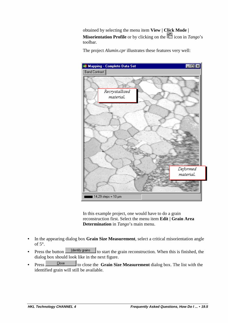
HKL Technology CHANNEL 4 Frequently Asked Questions, How Do I ... • 19.5
obtained by selecting the menu item View | Click Mode |
Misorientation Profile or by clicking on the icon in Tango’stoolbar.
The project Alumin.cpr illustrates these features very well:
In this example project, one would have to do a grainreconstruction first. Select the menu item Edit | Grain AreaDetermination in Tango’s main menu.
• In the appearing dialog box Grain Size Measurement, select a critical misorientation angleof 5°.
• Press the button to start the grain reconstruction. When this is finished, thedialog box should look like in the next figure.
• Press to close the Grain Size Measurement dialog box. The list with theidentified grain will still be available.
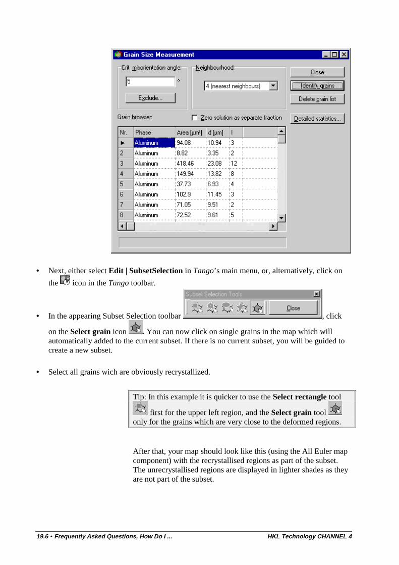
19.6 • Frequently Asked Questions, How Do I ... HKL Technology CHANNEL 4
• Next, either select Edit | SubsetSelection in Tango’s main menu, or, alternatively, click on
the icon in the Tango toolbar.
• In the appearing Subset Selection toolbar , click
on the Select grain icon . You can now click on single grains in the map which willautomatically added to the current subset. If there is no current subset, you will be guided tocreate a new subset.
• Select all grains wich are obviously recrystallized.
Tip: In this example it is quicker to use the Select rectangle tool
first for the upper left region, and the Select grain tool only for the grains which are very close to the deformed regions.
After that, your map should look like this (using the All Euler mapcomponent) with the recrystallised regions as part of the subset.The unrecrystallised regions are displayed in lighter shades as theyare not part of the subset.
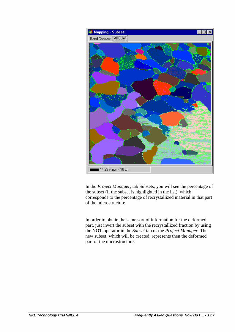
HKL Technology CHANNEL 4 Frequently Asked Questions, How Do I ... • 19.7
In the Project Manager, tab Subsets, you will see the percentage ofthe subset (if the subset is highlighted in the list), whichcorresponds to the percentage of recrystallized material in that partof the microstructure.
In order to obtain the same sort of information for the deformedpart, just invert the subset with the recrystallized fraction by usingthe NOT-operator in the Subset tab of the Project Manager. Thenew subset, which will be created, represents then the deformedpart of the microstructure.
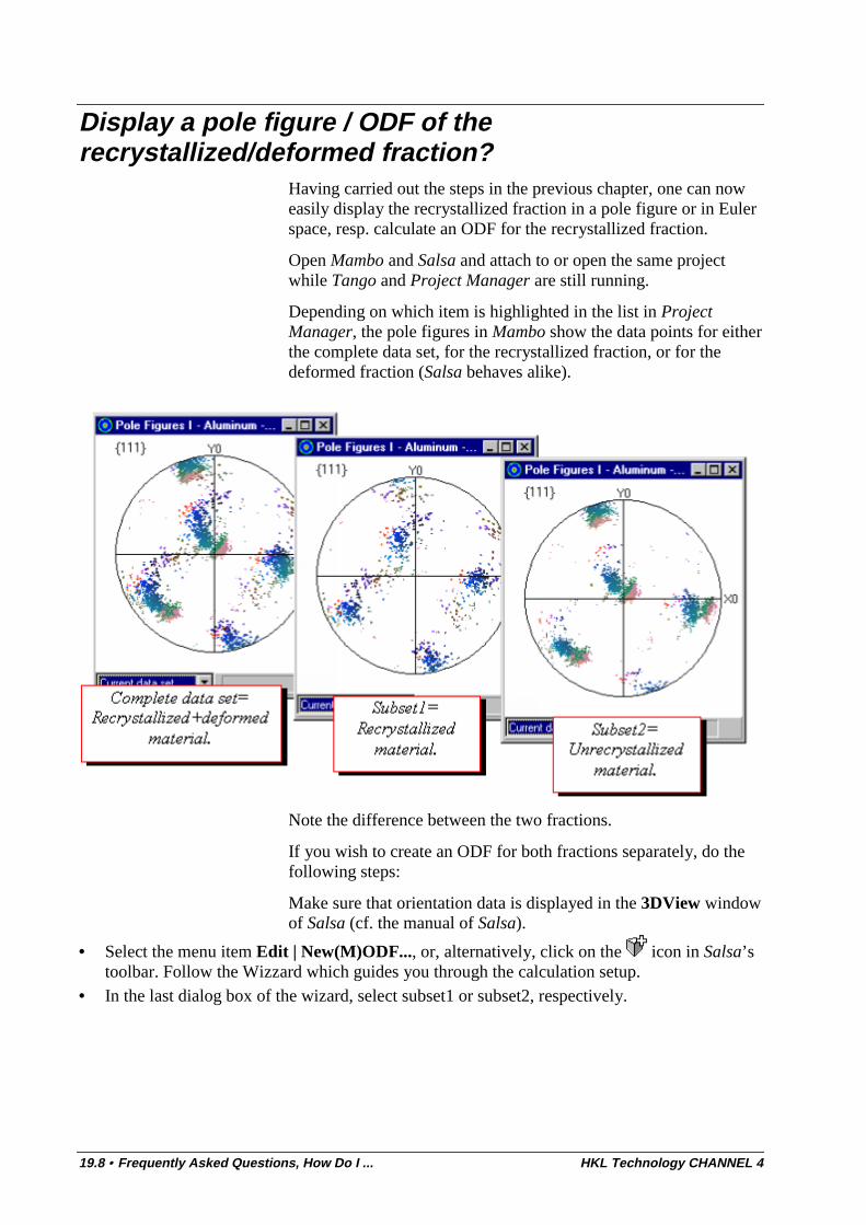
19.8 • Frequently Asked Questions, How Do I ... HKL Technology CHANNEL 4
Display a pole figure / ODF of therecrystallized/deformed fraction?
Having carried out the steps in the previous chapter, one can noweasily display the recrystallized fraction in a pole figure or in Eulerspace, resp. calculate an ODF for the recrystallized fraction.
Open Mambo and Salsa and attach to or open the same projectwhile Tango and Project Manager are still running.
Depending on which item is highlighted in the list in ProjectManager, the pole figures in Mambo show the data points for eitherthe complete data set, for the recrystallized fraction, or for thedeformed fraction (Salsa behaves alike).
Note the difference between the two fractions.
If you wish to create an ODF for both fractions separately, do thefollowing steps:
Make sure that orientation data is displayed in the 3DView windowof Salsa (cf. the manual of Salsa).
• Select the menu item Edit | New(M)ODF..., or, alternatively, click on the icon in Salsa’stoolbar. Follow the Wizzard which guides you through the calculation setup.
• In the last dialog box of the wizard, select subset1 or subset2, respectively.
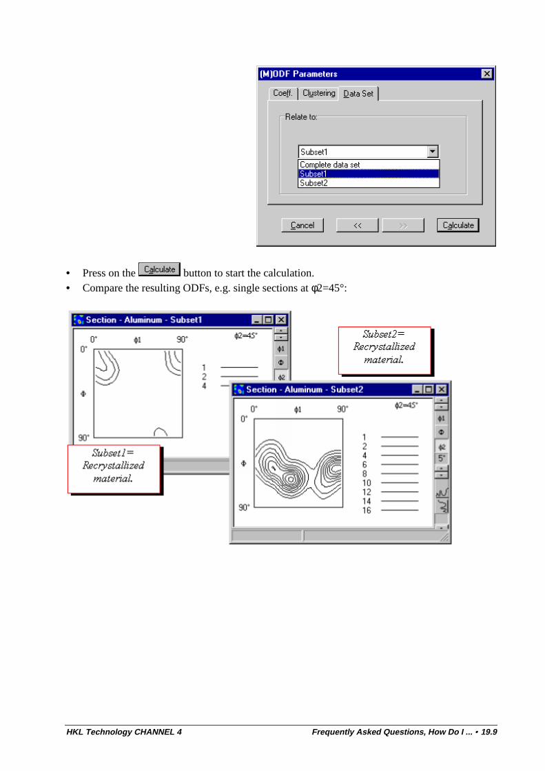
HKL Technology CHANNEL 4 Frequently Asked Questions, How Do I ... • 19.9
• Press on the button to start the calculation.• Compare the resulting ODFs, e.g. single sections at φ2=45°:
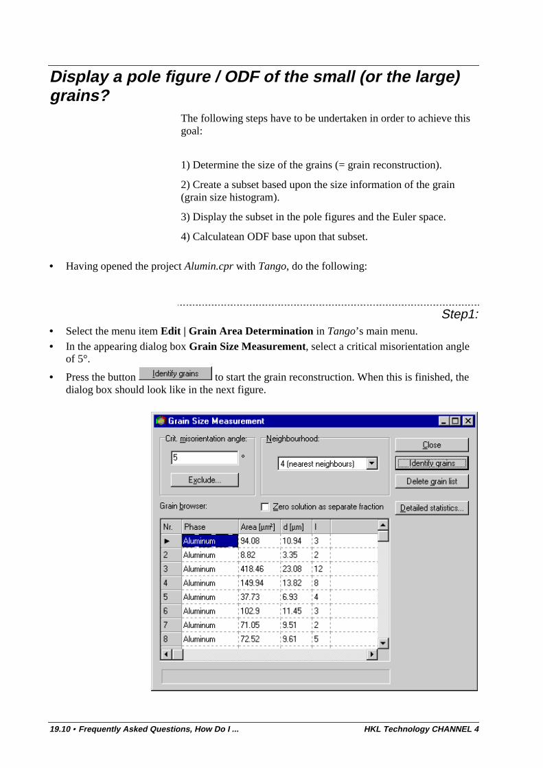
19.10 • Frequently Asked Questions, How Do I ... HKL Technology CHANNEL 4
Display a pole figure / ODF of the small (or the large)grains?
The following steps have to be undertaken in order to achieve thisgoal:
1) Determine the size of the grains (= grain reconstruction).
2) Create a subset based upon the size information of the grain(grain size histogram).
3) Display the subset in the pole figures and the Euler space.
4) Calculatean ODF base upon that subset.
• Having opened the project Alumin.cpr with Tango, do the following:
Step1:• Select the menu item Edit | Grain Area Determination in Tango’s main menu.
• In the appearing dialog box Grain Size Measurement, select a critical misorientation angleof 5°.
• Press the button to start the grain reconstruction. When this is finished, thedialog box should look like in the next figure.
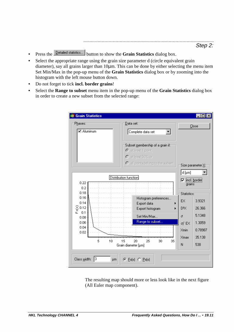
HKL Technology CHANNEL 4 Frequently Asked Questions, How Do I ... • 19.11
Step 2:
• Press the button to show the Grain Statistics dialog box.
• Select the appropriate range using the grain size parameter d (circle equivalent graindiameter), say all grains larger than 10µm. This can be done by either selecting the menu itemSet Min/Max in the pop-up menu of the Grain Statistics dialog box or by zooming into thehistogram with the left mouse button down.
• Do not forget to tick incl. border grains!
• Select the Range to subset menu item in the pop-up menu of the Grain Statistics dialog boxin order to create a new subset from the selected range:
The resulting map should more or less look like in the next figure(All Euler map component).
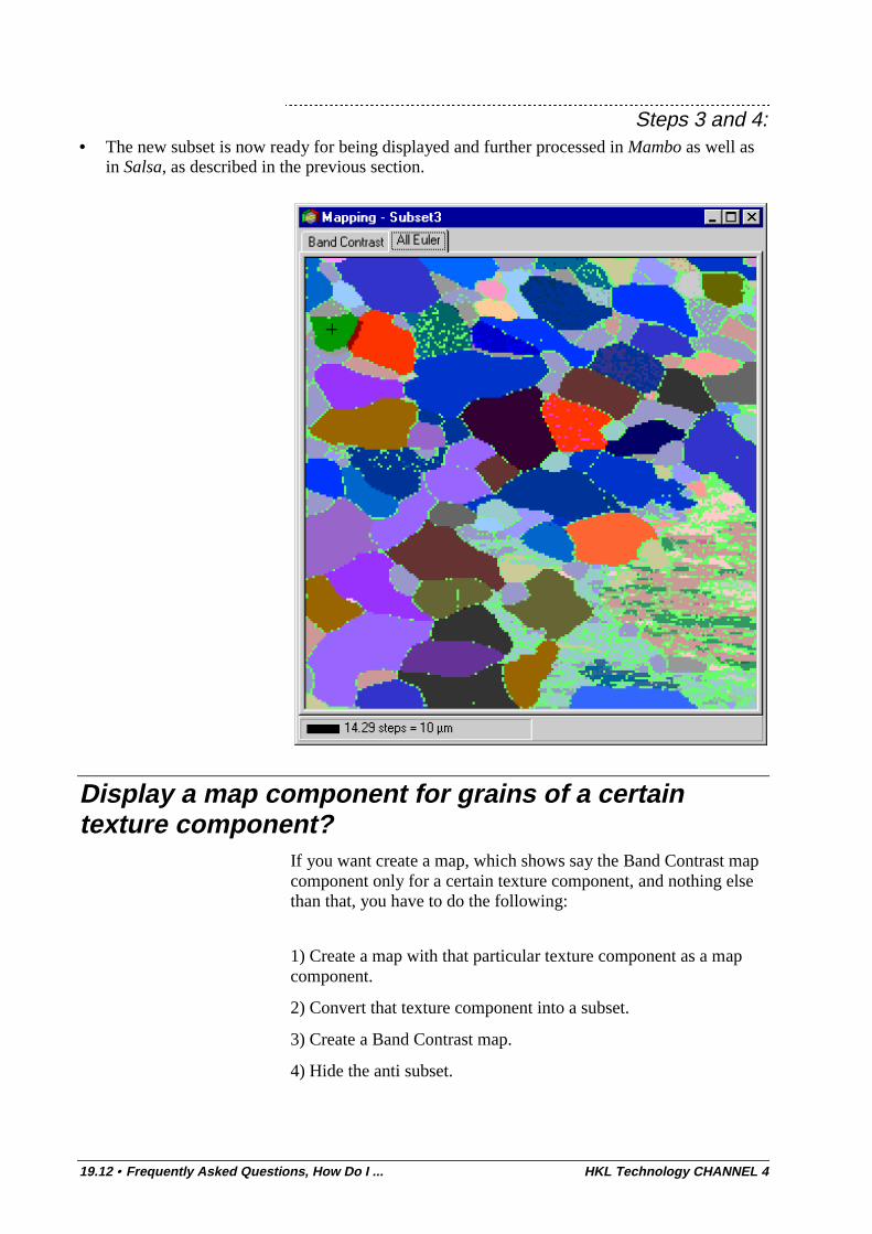
19.12 • Frequently Asked Questions, How Do I ... HKL Technology CHANNEL 4
Steps 3 and 4:• The new subset is now ready for being displayed and further processed in Mambo as well as
in Salsa, as described in the previous section.
Display a map component for grains of a certaintexture component?
If you want create a map, which shows say the Band Contrast mapcomponent only for a certain texture component, and nothing elsethan that, you have to do the following:
1) Create a map with that particular texture component as a mapcomponent.
2) Convert that texture component into a subset.
3) Create a Band Contrast map.
4) Hide the anti subset.
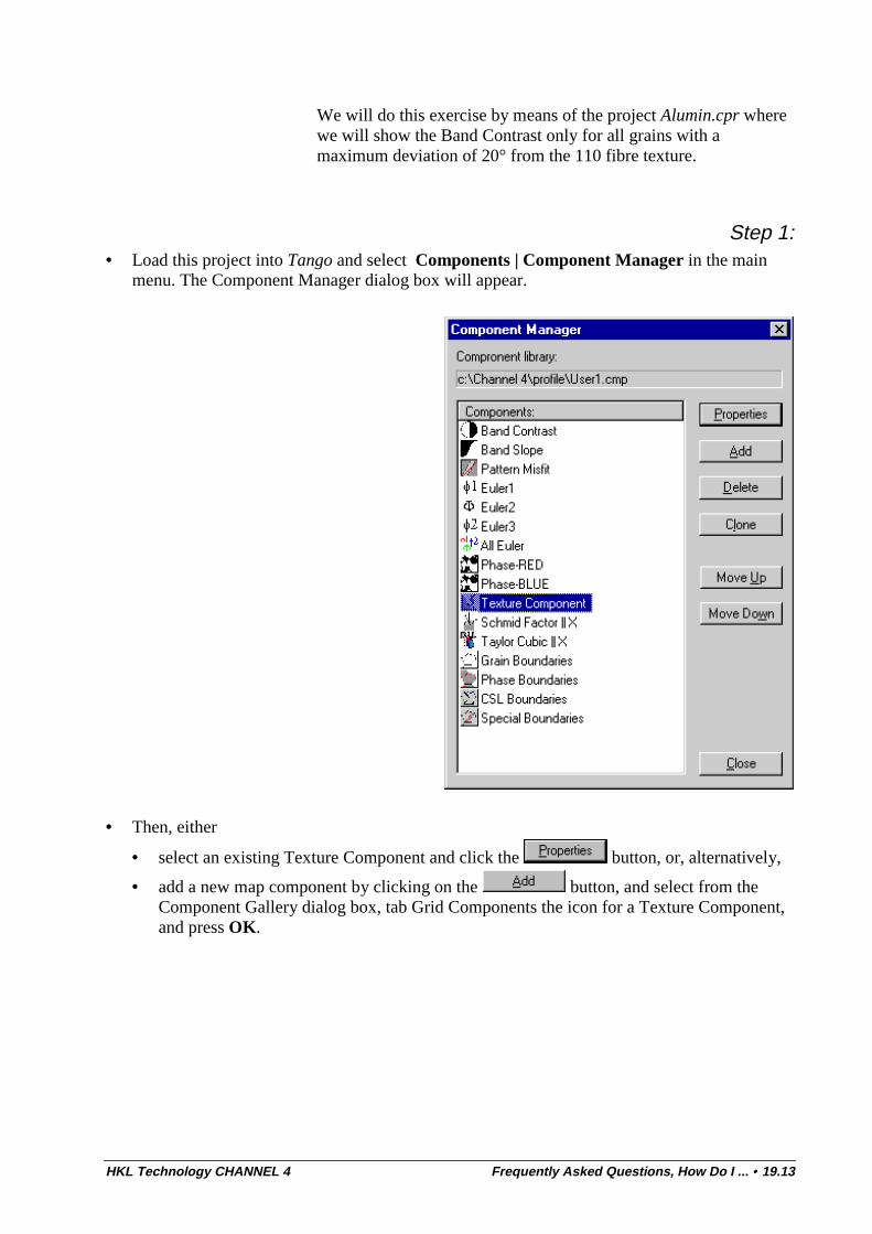
HKL Technology CHANNEL 4 Frequently Asked Questions, How Do I ... • 19.13
We will do this exercise by means of the project Alumin.cpr wherewe will show the Band Contrast only for all grains with amaximum deviation of 20° from the 110 fibre texture.
Step 1:• Load this project into Tango and select Components | Component Manager in the main
menu. The Component Manager dialog box will appear.
• Then, either
• select an existing Texture Component and click the button, or, alternatively,
• add a new map component by clicking on the button, and select from theComponent Gallery dialog box, tab Grid Components the icon for a Texture Component,and press OK.
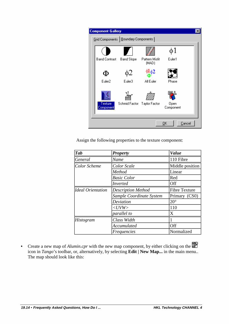
19.14 • Frequently Asked Questions, How Do I ... HKL Technology CHANNEL 4
Assign the following properties to the texture component:
Tab Property ValueGeneral Name 110 Fibre
Color Scheme Color Scale Middle positionMethod LinearBasic Color RedInverted Off
Ideal Orientation Description Method Fibre TextureSample Coordinate System Primary (CS0)Deviation 20°<UVW> 110parallel to X
Histogram Class Width 1Accumulated OffFrequencies Normalized
• Create a new map of Alumin.cpr with the new map component, by either clicking on the icon in Tango’s toolbar, or, alternatively, by selecting Edit | New Map... in the main menu..The map should look like this:
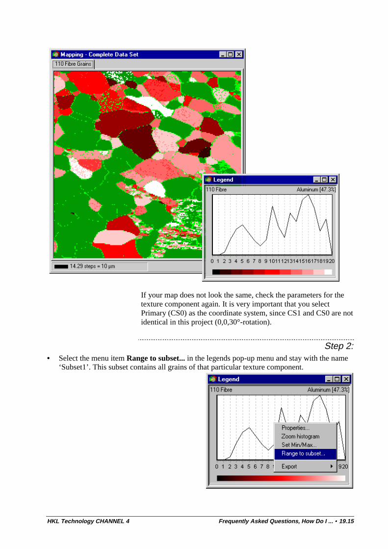
HKL Technology CHANNEL 4 Frequently Asked Questions, How Do I ... • 19.15
If your map does not look the same, check the parameters for thetexture component again. It is very important that you selectPrimary (CS0) as the coordinate system, since CS1 and CS0 are notidentical in this project (0,0,30°-rotation).
Step 2:• Select the menu item Range to subset... in the legends pop-up menu and stay with the name
‘Subset1’. This subset contains all grains of that particular texture component.
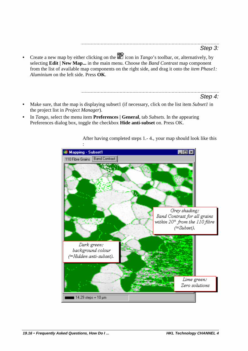
19.16 • Frequently Asked Questions, How Do I ... HKL Technology CHANNEL 4
Step 3:
• Create a new map by either clicking on the icon in Tango’s toolbar, or, alternatively, byselecting Edit | New Map... in the main menu. Choose the Band Contrast map componentfrom the list of available map components on the right side, and drag it onto the item Phase1:Aluminium on the left side. Press OK.
Step 4:• Make sure, that the map is displaying subset1 (if necessary, click on the list item Subset1 in
the project list in Project Manager).
• In Tango, select the menu item Preferences | General, tab Subsets. In the appearingPreferences dialog box, toggle the checkbox Hide anti-subset on. Press OK.
After having completed steps 1.- 4., your map should look like this:
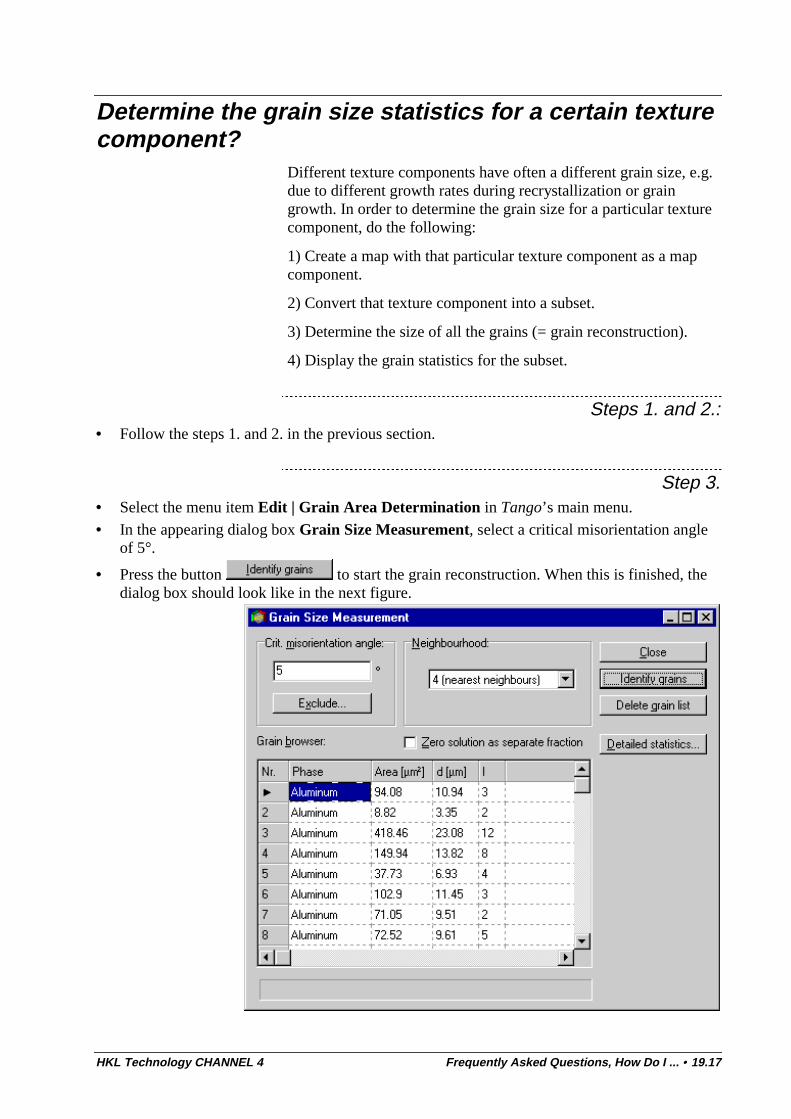
HKL Technology CHANNEL 4 Frequently Asked Questions, How Do I ... • 19.17
Determine the grain size statistics for a certain texturecomponent?
Different texture components have often a different grain size, e.g.due to different growth rates during recrystallization or graingrowth. In order to determine the grain size for a particular texturecomponent, do the following:
1) Create a map with that particular texture component as a mapcomponent.
2) Convert that texture component into a subset.
3) Determine the size of all the grains (= grain reconstruction).
4) Display the grain statistics for the subset.
Steps 1. and 2.:• Follow the steps 1. and 2. in the previous section.
Step 3.• Select the menu item Edit | Grain Area Determination in Tango’s main menu.
• In the appearing dialog box Grain Size Measurement, select a critical misorientation angleof 5°.
• Press the button to start the grain reconstruction. When this is finished, thedialog box should look like in the next figure.
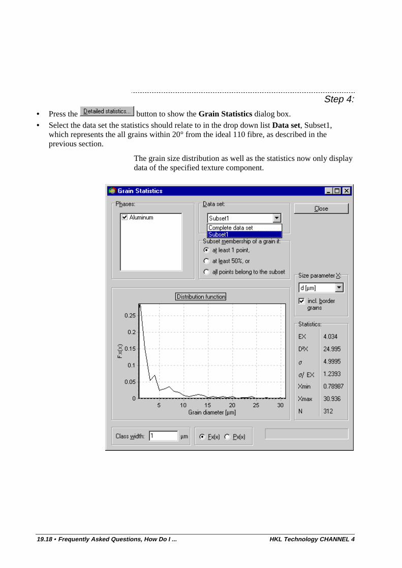
19.18 • Frequently Asked Questions, How Do I ... HKL Technology CHANNEL 4
Step 4:
• Press the button to show the Grain Statistics dialog box.
• Select the data set the statistics should relate to in the drop down list Data set, Subset1,which represents the all grains within 20° from the ideal 110 fibre, as described in theprevious section.
The grain size distribution as well as the statistics now only displaydata of the specified texture component.
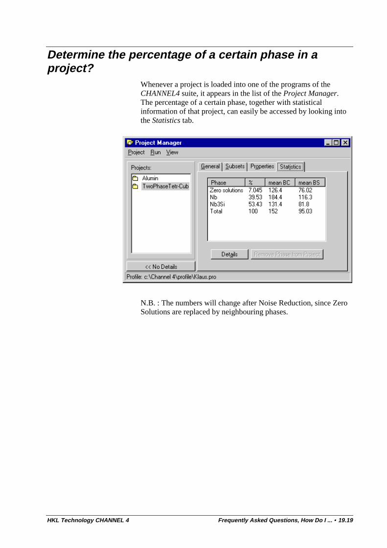
HKL Technology CHANNEL 4 Frequently Asked Questions, How Do I ... • 19.19
Determine the percentage of a certain phase in aproject?
Whenever a project is loaded into one of the programs of theCHANNEL4 suite, it appears in the list of the Project Manager.The percentage of a certain phase, together with statisticalinformation of that project, can easily be accessed by looking intothe Statistics tab.
N.B. : The numbers will change after Noise Reduction, since ZeroSolutions are replaced by neighbouring phases.
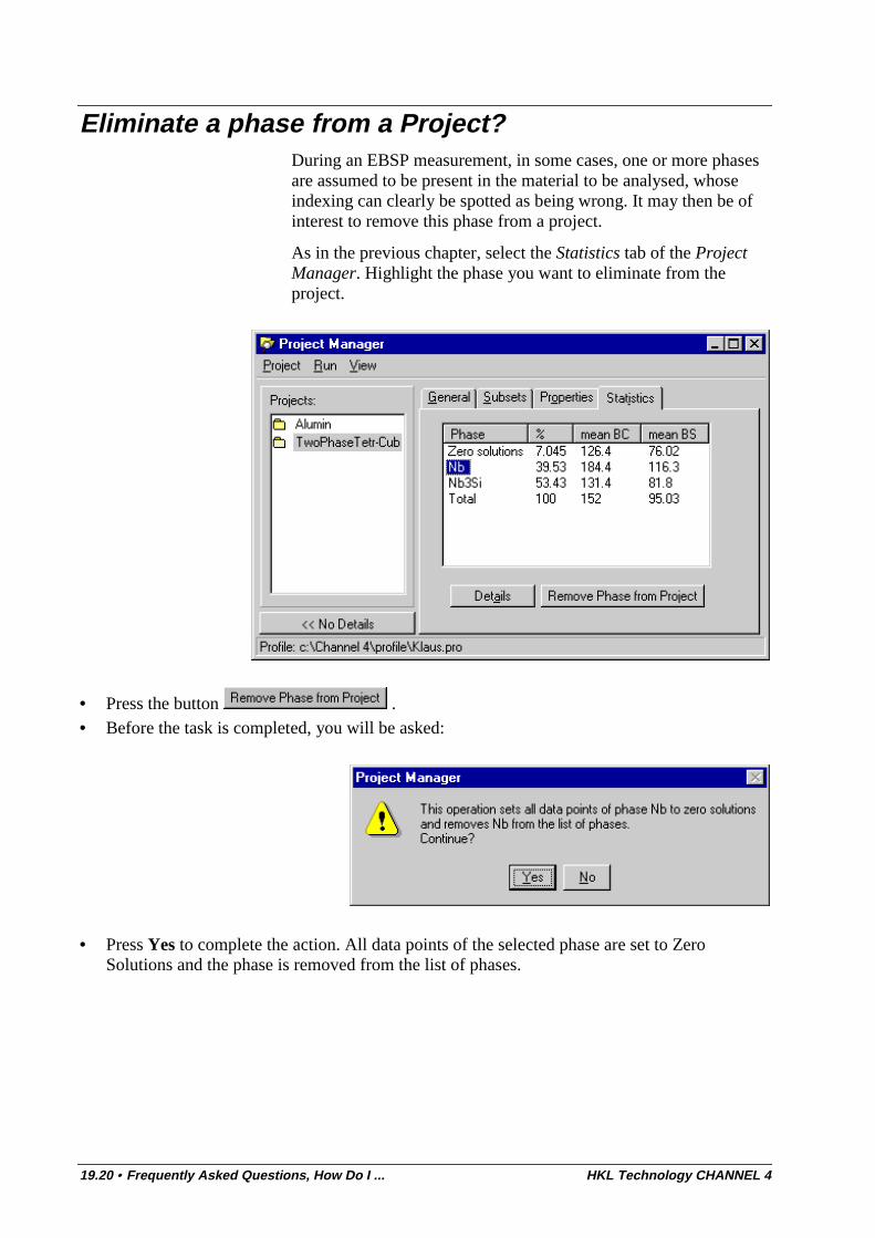
19.20 • Frequently Asked Questions, How Do I ... HKL Technology CHANNEL 4
Eliminate a phase from a Project?During an EBSP measurement, in some cases, one or more phasesare assumed to be present in the material to be analysed, whoseindexing can clearly be spotted as being wrong. It may then be ofinterest to remove this phase from a project.
As in the previous chapter, select the Statistics tab of the ProjectManager. Highlight the phase you want to eliminate from theproject.
• Press the button .• Before the task is completed, you will be asked:
• Press Yes to complete the action. All data points of the selected phase are set to ZeroSolutions and the phase is removed from the list of phases.
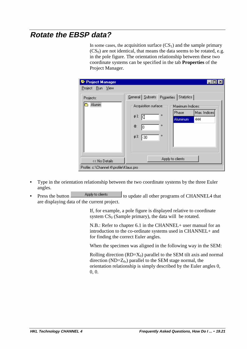
HKL Technology CHANNEL 4 Frequently Asked Questions, How Do I ... • 19.21
Rotate the EBSP data?In some cases, the acquisition surface (CS1) and the sample primary(CS0) are not identical, that means the data seems to be rotated, e.g.in the pole figure. The orientation relationship between these twocoordinate systems can be specified in the tab Properties of theProject Manager.
• Type in the orientation relationship between the two coordinate systems by the three Eulerangles.
• Press the button to update all other programs of CHANNEL4 thatare displaying data of the current project.
If, for example, a pole figure is displayed relative to coordinatesystem CS0 (Sample primary), the data will be rotated.
N.B.: Refer to chapter 6.1 in the CHANNEL+ user manual for anintroduction to the co-ordinate systems used in CHANNEL+ andfor finding the correct Euler angles.
When the specimen was aligned in the following way in the SEM:
Rolling direction (RD=X0) parallel to the SEM tilt axis and normaldirection (ND=Z0,) parallel to the SEM stage normal, theorientation relationship is simply described by the Euler angles 0,0, 0.
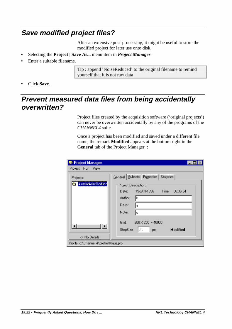
19.22 • Frequently Asked Questions, How Do I ... HKL Technology CHANNEL 4
Save modified project files?After an extensive post-processing, it might be useful to store themodified project for later use onto disk.
• Selecting the Project | Save As... menu item in Project Manager.• Enter a suitable filename.
Tip : append ‘NoiseReduced’ to the original filename to remindyourself that it is not raw data
• Click Save.
Prevent measured data files from being accidentallyoverwritten?
Project files created by the acquisition software (‘original projects’)can never be overwritten accidentally by any of the programs of theCHANNEL4 suite.
Once a project has been modified and saved under a different filename, the remark Modified appears at the bottom right in theGeneral tab of the Project Manager :
HKL Technology CHANNEL 4 Bibliography • 20.1
Bibliography
EBSD measurements and orientation mapping.Bunge, H.J. 1982. Texture Analysis in Materials Science - Mathematical Methods.
Butterworths, London.
Dingley, D.J. & Randle, V. 1992. Microtexture Determination by Electron BackscatterDiffraction. J. Mat. Sci. 27, Vol. 17, 4545-4566.
Engler, O., Gottstein, G. Pospiech, J. & Jura, J. 1994. Statistics, evaluation andrepresentation of single grain orientation measurements. In: Bunge, H.J. [ed.]:Proceedings of the 10th International Conference on Textures of Materials, MaterialsScience Forum 157-162, 259-274.
Humphreys, F.J. 1988. Experimental techniques for microtexture determination. In:Kallend, J.S. & Gottstein, G. [eds.]: Eighth International Conference on Textures ofMaterials (ICOTOM 8), The Metallurgical Society, 171-182.
Humphreys, F.J. 1997. Microtextures by EBSD - some hardware and softwareconsiderations. In: Neumann, B. & Schmidt, N.-H. [eds.]: New applications anddevelopments related to CHANNEL+ and the EBSP technique, Abstract Volume,CHANNEL Users Meeting, Aarhus, Denmark January 1997, 1-3.
Juul Jensen, D. & Schmidt, N.-H. 1990. An Automatic On-Line technique fordetermination of Crystallographic Orientations by EBSP. Recrystallisation ’90, Trans.Met. Soc., 219-224.
Juul Jensen, D. & Schmidt, N.-H. 1991. Local Texture Measurements by EBSP. NewComputer Procedures. Textures & Microstructures 14-18, 92-102.
Randle, V. 1992. Microtexture Determination and its Applications. The Institute ofMetals - No.510, London, ISBN 0-901716 35 9.
Schmidt, N.-H., Bilde-Sørensen, J.B. & Juul Jensen, D. 1991. Scanning Microscopy 5,637.
Venables, J.A. & Harland, C.J. 1973. Electron Backscattering Patterns. Philos. Mag. 27,1193-1200.
Wright, S.I. & Adams, B.L. 1991. Automated lattice orientation determination fromElectron Backscatter Kikuchi diffraction patterns. Textures & Microstructures 14-18,273-278
20.2 • Bibliography HKL Technology CHANNEL 4
Crystal dataInternational Tables for X-ray Crystallography.
Pearson’s Handbook of Crystallographic Data for Intermetallic Phases, ASM, 1991.
Wyckoff, R.W.G. 1968. Crystal Structures, Interscience Publishers, New York.
Introduction to crystallographyBarrett, C, Massalski, T., Structure of Metals, crystallographic methods, principles and
data, Pergamon press, 1980, ISBN 0-08-0216172-8. Chapters 1 & 4.
Battey, M.H., Mineralogy for students, Longman, 1972, ISBN 0 582 44159 5. Capters 1,2 and 5.
Ashcroft, N.W., Mermin, N.D., Solid State Physics, CBS publishing Asia Ltd., 1976,ISBN 0-03-049346-3. Chapters 4-7.
ODFs and texture analysis.Bunge, H.J. 1982. Texture Analysis in Materials Science - Mathematical Methods.
Butterworths, London.
Bunge, H.-J. 1985, Representations of preferred orientations. Wenk (ed.): PreferredOrientation in deformed materials..., Ch. 4
Bunge, H.-J. and C. Esling 1985, The harmonic method. Wenk (ed.): PreferredOrientation in deformed materials..., Ch. 5
Bunge, H.-J. 1985, Physical properties of polycrystals. Wenk (ed.): Preferred Orientationin deformed materials..., Ch. 24
Bunge, H.-J. 1993 (1982), Texture analysis in material science.
Eschner, T. 1997, Orientation distribution functions obtained from Channel+ data. Newapplications and developments related to CHANNEL+ and the EBSP technique. HKLSoftware.
Engler, O., G. Gottstein, J. Pospiech and J. Jura, 1994. Statistics, evaluation andrepresentation of single grain orientation measurements. Materials Science ForumVols. 157-162.
Morris, P.R. and J.W. Flowers 1985, Texture and magnetic properties of metals. Wenk(ed.): Preferred Orientation in deformed materials..., Ch. 25
Pospiech, J., K. Sztwiertnia and F. Haessner 1986. The misorientation distributionfunction. Textures and Microstructures, Vol 6
Wagner, F. 1986. Texture determination by individual orientation measurements. Bunge(ed.): Experimental techniques of texture analysis.
Wenk, H-R, Preferred orientation in deformed metals and rocks: and introduction tomodern texture analysis, Academic press, inc. , 1985, ISBN 0-12-744020-8.
HKL Technology CHANNEL 4 Glossary of terms • 21.1
Glossary of terms
(M)ODFA (Mis) Orientation Distribution Function. (M)ODFs can be calculated using Salsa via theGaussian kernel estimation or Series expansion methods.
À See the sections called Salsa - getting started, Creating an (M)ODF using the (M)ODFwizard and Salsa - introduction to ODF calculations for more information.
Acquisition surfaceThe surface from which the EBSP measurements are acquired, referred to as co-ordinate system1 (CS1).
À See the Glossary entry for Co-ordinate system and Sample primary (CS0).
Axis/angle pairThe most commonly used representation of a misorientation between neighbouring crystallites.The misorientation is represented by a rotation angle ω around a rotation axis (ψ, θ) which iscommon to and brings both crystal co-ordinate systems into coincidence
À See Misorientation profile in Tango - getting started and the Glossary entry forMisorientation.
Band contrast (BC)Band contrast is an image quality factor derived from the Hough transformation which isdescribing the average intensity of the Kikuchi bands with regard to the overall intensity withinthe area of interest (AOI). The values are scaled to the byte range from 0 to 255 (i.e. low to highcontrast).
À For more information see the section called Creating a band contrast and zero solutionmap in Tango – getting started or the section on Grid components in Tango - mapcomponents.
À You can change the way that the Band Contrast map is displayed via Tango’s Legend, seethe section called The map legend in Tango - getting started. Click on the graph and dragto the right to zoom, drag to the left to reset. A right mouse button click gives you accessto Range to subset…, Export, Zoom Histogram…
Band slope (BS)Band slope is an image quality factor derived from the Hough transformation which is describingthe maximum intensity gradient at the margins of the Kikuchi bands in an EBSP. The values are

21.2 • Glossary of terms HKL Technology CHANNEL 4
scaled to the byte range from 0 to 255 (i.e. low to high maximum contrast difference), i.e. thehigher the value, the sharper the image.
À For more information see the section called Grid components in Tango - mapcomponents.
À You can change the way that the Band Slope map is displayed via Tango’s Legend, seethe section called The map legend in Tango - getting started. Click on the graph and dragto the right to zoom, drag to the left to reset. A right mouse button click gives you accessto Range to subset…, Export, Zoom Histogram…
Beam controlAn add-on software module to CHANNEL - acquisition facilitating fully automated EBSP via asoftware-controlled deflection of the electron beam in the SEM.
À See the section called Stage and Beam Jobs in EBSD – getting started for more details..
À See also the glossary entry for Job mode.
Bragg angleThe width of a Kikuchi band (hkl) is twice the Bragg angle, Θ B , for the plane. The Bragg angleis calculated using the equation for the Bragg condition.
Bragg conditionThe Bragg condition, nλ = 2 ⋅dhkl BsinΘ , defines the conditions for diffraction to occur.
Θ B is the Bragg angle,n is an integer and defines the diffraction order, e.g. first.dhkl is the interplanar spacing for the (hkl) plane.λ the wavelength of the incident radiation.
For SEM electrons, the wavelength (Å) is λ ≈0.387
kV, where kV is the accelerating voltage (kV)
N.B. At higher kV, a relativistic correction is required. For SEM electrons this is usually notneeded.
Brandon criterionA criterion which is often used to describe the maximum tolerable deviation from a CSL
boundary given by the expression: vm = °15Σ .
À See CSL boundary in the Glossary.
À In Tango, to define other deviation criteria, select the Components | Componentmanager menu item. Double click on the CSL boundaries component, select the CSLboundaries tab and click on the Deviation button. You can also directly edit thespreadsheet data on the CSL boundaries tab. Double click on Pen entry to change the pensettings. Put a cross in the Show column to enable a particular CSL.
Browser1) In Project manager, a means of browsing EBSD data. Click on View | Record browser.
HKL Technology CHANNEL 4 Glossary of terms • 21.3
2) In Salsa, a means of looking at a section through an (M)ODF. Click on View | Browser or .
À See the sections called Browsing a section through the (M)ODF and Density profile inSalsa - getting started.
3) In Tango, there are Linear intercept and Grain browsers that allow grain measurements to beexamined, e.g. to locate a particular grain.
À See the sections called Grain reconstruction and Line intercept in Tango - gettingstarted for more information. You need to press the Statistics button t reach the browser.
CalibrationIn CHANNEL - acquisition, calibration is the determination of the EBSD geometry. It involvesdetermining the pattern centre (PC), specimen to detector distance (DD), V/H ratio and DetectorOrientation.
À For more information see the sections called Calibration parameters and Calibrationrefinements in EBSD system calibration.
CHANNEL4A suite of programs for measuring and analysing EBSD data. The suite includes : Tango(mapping), Salsa (ODF), Mambo (pole figures), Project Manager, CHANNEL - acquisition.
À See the section called General Introduction for more information.
ClusteringTo speed up the ODF calculations in Salsa, a Clustering of the data can be performed. Thismeans that the Euler space is divided into cells of the size ∆g (the width of these cells isspecified by the parameter Cluster Size (in the tab Clustering of the (M)ODF Parameters dialogbox). Subsequently, the number of measurements ng
falling into each cell is counted. A new data
set is created, expressed by the coordinates of the center of each cell and the weight as n Ng
(‘Clustering’). As a result of this operation, there are usually fewer points to consider. The resultsare only slightly influenced by the Cluster Size, so long as it is not too large.
À See the section called Calculation methods in Salsa - introduction to ODF calculationsfor more information.
Coincidence site latticeThe coincidence site lattice (CSL) describes a 3-D ‘superlattice’ where a specific number oflattice sites from the crystal lattices of two neighbouring grains are superimposed (coincident). ACSL is usually described by the reciprocal density of coincident lattice sites (Σ). E.g. a Σ9 CSLrefers to a coincidence of 1/9 of the lattice sites (or Σ7 - 1/7, Σ5 - 1/5, Σ3 - 1/3, etc.). A Σ1 CSLrefers to a coincidence of all lattice sites, i.e. as in a low-angle boundary. The most common CSLboundaries (e.g. Σ3, Σ9 and Σ27) are twin boundaries.
À See the section called Boundary components in Tango - map components.
À You can get CSL statistics (% of total boundary length) from Tango's Legend, see thesection called The map legend in Tango - getting started. Access it via View | Legend orclick the legend icon, . You'll need to do a right mouse click on the graph and select
21.4 • Glossary of terms HKL Technology CHANNEL 4
Zoom Histogram, then just click on a column for the exact percentage. Another rightmouse click on the Zoomed Histogram gives you Export Data….
ComponentÀ See the Glossary entries for Map component and Texture component
Component libraryA file (*.CMP) containing a selection of pre-defined map components in Tango. Any user-defined selection of map components can be stored and later be loaded as a specific *.CMP file.Accessed using the Components | Load Library…, Components | Save Library andComponents | Save Library As… menu items in Tango.
Component managerA dialog box in Tango to add, remove or edit the map components of a specific componentlibrary. New components can be added and modified from a list of pre-defined component typesand subtypes.
À The shortcut key is F6.
À For more information, see the section called Using map composer - adding componentsin Tango - getting started.
Contoured Pole FigureIn Mambo, a pole figure with a density contouring of the orientation data.
À For more information, see the sections called The Mambo pop-up menus and Displayinga pole figure in Mambo - (inverse) pole figures.
Co-ordinate systemCHANNEL operates with 5 right-handed orthonormal co-ordinate systems. In Tango, Salsa andMambo only CS0 and CS1 are required to specify the orientation relationship between theacquisition surface and the sample primary (the principal sample co-ordinates), i.e. RD, TD andND.
The symbols used to represent the co-ordinate systems are:• CSm (microscope): defined by the microscope axes, i.e. the X-, Y- and Z- stage movement
directions,• CS0 (sample primary): defined by the primary sample axes, e.g. rolling, transverse and
normal directions,• CS1 (acquisition surface): defined by the axes of the measured sample surface - from the
perpendicular edges of a corner,• CS2 (crystal co-ordinate system): defined by the crystal axes, e.g. the [100], [010] and [001]
crystal directions,• CS3 (detector): defined by the detector / diffraction pattern - points on the imaged EBSP are
described by the X- and Y- axes. The Z- axis points out of the phosphor.The axes of each co-ordinate system are termed accordingly, e.g. the microscope axes arerepresented by the co-ordinates Xm, Ym and Zm; and the diffraction pattern by X3, Y3 and Z3. Theposition of the origins of the various co-ordinate systems relative to each other are not needed,for orientation measurement it is the directions that are important.
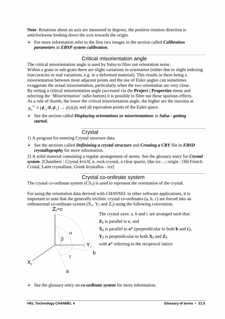
HKL Technology CHANNEL 4 Glossary of terms • 21.5
Note: Rotations about an axis are measured in degrees, the positive rotation direction isanticlockwise looking down the axis towards the origin.
À For more information refer to the first two images in the section called Calibrationparameters in EBSP system calibration.
Critical misorientation angleThe critical misorientation angle is used by Salsa to filter out orientation noise.Within a grain or sub-grain there are slight variations in orientation (either due to slight indexinginaccuracies or real variations, e.g. in a deformed material). This results in there being amisorientation between most adjacent points and the use of Euler angles can sometimesexaggerate the actual misorientation, particularly when the two orientation are very close.By setting a critical misorientation angle (accessed via the Project | Properties menu andselecting the ‘Misorientation’ radio button) it is possible to filter out these spurious effects.As a rule of thumb, the lower the critical misorientation angle, the higher are the maxima at
gijm = →( , , ) ( , , )ϕ ϕ1 2 0 0 0Φ and all equivalent points of the Euler space.
À See the section called Displaying orientations or misorientations in Salsa - gettingstarted.
Crystal1) A program for entering Crystal structure data.
À See the sections called Definining a crystal structure and Creating a CRY file in EBSDcrystallography for more information.
2) A solid material containing a regular arrangement of atoms. See the glossary entry for Crystalsystem. [Chambers : Crystal kris’tl, n. rock-crystal, a clear quartz, like ice…; origin : Old FrenchCristal, Latin crystallum, Greek krystallos - ice]
Crystal co-ordinate systemThe crystal co-ordinate system (CS2) is used to represent the orientation of the crystal.
For using the orientation data derived with CHANNEL in other software applications, it isimportant to note that the generally triclinic crystal co-ordinates (a, b, c) are forced into anorthonormal co-ordinate system (X2, Y2 and Z2) using the following convention.
The crystal axes: a, b and c are arranged such that:
Z2 is parallel to c, and
X2 is parallel to a* (perpendicular to both b and c),
Y2 is perpendicular to both X2 and Z2.
with a* referring to the reciprocal lattice
À See the glossary entry on co-ordinate system for more information.
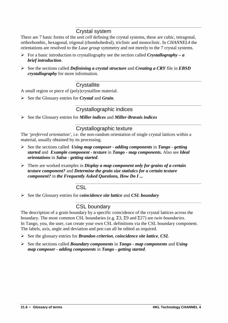
21.6 • Glossary of terms HKL Technology CHANNEL 4
Crystal systemThere are 7 basic forms of the unit cell defining the crystal systems, these are cubic, tetragonal,orthorhombic, hexagonal, trigonal (rhombohedral), triclinic and monoclinic. In CHANNEL4 theorientations are resolved to the Laue group symmetry and not merely to the 7 crystal systems.
À For a basic introduction to crystallography see the section called Crystallography – abrief introduction.
À See the sections called Definining a crystal structure and Creating a CRY file in EBSDcrystallography for more information.
CrystalliteA small region or piece of (poly)crystalline material.
À See the Glossary entries for Crystal and Grain.
Crystallographic indicesÀ See the Glossary entries for Miller indices and Miller-Bravais indices
Crystallographic textureThe ‘preferred orientation’, i.e. the non-random orientation of single crystal lattices within amaterial, usually obtained by its processing.
À See the sections called Using map composer - adding components in Tango - gettingstarted and Example component - texture in Tango - map components. Also see Idealorientations in Salsa - getting started.
À There are worked examples in Display a map component only for grains of a certaintexture component? and Determine the grain size statistics for a certain texturecomponent? in the Frequently Asked Questions, How Do I ...
CSLÀ See the Glossary entries for coincidence site lattice and CSL boundary
CSL boundaryThe description of a grain boundary by a specific coincidence of the crystal lattices across theboundary. The most common CSL boundaries (e.g. Σ3, Σ9 and Σ27) are twin boundaries.In Tango, you, the user, can create your own CSL definitions via the CSL boundary component.The labels, axis, angle and deviation and pen can all be edited as required.
À See the glossary entries for Brandon criterion, coincidence site lattice, CSL
À See the sections called Boundary components in Tango - map components and Usingmap composer - adding components in Tango - getting started.
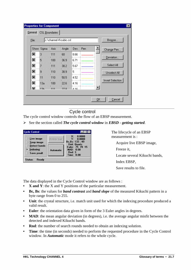
HKL Technology CHANNEL 4 Glossary of terms • 21.7
Cycle controlThe cycle control window controls the flow of an EBSP measurement.
À See the section called The cycle control window in EBSD - getting started.
The lifecycle of an EBSPmeasurement is :
Acquire live EBSP image,
Freeze it,
Locate several Kikuchi bands,
Index EBSP,
Save results to file.
The data displayed in the Cycle Control window are as follows :• X and Y: the X and Y positions of the particular measurement.
• Bc, Bs: the values for band contrast and band slope of the measured Kikuchi pattern in abyte range from 0 to 255.
• Unit: the crystal structure, i.e. match unit used for which the indexing procedure produced avalid result.
• Euler: the orientation data given in form of the 3 Euler angles in degrees.
• MAD: the mean angular deviation (in degrees), i.e. the average angular misfit between thedetected and indexed Kikuchi bands.
• Rnd: the number of search rounds needed to obtain an indexing solution.
• Time: the time (in seconds) needed to perform the requested procedure in the Cycle Controlwindow. In Automatic mode it refers to the whole cycle.
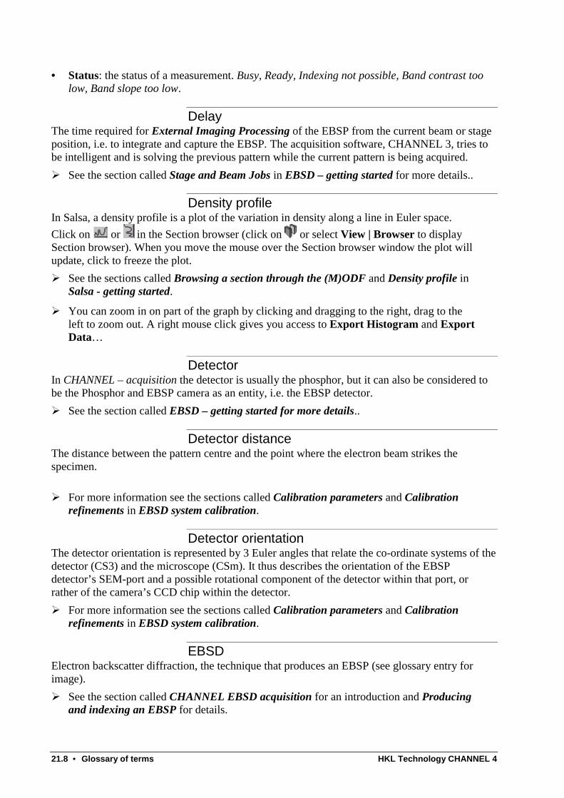
21.8 • Glossary of terms HKL Technology CHANNEL 4
• Status: the status of a measurement. Busy, Ready, Indexing not possible, Band contrast toolow, Band slope too low.
DelayThe time required for External Imaging Processing of the EBSP from the current beam or stageposition, i.e. to integrate and capture the EBSP. The acquisition software, CHANNEL 3, tries tobe intelligent and is solving the previous pattern while the current pattern is being acquired.
À See the section called Stage and Beam Jobs in EBSD – getting started for more details..
Density profileIn Salsa, a density profile is a plot of the variation in density along a line in Euler space.
Click on or in the Section browser (click on or select View | Browser to displaySection browser). When you move the mouse over the Section browser window the plot willupdate, click to freeze the plot.
À See the sections called Browsing a section through the (M)ODF and Density profile inSalsa - getting started.
À You can zoom in on part of the graph by clicking and dragging to the right, drag to theleft to zoom out. A right mouse click gives you access to Export Histogram and ExportData…
DetectorIn CHANNEL – acquisition the detector is usually the phosphor, but it can also be considered tobe the Phosphor and EBSP camera as an entity, i.e. the EBSP detector.
À See the section called EBSD – getting started for more details..
Detector distanceThe distance between the pattern centre and the point where the electron beam strikes thespecimen.
À For more information see the sections called Calibration parameters and Calibrationrefinements in EBSD system calibration.
Detector orientationThe detector orientation is represented by 3 Euler angles that relate the co-ordinate systems of thedetector (CS3) and the microscope (CSm). It thus describes the orientation of the EBSPdetector’s SEM-port and a possible rotational component of the detector within that port, orrather of the camera’s CCD chip within the detector.
À For more information see the sections called Calibration parameters and Calibrationrefinements in EBSD system calibration.
EBSDElectron backscatter diffraction, the technique that produces an EBSP (see glossary entry forimage).
À See the section called CHANNEL EBSD acquisition for an introduction and Producingand indexing an EBSP for details.
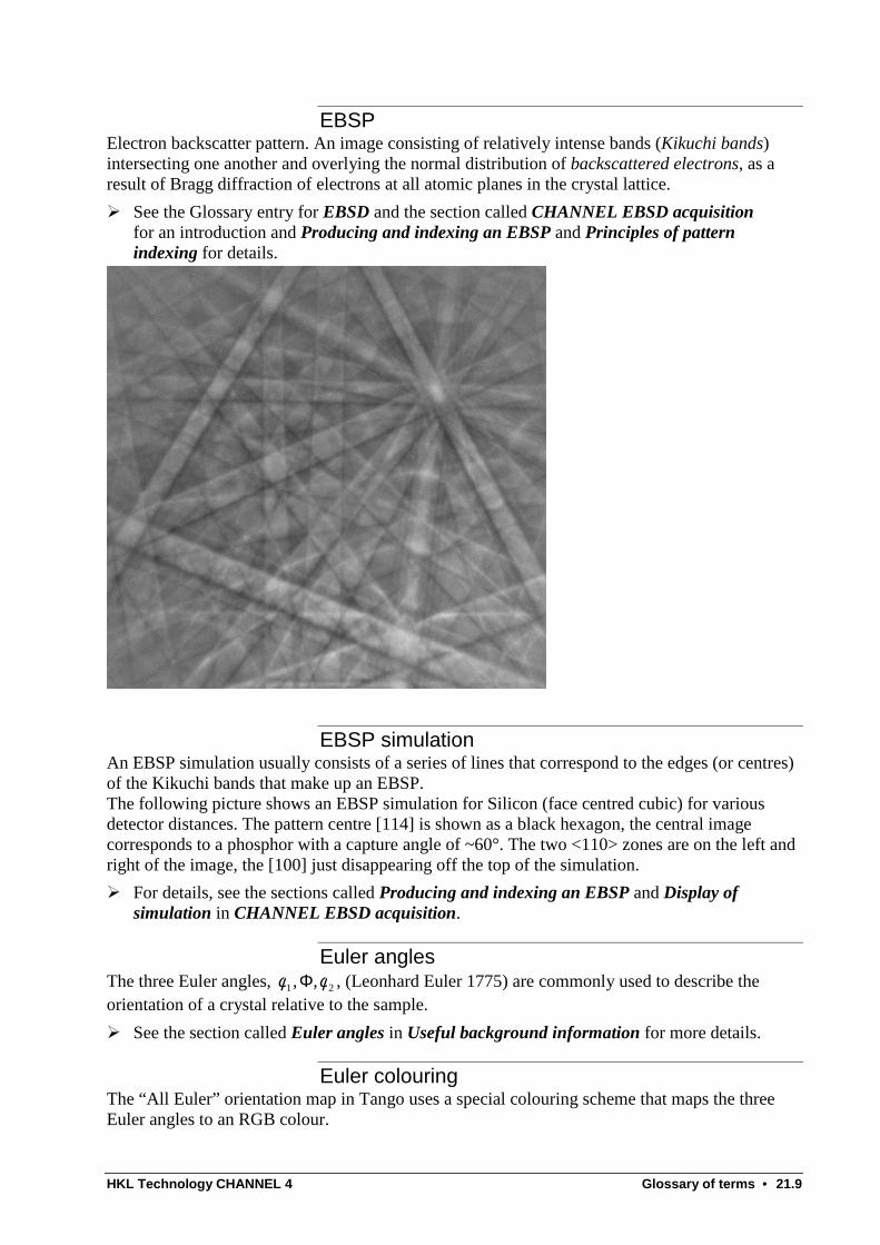
HKL Technology CHANNEL 4 Glossary of terms • 21.9
EBSPElectron backscatter pattern. An image consisting of relatively intense bands (Kikuchi bands)intersecting one another and overlying the normal distribution of backscattered electrons, as aresult of Bragg diffraction of electrons at all atomic planes in the crystal lattice.
À See the Glossary entry for EBSD and the section called CHANNEL EBSD acquisitionfor an introduction and Producing and indexing an EBSP and Principles of patternindexing for details.
EBSP simulationAn EBSP simulation usually consists of a series of lines that correspond to the edges (or centres)of the Kikuchi bands that make up an EBSP.The following picture shows an EBSP simulation for Silicon (face centred cubic) for variousdetector distances. The pattern centre [114] is shown as a black hexagon, the central imagecorresponds to a phosphor with a capture angle of ~60°. The two <110> zones are on the left andright of the image, the [100] just disappearing off the top of the simulation.
À For details, see the sections called Producing and indexing an EBSP and Display ofsimulation in CHANNEL EBSD acquisition.
Euler anglesThe three Euler angles, 21 ,, φφ Φ , (Leonhard Euler 1775) are commonly used to describe theorientation of a crystal relative to the sample.
À See the section called Euler angles in Useful background information for more details.
Euler colouringThe “All Euler” orientation map in Tango uses a special colouring scheme that maps the threeEuler angles to an RGB colour.
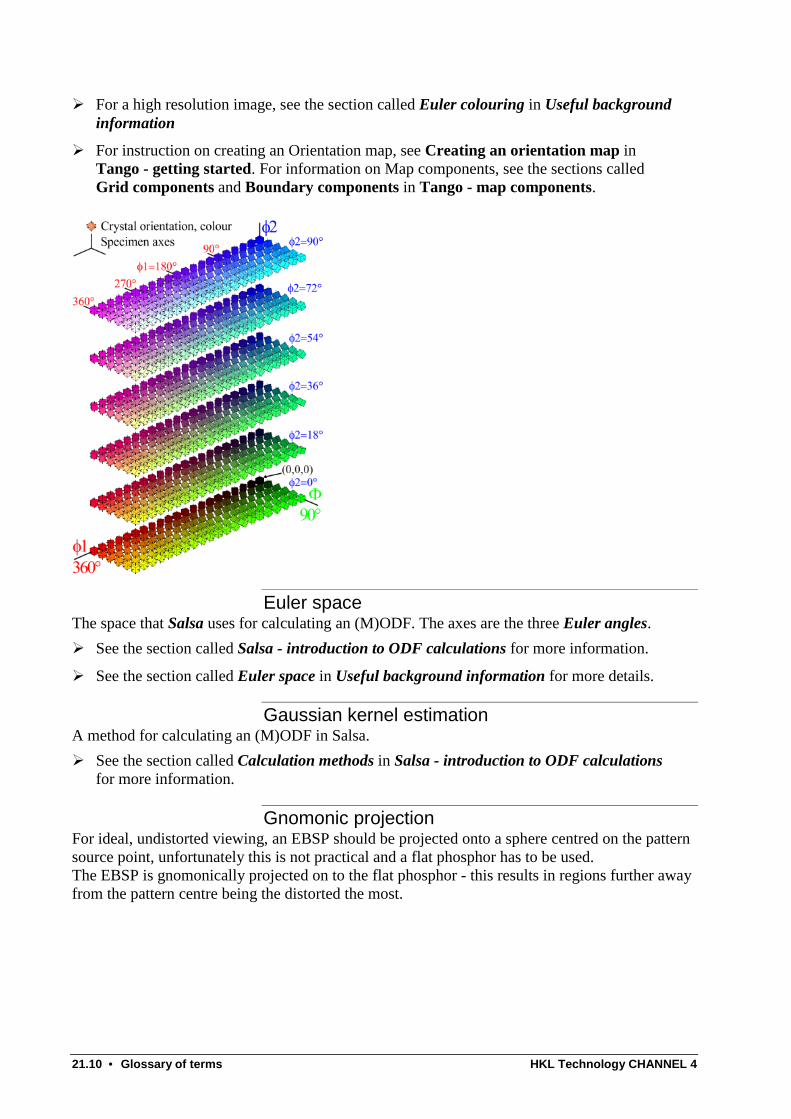
21.10 • Glossary of terms HKL Technology CHANNEL 4
À For a high resolution image, see the section called Euler colouring in Useful backgroundinformation
À For instruction on creating an Orientation map, see Creating an orientation map inTango - getting started. For information on Map components, see the sections calledGrid components and Boundary components in Tango - map components.
Euler spaceThe space that Salsa uses for calculating an (M)ODF. The axes are the three Euler angles.
À See the section called Salsa - introduction to ODF calculations for more information.
À See the section called Euler space in Useful background information for more details.
Gaussian kernel estimationA method for calculating an (M)ODF in Salsa.
À See the section called Calculation methods in Salsa - introduction to ODF calculationsfor more information.
Gnomonic projectionFor ideal, undistorted viewing, an EBSP should be projected onto a sphere centred on the patternsource point, unfortunately this is not practical and a flat phosphor has to be used.The EBSP is gnomonically projected on to the flat phosphor - this results in regions further awayfrom the pattern centre being the distorted the most.
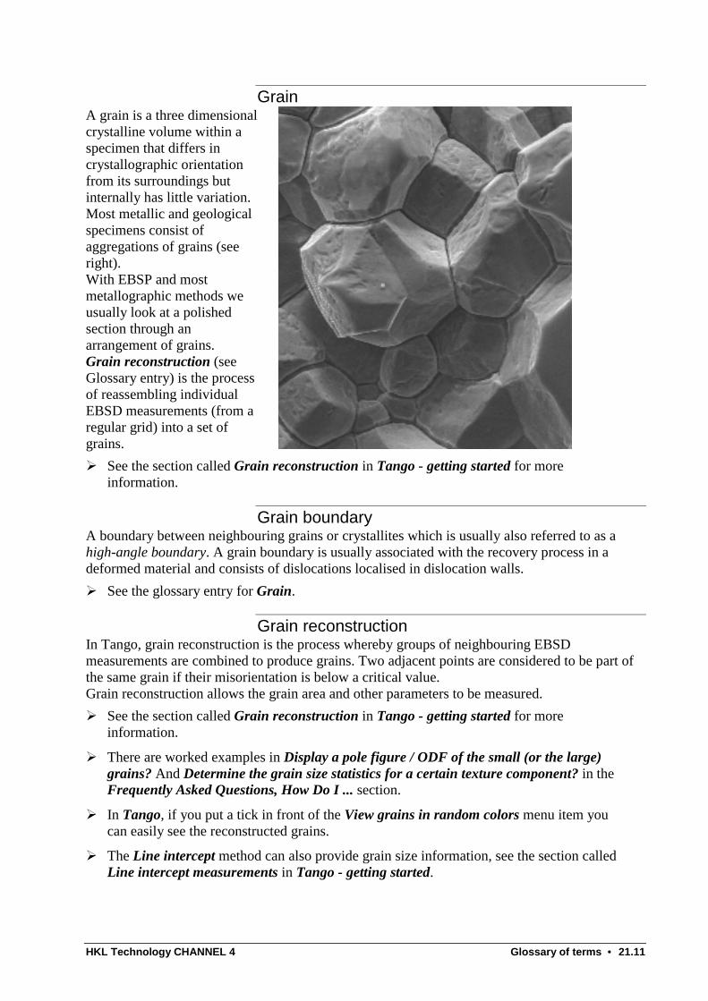
HKL Technology CHANNEL 4 Glossary of terms • 21.11
GrainA grain is a three dimensionalcrystalline volume within aspecimen that differs incrystallographic orientationfrom its surroundings butinternally has little variation.Most metallic and geologicalspecimens consist ofaggregations of grains (seeright).With EBSP and mostmetallographic methods weusually look at a polishedsection through anarrangement of grains.Grain reconstruction (seeGlossary entry) is the processof reassembling individualEBSD measurements (from aregular grid) into a set ofgrains.
À See the section called Grain reconstruction in Tango - getting started for moreinformation.
Grain boundaryA boundary between neighbouring grains or crystallites which is usually also referred to as ahigh-angle boundary. A grain boundary is usually associated with the recovery process in adeformed material and consists of dislocations localised in dislocation walls.
À See the glossary entry for Grain.
Grain reconstructionIn Tango, grain reconstruction is the process whereby groups of neighbouring EBSDmeasurements are combined to produce grains. Two adjacent points are considered to be part ofthe same grain if their misorientation is below a critical value.Grain reconstruction allows the grain area and other parameters to be measured.
À See the section called Grain reconstruction in Tango - getting started for moreinformation.
À There are worked examples in Display a pole figure / ODF of the small (or the large)grains? And Determine the grain size statistics for a certain texture component? in theFrequently Asked Questions, How Do I ... section.
À In Tango, if you put a tick in front of the View grains in random colors menu item youcan easily see the reconstructed grains.
À The Line intercept method can also provide grain size information, see the section calledLine intercept measurements in Tango - getting started.
21.12 • Glossary of terms HKL Technology CHANNEL 4
High-angle boundaryA boundary in a crystalline material which is described by a high-angle misorientation betweenthe neighbouring crystallites, i.e. grains. It is often also referred to as a grain boundary. (see alsolow-angle boundary, subgrain boundary). Depending on the investigated material, a high-angleboundary is defined by a smallest rotation angle (ωmin) above 5°-15°.
À See the glossary entries for Grain, Grain boundary and Grain reconstruction.
HKL TechnologyA Danish company that develops and sells completeEBSD systems. HKL Technology was founded byNiels-Henrik Schmidt.
Address :HKL Technology ApS,Blåkildevej 17k,DK-9500,Hobro,Denmark.
Tel. : +45 96 57 26 00; Fax. : +45 96 57 26 09E-mail : [email protected] : www.channel.dk
Hough transformationThe automated detection of Kikuchi bands in CHANNEL - acquisition is based on a Houghtransformation.The Hough transform maps the EBSP image (X,Y) into Hough space (“theta”, “distance”) bycalculating the average intensity along lines inclined at an angle “theta” and displaced from thecentre of the image by “distance”. A point in the EBSP transforms into a sinusoid in Houghspace, a thin line transforms into a point. A Kikuchi band of width d transforms into a pair oflocal maxima (or minima) that are separated by a distance d. A butterfly filter is used to identifythese maxima.
À See the section called Indexing patterns and Critical choice of cycle control parametersin EBSP - running an experiment.
À For the original details, see Paul V.C. Hough; U.S. Patent 3,069,654; Dec. 18, 1962;Method and Means for Recognizing Complex Patterns
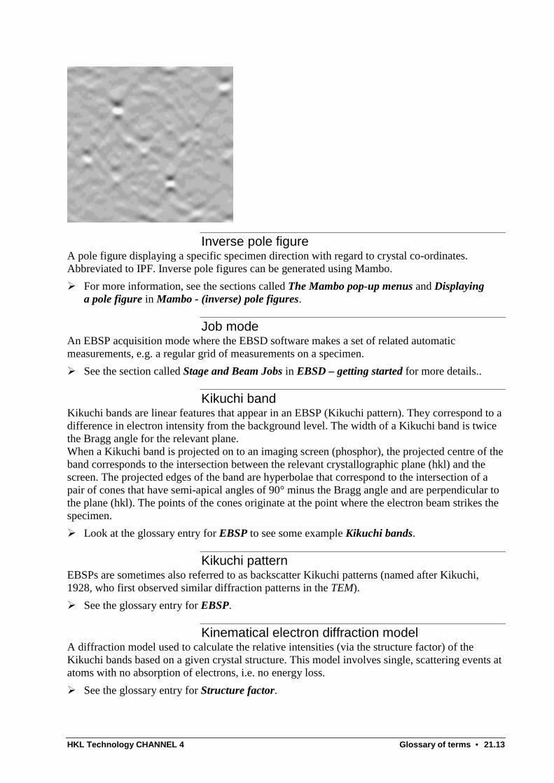
HKL Technology CHANNEL 4 Glossary of terms • 21.13
Inverse pole figureA pole figure displaying a specific specimen direction with regard to crystal co-ordinates.Abbreviated to IPF. Inverse pole figures can be generated using Mambo.
À For more information, see the sections called The Mambo pop-up menus and Displayinga pole figure in Mambo - (inverse) pole figures.
Job modeAn EBSP acquisition mode where the EBSD software makes a set of related automaticmeasurements, e.g. a regular grid of measurements on a specimen.
À See the section called Stage and Beam Jobs in EBSD – getting started for more details..
Kikuchi bandKikuchi bands are linear features that appear in an EBSP (Kikuchi pattern). They correspond to adifference in electron intensity from the background level. The width of a Kikuchi band is twicethe Bragg angle for the relevant plane.When a Kikuchi band is projected on to an imaging screen (phosphor), the projected centre of theband corresponds to the intersection between the relevant crystallographic plane (hkl) and thescreen. The projected edges of the band are hyperbolae that correspond to the intersection of apair of cones that have semi-apical angles of 90° minus the Bragg angle and are perpendicular tothe plane (hkl). The points of the cones originate at the point where the electron beam strikes thespecimen.
À Look at the glossary entry for EBSP to see some example Kikuchi bands.
Kikuchi patternEBSPs are sometimes also referred to as backscatter Kikuchi patterns (named after Kikuchi,1928, who first observed similar diffraction patterns in the TEM).
À See the glossary entry for EBSP.
Kinematical electron diffraction modelA diffraction model used to calculate the relative intensities (via the structure factor) of theKikuchi bands based on a given crystal structure. This model involves single, scattering events atatoms with no absorption of electrons, i.e. no energy loss.
À See the glossary entry for Structure factor.
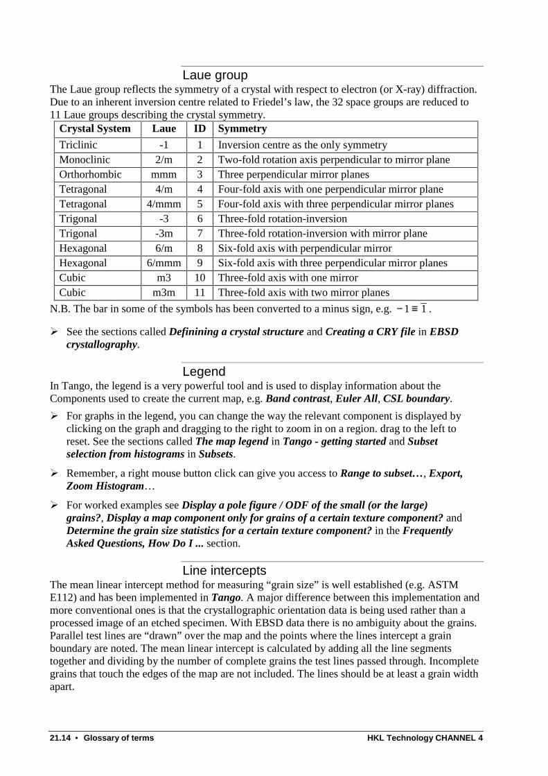
21.14 • Glossary of terms HKL Technology CHANNEL 4
Laue groupThe Laue group reflects the symmetry of a crystal with respect to electron (or X-ray) diffraction.Due to an inherent inversion centre related to Friedel’s law, the 32 space groups are reduced to11 Laue groups describing the crystal symmetry.
Crystal System Laue ID Symmetry
Triclinic -1 1 Inversion centre as the only symmetryMonoclinic 2/m 2 Two-fold rotation axis perpendicular to mirror planeOrthorhombic mmm 3 Three perpendicular mirror planesTetragonal 4/m 4 Four-fold axis with one perpendicular mirror planeTetragonal 4/mmm 5 Four-fold axis with three perpendicular mirror planesTrigonal -3 6 Three-fold rotation-inversionTrigonal -3m 7 Three-fold rotation-inversion with mirror planeHexagonal 6/m 8 Six-fold axis with perpendicular mirrorHexagonal 6/mmm 9 Six-fold axis with three perpendicular mirror planesCubic m3 10 Three-fold axis with one mirrorCubic m3m 11 Three-fold axis with two mirror planes
N.B. The bar in some of the symbols has been converted to a minus sign, e.g. − ≡1 1 .
À See the sections called Definining a crystal structure and Creating a CRY file in EBSDcrystallography.
LegendIn Tango, the legend is a very powerful tool and is used to display information about theComponents used to create the current map, e.g. Band contrast, Euler All, CSL boundary.
À For graphs in the legend, you can change the way the relevant component is displayed byclicking on the graph and dragging to the right to zoom in on a region. drag to the left toreset. See the sections called The map legend in Tango - getting started and Subsetselection from histograms in Subsets.
À Remember, a right mouse button click can give you access to Range to subset…, Export,Zoom Histogram…
À For worked examples see Display a pole figure / ODF of the small (or the large)grains?, Display a map component only for grains of a certain texture component? andDetermine the grain size statistics for a certain texture component? in the FrequentlyAsked Questions, How Do I ... section.
Line interceptsThe mean linear intercept method for measuring “grain size” is well established (e.g. ASTME112) and has been implemented in Tango. A major difference between this implementation andmore conventional ones is that the crystallographic orientation data is being used rather than aprocessed image of an etched specimen. With EBSD data there is no ambiguity about the grains.Parallel test lines are “drawn” over the map and the points where the lines intercept a grainboundary are noted. The mean linear intercept is calculated by adding all the line segmentstogether and dividing by the number of complete grains the test lines passed through. Incompletegrains that touch the edges of the map are not included. The lines should be at least a grain widthapart.
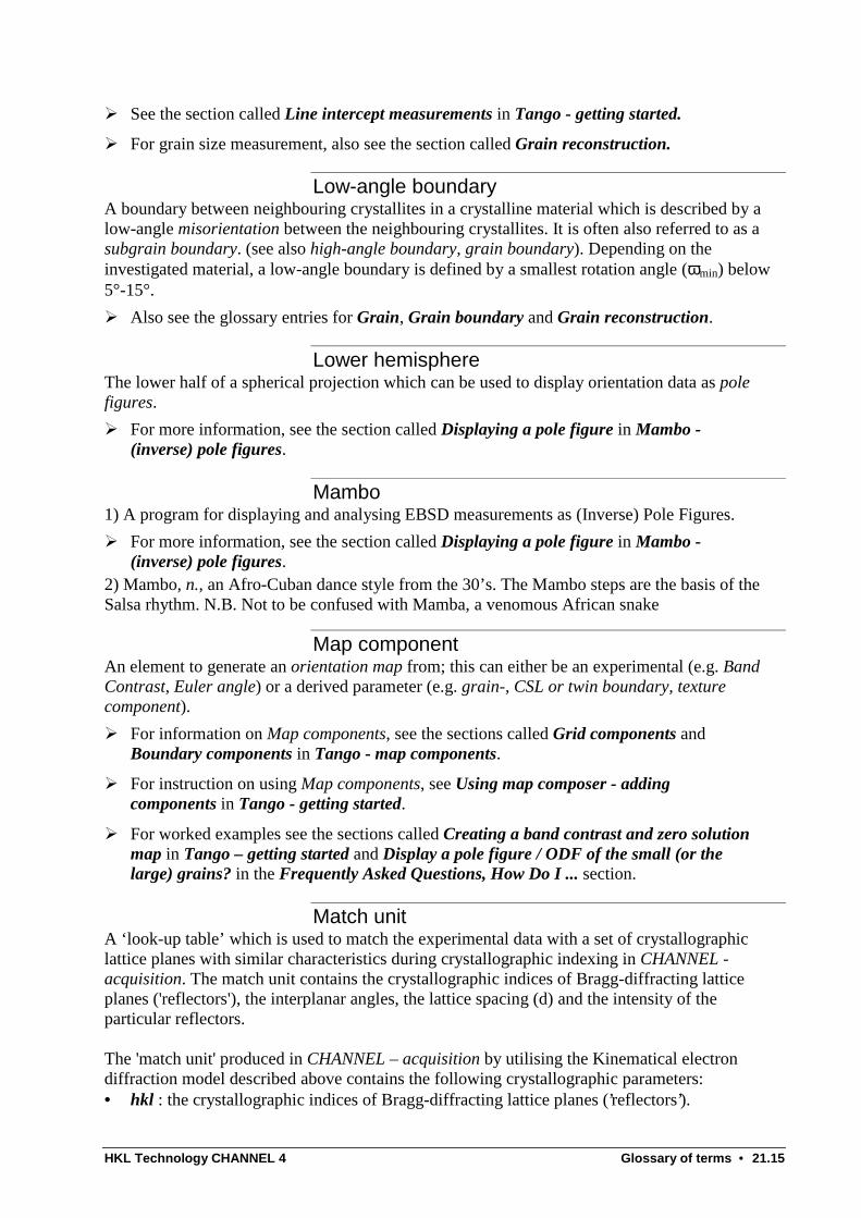
HKL Technology CHANNEL 4 Glossary of terms • 21.15
À See the section called Line intercept measurements in Tango - getting started.
À For grain size measurement, also see the section called Grain reconstruction.
Low-angle boundaryA boundary between neighbouring crystallites in a crystalline material which is described by alow-angle misorientation between the neighbouring crystallites. It is often also referred to as asubgrain boundary. (see also high-angle boundary, grain boundary). Depending on theinvestigated material, a low-angle boundary is defined by a smallest rotation angle (ωmin) below5°-15°.
À Also see the glossary entries for Grain, Grain boundary and Grain reconstruction.
Lower hemisphereThe lower half of a spherical projection which can be used to display orientation data as polefigures.
À For more information, see the section called Displaying a pole figure in Mambo -(inverse) pole figures.
Mambo1) A program for displaying and analysing EBSD measurements as (Inverse) Pole Figures.
À For more information, see the section called Displaying a pole figure in Mambo -(inverse) pole figures.
2) Mambo, n., an Afro-Cuban dance style from the 30’s. The Mambo steps are the basis of theSalsa rhythm. N.B. Not to be confused with Mamba, a venomous African snake
Map componentAn element to generate an orientation map from; this can either be an experimental (e.g. BandContrast, Euler angle) or a derived parameter (e.g. grain-, CSL or twin boundary, texturecomponent).
À For information on Map components, see the sections called Grid components andBoundary components in Tango - map components.
À For instruction on using Map components, see Using map composer - addingcomponents in Tango - getting started.
À For worked examples see the sections called Creating a band contrast and zero solutionmap in Tango – getting started and Display a pole figure / ODF of the small (or thelarge) grains? in the Frequently Asked Questions, How Do I ... section.
Match unitA ‘look-up table’ which is used to match the experimental data with a set of crystallographiclattice planes with similar characteristics during crystallographic indexing in CHANNEL -acquisition. The match unit contains the crystallographic indices of Bragg-diffracting latticeplanes ('reflectors'), the interplanar angles, the lattice spacing (d) and the intensity of theparticular reflectors.
The 'match unit' produced in CHANNEL – acquisition by utilising the Kinematical electrondiffraction model described above contains the following crystallographic parameters:• hkl : the crystallographic indices of Bragg-diffracting lattice planes (’reflectors’).

21.16 • Glossary of terms HKL Technology CHANNEL 4
• dhkl : the lattice plane spacing of the particular reflectors.
• nhkl : the normal vectors to the reflectors.
• Ihkl : the intensity of the reflectors.
• ∠n ni j; : the interplanar angles between the reflectors.
From these parameters the interplanar angles ( ∠n ni j; ) are primarily used for indexing. Thelattice plane spacing ( dhkl ) can optionally be applied, whereas the intensity of the reflectors ( Ihkl )is only used as a threshold value to select the number of reflectors in the match unit.
À For information on creating a Match unit, see the sections called Creating a match unit,Critical choice of reflectors used in the match unit and Principles of pattern indexing inEBSD crystallography.
À For information on creating a .CRY file, see the sections called Defining a crystalstructure and Creating a CRY file in EBSD crystallography.
Mean angular deviationA number which expresses how well the simulated EBSP overlays the actual EBSP. The MAD isgiven in degrees specifying the averaged angular misfit between detected and simulated Kikuchibands.
À See the Cycle control Glossary entry.
Mean linear interceptÀ See the glossary entry for Line intercept
Miller indicesThe 3-digit crystallographic indices used to describe crystallographic lattice planes (hkl) ordirections [uvw].
Miller-Bravais indicesThe 4-digit crystallographic indices used to describe crystallographic lattice planes (hkil) ordirections [uvtw] in the hexagonal and trigonal crystal systems.
MisorientationDescribes the orientation difference between two grains in terms of a rotation of their crystal co-ordinate systems into coincidence. This rotation may be described in the form of Euler angles,Rodriguez vectors or in the most common form as ‘rotation axis/angle pairs’. Depending on thecrystal symmetry different crystallographically equivalent rotation axis/angle pairs exist todescribe this rotation (e.g. 24 for cubic, 12 for hexagonal, 6 for trigonal symmetry). Byconvention the rotation axis/angle pair with the smallest rotation angle ωmin is used to describe amisorientation.The misorientation gij
m is calculated between the orientation gi
of a grid point and its nearest
neighbour g j (two per point, one to the right and one below) using the following equation:
g g gijm
i j= −1.
À See Misorientation profile in Tango - getting started.
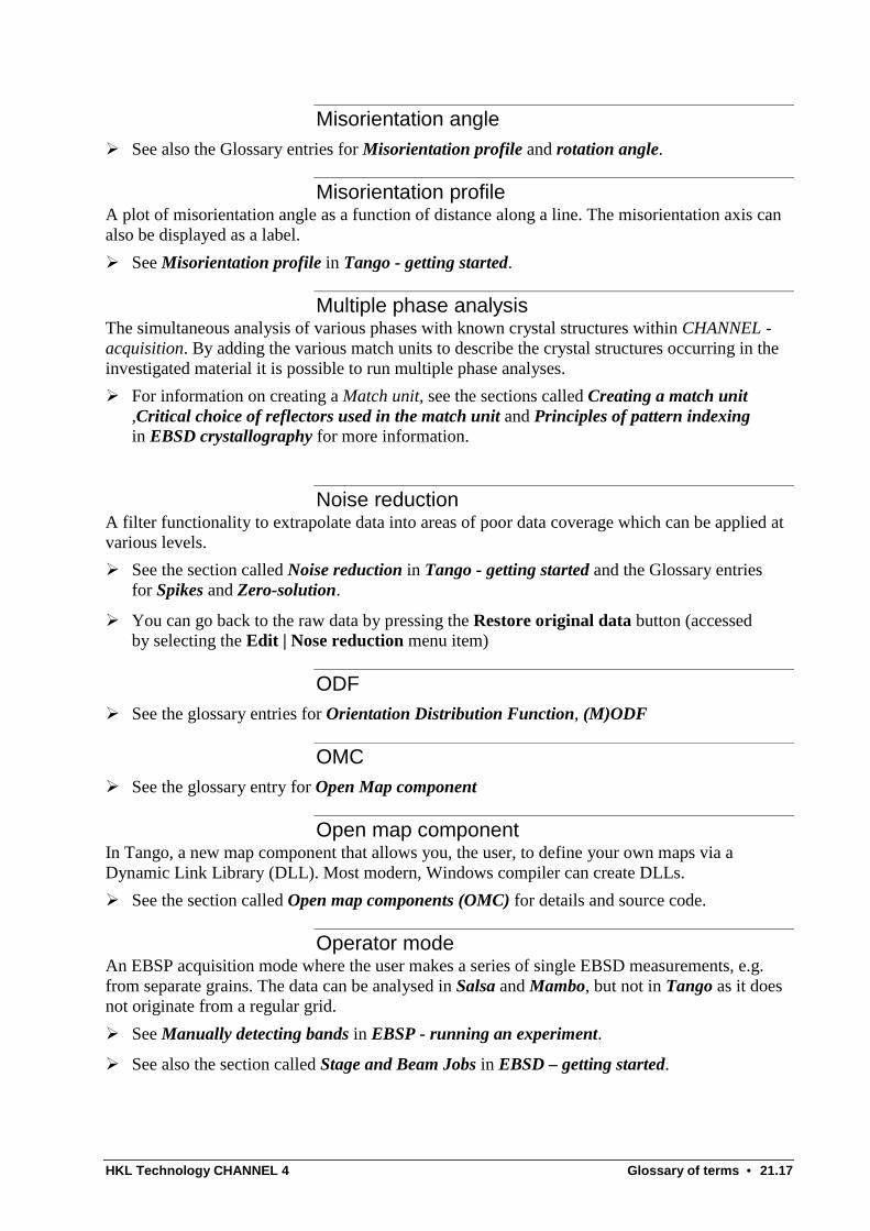
HKL Technology CHANNEL 4 Glossary of terms • 21.17
Misorientation angleÀ See also the Glossary entries for Misorientation profile and rotation angle.
Misorientation profileA plot of misorientation angle as a function of distance along a line. The misorientation axis canalso be displayed as a label.
À See Misorientation profile in Tango - getting started.
Multiple phase analysisThe simultaneous analysis of various phases with known crystal structures within CHANNEL -acquisition. By adding the various match units to describe the crystal structures occurring in theinvestigated material it is possible to run multiple phase analyses.
À For information on creating a Match unit, see the sections called Creating a match unit,Critical choice of reflectors used in the match unit and Principles of pattern indexingin EBSD crystallography for more information.
Noise reductionA filter functionality to extrapolate data into areas of poor data coverage which can be applied atvarious levels.
À See the section called Noise reduction in Tango - getting started and the Glossary entriesfor Spikes and Zero-solution.
À You can go back to the raw data by pressing the Restore original data button (accessedby selecting the Edit | Nose reduction menu item)
ODFÀ See the glossary entries for Orientation Distribution Function, (M)ODF
OMCÀ See the glossary entry for Open Map component
Open map componentIn Tango, a new map component that allows you, the user, to define your own maps via aDynamic Link Library (DLL). Most modern, Windows compiler can create DLLs.
À See the section called Open map components (OMC) for details and source code.
Operator modeAn EBSP acquisition mode where the user makes a series of single EBSD measurements, e.g.from separate grains. The data can be analysed in Salsa and Mambo, but not in Tango as it doesnot originate from a regular grid.
À See Manually detecting bands in EBSP - running an experiment.
À See also the section called Stage and Beam Jobs in EBSD – getting started.
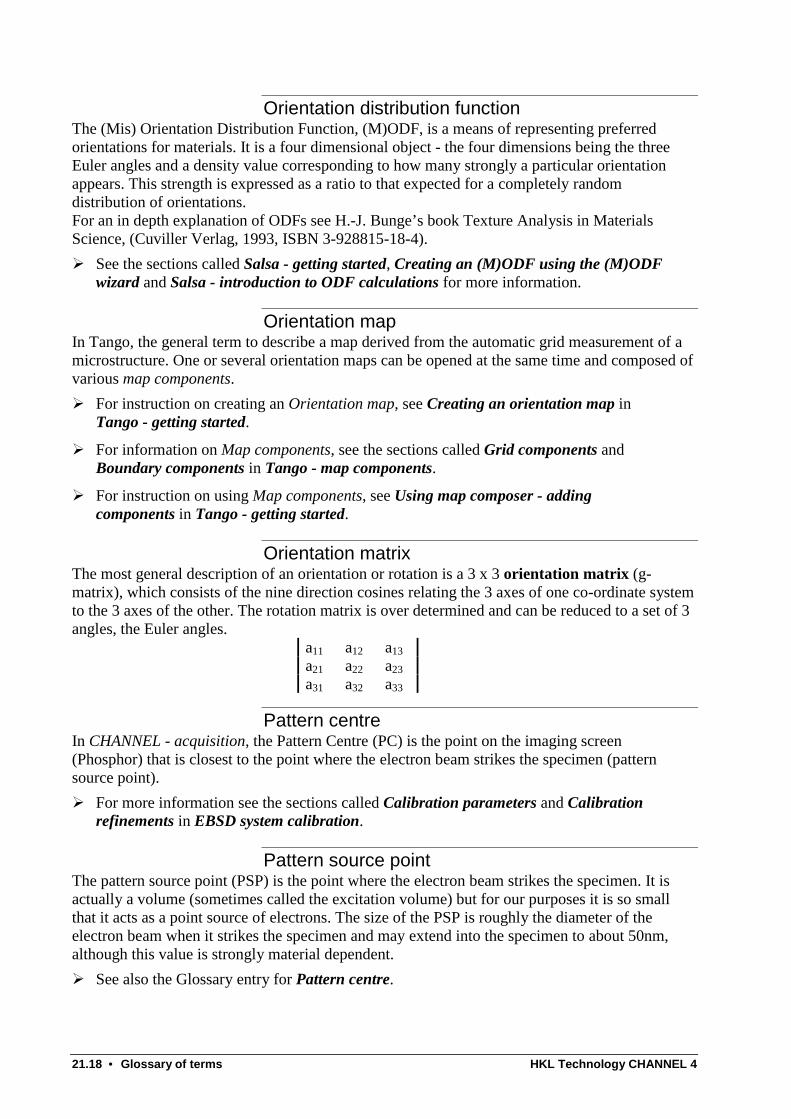
21.18 • Glossary of terms HKL Technology CHANNEL 4
Orientation distribution functionThe (Mis) Orientation Distribution Function, (M)ODF, is a means of representing preferredorientations for materials. It is a four dimensional object - the four dimensions being the threeEuler angles and a density value corresponding to how many strongly a particular orientationappears. This strength is expressed as a ratio to that expected for a completely randomdistribution of orientations.For an in depth explanation of ODFs see H.-J. Bunge’s book Texture Analysis in MaterialsScience, (Cuviller Verlag, 1993, ISBN 3-928815-18-4).
À See the sections called Salsa - getting started, Creating an (M)ODF using the (M)ODFwizard and Salsa - introduction to ODF calculations for more information.
Orientation mapIn Tango, the general term to describe a map derived from the automatic grid measurement of amicrostructure. One or several orientation maps can be opened at the same time and composed ofvarious map components.
À For instruction on creating an Orientation map, see Creating an orientation map inTango - getting started.
À For information on Map components, see the sections called Grid components andBoundary components in Tango - map components.
À For instruction on using Map components, see Using map composer - addingcomponents in Tango - getting started.
Orientation matrixThe most general description of an orientation or rotation is a 3 x 3 orientation matrix (g-matrix), which consists of the nine direction cosines relating the 3 axes of one co-ordinate systemto the 3 axes of the other. The rotation matrix is over determined and can be reduced to a set of 3angles, the Euler angles.
a11 a12 a13
a21 a22 a23
a31 a32 a33
Pattern centreIn CHANNEL - acquisition, the Pattern Centre (PC) is the point on the imaging screen(Phosphor) that is closest to the point where the electron beam strikes the specimen (patternsource point).
À For more information see the sections called Calibration parameters and Calibrationrefinements in EBSD system calibration.
Pattern source pointThe pattern source point (PSP) is the point where the electron beam strikes the specimen. It isactually a volume (sometimes called the excitation volume) but for our purposes it is so smallthat it acts as a point source of electrons. The size of the PSP is roughly the diameter of theelectron beam when it strikes the specimen and may extend into the specimen to about 50nm,although this value is strongly material dependent.
À See also the Glossary entry for Pattern centre.
HKL Technology CHANNEL 4 Glossary of terms • 21.19
PhosphorThe part of the EBSP detector that converts electrons into visible photons and allows EBSPs tobe imaged using a low light level camera (Detector).
À See Glossary entry for Detector.
Pole figureThe spherical projection of crystal directions displayed in a plane representing the upper or lowerhemisphere. Abbreviated to PF.
À For more information, see the sections called The Mambo pop-up menus and Displayinga pole figure in Mambo - (inverse) pole figures.
ProjectThe main file format (.CPR) used by Tango, Mambo, Salsa and Project manager. It is linked tothe actual data stored in a record file (.CRC). Older versions of CHANNEL software use .PRJand .REC files.
À For information on converting data see the section called Convert all of my version 3.1files to the new file format? in Frequently Asked Questions, How Do I ...
Project managerProject manager has overall control of data and can be used to create, manipulate and cominesubsets.
À See the Project manager section.
À You can use the Subsets tab in Project manager (click Details >>) to combine subsetsusing AND, XOR and OR; NOT will swap the subset with the anti-subset and vice versa.See the section called Combining and inverting subsets in Subsets.
PseudosymmetryA pseudosymmetry occurs where two orientations cannot easily be distinguished due to anapparent n-fold rotation axis especially in lower symmetry crystal structures. For example anorthorhombic structure with similar lengths of the a- and b-axis appears to be tetragonal whenviewed down its c-axis, as is the case in some high temperature superconductors. Other examplesof pseudosymmetry are often encountered in geological materials (e.g. pseudohexagonalstructures appearing in trigonal quartz).
À See the section called Pseudosymmetry in EBSP - running an experiment.
Range to subsetRange to subset is a very powerful tool. From the currently selected range of a graph, Range tosubset will put all the EBSD data points that lie within the range in to a new Subset. You can callthe subset anything you want, e.g. squiggly grains.
À See the section called Subset selection from histograms in Subsets and the workedexamples called Display a pole figure / ODF of the small (or the large) grains?, Displaya map component only for grains of a certain texture component? and Determine thegrain size statistics for a certain texture component? in the Frequently AskedQuestions, How Do I ... section.
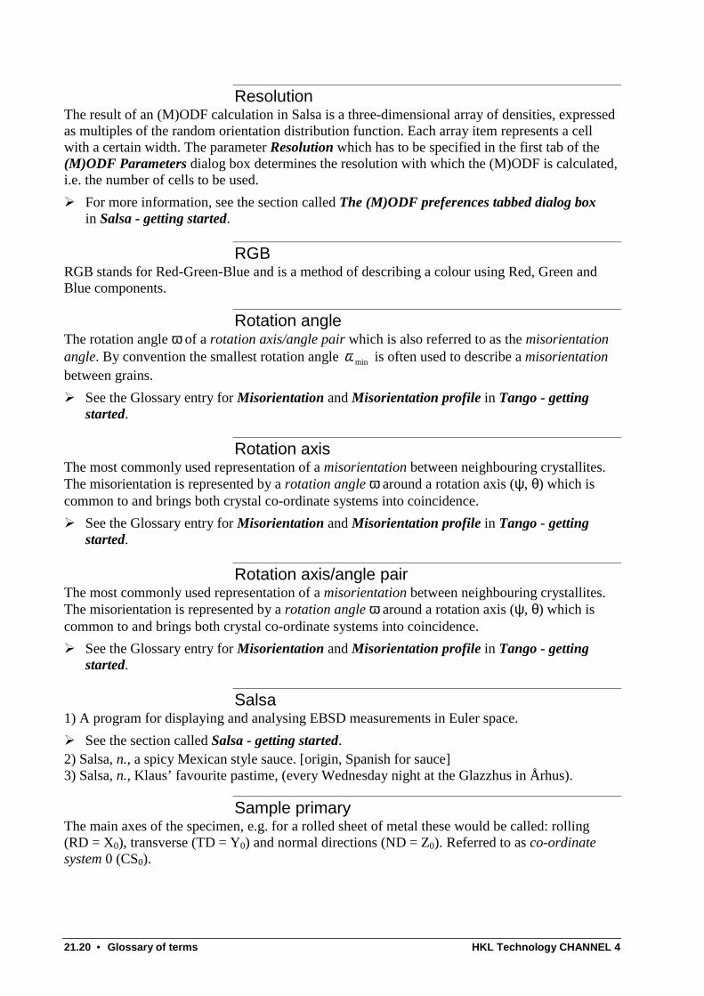
21.20 • Glossary of terms HKL Technology CHANNEL 4
ResolutionThe result of an (M)ODF calculation in Salsa is a three-dimensional array of densities, expressedas multiples of the random orientation distribution function. Each array item represents a cellwith a certain width. The parameter Resolution which has to be specified in the first tab of the(M)ODF Parameters dialog box determines the resolution with which the (M)ODF is calculated,i.e. the number of cells to be used.
À For more information, see the section called The (M)ODF preferences tabbed dialog boxin Salsa - getting started.
RGBRGB stands for Red-Green-Blue and is a method of describing a colour using Red, Green andBlue components.
Rotation angleThe rotation angle ω of a rotation axis/angle pair which is also referred to as the misorientationangle. By convention the smallest rotation angle ω min is often used to describe a misorientationbetween grains.
À See the Glossary entry for Misorientation and Misorientation profile in Tango - gettingstarted.
Rotation axisThe most commonly used representation of a misorientation between neighbouring crystallites.The misorientation is represented by a rotation angle ω around a rotation axis (ψ, θ) which iscommon to and brings both crystal co-ordinate systems into coincidence.
À See the Glossary entry for Misorientation and Misorientation profile in Tango - gettingstarted.
Rotation axis/angle pairThe most commonly used representation of a misorientation between neighbouring crystallites.The misorientation is represented by a rotation angle ω around a rotation axis (ψ, θ) which iscommon to and brings both crystal co-ordinate systems into coincidence.
À See the Glossary entry for Misorientation and Misorientation profile in Tango - gettingstarted.
Salsa1) A program for displaying and analysing EBSD measurements in Euler space.
À See the section called Salsa - getting started.2) Salsa, n., a spicy Mexican style sauce. [origin, Spanish for sauce]3) Salsa, n., Klaus’ favourite pastime, (every Wednesday night at the Glazzhus in Århus).
Sample primaryThe main axes of the specimen, e.g. for a rolled sheet of metal these would be called: rolling(RD = X0), transverse (TD = Y0) and normal directions (ND = Z0). Referred to as co-ordinatesystem 0 (CS0).
HKL Technology CHANNEL 4 Glossary of terms • 21.21
To relate the orientation data derived with CHANNEL to the specimen co-ordinates it isimportant to define the orientation relationship between the sample primary (CS0) and acquisitionsurface (CS1) co-ordinate systems.Since CS1 has been brought into coincidence with the microscope co-ordinate system (CSm) byaligning the specimen surface in the SEM and by taking the tilt angle (usually 70°) into accountin CHANNEL, the orientation relationship between CS0 and CS1 thus allows to correctly rotatethe orientation data with regard to the specimen co-ordinates.The acquisition surface co-ordinate system (CS1) defines the orientation of the sample surface. Inthis co-ordinate system Z1 always refers to the normal of the acquisition surface, whereas X1 andY1 are termed according to their alignment with the microscope axes Xm and Ym. The sampleprimary co-ordinate system (CS0) defines the main axes of the specimen, e.g. for a rolled sheet ofmetal these would be called: rolling (RD = X0), transverse (TD = Y0) and normal directions(ND = Z0).
À For more information refer to the first two images in the section called Calibrationparameters in EBSP system calibration and the glossary entry on co-ordinate system .
Section browserIn Salsa, a tool to allow the viewing of a section through an (M)ODF in Euler space.
Click on View | Browser or .
À See the sections called Browsing a section through the (M)ODF and Density profile inSalsa - getting started.
SEMScanning electron microscope - the source of the electrons that make up and EBSP.CHANNEL – acquisition can control the beam scanning and stage movement on most SEMs.
Serial sectionsIn Salsa, serial sections are a way of looking at sections through an (M)ODF in Euler space.
À See the section called Viewing serial sections through an (M)ODF in Salsa - gettingstarted.
À Click on the Serial section icon, . A right mouse click gives you access to Preferences,Export…
À Select View | Ideal orientations to display a simulated ideal orientation.
Series expansionA method for calculating an (M)ODF in Salsa.
À See the section called Calculation methods in Salsa - introduction to ODF calculationsfor more information.
SpikesSpikes are measurement point with a wrong indexing solution; spikes may occur where no oronly very poor quality EBSP signals are generated, i.e. at grain boundaries, cracks, dislocationclusters, voids, inclusions or around damages on the sample surface.
À See the section called Noise reduction in Tango - getting started.
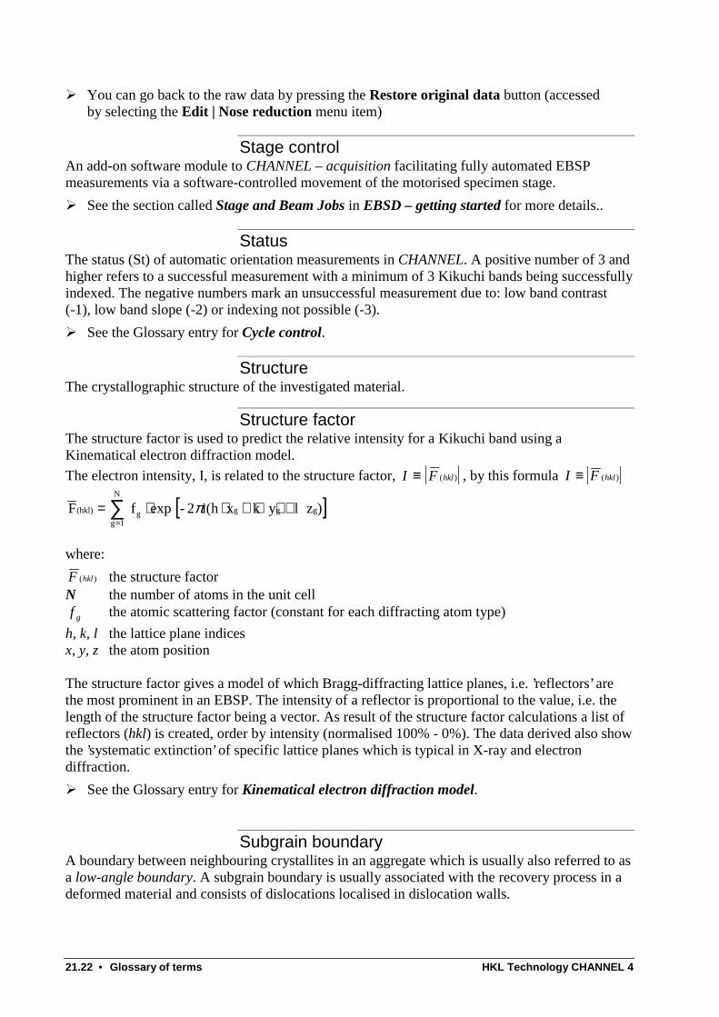
21.22 • Glossary of terms HKL Technology CHANNEL 4
À You can go back to the raw data by pressing the Restore original data button (accessedby selecting the Edit | Nose reduction menu item)
Stage controlAn add-on software module to CHANNEL – acquisition facilitating fully automated EBSPmeasurements via a software-controlled movement of the motorised specimen stage.
À See the section called Stage and Beam Jobs in EBSD – getting started for more details..
StatusThe status (St) of automatic orientation measurements in CHANNEL. A positive number of 3 andhigher refers to a successful measurement with a minimum of 3 Kikuchi bands being successfullyindexed. The negative numbers mark an unsuccessful measurement due to: low band contrast(-1), low band slope (-2) or indexing not possible (-3).
À See the Glossary entry for Cycle control.
StructureThe crystallographic structure of the investigated material.
Structure factorThe structure factor is used to predict the relative intensity for a Kikuchi band using aKinematical electron diffraction model.
The electron intensity, I, is related to the structure factor, I F hkl≡ ( ) , by this formula I F hkl≡ ( )
[ ]F f exp - 2 i(h x k y l z )(hkl) g g g g
g 1
N
= ⋅ ⋅ + ⋅ + ⋅=
∑ π
where:
F hkl( ) the structure factorN the number of atoms in the unit cellf g the atomic scattering factor (constant for each diffracting atom type)
h, k, l the lattice plane indicesx, y, z the atom position
The structure factor gives a model of which Bragg-diffracting lattice planes, i.e. ’reflectors’ arethe most prominent in an EBSP. The intensity of a reflector is proportional to the value, i.e. thelength of the structure factor being a vector. As result of the structure factor calculations a list ofreflectors (hkl) is created, order by intensity (normalised 100% - 0%). The data derived also showthe ’systematic extinction’ of specific lattice planes which is typical in X-ray and electrondiffraction.
À See the Glossary entry for Kinematical electron diffraction model.
Subgrain boundaryA boundary between neighbouring crystallites in an aggregate which is usually also referred to asa low-angle boundary. A subgrain boundary is usually associated with the recovery process in adeformed material and consists of dislocations localised in dislocation walls.
HKL Technology CHANNEL 4 Glossary of terms • 21.23
À See the glossary entries for Low-angle boundary, Grain, Grain boundary and Grainreconstruction.
SubsetA fraction of a data set (project) which is of specific interest to and can be selected by the userfrom orientation maps or pole figures in order to analyse the microstructural or orientationalproperties of small-scale domainal features of the investigated material.Subsets are a key feature within the CHANNEL4 suite of programs and can be created bothmanually and automatically using a wide variety of criteria. They can also be shared amongst theapplications.Program manager has facilities for manipulating subsets, e.g. a subset of large grains (fromTango) can be combined with a subset for a [100] fibre texture (from Mambo).
À See the section called Subsets for more information on creating subsets from Mambo,Tango and Salsa.
À The Range to subset pop-up menu item on most graphs is very useful for creatingsubsets. See the glossary entry for more details.
À You can use the Subsets tab in Project manager (click Details >>) to combine subsetsusing AND, XOR and OR; NOT will swap the subset with the anti-subset and vice versa.See the section called Combining and inverting subsets in Subsets.
À There are worked examples in Display a pole figure / ODF of the small (or the large)grains?, Display a map component only for grains of a certain texture component? andDetermine the grain size statistics for a certain texture component? in the FrequentlyAsked Questions, How Do I ... section.
Tango1) A program for displaying and analysing EBSD measurements from a regular grid of points ona specimen.
À See the section called Tango - getting started.2) Tango tang’go , n., a ballroom dance or dance-tune in 4-4 time, of Argentinian origin,characterised by long steps and pauses. [Chambers concise]
TextureÀ See the glossary entry for crystallographic texture
Texture componentAn ideal crystal orientation which can be defined in Tango (with a user-specified deviation) interms of Euler angles, crystallographic indices or as a fibre texture.
À See the glossary entry for crystallographic texture
À See the sections called Example component - texture in Tango - map components. Thereare worked examples in Display a map component only for grains of a certain texturecomponent? and Determine the grain size statistics for a certain texture component? inthe Frequently Asked Questions, How Do I ... section.
21.24 • Glossary of terms HKL Technology CHANNEL 4
Twin boundaryA high-angle boundary in a crystalline material with a specific orientation (twin) relationship ofthe neighbouring grains. This orientation relationship can be described as a rotation about aspecific crystal direction, i.e. the most common twin boundary in cubic materials can bedescribed by a 60° rotation about (111). This at the same time defines a Σ3 coincident site lattice.Twin boundaries are often formed during growth or are related to mechanical twinning.
À See the section called Boundary components in Tango - map components.
À You can get CSL statistics (% of total boundary length) from Tango's Legend, see thesection called The map legend in Tango - getting started. Access it via View | Legend orclick the legend icon, . You'll need to do a right mouse click on the graph and selectZoom Histogram, then just click on a column for the exact percentage. Another rightmouse click on the Zoomed Histogram gives you Export Data….
UnitÀ See the glossary entry for match unit.
Upper hemisphereThe upper half of a spherical projection which can be used to display orientation data as polefigures.
À For more information, see the section called Displaying a pole figure in Mambo -(inverse) pole figures.
V/H ratioAn EBSP calibration parameter used to define the aspect ratio of the captured EBSP image. Formost TV images this will be about 0.76.
À For more information see the sections called Calibration parameters and Calibrationrefinements in EBSD system calibration.
Xm,0,1,2,3, Ym,0,1,2,3, Zm,0,1,2,3The X-, Y- and Z-directions referring to the different co-ordinate systems used in CHANNEL.
À For more information refer to the first two images in the section called Calibrationparameters in EBSP system calibration and the glossary entry on co-ordinate system .
Zero-solutionA measurement point without a valid indexing solution; zero-solutions may occur where no oronly very poor quality EBSP signals are generated, i.e. at grain boundaries, cracks, dislocationclusters, voids, inclusions or around damages on the sample surface.
À See the section called Noise reduction in Tango - getting started and the Glossary entryfor Spikes.
À You can go back to the raw data by pressing the Restore original data button (accessedby selecting the Edit | Nose reduction menu item)
À So the section called Setting the data points of a subset to zero solutions (nullifying) inFrequently Asked Questions, How Do I ... section.

HKL Technology CHANNEL 4 Glossary of terms • 21.25
À In Tango, press Ctrl Z to toggle View Zero Solution on/off. See the first image in thesection called General preferences in Tango - getting started.


HKL Technology CHANNEL 4 Index • 22.1
Index
(
(M)ODF Parameters 16.2
A
Accumulated, misorientation profile 12.14Acquiring an EBSP 7.1
Calibration 7.1Magnification 7.2Maintain focus 7.2
Acquisition surface 5.10, 16.2, 18.2, 19.21Add 6.5, 8.1Amount, site occupancy 6.3Anti-subset 17.5, 17.7, 19.16AOI 4.4, 6.9Apply detected width of bands
Automatic band detection 7.10Approximate setting of detector distance 5.6APU 7.14Area of interest 6.9Argus 20 4.7, 4.12
BACK 4.8Background subtraction 4.7BSUB 4.7Delay (CHANNEL) 4.11ENH 4.9FRINT 4.7FRM 4.7Operating the Argus 20 4.7RAW 4.10Recommended parameters 4.11STH1 4.9
Asymmetric pattern unit (APU) 7.14Asymmetrical unit 15.10Atoms 6.3Auto detected bands 7.6Auto detected bands window 7.3
Automatic 4.5, 6.9, 7.6Automatic band detection
Apply detected width of bands 7.10Band centres 7.10Band edges 7.10Normalize background 7.10Number of bands 7.10
Automatic measurement 4.3, 7.19Axis 8.1
B
BACK 4.7, 4.8, 4.10Band centres
Automatic band detection 7.10Band contrast 4.5, 4.6, 18.1Band contrast map 12.7, 13.1Band control
Cycle control discriminators 7.9Band detection
Band centres 7.4Band edges 7.4Choice of Kikuchi bands 7.4Detect bands 7.4Manually detected bands 7.4
Band edgesAutomatic band detection 7.10
Band slope 4.6Cycle control discriminators 7.9
Band slope map 13.1BC 4.6, 8.2Beam coverage 4.14, 4.15Beam job 4.12
Beam coverage 4.14, 4.15Beam scanning 4.14
Blinking 19.3Boundary components 13.3Bragg condition 2.17Bragg diffraction 3.2Bravais lattices 2.8Breakpoints following...
Detect bands, Indexing, Save results 7.10Browse for Folder 19.1BS 4.6, 8.2BSUB 4.7Bunge 16.1, 16.3, 20.1, 20.2
C
CalculateOpenColor 18.7, 18.10CalculateOpenParameter 18.7
22.2 • Index HKL Technology CHANNEL 4
Calculation methodsODFs 15.10, 16.3
Calibrate | Approx Settings | Pattern Centre5.6
Calibrate | Approx. Settings | DetectorDistance 5.6
Calibrate | Load… 4.4, 6.9, 7.3Calibrate | Refinements | Detector
Orientation... 5.10Calibrate | Refinements | Projection
Parameters... 5.9Calibrate | Save... 5.11Calibrate | Status... 5.3Calibration
Approximate detector distance 5.6Approximate pattern centre 5.6Detector distance 5.2Detector Euler angles 5.8Detector orientation 5.2Moving phosphor to locate PC 5.6Pattern centre 5.2Refinement 5.9, 5.10Status 5.3Using silicon 5.5V/H ratio 5.2
Change 7.6CHANNEL - acquisition 7.6, 7.10, 7.12
CHANNEL 4 1.1Creating a match unit 6.6
CHANNEL – acquisitionArea of interest 4.4Beam scanning 4.14Configure | Display of simulation… 7.13Detect bands 4.4External beam control mode 4.14Grain, selecting a new 4.4Indexing procedure 7.12Introduction 3.2Job mode 4.3Kikuchi band detection 4.4Operator mode 4.3Project File 5.5Running the program 4.3SEM conditions 5.6Status bar 7.19Suitable magnification 4.14
Clipboard 10.7Close 8.2Clustering
ODF 16.3
Coffee breakTake a 19.2
Color Scheme 18.4Colour-OMC 18.2, 18.6Combinations | Add 8.1, 8.3Combine successors 8.1Combining Subsets 17.7Common axis/angle pair 8.2Common directory 6.1Component manager 13.1, 18.2, 19.12Components | Component Manager 18.2Configure | Cycle Control... 7.9Configure | Display of simulation… 6.11,
7.13, 7.17Configure | Four digit indices 7.14Configure | Register position 4.5Configure | Rotation… 7.16Configure | SEM conditions... 7.3Contour Lines 10.7, 15.14Contour Manager 15.14Contoured plot 10.7Contouring 10.7
Colors 10.7Lines 10.7Measurements 10.7
Co-ordinate system CS1 5.10Correlate succeeding patterns 7.11Create new empty subset 17.2Creating a new (M)ODF 15.10Critical misorientation angle
Salsa 16.2Tango 19.10
Crystal directionsCubic 2.11
Crystal orientation indices 5.11Crystal structure
Atoms 6.3Laue group 6.2Name 6.2Pseudosymmetry axis 6.2Reference 6.3Unit cell parameters 6.2
Crystal SystemsThe seven 2.8
Crystallographic indices 7.14, 13.5Crystallography
A brief introduction 2.6Bravais lattices 2.8Common directory 6.1Crystal Systems 2.8
HKL Technology CHANNEL 4 Index • 22.3
Cubic crystals 2.9Space Lattices 2.8
CSL boundary map 13.4Cubic crystals 2.9Cubic materials
Body centred cubic (b.c.c.) 2.10Crystallographic formulae 2.14Face centred cubic (f.c.c.) 2.10, 2.11Simple cubic 2.10
Cubic planes and Miller indices 2.12Current record 13.5Cut-off 6.8
Gaussian kernel estimatation 16.3Cycle control
Automatic 4.5BC 4.6Break 4.5BS 4.6Corr 7.12Detect bands 4.5, 6.9Euler angles 4.6Indexing 4.5Live image 4.5MAD 4.6, 5.9Save results 7.18Search Rnd 4.6Search rounds 4.6Snap image 4.3, 4.5Status 4.6Time 4.6X and Y 4.5
Cycle control data 4.5Cycle control discriminators
Band Contrast 7.9Band slope 7.9MAD 7.9Search rounds 7.9
D
DelayArgus 20 4.11
Delete last 7.18Delete last button 4.4Density profile
Export Data 15.15Details >> 9.1Detect band edges 7.10Detect bands 4.5, 6.9, 7.4, 7.6Detector distance 5.2Detector orientation 5.2
Diffracted intensity 6.6Diffraction 2.17
Cut-off 6.6Display of simulation
Band colours 7.13Hexagonal indices 7.14Line style 7.13Lines – centres or edges 7.13Maximum sum of indices 7.13Minimum intensity 7.13Register as default 7.14
Display preferencesSalsa 15.9
Displaying 10.5DLL 18.2DLL 13.3Drag-drop 1.4, 10.5Dynamic link library (DLL) 13.3
E
EBSD 1.1A brief introduction to 2.16Experimental set-up 4.1Pattern quality 13.1
EBSD 20.1EBSD acquisition 1.1EBSP 3.1
A brief introduction to 2.16Experimental set-up 4.1Kikuchi bands 3.2Pattern formation 2.16Pattern quality 13.1
EBSP detector unit 3.2EBSP indexing
Pattern correlation 7.11Edit | Browse bands 7.6Edit | Cut band 7.6Edit | Grain Area Determination 19.4, 19.10,
19.17Edit | Map Properties 12.6Edit | Measurement | Grain Area
Determination 12.18Edit | Measurement | Line Intercept 12.15Edit | New (M)ODF 15.10Edit | Noise Reduction 12.10Edit | Remove 7.6, 12.19, 15.13Edit | Rotate simulation 7.16Edit | Sheet Properties... 10.7Edit | Subset Selection 17.7Edit | This (M)ODF | (M)ODF wizard 15.13
22.4 • Index HKL Technology CHANNEL 4
Edit | This (M)ODF | Parameters 15.13Electron Backscatter Diffraction 1.1, 20.1ENH 4.9Euler all map 13.2Euler angles 2.1, 5.2, 13.5, 19.21Euler colouring 2.3Euler space 2.3, 15.5Euler1 map 13.2Euler2 map 13.2Euler3 map 13.2Export 15.7
Texture coefficients 15.17External beam control mode 4.14
F
Fibre 17.7Fibre texture 13.5File | Exit 6.5File | New 6.4Fill from current record 13.5Focus
Do not adjust… 4.4Frame grabber 3.2FRINT 4.7FRM 4.7
G
Gaussian kernel estimationCut-off 16.3ODF calculation methods 16.3
General 19.3General preferences 12.19
Subsets 12.19Zero solutions 12.19
Gnomonic projection 2.19Grain
Highlighting a 19.3Grain area determination 12.18, 19.4Grain boundaries 12.7Grain boundary map 13.3Grain reconstruction 12.18, 19.5, 19.10Grain selection tool 17.5Grain size histogram 19.10Grain size measurement 19.10Grain Statistics 19.10Grains in random colours 12.18Graphics overlay 3.2, 6.9, 7.7Graphs
Zooming and out 17.10
Grid components 13.1Grid, measurements on a 4.3
H
Harmonic method 20.2Hide anti-subset 19.16Histogram 17.12
Grain size 17.9Pole Plot 17.9Subsets 17.9
Hough transform 7.10Hough transformation
Principles of operation 7.8
I
Ideal orientation 13.5, 15.18Identify grains 12.18Import
Project manager 19.1Including subfolders 19.1Index 8.2Index, zone axis 5.7Indexed pattern window 7.3Indexing 4.5
Principles of 7.14Indexing a cubic EBSP
A brief introduction 2.19Indexing an EBSP
Area of interest 7.3Indexing Patterns 7.12Indexing procedure 7.10, 7.12Indices
Maximum 6.7Interplanar angles 7.14Interplanar spacing
cubic materials 2.14Inversion centre 2.7Inverting Subsets 17.7Items 15.7
J
Job | Beam scanning… 4.14Job | Delay… 4.12Job | Stage scanning… 4.15Job mode 4.3
K
Kikuchi 3.1
HKL Technology CHANNEL 4 Index • 22.5
Kikuchi bands 7.6A brief introduction to 2.16Cones 2.17Formation 2.17Geometry 2.17Hyperbolae 2.17Marking the centre 7.6Marking the edges 7.5
Kinematical electron diffraction model 6.6
L
Labels preferencesSalsa 15.9
Lattice parameterCubic materials 2.10
Lattice spacing 6.6, 7.14Laue group 6.2, 6.4Legend 17.9, 17.12Line intercept 12.15Live image 4.5Loading subset masks 17.12
M
MAD 6.9, 8.2Cycle control discriminators 7.9
MamboAdd to subset 10.3Adding data to a subset 17.3Blinking to highlight data 19.3CHANNEL 4 1.1Contoured plot 10.7Contouring 10.7Create new pole figure 10.3Delete pole figure 10.3Displaying subsets 10.6Export pole figure 10.7Open project 10.3Pole figure sheet composer 10.4Pole Figure Sheet Composer 10.7Pole Plot 10.8Pop-up menu 10.7Preferences 10.9Print 10.3Running... 10.1Scattered plot 10.7Sheet properties 10.3, 10.7Subset 10.3Subset selection 17.3Template 10.7. See Template
Template manager 10.9Toolbar 10.3Zoom 10.3Zoom factor 10.3
Manually detected bands 7.4, 7.6Map components 13.1
Band contrast 13.1Band slope 13.1CSL boundaries 13.4Euler all 13.2Euler1 13.2Euler2 13.2Euler3 13.2Grain boundaries 13.3MAD 13.2Open component map 13.3Phase 13.2Phase boundaries 13.3Schmid factor map 13.3Special boundaries 13.3Taylor factor map 13.3Texture 13.2
Map composer 12.6Map properties 12.6Marking the centre of a Kikuchi band 7.6Marking the edges of a Kikuchi band 7.5Match units
A brief introduction 2.20Common directory 6.1
Max. number of correlations 7.12Maximise 1.4Maximum Indices 6.7Maximum sum of indices 7.13Mean angular deviation 4.6, 5.9, 13.2
MAD 6.9Measure intercepts, Tango 12.15Measurements 7.19Mesotex 7.1
Common axis/angle pair 8.2Displayed data 8.2Offset angle 8.2
Miller indices and Cubic planes 2.12Minimum / Maximum number of bands
Automatic band detection 7.10Minimum intensity 6.11, 7.13Minimum lattice spacing 6.6Mirror 2.6Misorientation distribution function 20.2Misorientation profile 12.14
Accumulated 12.14
22.6 • Index HKL Technology CHANNEL 4
Misorientation profile labels 12.14Modified 8.2Modified project files
Saving 19.22Moving a window 1.4Moving groups of windows
Using the Control key 1.4
N
New (M)ODF… 15.7New pole figure 10.3Noise reduction 12.10Normal direction 16.2Normalize background
Automatic band detection 7.10NOT 19.7Nullify 17.12Number of Reflectors 6.6, 7.4
O
ODFCalculation methods 15.10, 16.3Clustering 16.3Gaussian kernel estimatation cut-off 16.3Half scatter width 16.3Harmonic 16.4Resolution 16.2Sample symmetry 16.4Spherical harmonic 16.4Texture Coefficients 16.4Weighting 16.3
ODF calculation methodsGaussian kernel estimation 16.3Series expansion method 16.3
Offset angle 8.2Open component 18.3Open component map 13.3Open File Dialog Box 10.3, 12.4Open map component
DLL 18.5Operator mode 4.3Orientation data 8.2Orientation Distribution Function (ODF)
Introduction to calculations 16.1
P
Pattern centre 5.2Pattern correlation 7.11
Correlate succeeding patterns 7.11
Max. number of correlations 7.12Pattern quality, EBSP 13.1Pattern source point 2.16, 5.2Pattern units 5.2Phase 10.5
Determine percentage of 19.19Phase boundary map 13.3Phi 8.2Phi1 8.2Phi2 8.2Phosphor 2.18, 3.2Pole figure sheet composer 10.4Pole Figure Sheet Composer 10.7Pole figures
A brief introduction to 2.15Pole Plot 10.8Pop-up menu 10.7, 15.14Preferences
Salsa 15.7Preferences | Contour Manager 15.14Printer 10.7Producing an EBSP
A brief introduction 2.18Project | Attach to... 9.2Project | Close 4.5, 7.18Project | Exit 4.5, 7.18Project | Open 8.1, 9.2, 10.3, 12.4, 15.3Project | Properties 15.5, 17.5Project | Save… 8.2, 8.3, 19.22Project | Write misorientations… 8.3Project manager
CHANNEL 4 1.1Complete data set 10.6Details >> 9.1Importing previous data formats 19.1Nullify subsets 17.12Properties 9.2Statistics 9.2Subset, percentage of data 19.3Subsets 17.2
Project ManagerIntroduction 9.1
Properties 15.5, 19.21Pseudo symmetry axis 6.4pseudohexagonal 6.2Pseudohexagonal
Quartz 7.15Pseudosymmetry 7.15Pseudosymmetry axis 6.2
HKL Technology CHANNEL 4 Index • 22.7
R
Range to subset 17.9, 19.11RAW 4.10Recalculate Open Component 18.6Recommended parameters
Argus 20 4.11ODF, Salsa 16.5
RecrystallizedDetermining fraction 19.3
Reference 6.3Refinement
Calibration parameters 5.9Detector orientation 5.10
Reflector Viewer 6.9Reflectors 7.4Refresh
Simulation 7.17Remove (M)ODF 15.7Remove map 12.19Removing a phase 17.12Renaming subsets 17.2Resolution, ODF 16.2Restore last map arrangement 12.5Rotate
EBSP data 19.21Rotation axis 2.7Run | Registered Applications 9.3
S
Salsa(M)ODF Parameters 16.23d view toolbar 15.43D-view 15.6Blinking to highlight data 19.3Calculation methods 15.10, 16.5CHANNEL 4 1.1Contour Lines 15.14Contour Manager 15.14Critical misorientation angle 15.5, 16.2Display preferences 15.9Export 15.7, 15.14General Preferences 17.6Hide anti-subset 17.5Ideal orientations 15.18Introduction 14.1Labels preferences 15.9Legend 17.9Multiplicity 19.3New (M)ODF… 15.7
Preferences 15.7Remove (M)ODF 15.7, 15.13Resolution 16.2Section browser 15.13Serial Sections Preferences 15.16Subset preferences 15.8Subset selection 17.6Subsets and Section Browser 17.5Symbol size 17.5Texture Coefficients 15.17This (M)ODF 15.7Toolbar 15.2Vertical/Horizontal density profile 15.15
Sample Primary 19.21Sample symmetry 18.2
ODF 16.4Save result 7.18Saving modified project files 19.22Saving subset masks 17.11Scaling 12.10Scatter plot 10.7Schmid factor 13.3Search rounds
Cycle control discriminators 7.9Section 16.3Section browser 15.13SEM 4.2SEM conditions 5.6, 6.9Serial section
Pop-up menu 15.16Serial sections
Viewing, in Salsa 15.16Serial Sections Preferences 15.16Series expansion method
Harmonic 16.4ODF calculation methods 16.3
Session terminated 7.18Sheet properties 10.3Sheet properties 10.7Simulation
Acquisition surface 7.17Center of pattern 7.17Critical assessment 4.4Pseudosymmetry 6.2
Simulation to followCenter of pattern, acquisition surface 7.17
Snap image 4.5Space Lattices 2.8Special boundaries 12.7Special boundary map 13.3
22.8 • Index HKL Technology CHANNEL 4
Specimen directions as angles 2.5Spikes, extrapolation 12.10Spot mode 4.12, 4.15St 8.2Stage job 4.12
Stage scanning 4.15Stage scanning 4.15Status 4.6Status of calibration 5.3STH1 4.9Structure 8.2Subset 17.3Subset 12.3Subset preferences
Salsa 15.8Subset selection tool 17.3Subsets
AND 17.8Anti-subset 17.7Combining 17.7Create new empty subset 17.2Histograms – range to subset 17.9Introduction 17.1Inverting 17.7Loading subset masks 17.12Mambo, adding data to 17.3NOT 17.9Nullify 17.12OR 17.8Project manager 9.1, 17.2Removing a phase 17.12Renaming 17.2Saving subset masks 17.11Subset preferences 12.19Tango, adding data to 17.4XOR 17.8Zero solutions, setting to 17.12
SymmetryA brief introduction 2.6Cubes 2.6Inversion centre 2.7Mirror 2.6Rotation axis 2.7
T
Tango 18.1Adding data to a subset 17.4Attaching to a project 12.5Band contrast map 12.7Blinking to highlight data 19.3
Boundary components 13.3CHANNEL 4 1.1Colour-OMC 18.2, 18.6Component manager 13.1Create new map 12.7, 12.12Critical misorientation angle 19.5, 19.10Current record 12.13, 19.3Euler all map 12.12Euler1 map 12.10General preferences 12.8, 12.19General preferences 12.5Grain area determination 12.18, 19.10Grain boundaries 12.7Grain reconstruction 12.18Grain size measurement 19.5Grains in random colours 12.18Grains, adding to a subset 17.4Grid components 13.1Histogram 17.12Identify grains 12.18Line intercept 12.15Map components 13.1Map composer 12.5, 12.6Map pop-up menu 12.6Map properties 12.6Measure intercepts 12.15Misorientation profile 12.14, 19.4Misorientation profile labels 12.14New map 12.5Noise reduction 12.10, 17.12Regions, adding to a subset 17.4Remove map 12.19Restore last map arrangement 12.5Scaling 12.10Selection tools 17.5Special boundaries 12.7Spikes 12.10Spikes, extrapolation 12.10Subset selection 17.4Texture component 13.5Toolbar 12.3Value-OMC 18.2, 18.6View zero solutions 12.8Zero solution map 12.7
Taylor factor 13.3, 18.2TaylorCubicX.dll 18.2Template
Contouring 10.7General 10.7Items 10.7
HKL Technology CHANNEL 4 Index • 22.9
Projection 10.7Texture 19.12, 19.16, 20.1, 20.2Texture coefficients 15.17
ODF 16.4Texture component 13.5, 19.12, 19.16Texture map 13.2This (M)ODF 15.7Toolbar
Mambo 10.3Salsa 15.2Tango 12.3
Transmission electron microscope 3.1Triclinic 16.5
U
Unit cellBrief introduction to 2.8
Unit cell co-ordinates 6.3, 6.5Unit cell parameters 2.8, 6.2User profile 10.1, 12.1
V
V/H ratio 5.2Value-OMC 18.2, 18.6View | Browser 15.13View | Click Mode | Current Record 19.3View | Density Profile | Horizontally 15.15View | Grains in Random Colours 12.18View | Ideal Orientations 15.18View | Reflectors… 6.9View | Serial Sections 15.16View | Simulation... 7.17View | Texture Coefficients 15.17View zero solutions 12.8
W
Weighting, ODF 16.3Window 10.6
X
X and Y 4.5
Z
Zero solution map 12.7Zero solutions 12.19, 17.12Zone axes 5.2, 7.13Zoom 10.3


![]mklZ =hkkljhc - derev-grad.ru · =HKL 2.601-68 ¦ "=HKL 2.602-68 ¦ "=HKL 21.110-95 ¦ 1 =HKL 21.113-88 ¦ Ijbeh`_gb_ 3 =HKL 21.203-78 ¦ Ijbeh`_gb_ 8, i_j_qbke_gb_ 1 =HKL 21.501-93](https://img.pdfslide.us/doc/110x75/5f34f3f0f290db128b6482a0/mklz-hkkljhc-derev-gradru-hkl-2601-68-hkl-2602-68-hkl.jpg)