Embed Size (px)
Citation preview
8/3/2019 H.K. Moffatt- Reflections on Magnetohydrodynamics
http://slidepdf.com/reader/full/hk-moffatt-reflections-on-magnetohydrodynamics 1/45
Reflections on MagnetohydrodynamicsH. K. MO F F A T T
1 Introduction
Magnetohydrodynamics (MHD) is concerned with the dynamics of fluids
that are good conductors of electricity, and specifically with those effects
that arise through the interaction of the motion of the fluid and any ambient
magnetic field B ( x , ) ha t may be present. Such a field is produced by electric
current sources which may be either external to the fluid (in which case we
may talk of a n ‘applied’ magnetic field), or induced within the fluid itself.
The induction of a current distribution j ( x , ) by flow across the field B is theresult of Faraday ’s ‘law of induction’. Th e resulting Lorentz force distribution
F ( x , ) = j A B is generally rotational, i.e. V A F # 0, and therefore generates
vorticity in the fluid. There is thus a fundamental interaction between the
velocity field v and the magnetic field B , an interaction which not only leads
to modification of well-understood flows of ‘conventional’ fluid dynamics,
but also is responsible for completely new phenomena that simply do not
exist in non-conducting fluids.
There are three major fields of application of magnetohydrodynamics,which will be discussed in this survey in the following order.
1.1 Liquid-metal magnetohydrodynamics
This is a branch of the subject which has attracted increasing attention over
the last 30 years, and which has been much stimulated by the experimental
programmes of such laboratories as MADYLAM in Grenoble , and the
Laboratory of Magnetohydrodynamics in Riga, Latvia. These programmeshave been motivated by the possibility of using electromagnetic fields in the
processing of liquid metals (and their alloys) in conditions that frequently
require high tem peratu res and h igh purity. These fields can be used to levitate
samples of liquid metal, to control their shape, and to induce internal
347
www.moffatt.tc
8/3/2019 H.K. Moffatt- Reflections on Magnetohydrodynamics
http://slidepdf.com/reader/full/hk-moffatt-reflections-on-magnetohydrodynamics 2/45
348 H . K . M o f a t t
stirring for the purpose of homogenization of the finished product, all
these being effects that are completely unique to magnetohydrodynamics.
Electromagnetic stirring (exploiting the rotationality of the Lorentz force)
is used in the process of continuous casting of steel and other metals;
and magnetic fields have an important potential use in controlling the
interface instabilities that currently limit the efficiency of the industrial
process of extracting alum inium from the raw m aterial cryolite. The industrial
exploitation of M H D in such con texts is of relatively recent origin, and great
developments in this area are to be expected over the next few decades.
1.2 Magnetic fields in planetary physics and astrophysics
Nearly all large ro tating cosm ic bodies, which ar e either pa rtly or w holly fluid
in com position, exhibit magnetic fields of pred om inantly interna l origin, i.e.
fields associated with internal rathe r tha n external curre nts. Such fields m ay
be generated by am plification of a very weak app lied field, a process that m ay
be limited by the conductivity of the fluid. More dramatically however, such
fields may be the result of a ‘dyn am o instability’ which is entirely of internal
origin; this can occur (as in the liquid core of the Earth) if buoyancy-driven
convection interacts with Coriolis forces to produce ‘helicity’ in the flow field.When the dynamo instability occurs, the field energy grows exponentially
until the Lorentz forces are strong enough to modify the flow; at this stage,
the magnetic energy is at least of the same order as the kinetic energy
of the flow that generates it, and may even (as in the Earth context) be
much greater. A fundamental understanding of this process in the context of
turbulent flow has developed slowly over the last 50 years; and our present
understanding of turbulent dy nam o action, although incomp lete, must surely
be regarded as one of the great achievements of research in turbulence ofthis last half-century.
1.3 Magnetostatic equilibrium, structure and stability
This large area of M H D is also impo rtant in astrophysical contexts; bu t it has
received even greater stimulus from the field of fusion physics and the need
to design fusion reactors containing hot fully ionized gas ( or plasm a) isolated
from the containing solid bo und aries by a suitably engineered m agnetic field- such an arrangem ent being conventionally described as a ‘m agnetic bottle’.
In ideal circumstances, the gas in such a bottle is at rest, in equilibrium
under the mutual action of Lorentz and pressure forces. Pressure forces of
course tend to make the gas expand; the Lorentz force must thus be such as
8/3/2019 H.K. Moffatt- Reflections on Magnetohydrodynamics
http://slidepdf.com/reader/full/hk-moffatt-reflections-on-magnetohydrodynamics 3/45
7 Reflections on Magnetohydrodynamics 349
to prevent this expansion. Moreover the equilibrium, if it is to be effective,
must be stable: the energy of the system must be minimal with respect
to variations associated with the vast family of perturbations available to
such a system. It is this problem of stability, first recognized and analysedin the 1950s, which has bedevilled the subject ever since, an d w hich still
stands in the way of development of an energy-producing thermonuclear
reactor. Progress has nevertheless been sustained, and there is still a degree
of optimism that the full stability problem can be eventually, if not solved,
at lea st sufficiently tam ed to allow design of commercially viable reactors.
This is truly one of the immense scientific challenges that continues to face
mankind at the dawn of the new millennium. Its solution would provide a
clean source of low-cost energy at least until the next reversal of the Earth’smagnetic field; by then we may have other problems to worry about!
2 Fundamental principles
The electromagnetic field is governed by Maxwell’s equations, and it is
legitimate in all the above contexts to adopt the ‘magnetohydrodynamic
approximation’ in which displacement current and all associated relativistic
effects are neglected. Th e magne tic field is then related to curren t by Am pere’sequation
V A B = po j with V * B = 0 , (2.1)
where po is constant (471 x l O P 7 in SI units). Moreover B evolves according
to Faraday’s law of induction which may be expressed in the form
2 B l 2 t = -V A E , (2.2)
where E ( x , t ) is the electric field in the ‘labora tory’ fram e of reference. Thecurrent in this frame is related to E and B by O hm’s law:
j = o ( E + U A B ) , (2.3)
where u ( x , t ) is the velocity field and cr is the electrical conductivity of
the fluid. Like viscosity, o is temperature dependent, and will therefore in
general be a function of x and t in the fluid. We shall, however, neglect such
variations, and treat o as a given constant fluid property. Note that the field
E’ = E + U A B appearing in (2.3) is the electric field in a fram e of referencemoving with the local fluid velocity U.
From the above equations, we have immediately
(2.4)
8/3/2019 H.K. Moffatt- Reflections on Magnetohydrodynamics
http://slidepdf.com/reader/full/hk-moffatt-reflections-on-magnetohydrodynamics 4/45
350 H . K. M o f u t t
where v ] = (poo)-’, the ‘magne tic diffusivity’ (o r ‘resistivity’) of the fluid.
Equ ation (2.4) is the famous ‘induction equation’ of magnetohydrodynamics,
describing the evolution of B if u ( x , t ) is known. The equation has a mar-
vellous generality : it holds quite independently of the particular dynamical
forces generating the flow (e.g. whe ther these are of th erm al or c om positio nal
origin, whether the Lorentz force is or is not important, whether Coriolis
forces are present or n o t) ; it holds also whether U is incompressible (V.u = 0)
or not. Equ ation (2.4) may be regarded as the vector analogue of the scalar
advection-diffusion equation
which describes the
molecular diffusivity
evolution of a scalar contaminant O(x, t ) subject to
K . Clearly, it is desirable to extract from (2.4) as much
information as we can, before specializing to any particular dynamical con-
text.
Note first the striking analogy, first pointed out by Batchelor (1950),
between equ ation (2.4) an d the equ ation for vorticity o = V A U (the use of
U rather than U here is deliberate) in a non-conducting barotropic fluid of
kinematic viscosity11
:
do
;t- V A ( u A o ) + v V 2 o .
The analogy is incomplete in that o is constrained by the relationship
o = V A U, whereas B and U in (2.4) suffer no such c on stra int: there is in
effect far m ore freedom in (2.4) tha n there is in ( 2.6 )! Nevertheless a number
of results familiar in the context of (2.6) do carry over to the context of (2.4).
2.1 The magnetic Reynolds number
First, suppose that the system considered is characterized by a length scale
lo and a velocity scale 00. NaYve comparison of the two terms on the right
of (2.4) gives
the magnetic Reynolds number, defined by obvious analogy with the
Reynolds number of classical fluid dynamics. The three major areas of
application of magnetohydrodynamics specified in the introduction may be
discriminated in terms of this single all-important dimensionless number:
8/3/2019 H.K. Moffatt- Reflections on Magnetohydrodynamics
http://slidepdf.com/reader/full/hk-moffatt-reflections-on-magnetohydrodynamics 5/45
7 Reflections on Magnetohydrodynamics 351
( a ) R, << 1: this is the domain of liquid-metal magnetohydrodynamics in
most (but not quite all) circumstances of potential practical importance.
In this situation, diffusion dominates induction by fluid motion, and the
magnetic field in the fluid is determ ined, at least at leading orde r, by geom et-rical considerations (the geometry of the fluid domain and of the external
curren t-carrying coils or m agne ts). The additiona l field induced by the fluid
motion is weak compared with the applied field.
( b ) R, = O(1): this is the regime in which dynamo instability, analogous
in some respects to the dynamical instabilities of a flow that may lead to
turbulence, may occur. Such instability requires th at, in some sense, induction
represented by the term V A (U A B ) in (2.4) dominates the diffusion term
qV 2B, which tends to eliminate field in the absence of external sources. Thu sdynamo instability may be expected to be associated with an instability
criterion of the form
Rm Rm, , (2.8)
where R,, is a critical magnetic Reynolds number, presumably of order
unity; it must immediately be added that a condition such as (2.8) may
be necessary but by no means sufficient for dynamo instability, which may
require additional much more subtle conditions on the field U .
(c) R, >> 1: here we are into the d om ain of ‘nearly perfect conductivity’, in
which inductive effects dominate diffusion. The limit R,n+ x or CT -+ x
or q + 0) may be described as the perfect-conductivity limit. In this formal
limit, B satisfies what is know n as the ‘frozen-field equa tion’
ZB- V A ( U A B) ,2 t
which implies that the flux @ of B across any material (L agrangian) surface
S is conserved:
@ =1 q n d S .@- 0 where
dt(2.10)
This is Alfvh’s theorem, the analogue of Kelvin’s circulation theorem, and
one of the results for which the incomplete analogy between (2.4) and (2.6)
is reliable. The fact that, in the perfect-conductivity limit, magnetic lines of
force are ‘frozen in the fluid’ provides an appealing p icture of how a magneticfield may develop in time. By analogy with vorticity in an incompressible
fluid, any m otion tha t tends to stretch m agne tic field lines (o r ‘B-lines’ for
short), will also tend to intensify magnetic field. Is this a manifestation of
dy na m o a ction ? Sometimes it is, bu t by n o m eans invariably, as we shall see.
8/3/2019 H.K. Moffatt- Reflections on Magnetohydrodynamics
http://slidepdf.com/reader/full/hk-moffatt-reflections-on-magnetohydrodynamics 6/45
352 H. K . Moffatt
2.2 Magnetic helicity conservation
Since V B = 0, we may always introduce a vector potential A(x, t ) with the
properties
B = V A A , V . A = O . (2.11)
Th e ‘uncurled’ version of (2.9) is then
- = u A B - V ~ ,A
c‘t(2.12)
where q(x , t ) s a scalar field satisfying
V 2 q= V * ( U A B ) . (2.13)
Note tha t the ‘gauge’ of A may be ch anged by the replacement A + A +Vxfor arbitrary scalar x. The equation V A = 0 implies a particular choice of
gauge. Equa tions (2.9) an d (2.12) may be w ritten in equ ivalent Lag rangia n
form :
DAi ; A . 2 ~ p__ - . J - - (2.14)
D t P P Dt 2 x l 2 x l *
This form is most convenient for the proof of conservations of magnetic
helicity, defined as follows: let S be any closed ‘magnetic surface’, i.e. asurface on which B - n = 0, and let V be the (m aterial) volume inside S . Then
the magnetic helicity X,v in V is defined by
D ( E ) = - . v v ,
XA v = A a B d V , ( 2 . 1 5 )
a pseudo-scalar quantity that may easily be shown to be independent of the
gauge of A. In the limit y~ = 0, this qua ntity is conserved (W oltjer 1958 ); for
s
(2.16)A * B d V =
1 . B d V + / A . - B-) p d V ,d t Dt P
and , using (2.14), this readily gives
A I A - B d V = V * [ B ( v - A - q ) ] d Vdt s
= i ( n . B ) ( n . A - q ) d S = O . ( 2 . 1 7 )
Note that this result holds whether the fluid is incompressible or not; itmerely requires that the fluid be perfectly conducting.
This invariant admits interpretation in terms of linkage of the B-lines
(which are frozen in the fluid) (M offa tt 1969). To see this, consider the
simplest ‘prototype’ linkage (figure 1) for which B is zero except in two flux
8/3/2019 H.K. Moffatt- Reflections on Magnetohydrodynamics
http://slidepdf.com/reader/full/hk-moffatt-reflections-on-magnetohydrodynamics 7/45
7 Reflections on Magnetohydrodynamics 353
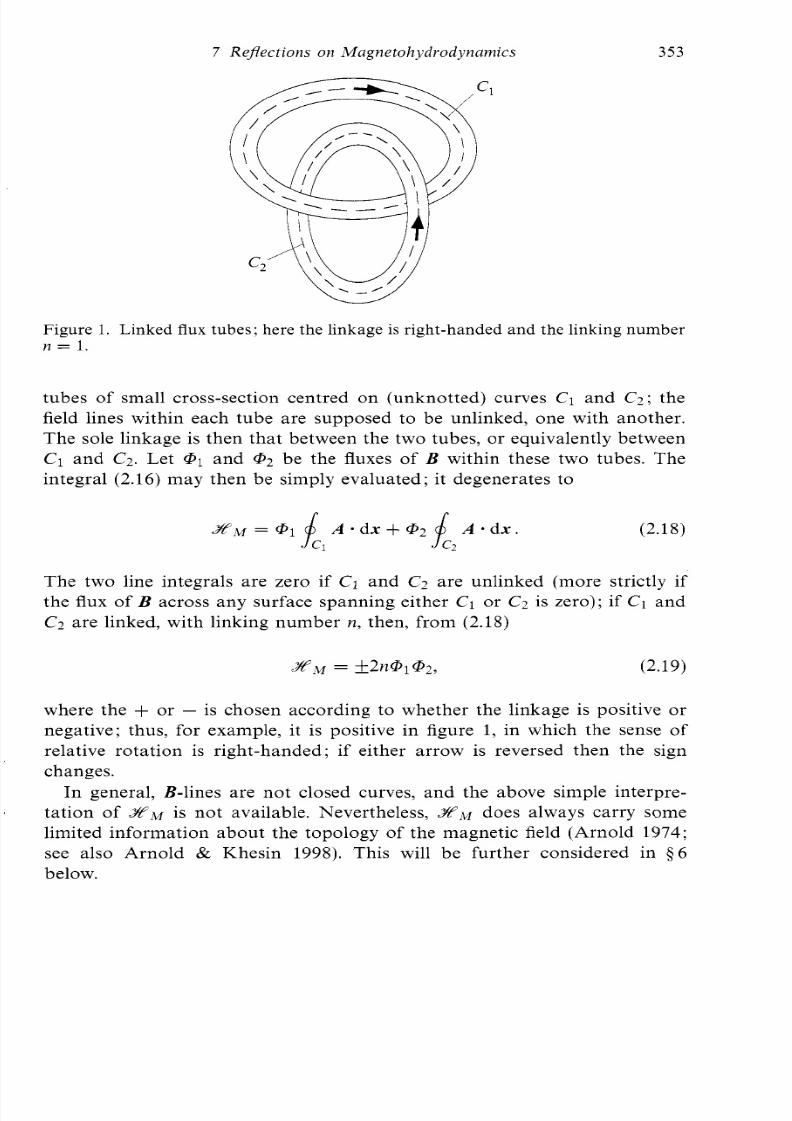
Figure 1. Linked flux tub es; here the linkage is right-handed and the linking numbern = 1.
tubes of small cross-section centred on (unknotted) curves C1 and C2; the
field lines within each tube are supposed to be unlinked, one with another.
The sole linkage is then that between the two tubes, or equivalently between
C1 and C2. Let @1 and @2 be the fluxes of B within these
integral (2.16) may then be simply evaluated ; it degenerates
two tubes. The
to
(2.18)
The two line integrals are zero if C1 and C2 are unlinked (more strictly if
the flux of B across any surface spanning either C1 or C2 is ze ro); if C1 and
C2 are linked, with linking num ber n, then, from (2.18)
(2.19)
where the + o r - s chosen according to whether the linkage is positive or
negative; thus, for example, it is positive in figure 1, in which the sense of
relative rotation is right-handed; if either arrow is reversed then the sign
changes.
In general, B-lines are not closed curves, and the above simple interpre-tation of S A w s not available. Nevertheless, X l w does always carry some
limited information about the topology of the magnetic field (Arnold 1974;
see also Arnold & Khesin 1998). This will be fu rthe r considered in $ 6
below.
t
8/3/2019 H.K. Moffatt- Reflections on Magnetohydrodynamics
http://slidepdf.com/reader/full/hk-moffatt-reflections-on-magnetohydrodynamics 8/45
354 H . K . MofSatt
3 The Lorentz force and the equation of motion
As indicated in the introduction, the Lorentz force in the fluid (per unit
volume) is F = j A B . With j = p;’V A B , this admits alternative expression
in terms of the Maxwell stress tensor
1 2
PO a x jF . ---- (B iB j - B2Sij) .
The first contribution, which may equally be written p ; ’ ( B * V ) B , epresents
a contribution to the force associated with curvature of B-lines directed
towards the centre of curvature; the second contribution, which may be
written -(2p0)-’VB2, represents (m inus) the gradient of ‘m agnetic pressure’
pLw= (2Po) - lB2 . (3.2)
In an incompressible fluid of constant density p, the equation of motion
including these contributions to the Lorentz force may be written in the
form
2 U 1- + v . V U = - V ~ + - B . V B + ~ V ~ ~ ,a t POP
(3.3)
where
x= ( P + PM / r> / P (3.4)
and v is the kinematic viscosity of the fluid. Coupled with the induction
equ ation (2.4) an d app ropriate bou ndary conditions, this determines the
evolution of the fields ( ~ ( x ,) ,B ( x , ) } .
We may illustrate this with reference to a phenomenon of central impor-
tance in M H D , namely the ability of the medium to su ppo rt transverse wave
motions in the presence of a mag netic field.
3.1 AlfvCn waves
Suppose that the medium is of infinite extent, and that we perturb about a
state of rest in which the fluid is permeated by a uniform magnetic field Bo.
Let U ( X , t ) and B = Bo +b ( x , ) be the perturb ed velocity an d m agnetic fields.
Then with the notation
v = ( p o p ) - 1 / 2 B o , h = ( ,~op ) -”~b , (3.5)
the linearized form s of equ ations (2.4) an d (3.3) (neglecting squares an dproducts of U and b ) are
(3.6)2v /Z t = -Vx + V * V h + v V ~ V ,
2h /d t = ( V * V ) U+ q V 2 h .
8/3/2019 H.K. Moffatt- Reflections on Magnetohydrodynamics
http://slidepdf.com/reader/full/hk-moffatt-reflections-on-magnetohydrodynamics 9/45
7 Re jec tion s on Magnetohydrodynamics 355
These equations admit wave-like solutions with = const. and
(3.7)(k*x-ur)
(U, h } e
provided
(-ice + v k 2 ) u = i(k * ~ ) h ,
(-im + q k 2 ) h= i(k - V ) U
Hence, for a non-trivial solution,
( i o - k2)(io- k 2 )= - ( k - v ) ~ ,
which is a quadratic equation for CO with roots
CO = - i i (q + v ) k 2 {4(k V ) 2- q- )”‘}li2 . (3.10)
In the ideal-fluid limit ( q = 0 , v = 0), the roots are real:
CO = f ( k * V ) , (3.11)
a dispersion relationship of rem arkab le simplicity. N ote th at the g roup
velocity associated with these waves is
c g = v k C O = f V , (3.12)
a result evidently independent of the wave-vector k . The associated non-
dispersive waves are kn ow n, after their discoverer, as Alfven waves, an d the
velocity V is the Alfven velocity (Alfven 1950).
When q + v # 0, these waves are invariably damped. In the liquid-metal
context, the damping is predominantly due to magnetic resistivity ( q >> v ) ;
if, moreover, the field Bo is strong in the sense tha t l k . Vl >> q2k4, then (3.8)
approximates to
CO rn - i i q k 2 + / i . V , (3.13)
If, on the other h and , l k . Vl << q 2 k 4 , hen the two roots (3.8) approxim ate
and the nature of the damping is clear.
to
CO x - iqk2, - i (k. v 1 2 / q k 2 . (3.14)
Now waves do not propagate, both modes are damped, and the first modeis damped much more rapidly than the second. Filtering of the first mode
from equations (3.6) may be achieved by simply dropping the term d h / ? t ;
in this approximation, the field perturbation h is instantaneously determined
by the flow U.
8/3/2019 H.K. Moffatt- Reflections on Magnetohydrodynamics
http://slidepdf.com/reader/full/hk-moffatt-reflections-on-magnetohydrodynamics 10/45
356 H. . Moffat t
4 Electromagnetic shaping and stirring
4.1 Two historic experiments
Two early papers provide examples of the manner in which applied mag-
netic fields and/or currents may contribute to the shaping of the regionoccupied by a conducting fluid and to the stirring of the fluid within this
region. The first is that of Northrup (1907) who described an experiment
in which a steady current is passed through a layer of conducting liquid
(sodium-potassium alloy N a K ) covered by a layer of (non-co ndu cting) oil.
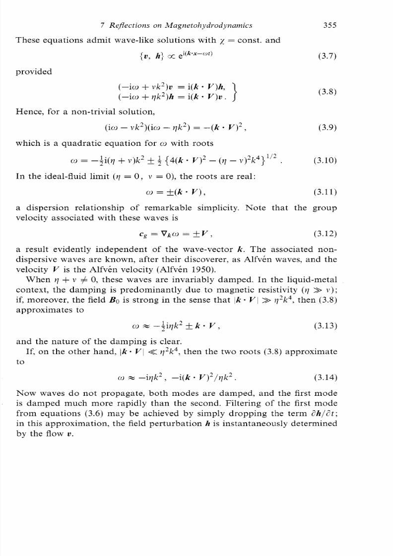
The configuration described by Northrup is shown, in plan and elevation,
in figure 2. The steady current j ( x ) passes through a constriction between
two electrodes on the boundary; the increased current density in this region
gives rise to an increased magnetic field encircling the current lines (viaAmpere’s Law); the resulting Lorentz force distribution causes depression
of the oil/NaK interface. Northrup attributes this observation to his friend
Car1 Hering who, he says, “jocosely called it the ‘pinch phenomenon’ ”. The
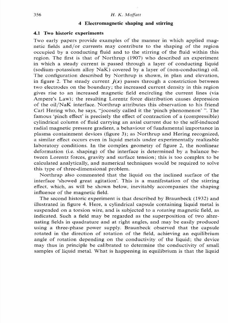
fam ous ‘pinch effect’ is precisely the effect of con traction of a (compressible)
cylindrical column of fluid carrying an axial current due to the self-induced
radial magnetic pressure gradient, a behaviou r of fundam ental importance in
plasma con tainme nt devices (figure 3); as Northrup and Hering recognized,
a similar effect occurs even in liquid metals under experimentally realizable
laboratory conditions. In the complex geometry of figure 2, the nonlinear
deform ation (i.e. shap ing) of the interface is determined by a balance be-
tween Lorentz forces, gravity and surface tension; this is too complex to be
calculated analytically, and numerical techniques would be required to solve
this type of three-dimensional problem.
Northrup also commented that the liquid on the inclined surface of the
interface ‘showed great agitation’. This is a manifestation of the stirring
effect, which, as will be shown below, inevitably accompanies the shaping
influence of the magnetic field.
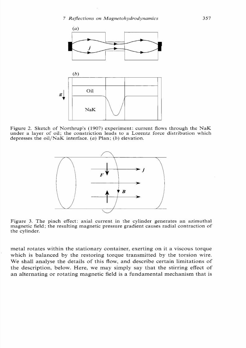
The second historic experiment is that described by Braunbeck (1932) an d
illustrated in figure 4. Here, a cylindrical capsule containing liquid metal is
suspended on a torsion wire, and is subjected to a rotating magnetic field, as
indicated. Such a field may be regarded as the superposition of two alter-
nating fields in quadrature and at right angles, and may be easily produced
using a three-phase power supply. Braunbeck observed that the capsulerotated in the direction of rotation of the field, achieving an equilibrium
angle of rotation depending on the conductivity of the liquid; the device
may thus in principle be calibrated to determine the conductivity of small
samples of liquid metal. What is happening in equilibrium is that the liquid
8/3/2019 H.K. Moffatt- Reflections on Magnetohydrodynamics
http://slidepdf.com/reader/full/hk-moffatt-reflections-on-magnetohydrodynamics 11/45
7 Reje ction s on Magnetohydrodynamics 351
.1
Oil
NaK
Figure 2. Sketch of Northrup’s (1907) experiment: current flows through the NaKunder a layer of oil; the constriction leads to a Lorentz force distribution whichdepresses the oil/NaK interface. (a) Plan; ( b ) elevation.
>
4
B
>
Figure 3. The pinch effect: axial current in the cylinder generates an azimuthalmagnetic field; the resulting magnetic pressure gradient causes radial contraction ofthe cylinder.
metal rotates within the stationary container, exerting on it a viscous torque
which is balanced by the restoring torque transmitted by the torsion wire.
We shall analyse the details of this flow, and describe certain limitations of
the description, below. Here, we may simply say that the stirring effect of
an alternating or rotating m agnetic field is a fundam ental mechanism that is
8/3/2019 H.K. Moffatt- Reflections on Magnetohydrodynamics
http://slidepdf.com/reader/full/hk-moffatt-reflections-on-magnetohydrodynamics 12/45
358 H . K . M o f a t t
Figure 4. Sketch of the experiment of Braunbeck (1932) a capsule, containing liquidmetal and suspended on a torsion wire, is subjected to a rotating magnetic field. Thisinduces rotation in the fluid; th e viscous torque o n the capsule is then in equilibriumwith th e torque transmitted by th e wire.
widely exploited in liquid-metal technology; thus, for example, it is used in
the continuous casting of steel to stir the melt before solidification in order
to produce a m ore h omogeneous end-prod uct (see, for example, Moffatt &
Proctor 1984).
4.2 Electrically induced stirring
N orthrup’s problem as described above is one of a general class of problems
in which a steady current distribution j ( x ) is established in the fluid ina domain 9 hrough prescription of an electrostatic potential distribution
cps(x) on the boundary S of this domain. This current, together with any
external current closing the circuit, is the source for the magnetic field
B ( x ) ,and flow is driven by the force F = j A B . If R, << 1, then additional
(indu ced) curren ts are weak, i.e. j ( x ) s effectively he same as if the con duc tor
were at rest. Hence j is determined through solution of a Dirichlet problem:
j=
-oVcp, (4.1)where
v2cp= O in 2 , cp = cpS(x) on S , (4.2)
and B ( x ) s then given by (2.1).
8/3/2019 H.K. Moffatt- Reflections on Magnetohydrodynamics
http://slidepdf.com/reader/full/hk-moffatt-reflections-on-magnetohydrodynamics 13/45
7 Reflections on Magnetohydrodynamics 359
8 = 0
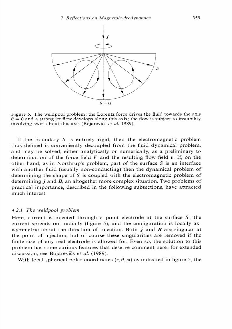
Figure 5. The weldpool problem: the Lorentz force drives the fluid towards the axis8 = 0 and a strong jet flow develops along this axis; the flow is subject to instabilityinvolving swirl about this axis (BojareviEs et al. 1989).
If the boundary S is entirely rigid, then the electromagnetic problemthus defined is conveniently decoupled from the fluid dynamical problem,
and may be solved, either analytically or numerically, as a preliminary to
determination of the force field F and the resulting flow field U. If, on the
other hand, as in Northrup’s problem, part of the surface S is an interface
with another fluid (usually non-conducting) then the dynamical problem of
determining the shape of S is coupled with the electromagnetic problem of
determining j and B , an altogether m ore com plex situation. Two problems of
practical importance, described in the following subsections, have attractedmuch interest.
4.2.1 Th e weldpool problem
Here, current is injected through a point electrode at the surface S ; the
current spreads out radially (figure 5 ) , and the configuration is locally ax-
isymmetric about the direction of injection. Both j and B are singular at
the point of injection, but of course these singularities are removed if the
finite size of any real electrode is allowed for. Even so, the solution to this
problem has some curious features th at deserve comm ent here; for extended
discussion, see BojareviEs et al. (1989).
With local spherical polar coordinates ( r ,8, c p ) as indicated in figure 5 , the
8/3/2019 H.K. Moffatt- Reflections on Magnetohydrodynamics
http://slidepdf.com/reader/full/hk-moffatt-reflections-on-magnetohydrodynamics 14/45
360 H . K . M offut t
current in the fluid is given by
and the corresponding field B is then given by,LQJin 6
2nr( 1+ cos 6)
Note the singularities at r = 0. The Lorentz force is given by
--p0J2 s in6 ,o) ,
F = j r \ B = 0,-( 47c2r3 1 + c os 6
(4.4)
(4.5)
This force, directed towards the axis 6 = 0, tends to drive the fluid towards
this axis; being incompressible, the fluid has no alternative but to flow out
along the axis in the form of a strong axisymm etric jet, which becomes
increasingly ‘focused’ for decreasing values of the fluid viscosity.
Experimental realization of this flow indicates a behaviour that is not
yet fully understood: the flow is subject to a strong symmetry-breaking
instability in which the fluid spontaneously rotates, in one direction or the
other, abo ut the axial direction 6 = 0. I t is believed that this rotation contro ls
the singularity of axial velocity that otherwise occurs if the dimensionlessparameter
K = p o J 2 / p ~ j 2 (4.6)
exceeds a critical va lue K , of order 300; a recent discussion of this perplexing
phenomenon is given by Davidson et al. (1999).
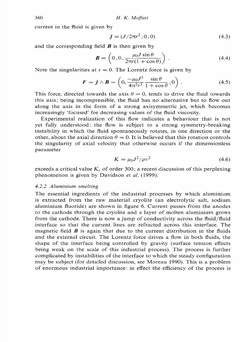
4.2.2 Aluminium smelting
The essential ingredients of the industrial processes by which aluminiumis extracted from the raw material cryolite (an electrolytic salt, sodium
aluminium fluoride) are shown in figure 6. Current passes from the anodes
to the cathode through the cryolite and a layer of molten aluminium grows
from the cathod e. The re is now a jum p of conductivity across the fluid/fluid
interface so that the current lines are refracted across this interface. The
magnetic field B is again that due to the current distribution in the fluids
and the external circuit. The Lorentz force drives a flow in both fluids, the
shape of the interface being controlled by gravity (surface tension effectsbeing weak on the scale of this industrial process). The process is further
com plicated by instabilities of the interface to which the s teady configuration
may be subject (for detailed discussion, see Moreau 1990). This is a problem
of enormous industrial importance: in effect the efficiency of the process is
8/3/2019 H.K. Moffatt- Reflections on Magnetohydrodynamics
http://slidepdf.com/reader/full/hk-moffatt-reflections-on-magnetohydrodynamics 15/45
7 Reflections on Magnetohydrodynamics 361
I 1 Anodes
v 1 / t f / f II I I
.pFathode
Figure 6. Sketch of the alum inium smelting process ( M ore au 1990). The interfacebetween the liquid cryolite and the molten aluminium is subject to instabilities ofmagnetohydrodynamic origin, which limit the efficiency of the process.
limited by instabilities that may lead to contact between the aluminium and
the anodes, a 'short-circuiting' that would terminate the process. This is a
billion-dollar industry for which an understanding of the fundamentals of
magnetohydrodynamics would appear to be a first essential.
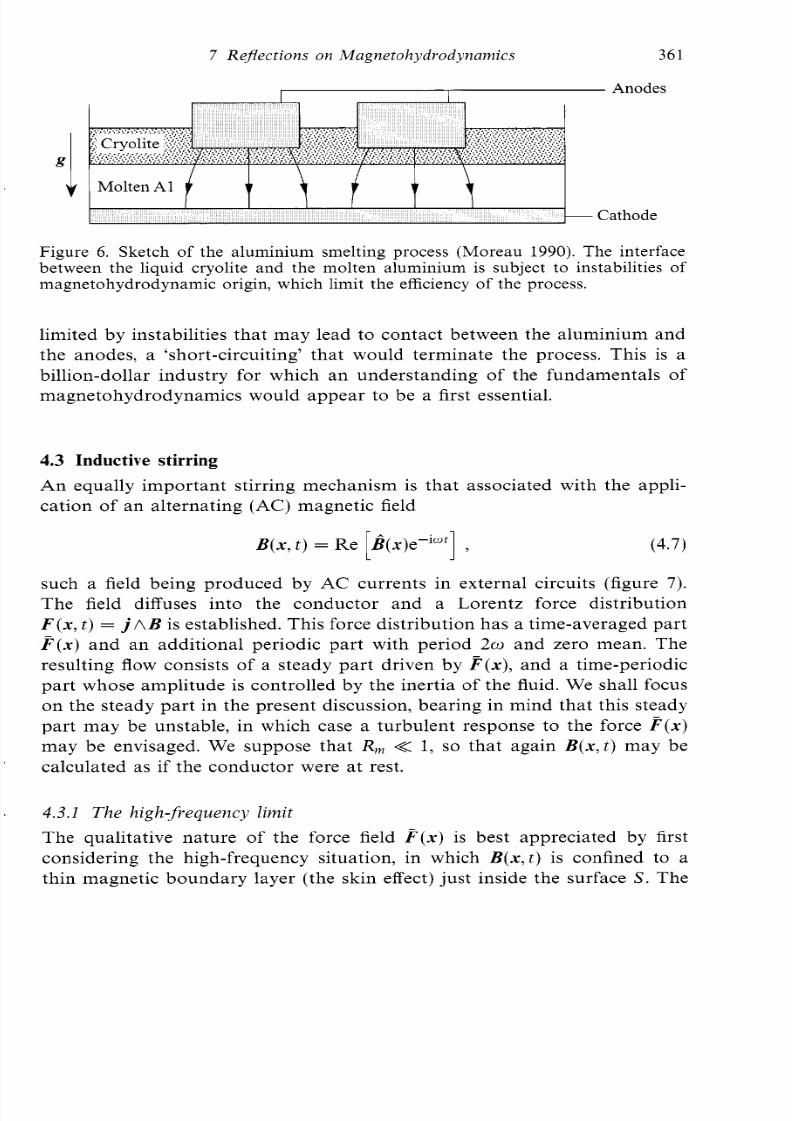
4.3 Inductive stirring
An equally important stirring mechanism is that associated with the appli-
cation of an alternating (AC) magnetic field
B ( x , t )= Re B(x)e-i"t ,[^ 1 (4.71
such a field being produced by AC currents in external circuits (figure 7).
The field diffuses into the conductor and a Lorentz force distribution
F ( x , ) = j A B is established. This force distribution has a time-averaged pa rt
P(x) and an additional periodic part with period 2co and zero mean. The
resulting flow consists of a steady part driven by P(x), and a time-periodic
part whose amplitude is controlled by the inertia of the fluid. We shall focus
on the steady part in the present discussion, bearing in mind that this steady
part may be unstable, in which case a turbulent response to the force P(x)
may be envisaged. We suppose that R, << 1, so that again B ( x , t ) may be
calculated as if the conductor were at rest.
4.3.1 The high-frequency limit
The qualitative nature of the force field P(x) is best appreciated by first
considering the high-frequency situation, in which B ( x , ) is confined to a
thin m agnetic bou nda ry layer (the skin effect) just inside the su rface S . The
8/3/2019 H.K. Moffatt- Reflections on Magnetohydrodynamics
http://slidepdf.com/reader/full/hk-moffatt-reflections-on-magnetohydrodynamics 16/45
362 H . K . Moftat t
C’
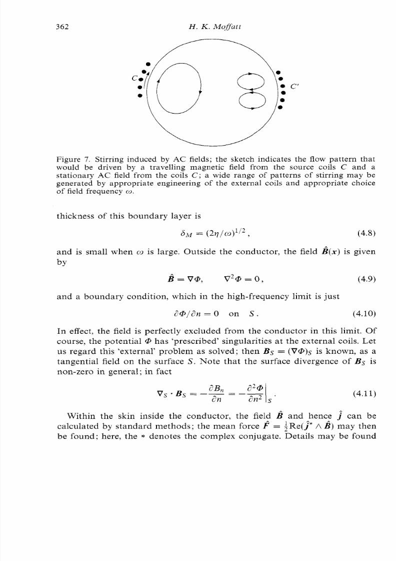
Figure 7. Stirring induced by AC fields; the sketch indicates the flow pattern thatwould be driven by a travelling magnetic field from the source coils C and astationary AC field from the coils C ; a wide range of patterns of stirring may begenerated by appropriate engineering of the external coils and appropriate choiceof field frequency U .
thickness of this boundary layer is
and is small when CO is large. Outside the conductor, the field &x) is given
by
B = V@, V2@= 0 , (4.9)
and a boundary condition, which in the high-frequency limit is just
2 @ / 2 n = O on S . (4.10)
In effect, the field is perfectly excluded from the conductor in this limit. Of
course, the potentia l @ has ‘prescribed’ singularities a t the externa l coils. Let
us regard this ‘external’ problem as solved ; then Bs = (V@)S is known, as a
tangential field on the surface S . Note that the surface divergence of Bs is
non-zero in general; in fact
(4.11)
Within the skin inside the conductor, the field B and hence j ^ can be
calculated by standard methods; the mean force f = ;Re(? A h) may then
be found; here, the * denotes the complex conjugate. Details may be found
8/3/2019 H.K. Moffatt- Reflections on Magnetohydrodynamics
http://slidepdf.com/reader/full/hk-moffatt-reflections-on-magnetohydrodynamics 17/45
7 Reflections on Magnetohydrodynamics 363
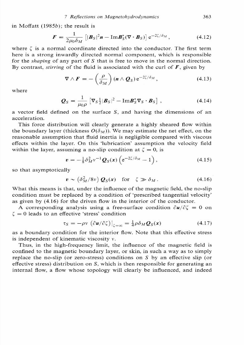
in M offatt (198521); the result is
(4.12)
where i s a normal coordinate directed into the conductor. The first termhere is a strong inwardly directed normal component, which is responsible
for the shaping of any part of S that is free to move in the normal direction.
By contrast, stirring of the fluid is associated with the curl of F , given by
(4.13)
where
(4.14)
a vector field defined on the surface S, and having the dimensions of an
acceleration.
This force distribution will clearly generate a highly sheared flow within
the boundary layer (thickness 0 ( 8 ~ ) ) .e may estim ate the net effect, on the
reasonable assumption that fluid inertia is negligible com pare d w ith viscous
effects within the layer. O n this ‘lubrication’ assum ption the velocity field
within the layer, assuming a no-slip condition at i= 0, is
so tha t asymptotically
(4.15)
(4.16)
W ha t this m eans is that, under the influence of the magnetic field, the no-slip
condition must be replaced by a condition of ‘prescribed tangential velocity’as given by (4.16) for the driven flow in the interior of the co ndu ctor.
A corresponding analysis using a free-surface condition 2u/2C: = 0 on
5 = 0 leads to an effective ‘stress’ condition
7s = PV ( 2 ~ l 2 i );== = $ P ~MQ~ ( . ) (4.17)
as a boundary condition for the interior flow. Note that this effective stress
is independent of kinematic viscosity v .
Thus, in the high-frequency limit, the influence of the magnetic field isconfined to the magnetic boundary layer, or skin, in such a way as to simply
replace the no-slip (or zero-stress) conditions on S by an effective slip (or
effective stress) dis tribu tion on S, which is then responsible for generating an
internal flow, a flow whose topology will clearly be influenced, and indeed
8/3/2019 H.K. Moffatt- Reflections on Magnetohydrodynamics
http://slidepdf.com/reader/full/hk-moffatt-reflections-on-magnetohydrodynamics 18/45
364 H . K . Moflatt
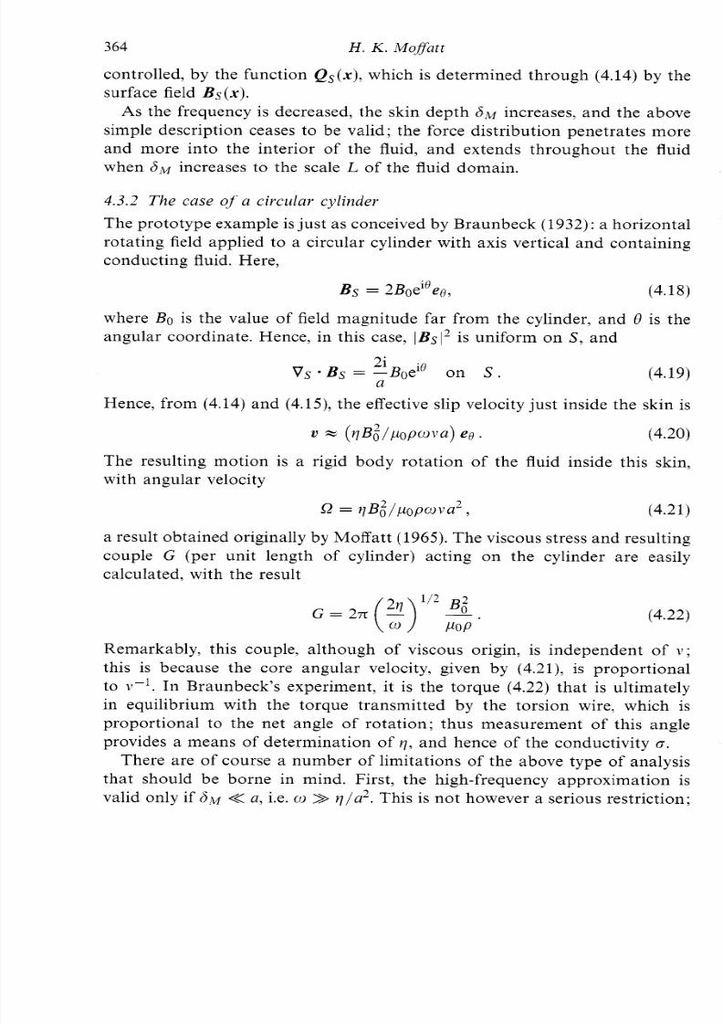
controlled, by the function Qs(x) , which is determined through (4.14) by the
surface field B s ( x ) .
As the frequency is decreased, the skin depth JLw ncreases, and the above
simple description ceases to be valid; the force distribution penetrates more
and more into the interior of the fluid, and extends throughout the fluidwhen 8-v increases to the scale L of the fluid domain.
4.3.2 Th e case of a circular cylinder
The prototype example is just as conceived by Braunbeck (193 2): a ho rizontal
rotating field applied to a circular cylinder with axis vertical and containing
conducting fluid. Here,
Bs = 2Boeieee, (4.18)
where Bo is the value of field magnitude far from the cylinder, and 0 is the
angular coordinate. H ence, in this case, IBs12 is uniform on S , and
2iVs Bs = -Boeie on S
U(4.19)
Hence, from (4.14) and (4.15), the effective slip velocity jus t inside the skin is
21 = (11B;iPofwva) e e . (4.20)
The resulting motion is a rigid body rotation of the fluid inside this skin,
with angular velocity
SZ = YBi/popova2, (4.21)
a result obtained originally by Moffatt (1965). Th e viscous stress and resu lting
couple G (per unit length of cylinder) acting on the cylinder are easily
calculated, with the resultB i
G = 2 r r ( ? ) - .POP
(4.22)
Remarkably, this couple, although of viscous origin, is independent of v ;
this is because the core ang ular velocity, given by (4.21), is pro po rtional
to v l . n Braunbeck’s experiment, it is the torque (4.22) that is ultimately
in equilibrium with the torque transmitted by the torsion wire, which is
proportional to the net angle of rotation; thus measurement of this angleprovides a means of determination of 11, and hence of the conductivity g.
There are of course a number of limitations of the above type of analysis
that should be borne in mind. First, the high-frequency approximation is
valid only if 6.v << a, i.e. cc) >> q / a 2 . This is not however a serious restriction;
8/3/2019 H.K. Moffatt- Reflections on Magnetohydrodynamics
http://slidepdf.com/reader/full/hk-moffatt-reflections-on-magnetohydrodynamics 19/45
7 Re$ections on Magne tohydvody namics 365
the problem can be solved exactly for arbitrary CO in term s of Bessel func tions.
More seriously however, the analysis fails if the field strength Bo becomes
so strong that Q in (4.21) becomes comparable with C O ; for it is in fact not
the absolute angular velocity w of the field that is relevant to the induction
of currents, bu t rather the relative angular velocity w -Q between field andfluid. This strong field situation requires a major modification of approach
(see, for example, M oreau 1990, where prob lems of this type are extensively
treated).
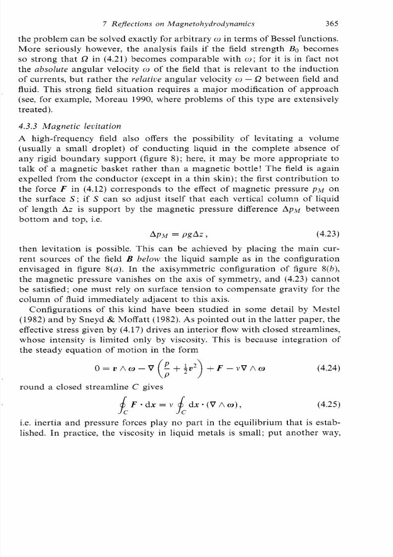
4.3.3 Magnetic lecitation
A high-frequency field also offers the possibility of levitating a volume
(usually a small droplet) of conducting liquid in the complete absence of
any rigid boundary support (figure 8); here, it may be more appropriate totalk of a magnetic basket rather than a magnetic bottle! The field is again
expelled from the conductor (except in a thin skin); the first contribution to
the force F in (4.12) corresponds to the effect of magnetic pressure p . ~n
the surface S ; if S can so adjust itself that each vertical column of liquid
of length A z is support by the magnetic pressure difference Ap-w between
bottom and top, i .e.
APM = PgAz , (4.23)then levitation is possible. This can be achieved by placing the main cur-
rent sources of the field B below the liquid sample as in the configuration
envisaged in figure 8(a) . In the axisymmetric configuration of figure 8( b ) ,
the magnetic pressure vanishes on the axis of symmetry, and (4.23) cannot
be satisfied; one must rely on surface tension to compensate gravity for the
column of fluid immediately adjacent to this axis.
Configurations of this kind have been studied in some detail by Mestel
(1982) an d by Sneyd & M offatt (1982).As pointed out in the latter pap er, the
effective stress given by (4.17) drives an inte rior flow with closed streamlines,
whose intensity is limited only by viscosity. This is because integration of
the steady equation of motion in the form
O = V A C O - V - + - U + F - v V A C O (4.24)(; ?>
round a closed streamline C gives
(4.25)
i.e. inertia and pressure forces play no part in the equilibrium that is estab-
lished. In practice, the viscosity in liquid metals is small; put another way,
8/3/2019 H.K. Moffatt- Reflections on Magnetohydrodynamics
http://slidepdf.com/reader/full/hk-moffatt-reflections-on-magnetohydrodynamics 20/45
366
( a )
H . K . MofSatt
Axis ofsymmetry
Levitated molten
current
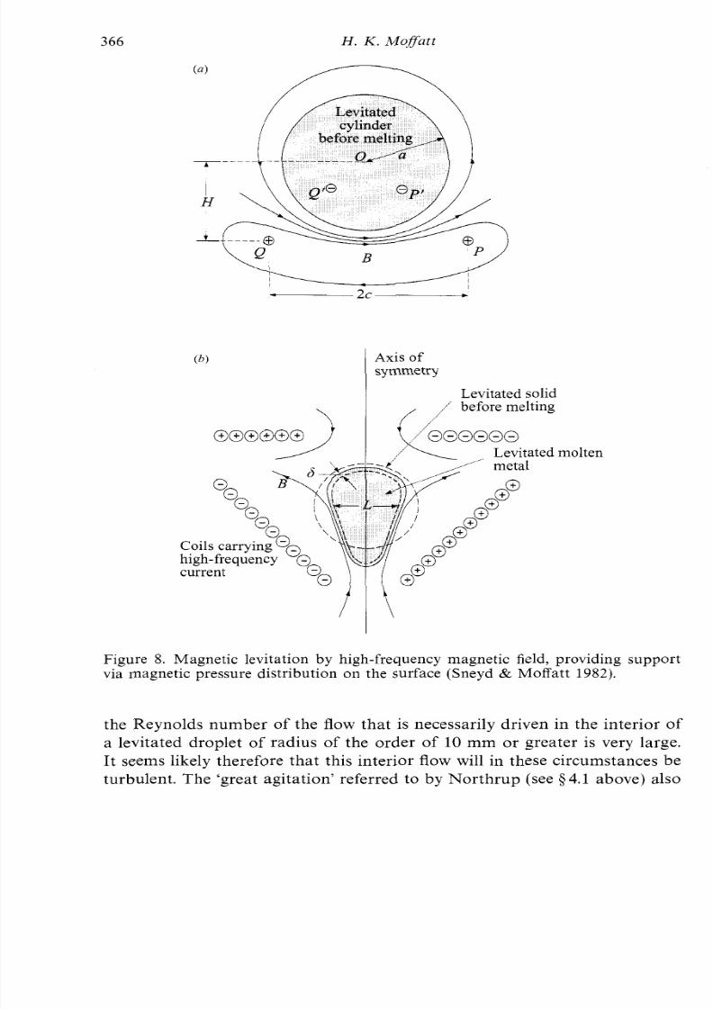
Figure 8. Magnetic levitation by high-frequency magnetic field, providing supportvia magnetic pressure distribution on the surface (Sneyd & Moffatt 1982).
the Reynolds number of the flow that is necessarily driven in the interior of
a levitated droplet of radius of the order of 10 mm or greater is very large.
It seems likely therefore tha t this interio r flow will in these circum stances be
turbulen t. The ‘great agitation’ referred to by N or thr up (see $4 .1 above) also
8/3/2019 H.K. Moffatt- Reflections on Magnetohydrodynamics
http://slidepdf.com/reader/full/hk-moffatt-reflections-on-magnetohydrodynamics 21/45
7 Reflections on Magnetohydrodynamics 367
presumably indicated a state of turbulent flow just inside the liquid metal -and for similar reasons.
5 Dynamo theoryDynamo theory is concerned with explaining the origin of magnetic fields
in stars, planets and galaxies. Such fields are produced by currents in the
interior regions, which would in the normal course of events be subject to
ohm ic decay, in the same way tha t curre nt in a n electric circuit decays if not
maintained by a battery. This decay can however be arrested, and indeed
reversed, through inductive effects associated with fluid motion; when this
happen s, the fluid system acts as a self-exciting dynam o. Th e m agnetic field
grows spontaneously from an arbitrary weak initial level, in much the sameway as any other perturbation of an intrinsically unstable situation.
The possibility of such ‘dynamo’ instabilities may be understood with
reference to the induction equation (2.4), which governs field evolution if
the velocity field v ( x , t ) in the fluid is regarded as ‘given’. Let us suppose
for simplicity that the fluid fills all space, and that the velocity field is
steady, i.e. U = u ( x ) . We must suppose also that B has no ‘sources at
infinity’ which would m itigate against the concep t of an internally gen erated
dynamo.
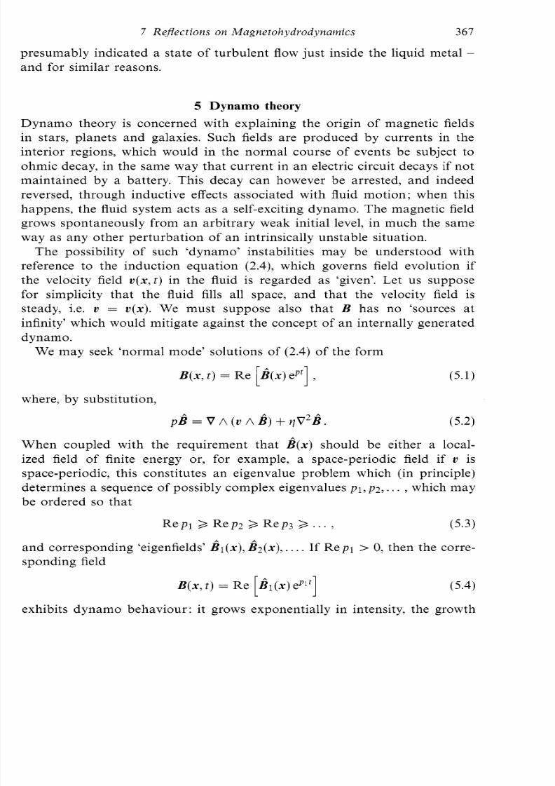
We may seek ‘normal mode’ solutions of (2.4) of the form
where, by substitution,
pB = v A ( U A B ) + y v 2 B . (5 .2 )
When coupled with the requirement that &x) should be either a local-ized field of finite energy or, for example, a space-periodic field if U is
space-periodic, this constitutes an eigenvalue problem which (in principle)
determ ines a sequence of possibly complex eigenvalues p1, p2,. . . ,which may
be ordered so that
R e p l 3 Rep2 3 Rep3 3 . . . , (5 .3)
an d correspond ing ‘eigenfields’B~(x),(x) , . . . I f Repl > 0, then the corre-
sponding field
B ( x , ) = Re [ B ~ ( x )Plf] (5.4)
exhibits dynamo behaviour: it grows exponentially in intensity, the growth
8/3/2019 H.K. Moffatt- Reflections on Magnetohydrodynamics
http://slidepdf.com/reader/full/hk-moffatt-reflections-on-magnetohydrodynamics 22/45
368 H . K . M o f a t t
being oscillatory or non-oscillatory according to whether Imp1 # 0 or = 0.
The mode of maximum growth-rate is clearly the one that will emerge from
an arbitrary initial condition in which all modes may be present.
If this exponential growth occurs, then it can persist only for as long as
the velocity field u ( x ) remains unaffected by the Lorentz force. This is the‘kinematic phase’ of the dynamo process. Obviously, however, the Lorentz
force increases exponentially with growth rate 2Re p 1 (considering only the
mode (5.4)) and so ultimately the back-reaction of the Lorentz force on
the fluid motion must be take n into acc oun t. This is the ‘dynamic phase’ of
dyn am o action in which the nature of the supply of energy to the system (via
the dynamic equation of motion) must be considered. While great progress
has been made over the past 50 years towards a full understanding of th e
kinematic phase, the highly nonlinear dynamic phase has proved far moreintractable from an analytical point of view, and is likely to remain a focus
of much research effort, both computational and analytical, over the next
few decades.
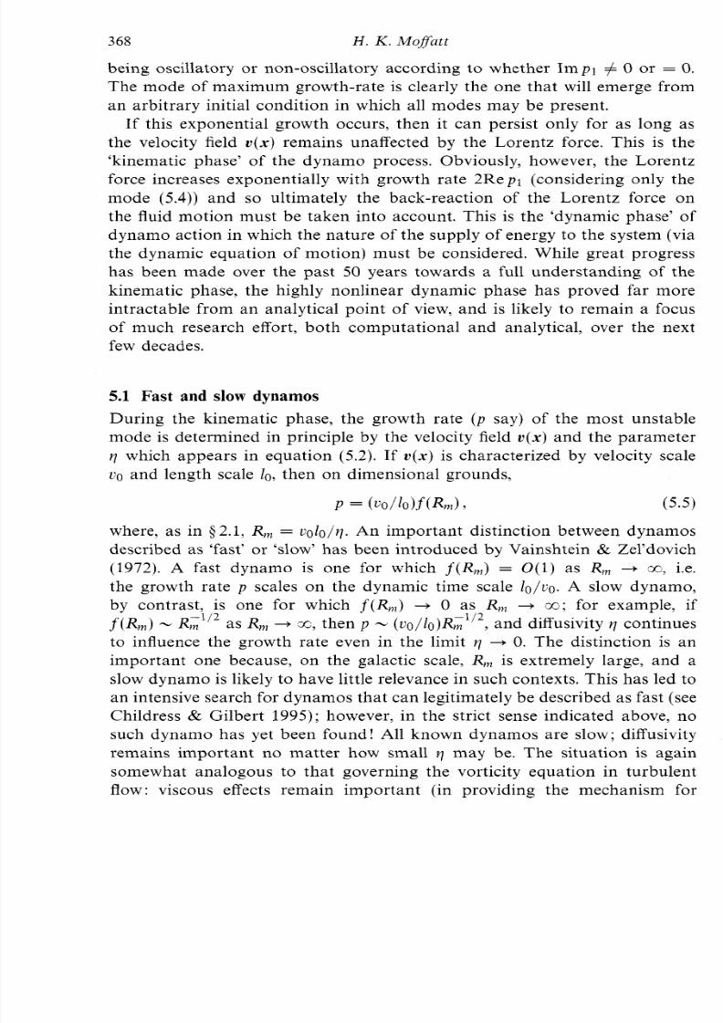
5.1 Fast and slow dynamos
During the kinematic phase, the growth rate ( p say) of the most unstable
mode is determined in principle by the velocity field u ( x ) and the parametery which appe ars in equation (5.2). If u ( x ) is characterized by velocity scale
uo and length scale lo , then on dimensional grounds,
where, as in $2.1, R, = t ’olo/y. An important distinction between dynamos
described as ‘fast’ or ‘slow’ ha s been introduced by V ainshtein & Zel’dovich
(1972). A fast dyna m o is one fo r which f ( R m )= 0 ( 1 ) as R, -+ x, .e.
the growth rate p scales on the dynamic time scale l o / v o . A slow dynamo,by contrast, is one for which f(R,) + 0 as R, -+ E; for example, if
f(R,) - R,1’2 as R, -+ x,hen p - co/ l~)R~’” ,nd diffusivity y continues
to influence the growth rate even in the limit y + 0. The distinction is an
important one because, on the galactic scale, R, is extremely large, and a
slow dynam o is likely to have little relevance in such con texts. Th is has led to
an intensive search for dynam os th at can legitimately be described as fast (see
Childress & Gilbert 199 5); however, in the strict sense indicated above, no
such dynamo has yet been found! All known dynamos are slow; diffusivity
remains important no matter how small y may be. The situation is again
somewhat analogous to that governing the vorticity equation in turbulent
flow: viscous effects remain important (in providing the mechanism for
8/3/2019 H.K. Moffatt- Reflections on Magnetohydrodynamics
http://slidepdf.com/reader/full/hk-moffatt-reflections-on-magnetohydrodynamics 23/45
7 Reflections on Magnetohydrodynamics 369
dissipation of kinetic energy) no matter how small the kinematic viscosity 1’
may be.
When a dynamo enters the dynamic phase (assuming that sufficient time
is available for it to do so) the distinction between fast and slow behaviour
disappears; in either case, the growth rate must decrease, ultimately to zero
when an equilibrium between generation of magnetic field by the (modified)
velocity field and ohmic dissipation of magnetic field is established.
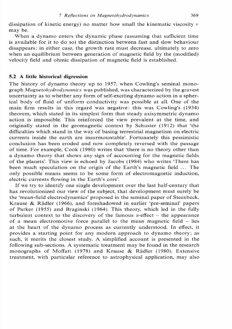
5.2 A little historical digression
The history of d yn am o theory u p to 1957, when Cowling’s seminal mono -
graph Magnetohydrodynamics was pub lished, was characterized by the gravest
uncertainty as to whether an y form of self-exciting dy na m o action in a spher-
ical body of fluid of uniform conductivity was possible at all. One of the
main firm results in this regard was negative: this was Cowling’s (1934)
theorem, which stated in its simplest form that steady axisymmetric dynamo
action is impossible. This reinforced the view prevalent at the time, and
originally stated in the geomagnetic context by Schuster (1912) that ‘the
difficulties which stand in the way of basing terrestrial magnetism on electric
currents inside the earth are insurmountable’. Fortunately this pessimisticconclusion has been eroded and now completely reversed with the passage
of time. For example, Cook (1980) writes that ‘there is no theory other than
a dynamo theory that shows any sign of accounting for the magnetic fields
of the planets’. This view is echoed by Jacobs (1984) who writes ‘There has
been much speculation on the origin of the Earth’s magnetic field . . . The
only possible means seems to be some form of electromagnetic induction,
electric currents flowing in the Earth’s core’.
If we try to identify one single development over the last half-century thathas revolutionized ou r view of the sub ject, that developm ent must surely be
the ‘mean-field electrodynamics’ proposed in the seminal paper of Steenbeck,
Krause & Ra dler (1966), and foreshadow ed in earlier ‘pre-seminal’ pap ers
of Parker (1955) an d Braginski (1964). This theory , which led in the fully
turbulent context to the discovery of the famous x-effect - the appearance
of a mean electromotive force parallel to the mean magnetic field - lies
at the heart of the dynamo process as currently understood. In effect, it
provides a starting point for any modern approach to dynamo theory; assuch, it merits the closest study. A simplified account is presented in the
following sub-sections. A systematic treatm ent may be found in the research
monographs of Moffatt (1978) and Krause & Radler (1980). Extensive
treatment, with particular reference to astrophysical application, may also
’
8/3/2019 H.K. Moffatt- Reflections on Magnetohydrodynamics
http://slidepdf.com/reader/full/hk-moffatt-reflections-on-magnetohydrodynamics 24/45
370 H . K . MofSatt
be found in the boo ks of Parker (1979) an d Zeldovich, Ruzm aikin & Sokoloff
(1983).
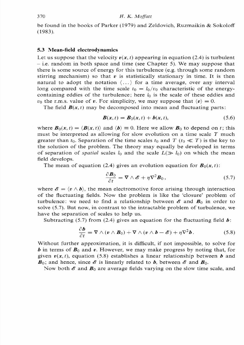
5.3 Mean-field electrodynamics
Let us suppose that the velocity U ( X , t ) app earing in equa tion (2.4) is turbu lent- i.e. random in both space and time (see Chapter 5 ) . We may suppose that
there is some sou rce of energy for this turbulence (e.g. throu gh some ra nd om
stirring mechanism) so that v is statistically stationary in time. It is then
natural to adopt the notation ( . . ) for a time average, over any interval
long compared with the time scale to = l o / t ' o characteristic of the energy-
containing eddies of the turbulence; here lo is the scale of these eddies and
00 the r.m.s. value of v . For simplicity, we m ay sup pose th at ( U ) = 0.
The field B ( x , ) may be decomposed into mean and fluctuating parts:
B ( x , )= Bo(x , ) + b ( x , ) , (5 .6)
where Bo(x , ) = ( B ( x , ) ) and ( 6 ) 0. Here we allow Bo to depend on t ; his
must be interpreted as allowing for slow evolution on a time scale T much
greater tha n to. Separation of the time scales to and T ( to << T ) s the key to
the solution of the problem. The theory may equally be developed in termsof separation of spatial scales 20 and the scale L(>> o ) on which the mean
field develops.
The mean of equation (2.4) gives an evolution equation for Bo(x , ) :
where 8 = ( U A b ) , the mean electromotive force arising through interaction
of the fluctuating fields. Now the problem is like the 'closure' problem ofturbulence: we need to find a relationship between B and Bo in order to
solve (5.7). But now, in contrast t o the intractable problem of turbulence, we
have the separation of scales to help us.
Subtracting (5.7) from (2.4) gives an e qua tion for the fluctuating field b :
o'b
2 t= v A ( U ABo)t V ( U A b -8) qV2b
Without further approximation, it is difficult, if not impossible, to solve forb in terms of Bo and v . However, we may make progress by noting that, for
given U ( X , t j , equation (5 .8 ) establishes a linear relationship between b and
Bo; an d hence, since Q is linearly related to b, between Q and Bo.
Now both Q and Bo are average fields varying on the slow time scale, and
8/3/2019 H.K. Moffatt- Reflections on Magnetohydrodynamics
http://slidepdf.com/reader/full/hk-moffatt-reflections-on-magnetohydrodynamics 25/45
7 Re jec tio ns on Magnetohydrodynamics 371
on the large length scale L ; hence this linear relationship between € and Bo
may be represented by a series of the form
where x i j , P i j k , . . . are tensor (actually p seud o-tensor) coefficients which a re in
principle determined by the statistical properties of the turbulent field U(X, )
and the parameter q which intervenes in the solution of (5.8). Note that
successive terms of (5.9) decrease in magnitude by a factor of order lo/L;
an d tha t any terms involving time derivatives, i.e. dBo/dt , may be eliminated
in favou r of space derivatives throu gh recursive app eal to equa tion (5.7).That
the coefficients r i j , P i j k , . . . are pseudo-tensors (rather than tensors) should
be evident from the fact that € is a polar vector (like velocity) whereas Bois an axial vector (like angular velocity).
We may go further on the simplifying assumption that the turbulence is
homogeneous and isotropic. In this case, X i j and P i j k share these properties,
i.e. they are isotropic pseudo-tensors invariant under translation, i.e. inde-
pendent of x (they are already ind epende nt of t from the assumption that U
is statistically station ary). Isotropy is a very strong co ns train t; it implies tha t
(5.10)
where now x is a pseudo-scalar quantity and P is a pure scalar. Hence (5.9)
simplifies to
€ = aBo - ( V A Bo)+ . ; (5.11)
the next term in this series involves V A (V A Bo) and so on. This is th e
required relationship between € and Bo.
Substituting this back into (5 .7)gives the mean-field equation in its simplestform : - 0 A Bo)+ ( q + P)V2B0+ .dB0
2 t(5.12)
where the terms indicated by + . involve higher derivatives of Bo, and may
presum ably be neglected when the scale of variation of Bo is large. I t is clear
from the structure of (5.12) that P must be interpreted as an 'eddy diffusivity'
associated with the turbulence (althoug h there is no guarantee from the above
treatment tha t P mu st invariably be positive!). The first term on the right of(5.12) will however always do m inate the evolution, provided x f 0 and the
scale of Bo is sufficiently large. Before going further it is therefore essential
to find a means of calculating 3 explicitly and determining the conditions
under which this key parameter is definitely non-zero.
8/3/2019 H.K. Moffatt- Reflections on Magnetohydrodynamics
http://slidepdf.com/reader/full/hk-moffatt-reflections-on-magnetohydrodynamics 26/45
372 H . K . MofSatt
5.4 First-order smoothing
To do this, it is legitimate to consider the situation in which Bo is constant;
the reason for this is that tl is independent of the field B o ( x , t ) , and we
are free to m ake any assum ption abou t this field tha t simplifies calculation
of a. The assumption that Bo is constant is equivalent to considering the
conceptual limit L + sc, T + sc.
Under this condition, the fluctuation equation (5.8) becomes
(5.13)‘b- = (Bo V)U+ V A ( v A b -8) yV2b.2 t
Now we know that, if the magnetic Reynolds number R, = v o l ~ / y s small,
then the induced field b is weak compared with Bo (actually b = O(R,)Bo;
see below). In this circumstance, the awkward term V A ( U A b - €) in (5.8)
is negligible compared with the other terms in the equation and may be
neglected. We then have a linear equation with constant coefficients which
may be solved by elementary Fourier techniques. Let us then make this
assumption and explore the consequences.
It is illuminating to consider first the situation in which v is a circularly
polarized wave of the form
~ ( x ,) = vo(sin(kz- ot),cos(kz - ot),0 ) , (5.14)
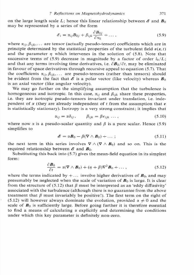
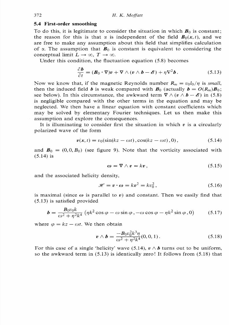
and Bo = (O,O, Bo) (see figure 9). Note that the vorticity associated with
(5.14) is
w = V A v = k v , (5.15)
and the associated helicity density,
is maximal (since w is parallel to U ) and constant. Then we easily find that
(5.13) is satisfied provided
where cp = kz - at. We then obtain
(5.18)
Fo r this case of a single ‘helicity’ wave (5.14), v A b turns out to be uniform,
so the awkward term in (5.13) is identically z ero! It follows from (5.18) tha t
8/3/2019 H.K. Moffatt- Reflections on Magnetohydrodynamics
http://slidepdf.com/reader/full/hk-moffatt-reflections-on-magnetohydrodynamics 27/45
7 Reflections on Magnetohydrodynamics 373
Z
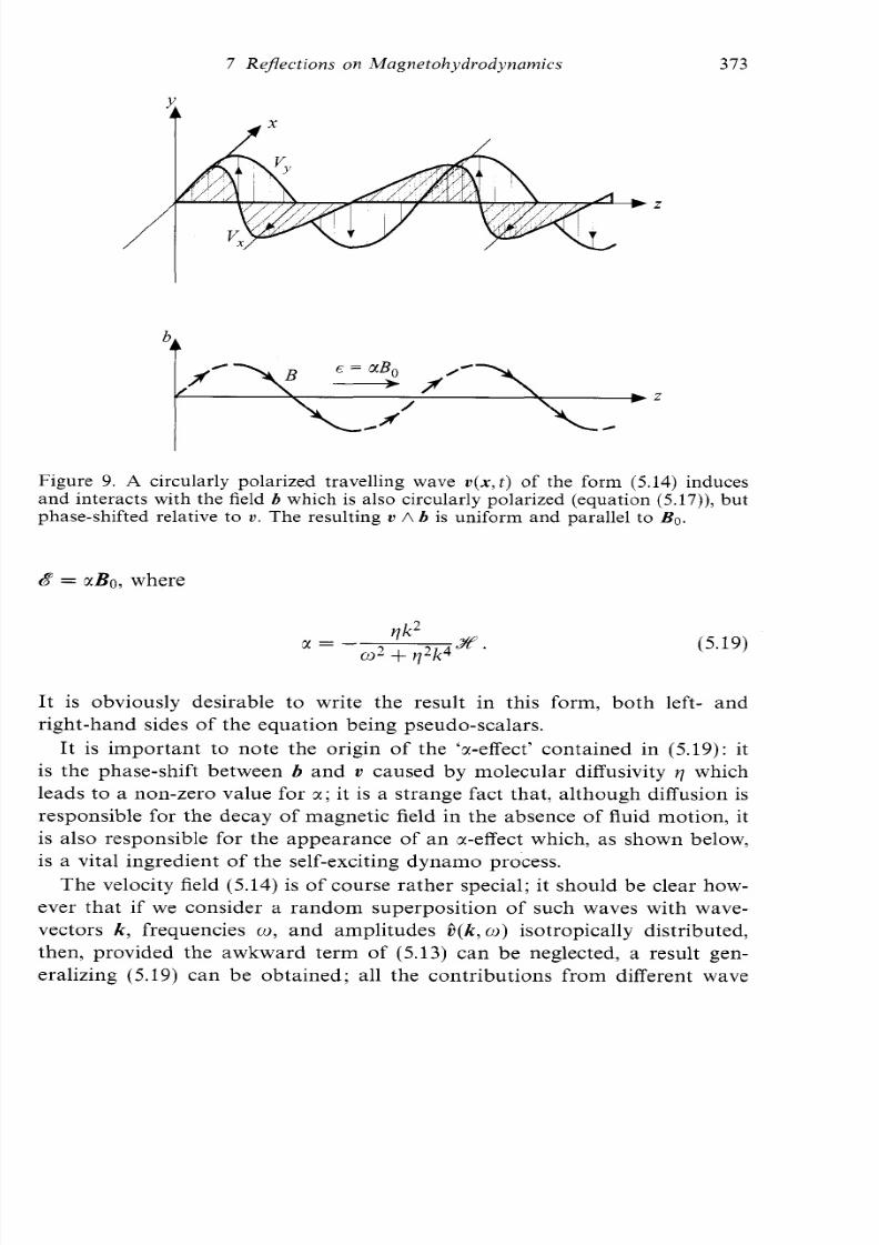
Figure 9. A circularly polarized travelling wave v ( x , t ) of the form (5.14) inducesand interacts with the field b which is also circularly polarized (equation (5.17)),butphase-shifted relative to v . The resulting U A b is uniform and parallel to Bo.
B = rBo, where
(5.19)
It is obviously desirable to write the result in this form, both left- andright-hand sides of the equation being pseudo-scalars.
It is important to no te the origin of the ‘r-effect’ conta ined in (5.19): it
is the phase-shift between b and v caused by molecular diffusivity y which
leads to a non-zero value for r ; t is a strange fact tha t, althou gh diffusion is
responsible for the decay of magnetic field in the absence of fluid motion, it
is also responsible for the appearance of an &-effectwhich, as shown below,
is a vital ingredient of the self-exciting dynamo process.
Th e velocity field (5.14) is of course rather special; it should be clear how-ever that if we consider a random superposition of such waves with wave-
vectors k, frequencies CO , and amplitudes 6 ( k , O) isotropically distributed,
then, provided the awkward term of (5.13) can be neglected, a result gen-
eralizing (5.19) can be obtained; all the contributions from different wave
8/3/2019 H.K. Moffatt- Reflections on Magnetohydrodynamics
http://slidepdf.com/reader/full/hk-moffatt-reflections-on-magnetohydrodynamics 28/45
374 H . K . M o f a t t
modes are additive, and the final result is
(5.20)
where X(k,co) is the helicity spectrum function of the velocity field U, withthe property
( U - a)=/I(k , co)d3k dco . (5.21)
The factor 3 appears in (5.20) from averaging over all directions. The main
thing to note again is the direct relationship between x and the helicity of
the turbulent field.
This theory, usually described as ‘first-order smoothing’ theory, is limited
to circumstances in which, as indicated above, lbl << IBol. This condition is
satisfied if R, << 1; it is also satisfied under the alternative condition
k2%(k, 03) d 3 kd oa = - : q / J c o 2 + Y 2 k 4 ,
Ivok/ol << 1 (5.22)
for values of k and co making the dominant contributions to the field of
turbulence. The condition (5 .22) is relevant in a rap idly rota ting system in
which the turbulence is more akin to a field of weakly interacting inertialwaves whose frequencies co are of the order of the angular velocity fi of the
system; in this context, the condition (5.22) is one of small Rossby number.
If neither of the above conditions is satisfied, then it is not legitimate to
neglect the awk ward term in (5.13 ); no fully satisfactory theory is as yet
available for the determination of a in these circumstances. Nevertheless,
one may assert that the key property of turbulence required to provide a
non-zero value for a is that its statistical properties should lack reflectional
symmetry, i .e. should be non -invariant under change from a right-hand ed toa left-handed frame of reference; it is this same property that is necessary
to provide non-zero mean helicity J? = (U - U), hich is indeed a simple
measure of ‘lack of reflectional sym metry’, an d so a loose connex ion between
x and .At s to be expected.
The concept of isotropic turbulence that lacks reflectional symmetry is
quite novel! O ne o ften think s of a turbu lent vorticity field in pictorial terms
as like a ran do m field of spag hetti; to picture turbulence lacking reflectional
symmetry, think rather of a pasta in which each pasta element is twistedwith the same sense of twist - say right-handed: if the vorticity field follows
the sense of these elements, it remains statistically isotropic but acquires
positive helicity. For a more realistic example, it suffices to consider Benard
convection in a rotating system (see, for exam ple, Ch an dra sek ha r 1961 ); it
8/3/2019 H.K. Moffatt- Reflections on Magnetohydrodynamics
http://slidepdf.com/reader/full/hk-moffatt-reflections-on-magnetohydrodynamics 29/45
7 Re jec tion s on Magnetohydrodynamics 375
turns out that the average of v w over horizontal planes is non-zero and
antisymm etric abou t the centreplane (M offatt 1978, chap . 10).
5.5 Dynamo action associated with the x-effect
Let us retur n now to the m ean field equation (5.12) in the form
(5.23)
where now y e = y + p is the ‘effective diffusivity’, an d we d ro p the suffix 0 on
Bo, to simplify notation. The simplest way to treat (5.23) is to seek solutions
which have the Beltrami property
V A B =K B , (5 .24)
where K is a co nstant. F or example, the field
B = (c sin K z + b cos Ky , a sin K x + c cos Kz , b sin K y + a c o s K x ) (5.25)
(th e ‘abc’ field) has this pro perty, as m ay be easily verified. We shall suppose
that K is chosen to have the same sign as x, i.e. xK > 0, and that IKI is
small, so that the scale L
-K-’ of B is large com pared with the scale lo
of the underlying turbulence that gives rise to the x-effect. Of course (5.23)
implies tha t
(5.26)B = -V A ( V A B ) = - K ~ B ,
and so (5.23) becomes
(5.27)
so that
B(x, t ) = B(x, 0) ePt , (5.28)
where
P = a K - V e K 2 . ( 5 . 2 9 )
Obviously we have exponential growth of the mean field B provided
aK > ye K 2, .e. provided
IKI < laI/Ye. (5.30)
Thu s we have a d yn am o effect, in w hich the m ean field (i.e. the field on the
large scale L ) grows exponentially provided L is large enough.
8/3/2019 H.K. Moffatt- Reflections on Magnetohydrodynamics
http://slidepdf.com/reader/full/hk-moffatt-reflections-on-magnetohydrodynamics 30/45
376 H . K . Moffat t
If we adopt the low-Rm estimate for x (based on (5.20)),
(5.31)
assuming 2 -i / l o , and note that in this lOw-Rm situation, p << q (actually
/3 = O (R i) q ), then the scale of maximum growth rate is given (from (5.29))
L - K-‘ - RG210. (5.32)
Hence a new magnetic Reynolds number Am defined in terms of L rather
than 10 is given by
by
- Luo 2Rm=
- R i Rm
-R i l .
Y(5.33)
The condition Rm << 1 implies that R m >> 1: the field grows on a scale L a t
which the corresponding R m is large.
We can now summarize the implications of the above discussion. If a
conducting fluid is in turbulent motion, the turbulence being homogeneous
and isotropic but having the crucial property of ‘lack of reflectional symm e-
try’ (a property that, as observed above, can be induced in a rotating fluid
through interaction of buoyancy-induced convection and Coriolis forces),
then a magnetic field will in general grow from an arbitrarily weak initial
level, on a scale L large compared with the scale 10 of the turbulence. This is
one of these remarkable situations in which ‘order arises out of chaos’, the
order being evident in the large-scale magnetic field. It may be appropriate
to follow the example of Richardson (1922) by summarizing the situation in
rhyme :
Conuection and diffusion,In turb’lence with helicity,
Yields order jkom confusion
In cosmic electricity!
This totally general principle applies no matter what the physical context
may be, whether on the planetary, stellar, galactic or even super-galactic
scale. It is this generality that makes the approach described above, which
derives from th at p ioneered by Steenbeck et al . (1966),so intensely appealing.
5.6 The back-reaction of Lorentz forces
The expon ential growth associated with the dy nam o action described above
must ultimately be arrested by the action of Lorentz forces which may
8/3/2019 H.K. Moffatt- Reflections on Magnetohydrodynamics
http://slidepdf.com/reader/full/hk-moffatt-reflections-on-magnetohydrodynamics 31/45
7 Reflections on Magnetoh ydrodynamics 377
have a two-fold effect: (i) the generation of motion on the scale L of the
growing field, and (ii) the suppression of the turbulence (or at least severe
modification) on the scale lo which provides the r-effect. The latter effect
is the easier to analyse, since one has as a starting point the Alfvkn-wave
type of analysis described in Q 3 abo ve: the effect of a strong locally uniform
magnetic field is to cause the constituent eddies of the turbulence either to
propagate as Alfvkn waves, or, if resistive damping is strong (as it is when
R, is small), to decay without oscillation.
There are two aspects of the behaviour that are worth noting. First, a
locally uniform magn etic field induces strong local an isotropy in the turbu lent
field, modes with vorticity perpendicular to the magnetic field being most
strongly damped. The dynamic effect of the field may be estimated in termsof a (dimensionless) magnetic interaction parameter N defined by
(5.34)
and becomes strong when the local mean field Bo grows strong so that
N >> 1. It has been shown (M offatt 1967) that under this condition, and
provided NR; << 1, turbulence that is initially isotropic becomes locally
two-dimensional (invariant along the direction of Bo), with kinetic energyultimately equally partitioned between the components ( U , U ) perpendicular
to Bo and the component w parallel to Bo, i.e.
(w2) ( U 2 ) + (02) * (5.35)
This obviously has implications for the r-effect, which is suppressed in mag-
nitude an d which no longer rem ains isotropic. The effects can be exceedingly
complex, and it would be inappropriate to attempt to describe them here;
there can be no question however that, if the turbulence is maintained by aprescribed force distribution f(x, ) , then the large-scale magnetic field must
ultimately saturate at a level determined in principle by the statistics of
this forcing (in particular by the m ean-square values ( f 2 ) and (f - V A f ) ) n
conjunction with the relevant physical properties of the fluid, namely v and y ~ .
The second feature to note is that on scales of order 10 and smaller,
the spectrum T ( k ) of field fluctuations b is related to the spectrum E ( k )
of v in a way that can be derived from the fluctuation equation (5.8).
This calculation was first carried out by Golitsin (1960) (see also Moffatt196 1); it shows that if there is an inertial range of w avenum bers in which
E ( k )- - 5 / 3 (see Chap ter 5 ) , then in this range, r(k) - l1l3. This is one
prediction where theory is now corroborated by experiment: Odier, Pinton
& Fauve (1998) found, in experiments on liquid gallium with values of R,
8/3/2019 H.K. Moffatt- Reflections on Magnetohydrodynamics
http://slidepdf.com/reader/full/hk-moffatt-reflections-on-magnetohydrodynamics 32/45
378 H . K . Mof fat t
I t
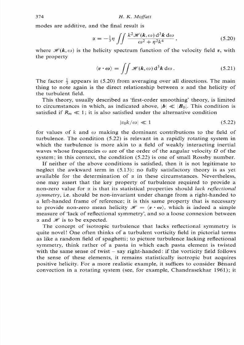
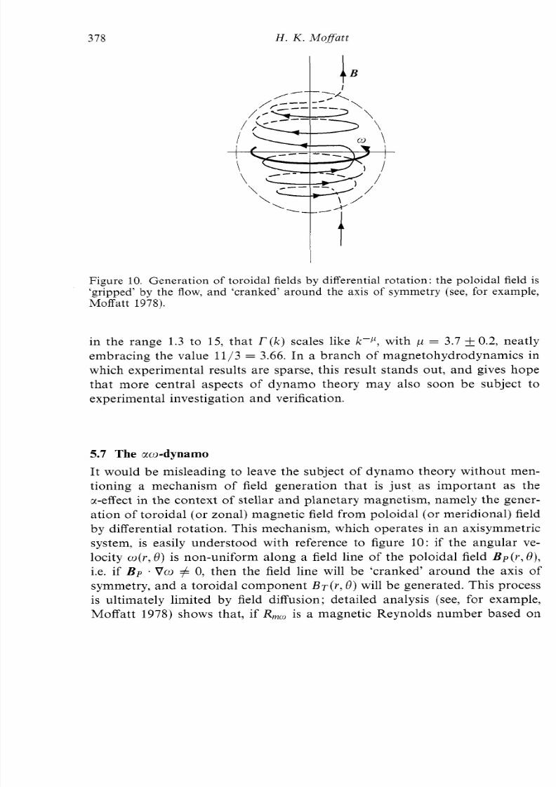
Figure 10. Generation of toroidal fields by differential rotation: the poloidal field is‘gripped’ by th e flow, and ‘cranked’ around the axis of symmetry (see, for example,Moffatt 1978).
in the ran ge 1.3 to 15, that r(k) cales like k W , with ,u = 3.7 0.2, neatly
embracing the value 11/3 = 3.66. In a branch of magnetohydrodynamics in
which experimental results are sparse, this result stands out, and gives hope
that more central aspects of dynamo theory may also soon be subject to
experime ntal investigation an d verification.
5.7 The aw-dynamo
It would be misleading to leave the subject of dynamo theory without men-
tioning a mechanism of field generation that is just as important as the
x-effect in the con text of stellar and p lanetary m agnetism, namely the gener-
ation of toroidal (o r zon al) m agnetic field from poloidal (o r me ridional) field
by differential rotation. This mechanism, which operates in an axisymmetric
system, is easily und erstood with reference to figure 10 : if the angu lar ve-
locity w ( r ,Q ) is non-uniform along a field line of the poloidal field B p ( r , Q ) ,i.e. if B p . Vw # 0, then the field line will be ‘cranked’ aro un d the axis of
symmetry, an d a toroidal com ponent BT ( r ,Q ) will be generated. This process
is ultimately limited by field diffusion; detailed analysis (see, for example,
M offatt 1978) shows tha t, if R,, is a magnetic Reynolds number based on
8/3/2019 H.K. Moffatt- Reflections on Magnetohydrodynamics
http://slidepdf.com/reader/full/hk-moffatt-reflections-on-magnetohydrodynamics 33/45
7 Reflections on hfugnetohydrodynumics 379
the strength and scale of the differential rotation, then B T saturates at a
This of course is on the assumption that, through some other mechanism,
the field B p is itself maintained at a steady level. There is no axisymmetric
mechanism that can achieve this (Cowling 1934), and it is of course here
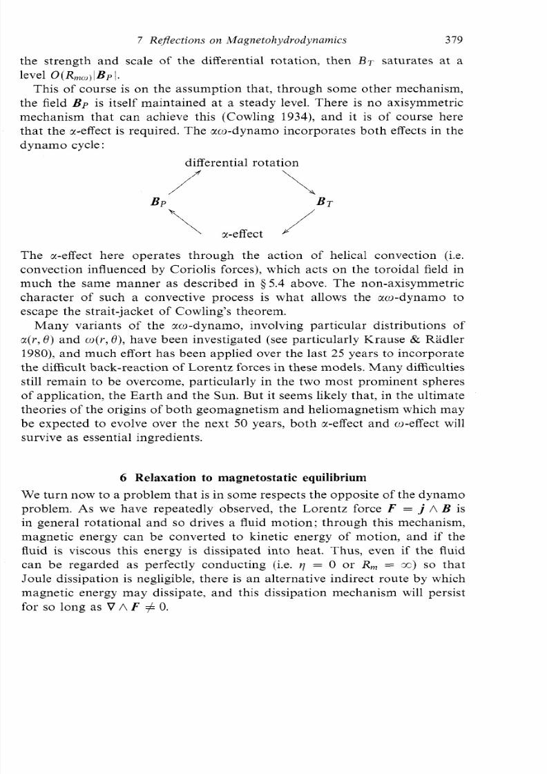
that the a-effect is required. The 8cio-dynamo ncorp orates both effects in the
dyn am o cycle :
differential ro tationf \
level 0 ( R m )BP I *
a-effect JThe ct-effect here operates through the action of helical convection (i.e.
convection influenced by Coriolis forces), which acts on the toroidal field in
much the same manner as described in $5.4 above. The non-axisymmetric
character of such a convective process is what allows the cto-dynamo to
escape the strait-jacket of Cowling’s theorem.
Many variants of the xo-dynamo, involving particular distributions of~ ( r ,) and o ( r ,0), have been investigated (see particularly Krause & Radler
1980), and m uch effort has been applied over the last 25 years to incorporate
the difficult back-reaction of Lo rentz forces in these models. Ma ny difficulties
still remain to be overcome, particularly in the two most prominent spheres
of application, the E ar th a nd the Sun. But it seems likely that , in the ultima te
theories of the origins of both geom agnetism and heliomagnetism which may
be expected to evolve over the next 50 years, both a-effect and co-effect will
survive as essential ingred ients.
6 Relaxation to magnetostatic equilibrium
We turn now to a problem that is in some respects the opposite of the dynam o
problem. As we have repeatedly observed, the Lorentz force F = j A B is
in general rotational and so drives a fluid motion; through this mechanism,
magnetic energy can be converted to kinetic energy of motion, and if the
fluid is viscous this energy is dissipated into heat. Thus, even if the fluidcan be regarded as perfectly conducting (i.e. y~ = 0 or R, = x) o that
Joule dissipation is negligible, there is an alternative indirect route by which
magnetic energy may dissipate, and this dissipation mechanism will persist
for so long as V A F # 0.
8/3/2019 H.K. Moffatt- Reflections on Magnetohydrodynamics
http://slidepdf.com/reader/full/hk-moffatt-reflections-on-magnetohydrodynamics 34/45
380 H . K . MofSatt
Insofar as the fluid is perfectly conducting however, the topology of the
magnetic field is conserved du ring this ‘relaxation’ process; in par ticu lar, all
links an d kn ots present in the m agnetic flux tubes a t the initial instant t = 0
are present at least for all finite times t > 0. It is physically obvious that the
magnetic energy cannot decay to zero under such circumstances; the only
alternative possibility is that the field relaxes to an equilibrium compatible
with its initial topology and for which V A F = 0. In such a state
F = j A B = V p , (6.1)
i.e. the Lorentz force is balanced by a pressure gradient and the fluid is at rest:
the field is in m agnetostatic equilibrium (see, for exam ple, Biskamp 1993).
We shall look more closely at the details of this process in the followingsubsections; for the moment it need merely be noted that we are faced
here with an intriguing class of problems of variational type: to minimize
a positive functional of the field B (here the magnetic energy) subject to
conservation of the field topo logy ; this topological con straint is conveniently
captured by the requirement that only frozen-field distortions of B , i.e. those
governed by the frozen-field equation
2 B- V A ( U A B ) ,2 t
are to be considered. We know that this equation guarantees conservation
of magnetic helicity Z lv (62.2 above ); bu t since (6.2) tells us tha t the field B
in effect deforms with the flow, all its topological properties (i.e. those prop-
erties that are invariant under continuous deformation) are automatically
conserved under this evolution.
We may look at this also from a Lagrangian point of view. Let the
Lagrangian particle path associated with the flow ~ ( x ,) be given by
x + X ( X , ) , 2 X / & = U , X ( X ,0) = x . (6.3)
Then the L agrangian statement equivalent to (6.2) is
where p is the density field. The deformation tensor ?Xi/O^xj encapsulates
both the rotation and stretching of the field element of B as it is trans-ported from x to X in time t . If the fluid is incompressible, then of course
p ( X )= p ( x ) .No te tha t (6.3) is a family of map pings continuously d epen den t
on the parameter t , and being the identity mapp ing at t = 0 ; in the language
of topology, it is an ‘isotopy’.
8/3/2019 H.K. Moffatt- Reflections on Magnetohydrodynamics
http://slidepdf.com/reader/full/hk-moffatt-reflections-on-magnetohydrodynamics 35/45
7 Reject ions on Magnetohydvodynamics 38 1
6.1 The structure of magnetostatic equilibrium states
Equation (6.1) places a strong constraint on the structure of possible mag-
netostatic equ ilibria; it implies tha t
j Vp = 0 and B - Vp = 0, (6.5)
so tha t, in any region w here Vp # 0, bo th the curre nt lines (j-lin es) and field
lines (B-lines) must lie on surfaces p = const.
0, it follows from (6.1) tha t j is parallel to B,
i.e.
In any region where Vp
j = y(x)B (6.6)
for some scalar field y(x).The field B is then desc ribed as ‘force-free’ in thisregion. There is a considerable literature devoted to the subject of force-free
fields (see particularly M ars h 1996); here we simply note th at, on taking the
divergence of (6.6) and using V j = V B = 0, we obtain
B * V y= 0 , (6.7)
so that now the B-lines lie on surfaces y = const. The only possible escape
from this (topological) constraint is when Vy 0 and y = const. The field B
is then a ‘Beltrami’ field. We have seen one exam ple in (5.25) above; a moregeneral field satisfying V A B = yB may be constructed as a superposition of
circularly polarized Fourier modes in the form
where I$ = k/ lk l and k . $ ( k )= 0. With such a field, the B-lines are no longer
constrained to lie on surfaces; the p articular field (5.25) exhibits the property
of chaotic w andering of B-lines (H eno n 1 966; Arn old 1966; Do m bre et al.
1986), an d it may be conjectured th at this a generic property of force-free
fields of the general form (6.8).
6.2 Magnetic relaxation
Supp ose now th at incompressible fluid is contained in a dom ain 2 ith fixed
rigid boundary $2.or the reasons already indicated, let us suppose that
this fluid is viscous and perfectly conducting. Such a combination of fluidproperties is physically artificial; but no matter - this is a situation where
the end justifies the means! We suppose that at t = 0 the fluid is at rest
and that it supports a magnetic field Bo(x) where I I . Bo = 0 on 29.Clearly
this condition of tangency of the field at the surface 2 9 persists under the
I
8/3/2019 H.K. Moffatt- Reflections on Magnetohydrodynamics
http://slidepdf.com/reader/full/hk-moffatt-reflections-on-magnetohydrodynamics 36/45
382 H . K . M o f a t t
subsequent evolution. This evolution is governed by equation (6.2) together
with (3.3 ), or equivalently
( E + u + V U ) = - , V p + - j A B + v V ’ u .1
PThe velocity U satisfies the no-slip condition U = 0 on 29.
From (6.2) and (6.9) we m ay easily cons truct an energy equation. Let
the magnetic and kinetic energies. Then this energy equation is
(6.10)
(6.11)
where o = V A U . As expected, the sole mechanism of d issipation is viscosity.
Now let us suppose that the topology of the initial field B o ( x ) is non-
trivial, and in particular, that its helicity X A ~s non-zero. This helicity is
conserved under (6.2); moreover non-zero helicity clearly implies a positive
lower bound for magnetic energy (Arnold 1974):
M 2 L Z 1 1 X W l > (6.12)
where L g is a constant with the dimensions of length; this constant is
determined by the geometry of 2 nd can normally be interpreted as a
represen tative linear scale of 9.
Since M +K is mo notonic decreasing (by (6.11)) and bou nded below (by
(6.12)), t must tend to a positive con stan t; hence the right-ha nd side of (6.11)
tends to zero as t + E. rovided no singularity of cr) develops, it follows that
cr) + 0 for all x E 9 s t + E; it is then not difficult to show that, under
the no-slip condition on $9,-+ 0 also for all x E 9,.e. the limit state is
indeed magnetostatic. Thus, as t + x, + B E ( x ) , + E ( x ) ,where
j E I P \ B E= V p E . (6.13)
This evolutiona ry process may be represented p ictorially by a ‘trajectory’$
in the function space F f solenoidal vector fields of finite energy (figure 11).
This trajectory is confined to a subspace 9 f those fields that can be
obtained from B o ( x ) by isotop ic (frozen-field) deform ation . Such a subspace,
described as ‘isomagnetic’ is indicated as a surface in figure 11, bu t this is amisleading simplification, since it is in fact infinite-dimensional. Nevertheless,
9 ay be thought of as ‘foliated’ by such isomagnetic subspaces, the fields
on any such subspace being ‘topologically accessible’ one from another by
isotopic deformation. This concept of an ‘isomagnetic subspace’ is closely
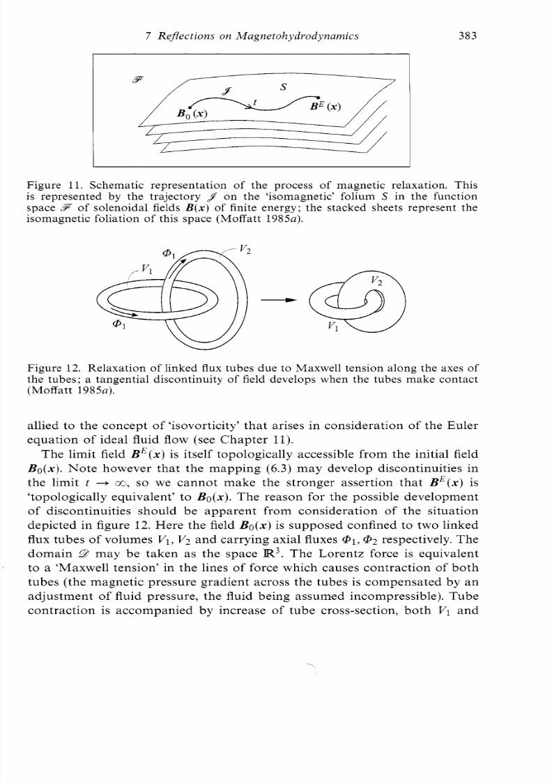
8/3/2019 H.K. Moffatt- Reflections on Magnetohydrodynamics
http://slidepdf.com/reader/full/hk-moffatt-reflections-on-magnetohydrodynamics 37/45
7 Ref lec t ions on Magnetohydrodynamicsa83
Figure 11. Schematic representation of the process of magnetic relaxation. Thisis represented by the trajectory $ on the ‘isomagnetic’ folium S in the functionspace 9 f solenoidal fields B ( x ) of finite energy; the stacked sheets represent the
isomagnetic foliation of this space (Moffatt 1 9 8 5 ~ ) .
Figure 12. Relaxation of linked flux tubes due to Maxwell tension along the axes ofthe tubes; a tangential discontinuity of field develops when the tubes make contact(Moffatt 1 9 8 5 ~ ) .
allied to the concept of ‘isovorticity’ that arises in consideration of the Euler
equ ation of ideal fluid flow (see Ch ap ter 11).The limit field BE(x)s itself topologically accessible from the initial field
Bo(x ) . Note however that the mapping (6.3) may develop discontinuities in
the limit t + a, o we cannot make the stronger assertion that B E ( x ) s
‘topologically equivalent’ to B o ( x ) .The reason for the possible development
of discontinuities should be apparent from consideration of the situation
depicted in figure 12. Here the field B o ( x ) is supposed confined to two linked
flux tubes of volumes V1,V2 and carrying ax ial fluxes @ I , @2 respectively. The
domain 2 may be taken as the space R3.The Lorentz force is equivalentto a ‘M axwell tension’ in the lines of force which causes con traction of bo th
tubes (the magnetic pressure gradient across the tubes is compensated by an
adjus tme nt of fluid pressure, the fluid being assumed incom pressible). Tube
contraction is accompanied by increase of tube cross-section, both V1 and
n
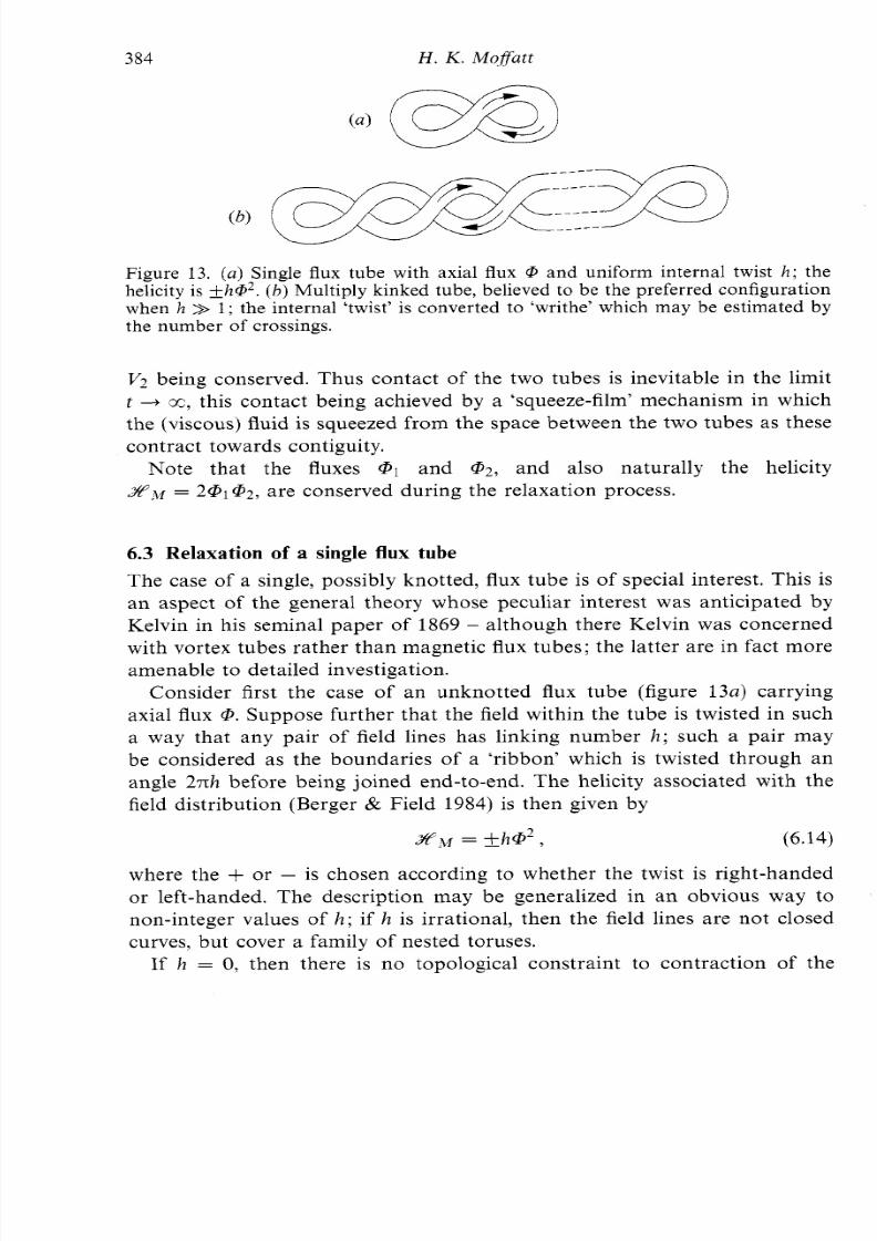
8/3/2019 H.K. Moffatt- Reflections on Magnetohydrodynamics
http://slidepdf.com/reader/full/hk-moffatt-reflections-on-magnetohydrodynamics 38/45
384 H. . Moffatt
Figure 13. (a) Single flux tube with axial flux @ and uniform internal twist h ; thehelicity is &hQ2. ( b ) Multiply kinked tube, believed to be the preferred configurationwhen h >> 1; the internal ‘twist’ is converted to ‘writhe’ which m ay b e estim ated bythe number of crossings.
V2 being conserved. Thus contact of the two tubes is inevitable in the limit
t --+ E, this con tact being achieved by a ‘squeeze-film’ mechanism in which
the (viscous) fluid is squeezed from the space between the two tubes as these
contract towards contiguity.
Note that the fluxes @1 and @ 2 , and also naturally the helicity
X .w = 2@1@2, are conserved during the relaxation process.
6.3 Relaxation of a single flux tube
The case of a single, possibly knotted, flux tube is of special interest. This is
an aspect of the general theory whose peculiar interest was anticipated by
Kelvin in his seminal paper of 1869 - although there Kelvin was concerned
with vortex tubes rather than magnetic flux tubes; the latter are in fact more
amenable to detailed investigation.
Con sider first the case of an unk not ted flux tube (figure 13a) carrying
axial flux @. Suppose further that the field within the tube is twisted in sucha way that any pair of field lines has linking number h ; such a pair may
be considered as the bound aries of a ‘ribbon’ which is twisted through an
angle 27th before being joined end-to-end. The helicity associated with the
field distribution (Berger & Field 1984) is then given by
2 , ~+_hQ2, (6.14)
where the + or - s chosen according to whether the twist is right-handed
or left-handed. The description may be generalized in an obvious way to
non-integer values of h ; if h is irrational, then the field lines are not closed
curves, but cover a family of nested toruses.
If h = 0, then there is no topological constraint to contraction of th e
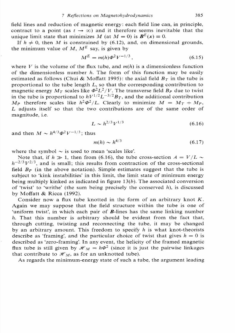
8/3/2019 H.K. Moffatt- Reflections on Magnetohydrodynamics
http://slidepdf.com/reader/full/hk-moffatt-reflections-on-magnetohydrodynamics 39/45
7 Repections on Magnetohydrodynamics 38 5
field lines and reduction of magnetic energy: each field line can, in principle,
contract to a point (as t -+ x) nd it therefore seems inevitable that the
unique limit state that minimizes M (a t M = 0) is B E ( x )= 0.
If h # 0, then M is constrained by (6.12), and, on dimensional grounds,
the minimum value of M , M E say, is given by
M E = WI ( ~) Q ’ I / - ~ ’ ~ , (6.15)
where V is the volume of the flux tube, and m ( h ) s a dimensionless function
of the dimensionless number h. The form of this function may be easily
estimated as follows (Chui & M offatt 199 5): the axial field B T in the tube is
propo rtional to the tube length L, so tha t the corresponding con tribution to
mag netic energy M T scales like Q2L2/V. he transverse field Bp due to twist
in the tube is proportional to hV1 /2L -3 /2B~ ,nd the additional contribution
M p therefore scales like h 2 Q 2 / L . Clearly to minimize M = M T + M p ,
L adjusts itself so that the two contributions are of the same order of
magnitude, i.e.
- 2 1 3 ~ 1 1 3 (6.16)
and then M - h4/3Q2V-1/3;hus
m ( h )-4I3 (6.17)
where the symbol - s used to mean ‘scales like’.
Note that, if h >> 1, then from (6.16), the tube cross-section A = V / L-hK2I3V2I3, nd is small; this results from contraction of the cross-sectional
field B p (in the above notation). Simple estimates suggest that the tube is
subject to ‘kink instabilities’ in this limit, the limit state of minimum energy
being m ultiply kinked as indicated in figure 13(b). The associated conversion
of ‘twist’ to ‘writhe’ (the sum being precisely the conserved h ) , is discussedby Moffatt & Ricca (1992).
Consider now a flux tube knotted in the form of an arbitrary knot K .
Again we may suppose that the field structure within the tube is one of
‘uniform twist’, in which each pair of B-lines has the same linking number
h. That this number is arbitrary should be evident from the fact that,
through cutting, twisting and reconnecting the tube, it may be changed
by an arbitrary amount. This freedom to specify h is what knot-theorists
describe as ‘framing’, an d the pa rticu lar cho ice of twist tha t gives h = 0 isdescribed as ‘zero-framing’. In any event, the helicity of the framed magnetic
flux tube is still given by HAu= hQ2 (since it is just the pairwise linkages
that contribute to XAu, s for an unkno tted tube).
A s regards the minimum-energy state of such a tube , the argum ent leading
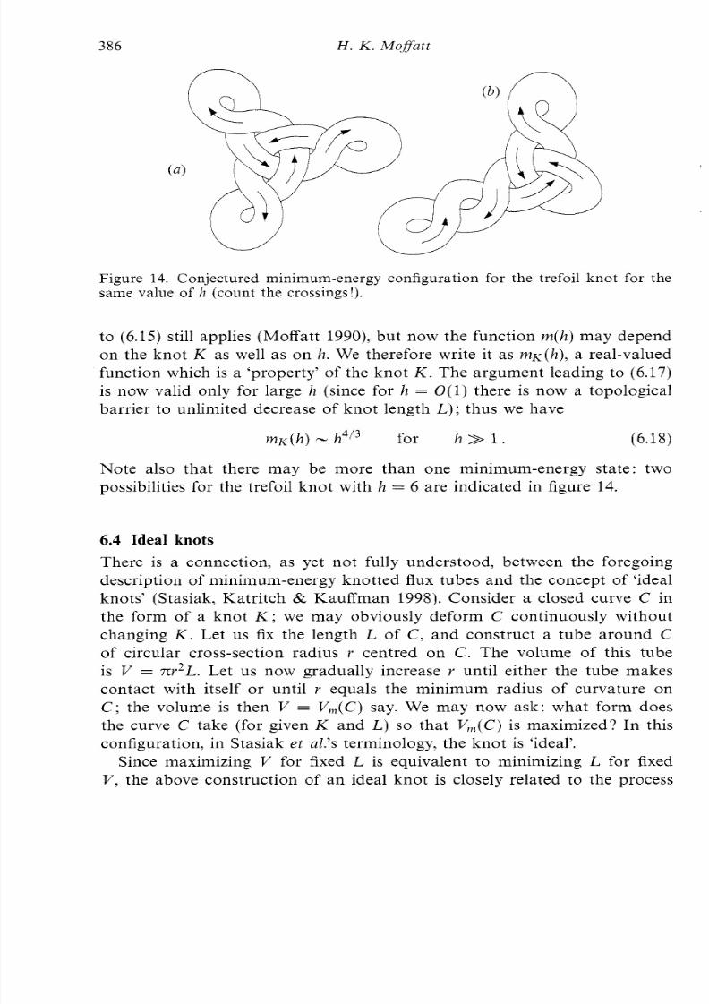
8/3/2019 H.K. Moffatt- Reflections on Magnetohydrodynamics
http://slidepdf.com/reader/full/hk-moffatt-reflections-on-magnetohydrodynamics 40/45
386 H . K . M o f a t t
Figure 14. Conjectured minimum-energy configuration for the trefoil knot for thesame value of h (count the crossings!).
to (6.15) still applies (Moffatt 1990), but now the function m ( h ) may depend
on the knot K as well as on h. We therefore write it as m ~ ( h ) , real-valued
function w hich is a ‘property’ of the kn ot K . The argument leading to (6.17)
is now valid only for large h (since for h = O(1) there is now a topological
barrier to unlimited decrease of knot length L ) ; hus we have
m K ( h )- 4I3 for h >> 1. (6.18)
Note also that there may be more than one minimum-energy state: two
possibilities for the trefoil knot with h = 6 are indicated in figure 14.
6.4 Ideal knots
There is a connection, as yet not fully understood, between the foregoing
description of minimum-energy knotted flux tubes and the concept of ‘ideal
knots’ (Stasiak, Katritch & Kauffman 1998). Consider a closed curve C in
the form of a knot K ; we may obviously deform C continuously without
changing K . Let us fix the length L of C, and construct a tube around C
of circular cross-section radius r centred on C . The volume of this tube
is I/ = m2L. Let us now gradually increase r until either the tube makes
contact with itself or until r equals the minimum radius of curvature on
C ; the volume is then I/ = V,,(C) say. We may now ask: what form does
the curve C take (for given K and L) so that V,(C) is maximized? In this
configuration, in Stasiak et al.’s terminology, the knot is ‘ideal’.
Since maximizing V for fixed L is equivalent to minimizing L for fixed
V, the above construction of an ideal knot is closely related to the process
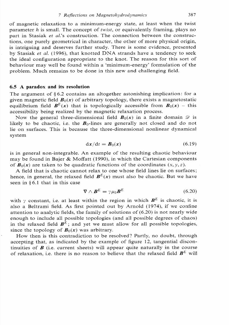
8/3/2019 H.K. Moffatt- Reflections on Magnetohydrodynamics
http://slidepdf.com/reader/full/hk-moffatt-reflections-on-magnetohydrodynamics 41/45
7 Reflections on Magnetohydrodynamics 387
of magnetic relaxation to a minimum-energy state, at least when the twist
parameter h is small. The concept of twis t , or equivalently framing, plays no
part in Stasiak et al.'s construction. The connection between the construc-
tions, one purely geom etrical in chara cter, the o ther of more physical origin,
is intriguing and deserves further study. There is some evidence, presentedby Stasiak et al. (1996), that knotted D N A strands have a tendency to seek
the ideal configuration appropriate to the knot. The reason for this sort of
behaviour may well be found within a 'minimum-energy' formulation of the
problem. Much remains to be done in this new and challenging field.
6.5 A paradox and its resolution
The argument of 5 6.2 contains an altogether astonishing implication: for a
given magnetic field B o ( x ) of arb itrary topology, there exists a magnetostatic
equilibrium field B E ( x ) hat is topologically accessible from B o ( x ) - this
accessibility being realized by the magnetic relaxation process.
Now the general three-dimensional field B o ( x ) in a finite domain 9 s
likely to be chaotic, i.e. the Bo-lines are generally not closed and do not
lie on surfaces. This is because the three-dimensional nonlinear dynamical
system
d x / d t = B o ( x ) (6.19)
is in general non-integrable. An example of the resulting chaotic behaviour
may be found in Bajer & M offatt (1990), in which the C artesian com ponen ts
of B o ( x ) are taken to be quadratic functions of the coordinates (x ,y , z ) .
A field that is chaotic cannot relax to one whose field lines lie on surfaces;
hence, in general, the relaxed field B E ( x )must also be chaotic. But we have
seen in $ 6 .1 tha t in this caseV A BE= " / , jBE (6.20)
with y constant, i.e. at least within the region in which BE is chaotic, it is
also a Beltram i field. As first pointed ou t by A rno ld (197 4), if we confine
atten tion to analytic fields, the fam ily of so lutions of (6.20) is no t nearly wide
enough to include all possible topologies (and all possible degrees of chaos)
in the relaxed field B E ; nd yet we must allow for all possible topologies,
since the topology of B o ( x ) was arbitrary.How then is this contradiction to be resolved? Partly, no doubt, through
accepting that, as indicated by the example of figure 12, tangential discon-
tinuities of B (i.e. curren t sheets) will ap pe ar quite naturally in the course
of relaxation, i.e. there is no reason to believe that the relaxed field BE will
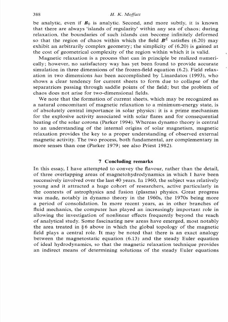
8/3/2019 H.K. Moffatt- Reflections on Magnetohydrodynamics
http://slidepdf.com/reader/full/hk-moffatt-reflections-on-magnetohydrodynamics 42/45
388 H . K. MofSatt
be analytic, even if Bo is analytic. Second, and more subtly, it is known
that there are always ‘islands of regularity’ within any sea of chaos; during
relaxation, the boundaries of such islands can become infinitely deformed
so that the region of chaos within which the field B E satisfies (6.20 ) may
exhibit an arbitrarily complex geometry; the simplicity of (6.20) is gained atthe cost of geometrical complexity of the region within which it is valid.
Magnetic relaxation is a process that can in principle be realized numeri-
cally; however, no satisfactory way has yet been found to provide accurate
simulation in three dimensions of the frozen-field equation (6.2). Field relax-
ation in two dimensions has been accomplished by Linard atos (1993), who
shows a clear tendency for current sheets to form due to collapse of the
separatrices passing through saddle points of the field; but the problem of
chaos does not arise for two-dimensional fields.We note that the formation of current sheets, which may be recognized as
a natural concomitant of magnetic relaxation to a minimum-energy state, is
of absolutely central importance in solar physics: it is a prime mechanism
for the explosive activity associated with solar flares and for consequential
heating of the so lar corona (Parker 1994). W hereas dy nam o theory is central
to an understanding of the internal origins of solar magnetism, magnetic
relaxation provides the key to a proper understanding of observed external
magnetic activity. The two process, bo th fund am ental, are complem entary in
more senses tha n one (P arker 1979; see also Priest 1982).
’
7 Concluding remarks
In this essay, I have attempted to convey the flavour, rather than the detail,
of three overlapping areas of magnetohydrodynamics in which I have been
successively involved over the last 40 years. In 1960, the subject was relatively
young and it attracted a huge cohort of researchers, active particularly in
the contexts of astrophysics and fusion (plasma) physics. Great progress
was made, notably in d yn am o theory in the 1960s, the 1970s being more
a period of consolidation. In more recent years, as in other branches of
fluid mechanics, the computer has played an increasingly important role in
allowing the investigation of nonlinear effects frequently beyond the reach
of analytical study. Some fascinating new areas have emerged, most notably
the area treated in $ 6 above in which the global topology of the magneticfield plays a central role. It may be noted that there is an exact analogy
between the magnetostatic equation (6.13) and the steady Euler equation
of ideal hydrodynamics, so that the magnetic relaxation technique provides
an indirect means of determining solutions of the steady Euler equations
8/3/2019 H.K. Moffatt- Reflections on Magnetohydrodynamics
http://slidepdf.com/reader/full/hk-moffatt-reflections-on-magnetohydrodynamics 43/45
7 Reflections on Magnetohydrodynamics 389
of arbitrary streamline topology (Moffatt 198.5~).There is a rich interplay
between M H D an d ‘ordinary’ fluid dynamics that stems from this analogy,
in subtle conjunction with the (different) analogy between (2.4) and (2.6).
Magnetohydrodynamics is a richly rewarding field of study, not only in its
own right, but also through the illumination of more classical areas of fluiddynamics that this interplay provides.
References
A L F V ~ N ,. 1950 Cosmical Electrodynamics. Oxford University Press.ARNOLD, . I. 1966 Su r la topologie des kcoulements stationna ires des fluides parfaits.
C. R. Acad. Sci. Paris 261, 17-20.
ARNOLD, . I. 1974 The asymptotic Hopf invariant and its applications. In Proc.Summer School in Diferen tial Eq uations, Erevan 1974. Armenian SSR Acad. Sci.[English transl: Sel. Mat h. Sou. 5 (1986), 327-3451.
ARNOLD,. I. & KHESIN, . A. 1998 Topological Methods in Hydrodynamics. Springer.BAJER,K . & MOFFATT, . K . 1990 O n a class of steady confined Stokes flows with
BATCHELOR,. K. 1950 O n the spontane ous magnetic field in a conducting liquid in
BERGER,M . A. & FIELD, . B. 1984 The topological properties of magnetic helicity.
BISKAMP, . 1993 Nonlinear Magnetohydrodynamics. Cambridge University Press.BOJAREVIES,., FREIBERGS,A., SHILOVA,. I. & SHCHERBININ,. V. 1989 Electrically
BRAGINSKII,. I. 1964 Theory of the hydromagnetic dynamo. Sou. Phys . JE TP 20,
BRAUNBEK,W. 1932 Eine neue Methode electrodenloser Leitfahigkeitsmessung.
CHANDRASEKHAR,. 1961 Hydrodynamic and Hydromagnetic Stability. Clarendon.CHILDRESS,. & GILBER T, . D . 1995 Stretch, T wi st, Fold: the Fast Dynam o. Springer.CHUI,A. Y. K. & MOFFATT, . K . 1995 Th e energy an d helicity of knotted magnetic
COOK,A. H. 1980 Interiors of the Planets. Cambridge University Press.COW LING , . G . 1934 The magnetic field of s unspo ts. Mon. No t . R . AstrON. Soc. 94,
COWLING, . G. 1957 Magnetohydrodynamics. Interscience; 2nd Edn 1975, AdamHilger Ltd., Bristol.
DOM BRE ,., FRISCH,U, , GRE E NE ,. M ., H ~ N O N , ., M E H R ,A. & SOWARD, . M .1986 Chaotic streamlines in the ABC flows. J . Fluid Mech. 167, 353-391.
DAVIDSON,. A., KIN NE AR , ., LINGWOO D, . J., SHORT,D. J. & H E, X. 1999 Therole of Ekman pumping and the dominance of swirl in confined flow driven by
Lorentz forces. Eur. J . Mech. BIFluids 18 , 693-711.GOLITSIN, . 1960 Fluctuations of magnetic field and current density in turbulent
flows of weakly conducting fluids. Sou. Phys. Dokl. 132, 315-318.H ~ N O N ,. 1966 Sur la topologie des lignes de cou ran t dan s un cas particulier. C. R .
Acad. Sci. Paris A 262, 312-314.JACOBS,. A. 1984 Recersals of the Earth ’s Ma gne tic Field. Ada m Hilger Ltd., Bristol.
chaotic streamlines. J . Fluid Mech. 212, 337-363.
turbulent motion. Proc. R. Soc. Lond. A 201, 405-416.
J. Fluid Mec h. 147, 133-148.
Induced Vortical Flows. Kluwer.
1462-147 1.
Z . Phys. 73, 312-334.
flux tubes. Proc. R. Soc. Lond. A 451, 609-629.
39-48.
8/3/2019 H.K. Moffatt- Reflections on Magnetohydrodynamics
http://slidepdf.com/reader/full/hk-moffatt-reflections-on-magnetohydrodynamics 44/45
390 H . K . Moffatt
KELVIN, ORD th en W. THOMSON)869 On vortex motion. Trans. R. Soc. Edin., 25,
KRAUSE,F. & RADLER,K.-H. 1980 Magnetohydrodynamics and Dynamo Theory.
LIXARDATOS,. 1993 Determination of two-dimensional magnetostatic equilibria
MARSH,G. E. 1996 Force-free Magnetic Fields: Solutions, Topology and Applications.
M EST EL, . J. 1982 M agnetic levitation of liquid metals. J . Fluid Mech. 117, 27-43.MOFFATT, . K. 1961 The amplification of a weak applied magnetic field by turbu-
lence in fluids of moderate conductivity. J . Fluid Mech. 11, 625-635.MOFFATT, . K. 1965 On fluid flow induced by a rotating magnetic field. J . Fluid
Mech. 22, 521-528MOFFATT, . K. 1967 On the suppression of turbulence by a uniform magnetic field.
J . Fluid Mech. 28, 571-592.MOFFATT, . K. 1969 The degree of knottedness of tangled vortex lines. J . Fluid
Mech. 35, 117-129.MOFFATT, . K. 1978 Magn etic Field G eneratio n in Electrically Cond ucting Fluids.
Cambridge University Press.MOFFATT, . K. 1985a Magnetostatic equilibria and analogous Euler flows of arbi-
trarily complex topology. Part 1. Fundamentals. J . Fluid Mech. 159, 359-378.MOFFATT, . K . 19852, Hig h frequency excitation of liquid metal systems. In Metal-
lurgical Applications of Magnetohydrodynamics (ed. H. K. Moffatt & M . R. E.Proctor), pp. 180-189. Metals Society, London.
MOFFATT, . K . & PROCTOR,M . R . E. (Eds.) 1984 Metallurgical Applications ofMagnetohydrodynamics. Metals Society, Lo ndo n.MOFFATT, . K. 1990 The energy spectrum of knots and links. Nature 347, 367-369.MOFFATT, . K . & RICCA,R . L. 1992 Helicity an d the CglugHreanu invariant. Proc.
MOREAU, . 1990 Magnetohydrodynamics. Kluwer.NORTHRUP,. E 1907 Some newly observed manifestations of forces in the interior
ODIER,P., PINTOX, .-F. & FAUVE,S. 1998 Advection of a magnetic field by a
PAR KER, . N. 1955 Hydrom agnetic dy nam o models. Astrophys. J . 122, 293-3 14.PARKER, . N . 1979 Cosmical Magnetic Fields. Clarendon.PARKER,. N . 1994 Spontaneous Current Sheets in Ma gnetic Fields. Oxford University
PRIEST, . R. 1982 Solar Magnetohydrodynamics. D. Reidel.RICHARDSOK,. F. 1922 Weather Prediction by Numerical Process. Cambridge Uni-
SCH USTE R, . 1912 A critical exam ination of the possible causes of terrestrial
SKEYD,A. D. & MOFFATT, . K. 1982 Fluid-dynamical aspects of the levitation
STAS IAK, ., KATRITCH, ., BEDKAR,., MICHOUD,D. & DUBOCHET,. 1996 Elec-
STASIAK, ., KATRITCH,. & KAUFFMAN,. H. 1998 Ideal Knots. World Scientific.STEEKBECK,M., KRAUSE,F. & RADLER,K.-H. 1966 Berechnung der mittleren
217-260.
Pergamon.
and analogous Euler flows. J . Fluid Mech. 246, 569-591.
World Scientific.
R . Soc. Lond. A 439, 4 1 1 4 2 9 .
of an electric conductor. Phys. Rev. 24, 474-497.
turbulent swirling flow. Phys. Rev. E 58, 7397-7401.
Press.
versity Press.
magnetism. Proc. Phys. Soc. Lond. 24, 121-137.
melting process. J . Fluid Mech. 117, 45-70.
trophoretic mobility of DNA knots. Nature 384, 122.
8/3/2019 H.K. Moffatt- Reflections on Magnetohydrodynamics
http://slidepdf.com/reader/full/hk-moffatt-reflections-on-magnetohydrodynamics 45/45
7 Re jec tion s on Magnetohydrodynamics 391
Lorentz-Feldstarke fur ein elektrisch leitendes Medium in turbulenter, durchCoriolis-Krafte beeinfluster Bewegung. 2. Naturforsch. 21a, 369-376.
VAINSHTEIN,. I. & ZELDOVICH,A.B. 1972 Origin of magnetic fields in astrophysics.
WOLTJER, . 1958 A theorem on force-free magnetic fields. Proc. Nut1 Acad. Sci. 44,
ZELDOVICH,A. B., RUZMAIKIN,. A. & SOKOLOFF,. D. 1983 Magnetic Fields in
SOU.Phys. USP.15, 159-172.
4 8 9 4 9 1.
Astrophysics. Gordon and Breach.
Isaac Newton Institute f o r Mathematical Sciences, University of Cambridge,20 Clarkson Roa d, Cambridge C B3 OEH, U K