History of Mathematics

Final Papers

Juniata College

Fall 2012

Dr. John Bukowski

Contents:

1. Mayan Mathematics

Nick Donlan

2. Pascal’s Triangle

Kevin Snyder

3. The Origins of Probability Theory!

Amy Ankney

4. James Stirlin!g an!d N!umbers of the First an!d Secon!d Kin!d

Matt Johann

5. Seven Bridges of Königsberg: An Eulerian Trail

Cody Johnson

6. Lloyd Shapley and His Work on Game Theory

Steve Kidhardt

7. The Four Color Problem

Melissa Stanton

Nick Donlan

History of Math

Dr. Bukowski

12/13/12

Mayan Mathematics

When people think about pre-Columbian American cultures, three civilizations tend to

come to mind. The first of these civilizations is the Aztecs who dominated most of central-south

America from the 14th

to 16th

centuries. Another is the Incas, who were the largest of the three

civilizations and came from the highlands of Peru in the early 13th

century. However, the third,

and oldest, of the three was the Mayans. The Mayans were first established around 2000 BC, but

they did not reach their pinnacle until around 250-900 AD. The Mayans are known for many

things including their art, architecture, astronomical developments, and calendar. They are also

the only pre-Columbian American civilization that developed a fully written language. However,

it was their revolutionary mathematics that led to the Mayans’ most famous developments.

In 1505, Hernan Cortes sailed from Spain and landed in Hispaniola, which is modern day

Santo Domingo (the capital and largest city in the Dominican Republic). Cortes had heard the

stories of Columbus’s voyages to the “New World” and became very intrigued by the prospect of

what lay in these new lands. Wanting to see these lands for himself, Cortes sailed to and lived in

Hispaniola for a few years. Eventually he sailed to Cuba in 1511 with aspirations to conquer the

land and its people. He was ultimately successful and elected leader of Santiago twice. However,

he soon had aspirations for bigger and better things. So, on February 18, 1519, with an army of

11 ships, 508 soldiers, 100 sailors, and 16 horses, Cortes made his way to the coast of the

Yucatan peninsula, which is modern day Southeastern Mexico. He eventually landed on the

Northern coast, at the city of Tabasco. Cortes was ready for a fight from the natives, but he

surprisingly met very little resistance. In fact, not only did he meet virtually no resistance, they

all but welcomed Cortes with open arms. They showered him with many gifts, and he met his

eventual wife, Malinche, here as well. These people that Cortes had landed upon and conquered

in Tabasco were the descendants of the ancient Mayans.

When studying Mayan culture and more specifically their mathematics, it is important to

note how knowledge of the Mayans and their achievements were made know to the rest of the

world. Diego de Landa was a Spanish monk who belonged to the Franciscan order. When he was

seventeen, he asked to be sent to the “New World” as a missionary. After gaining permission, he

landed in the Yucatan Peninsula, where these Mayan descendants lived. He did his best to

protect the indigenous people from new Spanish rulers, such as Cortes. He visited many of the

Mayan cities and tried to learn as much about the people and their culture as he could, during his

time with them. However, the one aspect of the people’s culture that Landa absolutely abhorred

was their religious practices. Landa was obviously a very devout Christian, and to Landa, the

Mayan religion was “the devil’s work” (Ifrah). Their religion consisted of a series of

hieroglyphics and icons. Because of this, Landa ordered that all idols, religious works, and

anything else related to the Mayan religion, be burned. However, for some reason, Landa then

wrote and published a book in 1566, Relacion de las cosas de Yucatan, which gave detailed

accounts of everything Mayan, including religion. It described their hieroglyphics, customs,

temples, religious practices, and the overall history of the Mayans. Landa’s book is a major

reason why the world knows so much about the Mayan civilization today.

However, despite Landa’s desperate attempts to eradicate many of the records of the

Mayans, a small number of original Mayan documents survived. These also help to educate

people about Mayan culture, society, and customs. The three most famous are the Paris Codex,

the Madrid Codex, and the Dresden Codex. The Paris Codex is housed in the Bibliotheque

nationale in Paris. The Madrid Codex is housed in the American Museum in Madrid, and the

Dresden Codex, which is a piece on astronomy, is stored in the Sachsische Landesbibliothek

Dresden.

The ancient Mayans had a very sophisticated civilization for the time. They built very

large cities, equipped with such fixtures as temples, palaces, shrines, plazas, and giant basins to

hold rainwater. Astronomer priests ruled Mayan people using religion. Their farming system was

very sophisticated, with raised fields and intricate irrigation systems. They were used to provide

food for the massive amounts of people that lived in the cities. A common culture, calendar, and

religious practice held the mighty and vast Mayan civilization together, but in order to develop a

calendar and the astronomy behind their religious practices, a very good grasp of mathematics

was required. The Mayans created a sophisticated number system more advanced than that of

any other civilization in the world.

Today, modern society for the most part uses a base ten system. There are also some uses

of a sexagesimal system, or a base sixty number system, in modern society as well. This stems

from the ancient Sumerians and Babylonians as they also used a base sixty system. There are

sixty seconds in a minute, sixty minutes in an hour, etc. Virtually no one uses a base twenty or

vigesimal system. However, this is precisely what the Mayans used. Although the reason why

they used twenty as their base cannot be proved, it is thought, with fairly decent certainty, that it

was because people counted using their fingers and toes. However, despite being a base twenty

system, the number five also played a major role in their number system. This can be attributed

to the number of fingers or toes on each hand or foot.

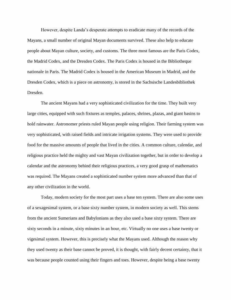
Somewhat surprisingly though, the Mayans only used three different symbols to represent

numbers. They used a system of dots, bars, and a symbol resembling a seashell. However, there

were two distinct features of the Mayans mathematics that set it apart from anything else in the

world during this time. First, they discovered the idea of zero (which they denoted with their

shell symbol) and second, their number system was positional in nature. The following is a

visual example, from the St. Andrews history of mathematics website, of the Mayan positional

number system:

However, despite this system being positional in nature, it is not a true positional number

system. In a true base twenty system, the first number of the system would signify the number of

units up to nineteen, the next would represent the number of “20’s” up to nineteen, and then the

next number would denote the number of 202 or 400’s up to nineteen. The Mayan system has a

slight variation. Their system starts the same with the first two places, but the third placeholder

in the Mayan system represents 360 instead of the 400 it would represent in a true base twenty

system. After the third place, the system continues just like any other base twenty number system.

So the fourth place denotes the number of 204 or 160,000 up to nineteen, the fifth place would

denote the number 205 or 3,200,000 up to nineteen, etc. For example [5;12;6;3;14] represents

This system was described in the Dresden Codex, and consequently the only system for

which written evidence exists. The irregularities in this system are attributed to needing to use

this number system for astronomical and calendar calculations, which do not fall perfectly into a

base twenty system. However, it was thought a second base twenty system, which was an actual

true vigesimal system, was used by merchants. This system also utilized special symbols for 20,

400, and 8000. Georges Ifrah, in his book A Universal History of Numbers: From Prehistory to

the Invention of the Computer, wrote “Even though no trace of it remains, we can reasonably

assume that the Maya had a number system of this kind, and that intermediate numbers were

figured by repeating the signs as many times as was needed.”

As previously mentioned, one of the main reasons the Mayans developed such a number

system was for the development of their calendar. There were influences from other directions

and sources, but the base twenty systems of the Mayans played a major role in the structure of

their calendar.

The Mayans actually had two main calendars, both of which they observed. The shorter

of the two is known as Tzolkin and consisted of 260 days. It was split into thirteen months with

twenty days in each month. The thirteen months were named after the thirteen gods of the Mayan

religion, and the twenty days were numbered from zero to nineteen. This makes the Mayan

number system’s influence on their calendar clear. Their second calendar consisted of 365 days

and was called the Haab. This calendar consisted of eighteen months and was more focused

around agricultural and religious events. Each month again consisted of twenty days numbered

from zero to nineteen. However, doing the math, eighteen multiplied by twenty is 360. Therefore,

there are five extra days left in the Haab calendar year. These extra five days made up a short

month called the Wayeb. The Mayans hated and feared the Wayeb. They considered it extremely

unlucky and did not wash, comb their hair, or do any work during these five days. It was also

believed that any child born during the Wayeb would have bad luck, remain poor, and generally

be very unhappy during their entire life.

Why the Mayans had a calendar based on 260 days is not entirely known. One theory is

the Mayans lived in a place that the sun was directly overhead every 260 days, with 105 days in

between periods. Another theory is that the Mayans had thirteen gods, and twenty was a man’s

number, so by giving each Mayan god a twenty-day month, it gave a ritual calendar consisting of

260 days.

Despite the reason for the two calendars, having them meant that they would coincide

with each other after 18,980 days (which equates to fifty-two years on the Haab, or seventy-three

years on Tzolkin). Another major aspect that contributed to the development of the calendar was

the synodic period of Venus. The Mayans noticed that Venus returned to the same position every

584 days. Therefore, after only two of the of the fifty-two year cycles, Venus would have made

sixty-five revolutions and end up at the original position. This extraordinary occurrence would

happen every 104 years and was marked by great celebrations.

There was also a third method of measuring time that the Mayan people used. Although it

wasn’t a calendar, it still utilized their extensive mathematics. It was an absolute timescale,

which began on a date from which days and times were measured going forward. The date most

often thought of as the start day, although not unanimous among scholars, is August 12, 3113 BC.

This method of counting days is known as the Long Count. The unique aspect of the Long Count

was that it was based on neither the Tzolkin nor the Haab. Instead, it is based on a year of 360

days. This shows the most likely reason for the departure of the number system from the true

vigesimal system; it was so that the system approximately represented years. Many examples of

the Long Count were found in Mayan cities and towns, such as the date a certain building was

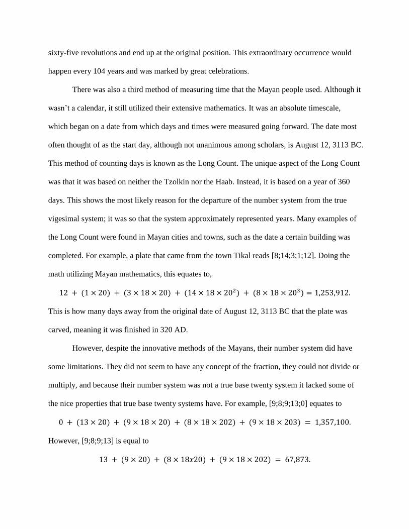
completed. For example, a plate that came from the town Tikal reads [8;14;3;1;12]. Doing the

math utilizing Mayan mathematics, this equates to,

This is how many days away from the original date of August 12, 3113 BC that the plate was

carved, meaning it was finished in 320 AD.

However, despite the innovative methods of the Mayans, their number system did have

some limitations. They did not seem to have any concept of the fraction, they could not divide or

multiply, and because their number system was not a true base twenty system it lacked some of

the nice properties that true base twenty systems have. For example, [9;8;9;13;0] equates to

However, [9;8;9;13] is equal to

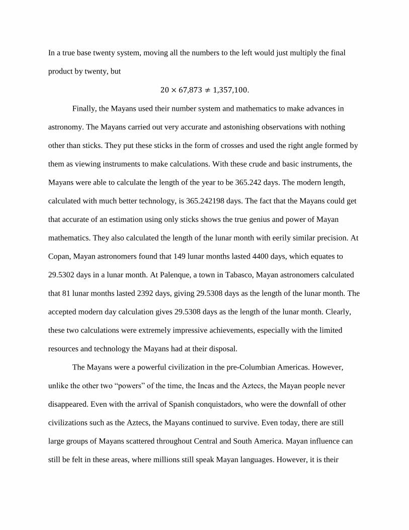
In a true base twenty system, moving all the numbers to the left would just multiply the final

product by twenty, but

.

Finally, the Mayans used their number system and mathematics to make advances in

astronomy. The Mayans carried out very accurate and astonishing observations with nothing

other than sticks. They put these sticks in the form of crosses and used the right angle formed by

them as viewing instruments to make calculations. With these crude and basic instruments, the

Mayans were able to calculate the length of the year to be 365.242 days. The modern length,

calculated with much better technology, is 365.242198 days. The fact that the Mayans could get

that accurate of an estimation using only sticks shows the true genius and power of Mayan

mathematics. They also calculated the length of the lunar month with eerily similar precision. At

Copan, Mayan astronomers found that 149 lunar months lasted 4400 days, which equates to

29.5302 days in a lunar month. At Palenque, a town in Tabasco, Mayan astronomers calculated

that 81 lunar months lasted 2392 days, giving 29.5308 days as the length of the lunar month. The

accepted modern day calculation gives 29.5308 days as the length of the lunar month. Clearly,

these two calculations were extremely impressive achievements, especially with the limited

resources and technology the Mayans had at their disposal.

The Mayans were a powerful civilization in the pre-Columbian Americas. However,

unlike the other two “powers” of the time, the Incas and the Aztecs, the Mayan people never

disappeared. Even with the arrival of Spanish conquistadors, who were the downfall of other

civilizations such as the Aztecs, the Mayans continued to survive. Even today, there are still

large groups of Mayans scattered throughout Central and South America. Mayan influence can

still be felt in these areas, where millions still speak Mayan languages. However, it is their

contributions to mathematics that really made the Mayans stand out in the world and led to many

of the developments and achievements that they are still known for today.

Bibliography

G Ifrah, A universal history of numbers : From prehistory to the invention of the

computer (London, 1998).

"Mayan Mathematics." Mayan Mathematics. N.p., n.d. http://www-history.mcs.st-

and.ac.uk/HistTopics/Mayan_mathematics.html. 12 Dec. 2012.

"Mayan Mathematics - The Story of Mathematics." Mayan Mathematics - The

Story of Mathematics. N.p., n.d. http://www.storyofmathematics.com/mayan.html. 12

Dec. 2012.

PASCAL’S TRIANGLE

KEVIN SNYDER

History:

Blaise Pascal was born June 19th, 1623 in Clermont, France, and died August 19th,

1662 in Paris, France[1]. He was only three years old when his mother passed away. His

father, Etienne Pascal, had to raise him along with three other children after that [1]. He

was the only son. His father was a local judge in Clermont [5] but later moved his family

to Paris because of work [1]. His father was a big influence on his son’s education. He did

not take the typical approach. He decided it was best to educate Blaise himself. His father

did not feel his son was going to be ready to learn math, however, so he did not have any

mathematical texts in the house. He wanted to hold off on math until Blaise was 15 years

old[1]. His father felt this way his son would not be stressed out over too much learning

[5].

This did not stop Pascal from being curious in the subject. At age 12, he was very

intrigued and curious about geometry [1]. He wanted to know more about the subject so

he asked his father. Once Pascal learned about the subject he wanted to learn so much

more about the subject. He then, on his own will, decided to give up his leisure time to

study math [5]. Within weeks of this, Pascal came up with a proof that the sum of the

angles in a triangle equaled the sum of two right angles [5]. From here, his father knew

that he needed to teach his son more about math. His father did a few things to help his

son further his education in mathematics. He let his son come to the Mersenne’s meetings

Date: December 13, 2012.1

2 KEVIN SNYDER

which were gatherings of a lot of mathematicians in Paris [5]. His father also gave his son

a copy of Euclid’s Elements which was a big inspiration for Pascal[1].

In 1639, the Pascal family was forced to move again. His father got a new job in Rouen,

France, where his father had been appointed as a tax collector [1]. Pascal wanted to help

his father with his work so he actually created one of the first mechanical calculators. This

calculator was specific to currency in France but was a big help to his father [1]. While in

Rouen, Pascal actually was starting to focus his studies on analytical geometry and physics.

He published one of his first works on atmospheric pressure [1]. He believed that there

was a vacuum that existed above the atmosphere [1]. This idea was not accepted by many

intellectuals around around the country. One in particular was Descartes. He visited Pascal

once and they argued for two days straight about whether there is actually a vacuum[1].

He wrote a few other papers containing information about the vacuum afterwards.

His father passed away in 1651. This day had a big effect on Pascal. After the death

of his father, he wrote to his siblings on the meaning of death and started to become very

religious and would change how he lived the rest of his life[1]. In 1654, Pascal wrote the

Treatise on the Arithmetical Triangle. He was not the first to discuss the topic however

his work is what made the triangle as popular as it is today [1]. His work led to Newton’s

discovery of the general binomial theorem for fractional and negative powers [1]. I will go

into further detail on this document later. After this, Pascal started to work with Fermat

on the foundation of the theory of probability [5]. The problem arose to them by a gambler.

The problem was, “Two players of equal skill want to leave the table before finishing their

game. Their scores and the number of points which constitute the game begin given, it

is desired to find in what proportion they should divide the stakes" [5]. Both Fermat and

Pascal worked on this problem and came up with the same conclusion using different proofs

[5].

Unfortunately for the math world, Pascal changed his focus of studies in 1654 [1]. This

happened after he experienced a life-altering accident. He was driving a four-in-hand

PASCAL’S TRIANGLE 3

carriage when the horses ran off. Pascal was saved, however, because of the brakes on the

carriage. He saw this as a sign from God [5]. He was from that moment on focused on

religion and stopped writing papers on math or physics.

He began publishing anonymous papers on religious concepts. They were called the

Provincial Letters and there were 18 of them. These papers were written to help protect

his friend who was in trouble for some of his religious work [1].

While on his religious quest to spread Christianity in 1658, Pascal started to have trouble

sleeping because of a toothache. He began to start thinking about math again and this

actually stopped him from having pain in his tooth. He saw this as a sign from God

that he should continue to think about math [5]. For the next eight days, he worked

on the geometry on the cycloid and published a paper on it [5]. This was Pascal’s last

mathematical work. A few years later he passed away in 1662 at the age of 39. He died

from an “intense pain after a malignant growth in his stomach spread to the brain" [1].

The Arithmetic Triangle:

As stated before Pascal wrote this document in 1954 while working with Fermat. His

work did not get published until after his death in 1665 [2]. Looking below we see the

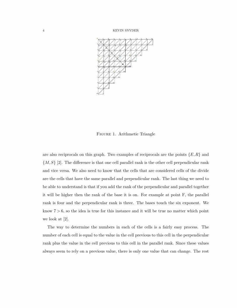
arithmetic triangle Pascal created [2].

The lines are put in a ranking system from a certain point. In Figure 1 that point is

point G. There are some properties of this triangle that we need to be able to understand

the consequences we want to draw from it [2]. Each square block is a cell. Each diagonal

line is called a base. The numbers going across the top and down the left sides of the cells

are the exponents of the lines. We see that the bases match up with the exponents. The

cells in the first row are considered to be in the same parallel rank [2]. It follows the same

pattern for each row. The exponent on the left of the row is considered to be its parallel

rank. The first column is all in the same perpendicular rank. This also is true as you move

through each column. The number on the top of the column is consider the perpendicular

rank. All points on the diagonal lines are considered to be on the same base [2]. There

4 KEVIN SNYDER

Figure 1. Arithmetic Triangle

are also reciprocals on this graph. Two examples of reciprocals are the points {E,R} and

{M,S} [2]. The difference is that one cell parallel rank is the other cell perpendicular rank

and vice versa. We also need to know that the cells that are considered cells of the divide

are the cells that have the same parallel and perpendicular rank. The last thing we need to

be able to understand is that if you add the rank of the perpendicular and parallel together

it will be higher then the rank of the base it is on. For example at point F, the parallel

rank is four and the perpendicular rank is three. The bases touch the six exponent. We

know 7 > 6, so the idea is true for this instance and it will be true no matter which point

we look at [2].

The way to determine the numbers in each of the cells is a fairly easy process. The

number of each cell is equal to the value in the cell previous to this cell in the perpendicular

rank plus the value in the cell previous to this cell in the parallel rank. Since these values

always seem to rely on a previous value, there is only one value that can change. The rest

PASCAL’S TRIANGLE 5

are set in stone due to this rule [2]. Since the triangle only needs one value to be able to

determine the rest of the values we call this triangle first cell a generator [2].

Consequences: From this information Pascal was able to come up with nineteen con-

sequences that always apply to this type of triangle. They are listed below with an expla-

nation for each that it is needed for [2]. For each of the consequences they pertain to all

arithmetic triangles.

1. All the cells of the first parallel rank and of the first perpendicular rank

are equal to the generator. This just says for our example since our generator is 1 this

means all the cells in the first row and first column are equal to 1.

2.Each cell is equal to the sum of all the cells of the preceding parallel rank,

comprehended from its perpendicular rank to the first inclusively. This was

shown above by how we obtain the value in each cell but it is more saying it is the sum

of all of them. For example, a cell in the fifth parallel rank is found by using the fourth

parallel rank which is found by using the third rank and so on and so forth.

3. Each cell equals the sum of all cells of the preceding perpendicular rank,

comprehended from its parallel rank to the first inclusively. This is the same as

above except instead of parallel it is perpendicular.

4. Each cell diminished by unity is equal to the sum of all cells which are

comprehended between its parallel rank and its perpendicular rank. This is

combining the the second and third consequence.

5. Each cell is equal to its reciprocal.

6. A parallel rank and a perpendicular which have one same exponent are com-

posed of cells all equals the ones to the others. This is true because when this case

happens the cells are reciprocals.

7. The sum of the cells of each base is double the cells of the base preceding.

Looking at our example the sum of the third base is 4. The sum of our fourth base is 8

which is twice the amount of the third base.

6 KEVIN SNYDER

8. The sum of the cells of each base is a number of the double progression

which begins with the unit of which the exponent is the same as the base. This

is similar to number seven except it says you start from the generator and the pattern will

always continue. Since the base is 1 this is true.

9. Each base diminished by unity is equal to the sum of all the preceding. This

just says we can get a sum of a base and divide it by 2 and get the sum of the previous

base. This is only true if the base is one. If it was something else then we would need to

say diminished by the generator.

10. The sum of as many contiguous cells as one will wish from its base, begin-

ning with an extremity, is equal to as many cells of the preceding base, plus

again as many except one. This is best shown by an example. If we looked at the third

base which contains 1,3,3,1 the sum of that is 8. Suppose we only want the first three so

1,3,3 which is 7. This says that if we look at the base above we get the same sum by taking

2∗ (1) + 2∗ (2) + 1 which in turn is true. This will always be true for any continuous cells

on the same base.

11. Each cell of the divide is double of that which precedes it in its perpendic-

ular or parallel rank. For instance the divide that contains a parallel and perpendicular

rank of 4 is equal to 20. If we look at the cell with the same perpendicular rank but the

previous parallel rank it is equal to 10. We see the same thing for the previous perpendic-

ular rank and the same parallel rank.

12. Two contiguous cells being in one same base, the superior is to the inferior

as the number of cells from the superior to the top of the base to the number

of cells from the inferior to the bottom inclusively. The best way to understand

this is by looking at the figure. The expression E is to C as 2 is to 3 is true. E has two

cells below it on the same base while C has three cells above it on the same base. We could

consider C superior to E in this case.

13. Two contiguous cells being in the same perpendicular rank, the inferior is

PASCAL’S TRIANGLE 7

to the superior as the exponent of the base of this superior to the exponent of

its parallel rank. Again an example from the diagram is helpful. We will say F is to C

as 5 is to 3. F is the inferior and C is the superior. 5 is the exponent of the base C and 3

is the parallel rank of C.

14. Two contiguous cells being in the same parallel rank, the greatest is to the

preceding as the exponent of the base of that preceding to the exponent of its

perpendicular rank. Looking at the diagram, we can say F is to E as 5 is to 2. F is

the greatest and E is the preceding. 5 is the exponent of the base E and 2 is the exponent

of the perpendicular rank of E.

15. The sum of the cells of any parallel rank is to the last of this rank as the

exponent of the triangle is to the exponent of the rank. This says we can take any

triangle we want containing a constant base and apply Consequence 13.

16. Any parallel rank is to the inferior rank as the exponent of the inferior rank

to the number of its cells. Let’s use an example to help show this one. We want to

show that F is to M as 4 is to 2 from Consequence 12. If we take the sum of the parallel

ranks preceding F we get A + B + C which is 10. If we do the same for M we get D + E

which is 5. Now using the Consequence 12, we know this is true since they are on the same

base.

17. Any cell that is added to all cells of its perpendicular rank, is to the same

cell added to all the cells of its parallel rank, as the number of cells taken in

each rank. The way to do this idea is really combining both Consequence 12 and 13 for

any cell.

18. Two parallel ranks equally distant from the extremities are between them

as the number of their cells. This shows that if you make a triangle with one an edge

being the base we will see that the amount of cells in the parallel rank is the same as the

amount of cells in the same perpendicular rank.

19. Two contiguous cells being in the divide, the inferior is to the superior taken

8 KEVIN SNYDER

four times, as the exponent of the base of that superior to a number greater

by the unit. This is pretty extensive but it uses a lot of the previous consequences to

prove this.

Using these consequences allowed Pascal to be able to identify the number in a cell

without using the arithmetic triangle but having its parallel rank and perpendicular rank

[2].

Ways to Use the Triangle:

Pascal came up with many uses for the arithmetic triangle. One was for numeric orders.

He came up with orders for the numbers in a certain parallel rank. The first order consist

of the row 1,1,1,1,1,1,1, · · · . The second order is the row 1,2,3,4,5,6, · · · . The third order

is the row 1,3,6,10, · · · . The pattern continues through out all of the parallel ranks [2]. He

notice that the numbers align in an interesting fashion. The first order are just the unit

1. The second order contains all the natural numbers. The third order contains all the

triangular numbers and the fourth order contains all the pyramidal numbers. This pattern

continues for all the orders.

Another idea he related the arithmetic triangle to was combinations. He showed that

the cells of any parallel rank equals the number of combinations of the exponent of the rank

in the exponent of the triangle. To show this we can look at any triangle. I am going to

choose the one that contains the fourth base. I am going to look at the sum of the second

parallel. This contains the sum of 1 + 2 + 3. Now since we have the fourth exponent and

the second parallel, the idea says that (4 choose 2) should equal the previous sum. This

turns out to be true. He also went into other ideas pertaining to combinations. Pascal also

talked about using the arithmetic triangle to determine the divisions in a two player game

with deciding who should play and win each game. This was related to the work he did

with Fermat [2].

PASCAL’S TRIANGLE 9

The final use that Pascal talked about was the idea of using the lines of the bases to

come up with relations to binomial equations. He found for example that the coefficients

of a binomial equation to the fourth power had the same coefficient ratio as the fifth base.

An example of this would be 1 ∗A4 + 4 ∗A3 + 6 ∗A2 + 4 ∗A + 1. He later went into ideas

pertaining to decimals and negative numbers. This information was useful to Newton as

he used this paper to help him come up with a general formula [2].

Other Related Ideas:

Since Pascal’s passing other scholars have looked at the triangle and found interesting

ideas that are related to the triangle. These ideas pertain to the triangle in an actual

triangle shape now at the top. One idea is that each item in the triangle is a combination

of the (row -1) choose the item number in that row(the item number starts at 0) [4]. For

example, in the fourth row, the second item is 3. This equals ((4-1) choose 1). (3 choose 1)

does equal three and this works. We also can also see when the triangle is put this way it

is symmetrical down the center [4]. Another observation can be made that the sum of each

row is 2n where n =(row-1). For example the sum of the fourth row is 1+3+3+1 = 8,and

23 = 8 [4]. Another observation is that if you turn the triangle like a right triangle where

one is at the top and then the next row is written horizontally and this carries forever.

Now if you take the sums of the diagonals in this triangle you will find the sum of each

diagonal is the Fibonacci number for the number of the diagonal [3].

Overall Pascal triangle is more then just a triangle. The applications this triangle can

do is off the charts and really handy in a lot of subject areas. Pascal did a great job with

his paper and was a brilliant man.

References

[1] O’Connor, J. J., and Robertson, E. F. (n.d.). Pascal biography. MacTutor History

of Mathematics. Retrieved November 28, 2012, from http : //www − history.mcs.st −

andrews.ac.uk/Biographies/P ascal.html

10 KEVIN SNYDER

[2] Pascal B. (1654). Treatise on the Arithmetic Triangle. Oeuvres Completes

de Blaise Pascal, I-III, 1-25. Retrieved November 30th, 2012, from http :

//cerebro.xu.edu/math/Sources/P ascal/Sources/arithtriangle.pdf

[3] "Patterns in Pascal’s Triangle." Interactive Mathematics Miscellany and

Puzzles. N.p., n.d. Web. 13 Dec. 2012. < http : //www.cut − the −

knot.org/arithmetic/combinatorics/P ascalT riangleP roperties.shtml > .

[4] Stenson, Cathy. "Pascal’s Triangle." Combinatorics. Juniata College. Brumbaugh Academic Center,

Huntingdon. 31 Aug. 2012. Class lecture.

[5] Wilkins, D. (n.d.). Blaise Pascal (1623 - 1662). School of Mathematics : Trinity Col-

lege Dublin, The University of Dublin, Ireland. Retrieved November 25, 2012, from http :

//www.maths.tcd.ie/pub/HistMath/P eople/P ascal/RouseBall/RBP ascal.html

Amy Ankney

History Of Math

Dr. John Bukowski

13 December 2012

Origins of Probability Theory

In a world full of chances, it is a surprise that humans took so long to quantify them into

mathematical models and formulas. It took some of the greatest mathematicians in the history of

the field to discover the concepts that hid underneath some of the simplest occurrences of life

and could even be used to predict the future.

The idea of chance and games of chance existed far back into the ancient world. They

would take the heel bones from sheep and use them similarly to how we would use dice today.

Astragali, as they are called, were used by many oracles in ancient civilizations to make their

predictions. They had certain outcomes that represented “opinions from gods.” Dice made out of

clay have been found in Egyptian tombs dated from up to 2000 BC. By the Greek age, they were

learning how to cheat by creating loaded dice. However they still did not attempt to learn the

math behind their gambles.

The earliest documented beginnings of investigating probabilities mathematically did not

emerge until the 15th

and 16th

centuries. So that means over 3000 years passed without anyone

trying to make some probability abstractions. Most likely this is because in the Greek age, the

mathematical advances were by philosophers who logically explained things they understood.

They had yet to develop an idea of experimentation that was required to observe any probability-

related mathematical patterns. However while the Greeks and Romans believed in the idea of

chance, the field of probability was kept dormant even longer by the rise of Christianity.

In the scope of Christianity in this era, every random event, even down to a role of the

dice, was directly influenced by the intervention of God. The fear of being labeled a heretic by

the church dissuaded anyone who possessed the intellectual prowess to develop or publish any

calculations in probability. There may not have been publications directly on probability, but

there are documented Greek, Chinese, and Arab mathematicians who attempted to calculate

combinations. Yet no one put those ideas with outcomes of a random event together until the end

of the dark ages.

Out of the ashes of the dark ages rose many developments in a range of fields, including

probability. In the late 15th

century, Luca Pacioli proposed the question: “A and B are playing a

fair game of Balla. They agree to continue until one has won six rounds; The game actually stops

when A has won five and B three. How should the stakes be divided?” As the man who

concluded that the solution of the cubic was impossible, Luca Pacioli was also incorrect in his

solution to the problem of points. He believed the stakes should be divided 5:3, but this does not

take into account the actual outcome of any subsequent rounds, so it was incorrect. This is the

question that would be tossed around from mathematician to mathematician throughout this time

of intellectual prosperity. Although his work was incorrect, he was the first to document that

style of conjecture. Unlike much of his work, this is believed to be originally his own

advancement.

Around the same time, one of the most bizarre characters in the history of math was

hypothesizing about probability. Gerolamo Cardano is a man who claims that he was torn from

his mother’s womb at birth and that he is of close descendants from giants. He is most

notoriously known for having published the solution of the cubic after having been given it in

confidence from a fellow mathematician and friend, then receiving most of the credit for the

work. He attended University of Pavia where he studied medicine. However, in this time during

and after college, he was known for having a rampant gambling addiction. Unsurprisingly this is

where his interest in probability was born. He sought to create a model that illustrated the

outcome of a random event. This led him to the discovery that if there are m desired equally

likely events of n possible outcomes, then the probability of the desired outcomes is m/n. This is

now considered the classical definition of probability and the first documented idea of theoretical

probability. Although his work was written in 1525, it was not actually published until 1663,

when the attention had moved to two other well-known mathematicians and their developments

in the field of probability.

Chevalier de Mere, a well-known mathematician and avid gambler, proposed the problem

contemplated by Pacioli to Blaise Pascal of how to fairly split up a stake between two gamblers

whose game had been interrupted before they finished. He was so intrigued that he sent a letter to

a fellow mathematician Pierre Fermat. Fermat thought highly of Blaise Pascal because when a

controversy arose of Descartes criticizing Fermat’s method of finding maxima and minima,

Blaise’s father, Etienne Pascal, was one of the numerous mathematicians who came to Fermat’s

defense.

Born on August 17th

, 1601, in Beaumont-de-Lomagne, France, Fermat, although not a

mathematician by trade, was one of the greatest mathematical minds of this era. He was educated

at a local monastery and then studied law at the University of Toulouse. As a counselor of the

Parliament, when courts were at recess he was expected to keep distant from his fellow citizens.

This allowed for a lot of personal time for intellectual pursuits, and was a perfect environment

for his mathematical genius to flourish. He was a bit of a recluse and did his best work in

isolation. He rarely published anything because he refused to put his work in a polished form. He

is most noted for “Fermat’s Last Theorem,” where he scribbled in the margin of a book that he

had a proof for Pythagorean triples to power greater than two. However, he claimed he didn’t

have space for his proof in the margin and left it at that. He never made any publications on

probability, but his correspondence with Blaise Pascal is attributed to synthesizing the ideas that

would become the groundwork for the field of probability.

Blaise Pascal, 22 years Fermat’s junior, was a mathematician beyond his years. His father

had always pushed his reasoning skills rather than his memory. He decided that he would remove

all works of math from his home until Blaise was 15. But at the age of 12, Blaise was found to be

sketching out mathematical diagrams and had deduced Euclid’s propositions on his own. By 19

he had invented the first digital calculator, a technology that wouldn’t be matched until the

1940’s. His health declined at this time so he had to stop working. He would battle with bouts of

migraines and eventually stomach cancer for the rest of his life. His illnesses interrupted his

work and prevented him from fulfilling his full mathematical potential. Blaise was also known

for being very deeply religious. However, unlike those during the rise of Christianity, he used

probability to rationalize his religious beliefs. His famous quote was: “If God does not exist, one

will lose nothing by believing in him, while if he does exist, one will lose everything by not

believing.”

The initial letter from Pascal to Fermat was never found, but the subsequent

correspondence has been translated, and is attributed to laying the foundation for the subsequent

work in probability afterward.

Fermat proposed that if he was dividing the winnings between two men, after one roll of

the dice, then the forfeiting opponent should take 1/6 of the total. Then to divide the winnings on

a proposed second roll of the dice he would take 1/6 of the 5/6 left from the first roll, leaving him

with 5/36 of the original total. Then, preceding the same for the third, fourth, and fifth roll. But

they differed in their idea of how to split up the winnings when you have thrown the dice three

times and failed to get a six, but on your fourth turn you agree to abandon the attempt and just

take part of the wager. Fermat claimed that Pascal calculated 125/1296 would be a fair cut to

give the withdrawing opponent, because Pascal based it off of the idea that both players were

agreeing to not take the last throw. Fermat believed that the opponent should get 1/6th of the

total wager because each throw has the same chance of getting the desired 6. In Pascal’s

response letter he admitted his error and moved on to his next attempt at the solution.

Pascal sets up the problem as having two Players, A and B, who have wagered the same

amount and decided to play until one has won n amount of games. Then they decide to end the

game when Player A is one game away from winning and Player B is two games away from

winning. Player A has a points and player B has b points and there are two more rounds. Then

how should they divide the wager? Pascal goes on to solve it by generalizing that player A has n-

1 games and player B has n-2 games. So Pascal sees it as a straightforward way to divide the

stakes since there are 4 possible outcomes: Either Player A wins the next round, and wins the

second round. Player B wins the first round and Player A wins the second. Player A wins the first

round Player B wins the second round. Player B wins the first round and the second round. So

the first three options result in Player A winning over all and Player B wins over all in the fourth

option. So Pascal concludes that if they didn’t play the rounds, Player A should get 3/4 of the

wagers and Player B gets 1/4. However this is wrong. Fermat continues to argue that there are 3

possible outcomes, not four. The problem is that the frequencies of the three or four outcomes

are not equal in either case. Both Fermat and Pascal struggled to wrap their heads around this. So

Pascal created a table to lay out all the possible ways to divvy up 4 points to two people. The

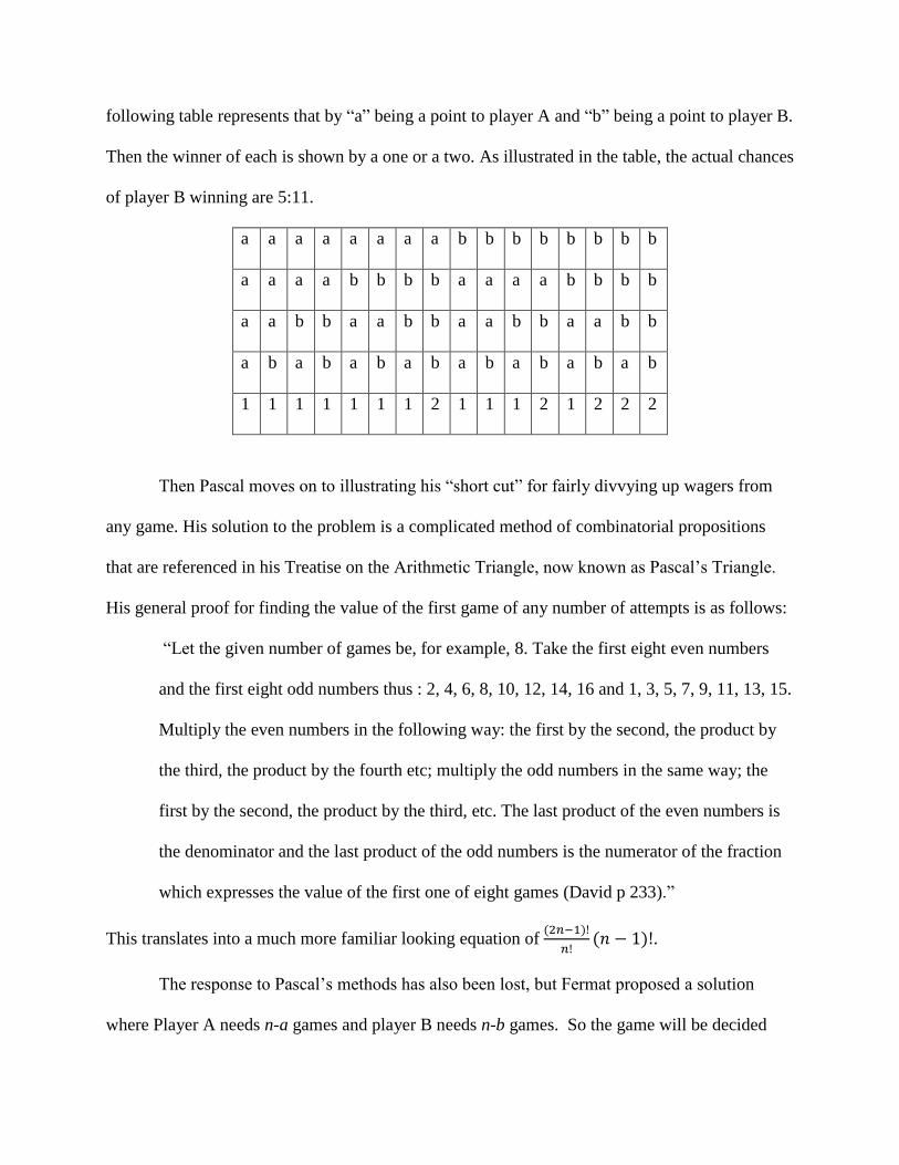
following table represents that by “a” being a point to player A and “b” being a point to player B.

Then the winner of each is shown by a one or a two. As illustrated in the table, the actual chances

of player B winning are 5:11.

a a a a a a a a b b b b b b b b

a a a a b b b b a a a a b b b b

a a b b a a b b a a b b a a b b

a b a b a b a b a b a b a b a b

1 1 1 1 1 1 1 2 1 1 1 2 1 2 2 2

Then Pascal moves on to illustrating his “short cut” for fairly divvying up wagers from

any game. His solution to the problem is a complicated method of combinatorial propositions

that are referenced in his Treatise on the Arithmetic Triangle, now known as Pascal’s Triangle.

His general proof for finding the value of the first game of any number of attempts is as follows:

“Let the given number of games be, for example, 8. Take the first eight even numbers

and the first eight odd numbers thus : 2, 4, 6, 8, 10, 12, 14, 16 and 1, 3, 5, 7, 9, 11, 13, 15.

Multiply the even numbers in the following way: the first by the second, the product by

the third, the product by the fourth etc; multiply the odd numbers in the same way; the

first by the second, the product by the third, etc. The last product of the even numbers is

the denominator and the last product of the odd numbers is the numerator of the fraction

which expresses the value of the first one of eight games (David p 233).”

This translates into a much more familiar looking equation of

.

The response to Pascal’s methods has also been lost, but Fermat proposed a solution

where Player A needs n-a games and player B needs n-b games. So the game will be decided

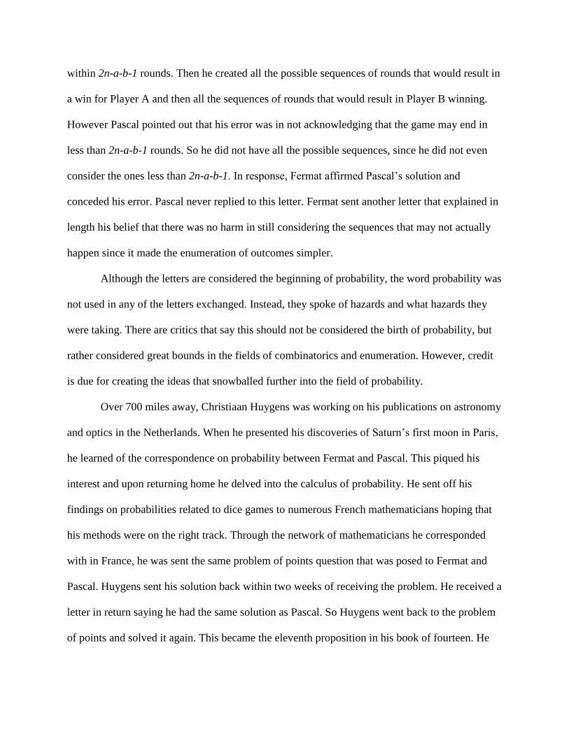
within 2n-a-b-1 rounds. Then he created all the possible sequences of rounds that would result in

a win for Player A and then all the sequences of rounds that would result in Player B winning.

However Pascal pointed out that his error was in not acknowledging that the game may end in

less than 2n-a-b-1 rounds. So he did not have all the possible sequences, since he did not even

consider the ones less than 2n-a-b-1. In response, Fermat affirmed Pascal’s solution and

conceded his error. Pascal never replied to this letter. Fermat sent another letter that explained in

length his belief that there was no harm in still considering the sequences that may not actually

happen since it made the enumeration of outcomes simpler.

Although the letters are considered the beginning of probability, the word probability was

not used in any of the letters exchanged. Instead, they spoke of hazards and what hazards they

were taking. There are critics that say this should not be considered the birth of probability, but

rather considered great bounds in the fields of combinatorics and enumeration. However, credit

is due for creating the ideas that snowballed further into the field of probability.

Over 700 miles away, Christiaan Huygens was working on his publications on astronomy

and optics in the Netherlands. When he presented his discoveries of Saturn’s first moon in Paris,

he learned of the correspondence on probability between Fermat and Pascal. This piqued his

interest and upon returning home he delved into the calculus of probability. He sent off his

findings on probabilities related to dice games to numerous French mathematicians hoping that

his methods were on the right track. Through the network of mathematicians he corresponded

with in France, he was sent the same problem of points question that was posed to Fermat and

Pascal. Huygens sent his solution back within two weeks of receiving the problem. He received a

letter in return saying he had the same solution as Pascal. So Huygens went back to the problem

of points and solved it again. This became the eleventh proposition in his book of fourteen. He

titled the book, De Ratiociniis in Ludo Aleae (Calculations in Games of Chance). It was

published only three years after his initial visit to Paris that started him on his studies. The

fourteen propositions were ground-breaking at this time, although quite different from today’s

knowledge of probability. Still, it was far more comprehensive than the discoveries Fermat and

Pascal had made and was used as the textbook of probability for over 50 years. It wouldn’t be

until Bernoulli published his work, Ars Conjectandi, that the field of probability would change,

but Huygens still holds unchallengeable credit for having hit the tip of the iceberg in the field of

probability.

Jacob Bernoulli, one of the famous Bernoulli brothers, originally attended the University

of Basel in Germany for theology. However, like many mathematicians before him, when he was

18 he became intoxicated with the wonder of math after studying Euclid’s Elements. His focus

was on astronomy, so in the time between when he traveled to study stars, he spent his time

teaching and researching. As a student, he read Huygens’s publication and that sparked his

interest in the subject of probability. Most of his discoveries were in the field of infinite number

theory. So it doesn’t come as a surprise that his theories in probability were heavily tied into

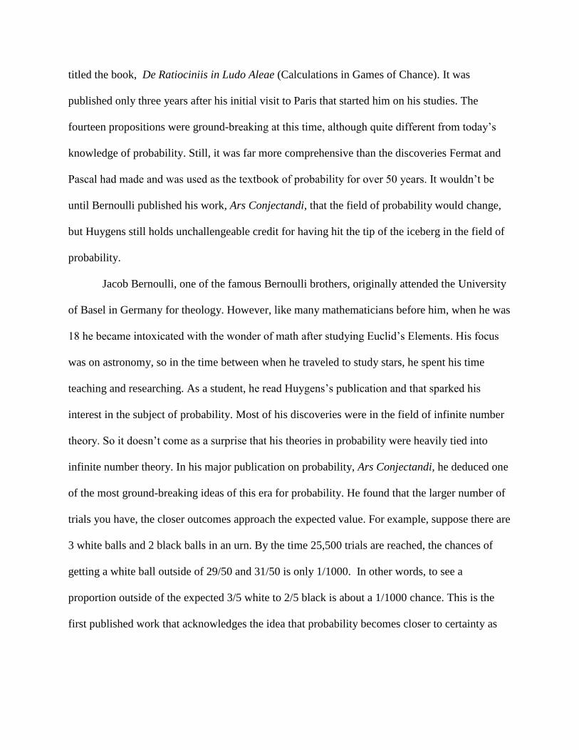
infinite number theory. In his major publication on probability, Ars Conjectandi, he deduced one

of the most ground-breaking ideas of this era for probability. He found that the larger number of

trials you have, the closer outcomes approach the expected value. For example, suppose there are

3 white balls and 2 black balls in an urn. By the time 25,500 trials are reached, the chances of

getting a white ball outside of 29/50 and 31/50 is only 1/1000. In other words, to see a

proportion outside of the expected 3/5 white to 2/5 black is about a 1/1000 chance. This is the

first published work that acknowledges the idea that probability becomes closer to certainty as

the number of trials approaches infinity. He insightfully expanded this idea to the existential

question of fate.

“If thus all events through all eternity could be repeated, by which we would go from

probability to certainty, one would find that everything in the world happens from

definite causes and according to definite rules, and that we would be forced to assume

among the most apparently fortuitous things a certain necessity, or, so to say, FATE

(David p 137).”

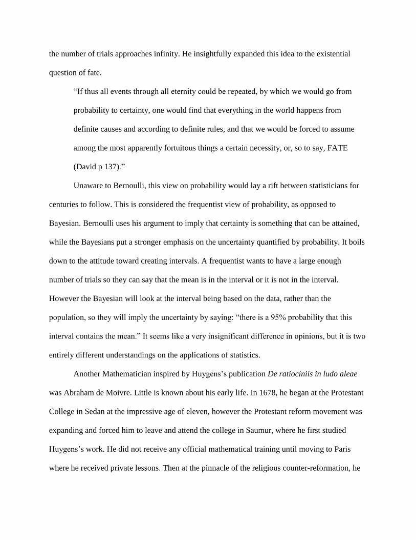
Unaware to Bernoulli, this view on probability would lay a rift between statisticians for

centuries to follow. This is considered the frequentist view of probability, as opposed to

Bayesian. Bernoulli uses his argument to imply that certainty is something that can be attained,

while the Bayesians put a stronger emphasis on the uncertainty quantified by probability. It boils

down to the attitude toward creating intervals. A frequentist wants to have a large enough

number of trials so they can say that the mean is in the interval or it is not in the interval.

However the Bayesian will look at the interval being based on the data, rather than the

population, so they will imply the uncertainty by saying: “there is a 95% probability that this

interval contains the mean.” It seems like a very insignificant difference in opinions, but it is two

entirely different understandings on the applications of statistics.

Another Mathematician inspired by Huygens’s publication De ratiociniis in ludo aleae

was Abraham de Moivre. Little is known about his early life. In 1678, he began at the Protestant

College in Sedan at the impressive age of eleven, however the Protestant reform movement was

expanding and forced him to leave and attend the college in Saumur, where he first studied

Huygens’s work. He did not receive any official mathematical training until moving to Paris

where he received private lessons. Then at the pinnacle of the religious counter-reformation, he

was imprisoned for being a Protestant. It is unclear how long he was detained; some sources say

he was released shortly, while others say he was imprisoned up to almost three years. Regardless,

by the time he was released he was fully versed in the classic works. He traveled to England to

escape the religious turmoil of France. He worked as a tutor and spent his free time, even the

time travelling from pupil to pupil, studying any mathematical work he could get his hands on

and networking with English mathematicians. Also at this time, he began to go to a coffee house

after his work tutoring, where he would charge gamblers for calculating their odds. In 1718 he

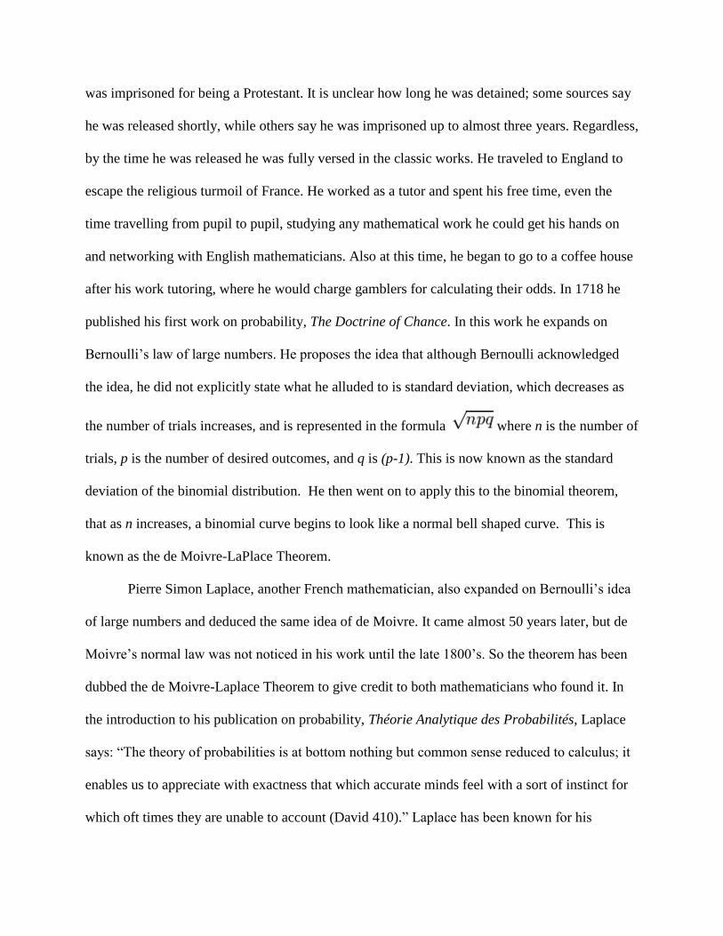
published his first work on probability, The Doctrine of Chance. In this work he expands on

Bernoulli’s law of large numbers. He proposes the idea that although Bernoulli acknowledged

the idea, he did not explicitly state what he alluded to is standard deviation, which decreases as

the number of trials increases, and is represented in the formula where n is the number of

trials, p is the number of desired outcomes, and q is (p-1). This is now known as the standard

deviation of the binomial distribution. He then went on to apply this to the binomial theorem,

that as n increases, a binomial curve begins to look like a normal bell shaped curve. This is

known as the de Moivre-LaPlace Theorem.

Pierre Simon Laplace, another French mathematician, also expanded on Bernoulli’s idea

of large numbers and deduced the same idea of de Moivre. It came almost 50 years later, but de

Moivre’s normal law was not noticed in his work until the late 1800’s. So the theorem has been

dubbed the de Moivre-Laplace Theorem to give credit to both mathematicians who found it. In

the introduction to his publication on probability, Théorie Analytique des Probabilités, Laplace

says: “The theory of probabilities is at bottom nothing but common sense reduced to calculus; it

enables us to appreciate with exactness that which accurate minds feel with a sort of instinct for

which oft times they are unable to account (David 410).” Laplace has been known for his

inductive reasoning in probability, which typical of Bayesian probability, was very ground-

breaking for this time. With his outstanding reasoning abilities, he developed the method of least

squares; however he did not publish it with any relation to probability. Laplace is the last of the

mathematicians to make great bounds in the field of probability during this time period in

France. It is the close of an intellectual era that was the perfect climate for mathematical

networking, building off of one another’s ideas and findings.

The history of probability theory could go on infinitely to cover more mathematicians

before and during that time, and the mathematicians still making progress today. There are

numerous mathematicians of the current era that made bounds in the field but the ones discussed

previously are given the most glory for establishing the ideas that mathematicians would draw on

for centuries. They may not have been totally accurate, but they were the first to quantify the

random events of life. What was previously referred to as righteous intervention from God had

been discovered to be relatively predictable events.

Works Cited

Abrams, Bill. "A Brief History of Probability." Second Moment, 2003. Web. 07 Dec. 2012.

Annis, Charles, PE. "Frequentists and Bayesians." Frequentists and Bayesians. N.p., 15 Jan.

2012. Web. 07 Dec. 2012.

Apostal, Tom M. "A Short History of Probability." Caclulus. 2nd ed. Vol. 2. N.p.: John Wiley &

Sons, 1969. N. pag. A Short History of Probability. Web. 07 Dec. 2012.

David, F. N. Games, Gods and Gambling: The Origins and History of Probability and Statistical

Ideas from the Earliest times to the Newtonian Era. New York: Hafner Pub., 1962. Print.

Devlin, Keith J. The Unfinished Game: Pascal, Fermat, and the Seventeenth-century Letter That

Made the World Modern. New York: Basic, 2008. Print.

O'Connor, J. J., and E. F. Robertson. "Blaise Pascal." Pascal Biography. N.p., n.d. Web. 07 Dec.

2012.

"Sources in the History of Probability and Statistics." Sources in the History of Probability and

Statistics. Xavier University, n.d. Web. 07 Dec. 2012.

JAMES STIRLIn!G An!D N !UMBERS OF THE FIRST An!D SECOn!D

KIn!D

MATT JOHA(N !2)

Many know James Stirling as a British architect who built the Florey Building at Oxford

University in 1971. The James Stirling to be considered is not an architect, but a mathe-

matician who studied at Oxford University in 1711. The mathematician James Stirling has

an important role in some breakthrough periods for mathematics. He lived an interesting

life, meeting people such as Isaac Newton and Nicolaus Bernoulli I. Stirling solved many

mathematical questions in his lifetime and published some very important works.

Stirling‘s mother and father were Archibald Stirling and Archibald‘s second wife, Anna

Hamilton. Archibald and Anna had James in May of 1692 in Garden, Scotland. James

was born into a very supportive family to the Jacobite cause. Many did not agree with

the supporters of the Jacobite cause and this showed starting at the age of 17. Stirlings

father, Archibald, was arrested after accusations of high treason because of his Jacobite

support. [1] Jacobitism is the movement in Great Britain and Ireland between 1688 and

1746 to restore power to King James II of England. [2]

Not much is known about Stirling‘s younger years. The first known information about

Stirling is that he traveled to Oxford in the fall of 1710. [1] He went to Oxford to matriculate

at a University. Matriculate comes from the Latin word matricula, or “little list.” [3] In

January of 1711, Stirling‘s plan came true when he matriculated at Balliol College Oxford.

There is no certainty, but it is said that Stirling also studied at the University of Glasgow.

[1]

Date: December 13, 2012.

1

2 MATT JOHA(N !2)

Stirling was awarded a scholarship in 1711 with only one rule, to swear an oath when

matriculating. His Jacobite sympathies would not let him do so, but he was excused. In

1715, there was a Jacobite rebellion, which created a problem for Stirling. Stirling was

withdrawn from his excuse to not swear on the oath. Upon refusal of swearing on the

oath, Stirling lost all of his scholarships and could not graduate from Oxford. [1] Stirling‘s

support for the Jacobites now hindered his life in the biggest way possible.

Stirling may have bounced around in Oxford for a while, but that ended when he left

for Italy.[4] While in Italy Stirling almost became a professor of mathematics in Venice,

but for unknown reasons this did not happen. All was not lost, however. In 1717, while in

Italy, Stirling published his first work.

The work titled Lineae Tertii Ordinis Neutonianae extends ideas of other mathemati-

cians. There are results on the curve of quickest descent, the catenary and orthogonal

trajectories. The problem of orthogonal trajectories was first raised by Gottfried Wil-

helm Leibniz. [1] Stirling is known to be the mathematician who solved the problem in

1716. Some other famous mathematicians working on the problem as well include Johann

Bernoulli, Nicolaus Bernoulli I, Nicolaus Bernoulli II and Leonard Euler.

In 1718, Stirling published more work, this time through Newton a paper titled Methodus

Differentialis Newtoniana Illustrata or the Illustrated Newtonian Differential Method in

English.[4] In 1719, Stirling decided to submit this to the Royal Society of London from

Venice. The paper was received and reported to their meeting on June 18th of the year.

The years from 1716 to 1719 had been a busy time for Stirling, but it seems that he would

not slow down. In 1721 Stirling was in Padua where he took classes under the chair of the

great Nicolaus Bernoulli II. It wasnt long before Stirling returned to Glasgow. This was

at a similar time when Nicolaus Bernoulli II left Padua. [1] In 1722, Stirling left with the

intentions of becoming a teacher in London.

In 1724 Stirling travelled to London. He stayed in London for 10 years and was very

active in the mathematics world. Stirling corresponded with many mathematicians and

JAMES STIRLIn!G An!D N !UMBERS OF THE FIRST An!D SECOn!D KIn!D 3

had a good friendship with Isaac Newton. Newton proposed Stirling to the Royal Society

of London for his work. In 1726 Stirling was elected for the society. Things were going well

for Stirling at this time and in 1727 he reached his goal and became a teacher at William

Watts Academy on Little Tower Street, London. [1]

The year 1730 proved to be Stirling‘s most important, this was the year that Stirling

published the Methodus Differentialis. The title is translated in English to mean “The

Method of Differences.” In this book is treatise on infinite series, summation, interpolation

and quadrature. Also in this book is the asymptotic formula for n!, which made Stirling

famous and why he is relevant today. It was Proposition 28, example 2 of Methodus Dif-

ferentialis that approximated n!. The approximation is n! ≈√

2πn(ne )n and appropriately

so called the Stirling approximation.[5] Abraham de Moivre also published Miscellanea

Analytica in 1730 deriving the series expansion formula. [1][5] Stirling wrote de Moivre a

letter pointing out the errors that he had made.

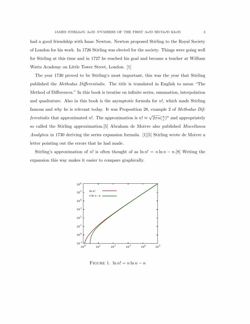
Stirling’s approximation of n! is often thought of as lnn! = n lnn − n.[8] Writing the

expansion this way makes it easier to compare graphically.

Figure 1. lnn! = n lnn− n

4 MATT JOHA(N !2)

The graph of lnn! and n lnn−n shows that Stirling’s approximation of n! is acceptable.

The approximation does show pretty poor comparisons, but as n increases the two converge

closer and closer.

In Methodus Differentialis Stirling expands on the Newton series. A Newton series is

denoted as P0(z) = 1, P1(z) = z, P2(z) = z(z − 1), P3(z) = z(z − 1)(z − 2), · · · , Pk(z) =

z(z − 1) · · · (z − k + 1). The Newton series can also be written as,

f(z) =∞∑k=0

akz(z − 1)(z − 2) · · · (z − k + 1)

= a0 + a1z + a2z(z − 1) + a3z(z − 1)(z − 2) + · · ·

[4].

At the beginning of his book Stirling studied the coefficients Amn in

zm = Am1 z +Am

2 z(z − 1) +Am3 z(z − 1)(z − 2) + · · ·+Am

n z(z − 1) · · · (z −m+ 1)

.

Stirling obtained the following for Amn :

z = z

z2 = z + z(z − 1)

z3 = z + 3z(z − 1) + z(z − 1)(z − 2)

z4 = z + 7z(z − 1) + 6z(z − 1)(z − 2) + z(z − 1)(z − 2)(z − 3)

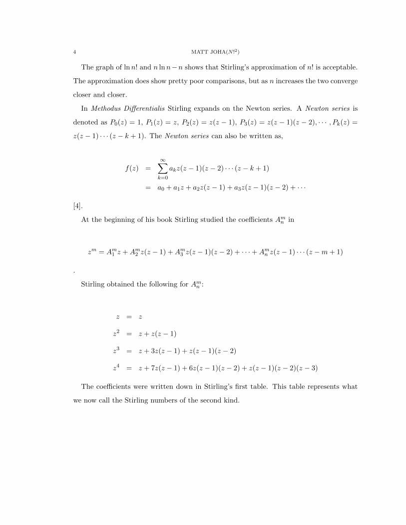
The coefficients were written down in Stirling’s first table. This table represents what

we now call the Stirling numbers of the second kind.

JAMES STIRLIn!G An!D N !UMBERS OF THE FIRST An!D SECOn!D KIn!D 5

Figure 2. Stirling Numbers of the Second Kind

The Stirling numbers of the second kind are denoted as S(n, k) or

nk. The Stirling

numbers of the second kind are the number of ways to partition a set of n objects into k

non-empty subsets. [4] A good way to think about creating these partitions is by having

number of sweaters be n and having number of boxes be k. It is the summer and one looks

to put the sweaters away into boxes. The sweaters must all go into a box, but no box may

be left empty. If one has 3 sweaters and 3 boxes, there is only one way to put the sweaters

into boxes and that is to put one sweater in each box. Similarly, if there are 3 sweaters

but only 1 box to put them in, there is only one way to put them into boxes. There is only

one way to put them into the boxes and that is to dump all 3 sweaters into the one box.

If one has 3 sweaters and only 2 boxes to put them into is where partitioning gets fun.

There are three sweaters, one of which is green, another that is purple and another that

is red. Now the green and red sweater can be in separate boxes. Then either the purple

sweater is in the box with the green sweater or in the box with the red sweater. If the

green sweater and purple sweater were our starting sweaters in separate boxes, then the

red sweater can either go in the box with the green one or in the box with the purple one.

Notice that there had already been a box that was accounted for with a purple sweater

6 MATT JOHA(N !2)

and red sweater. There are no more ways to do this and there are only three ways to put

these three sweaters into 2 boxes. [7]

Notice, from the Stirling chart, the Stirling number S(3, 1) = 1 and the Stirling numbers

S(3, 2) = 3 and S(3, 3) = 1. Looking ahead on Stirling’s table one can say that there are

7770 ways to put 9 sweaters into 4 boxes (S(9, 4)). While the Stirling numbers of the

second kind originally came from coefficients of the Newton series of zk, there are many

helpful uses of these numbers and why the Stirling numbers are still interesting to study

today.

Also in Stirling’s Methodus Differentialis is Stirling’s study on interpolation. In par-

ticular, Stirling studied the sequence Tn+1 = nTn with T1 = 1. The numbers are as

follows:

T1 = 1 = 1

T2 = 1(1) = 1

T3 = 2(1) = 2

T4 = 3(2) = 6

T5 = 4(6) = 24

T6 = 5(24) = 120

T7 = 6(120) = 720

T8 = 7(720) = 5040

These numbers are the start of what are now known as the Stirling numbers of the first

kind. The Stirling numbers of the first kind are denoted as s(n, k) or

nk

. The Stirling

numbers of the first kind are known as the number of permutations of n elements with k

disjoint cycles.[4]

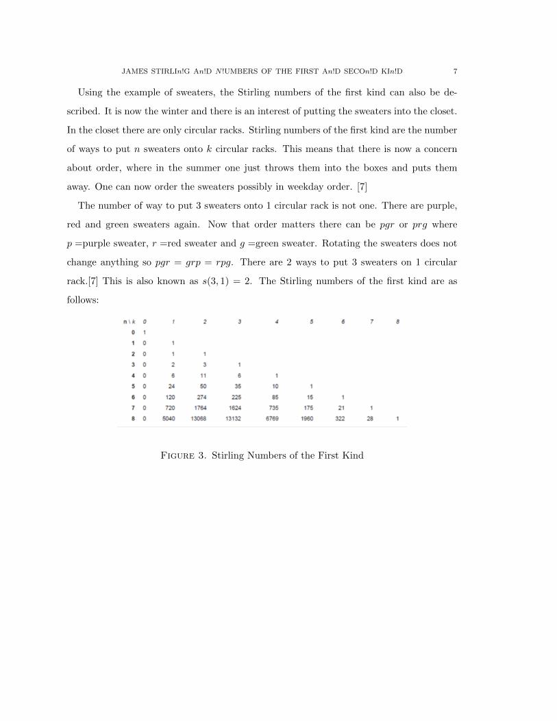
JAMES STIRLIn!G An!D N !UMBERS OF THE FIRST An!D SECOn!D KIn!D 7

Using the example of sweaters, the Stirling numbers of the first kind can also be de-

scribed. It is now the winter and there is an interest of putting the sweaters into the closet.

In the closet there are only circular racks. Stirling numbers of the first kind are the number

of ways to put n sweaters onto k circular racks. This means that there is now a concern

about order, where in the summer one just throws them into the boxes and puts them

away. One can now order the sweaters possibly in weekday order. [7]

The number of way to put 3 sweaters onto 1 circular rack is not one. There are purple,

red and green sweaters again. Now that order matters there can be pgr or prg where

p =purple sweater, r =red sweater and g =green sweater. Rotating the sweaters does not

change anything so pgr = grp = rpg. There are 2 ways to put 3 sweaters on 1 circular

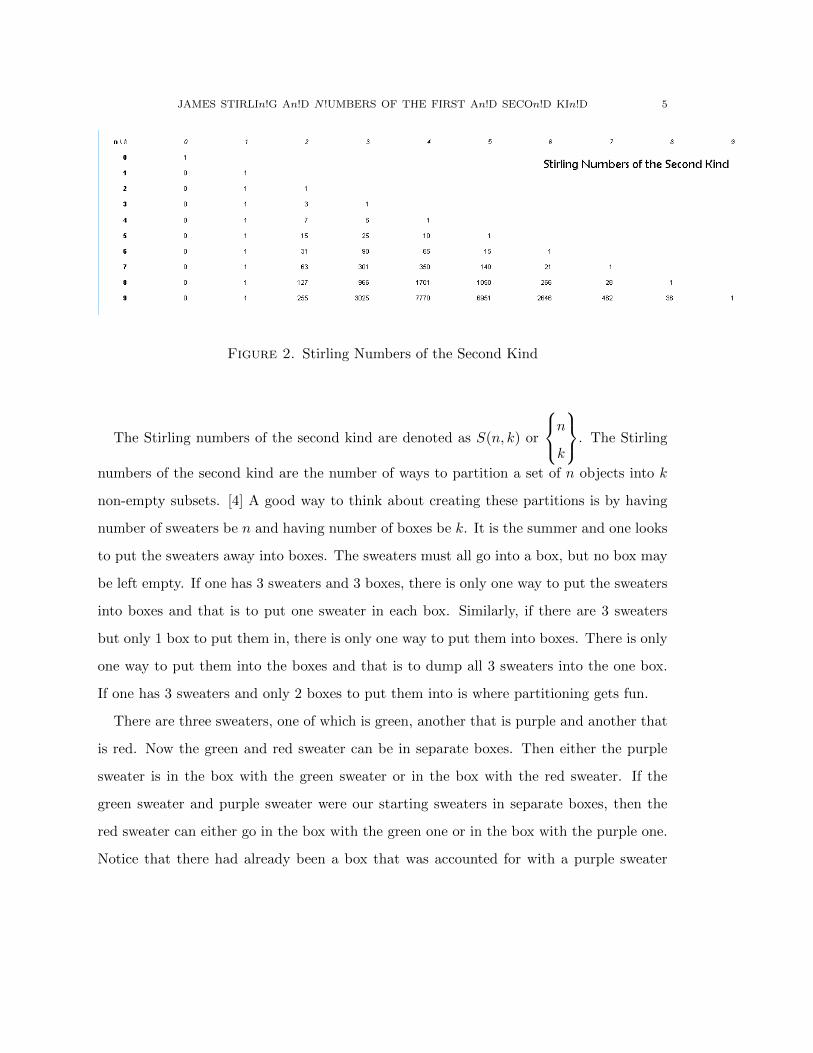
rack.[7] This is also known as s(3, 1) = 2. The Stirling numbers of the first kind are as

follows:

Figure 3. Stirling Numbers of the First Kind

8 MATT JOHA(N !2)

Stirling’s series of Tn+1 became known to be the Stirling number of the first kind when

k = 1. The formula s(n + 1, k) = s(n, k − 1) − ns(n, k) helps understand the rest of the

table.

Stirling published some great work in 1730 and the work did not go unnoticed. In 1736

Leonard Euler wrote Stirling a letter. The great Euler was impressed with what Stirling

had published and wanted to learn more. Stirling was extremely busy at this time in his

life and took two years to respond to the letter. In Stirling’s response, he said that he

would put Euler’s name forward for election to the Royal Society, but never got around to

actually doing so. Euler was proposed, by many mathematicians that were not Stirling, to

the Royal Society in 1746.

Stirling was not done publishing work in 1745. He published a paper on the ventilation

of mine shafts. There was a major rebellion of the Jacobite cause in this year. In 1746 the

chair of Edinburgh had died and Stirling was considered to be the new chair. Stirling’s

strong support for the Jacobite cause made it impossible for him to get the chair. Stirling

was elected as a member of the Royal Society of Berlin in 1746. It only took seven years

for Stirling to resign because he could no longer afford the subscriptions.

James Stirling was not an architect, but a very good mathematician. He was associated

with names such as Newton, Bernoulli, and Euler, who thought that he was very intelligent.

Being a big supporter of the Jacobite cause held him back in multiple ways throughout his

life. Even with distractions and hatred Stirling was able to publish many papers, and we

are still interested in his work centuries later. It is interesting that his name is not used

more often and more well-known. This could be because of his support for the Jacobite

cause holding him back from a lot in his life. Stirling died in December of 1770 and his

work is still studied today. Supporter of the Jacobite cause or not, he did some great

things.

JAMES STIRLIn!G An!D N !UMBERS OF THE FIRST An!D SECOn!D KIn!D 9

References

[1] “James Stirling.” Stirling Biography. The MacTutor History of Mathematics archive, n.d. Web. 5 Dec.

2012, http://www-history.mcs.st-and.ac.uk/Mathematicians/Stirling.html

[2] The Jacobites, Britain and Europe 16881788, Daniel Szechi, Manchester University Press 1994

[3] “Matriculate.” Merriam-Webster. Merriam-Webster, n.d. Web. 5 Dec. 2012, http://www.merriam-

webster.com/dictionary/matriculate

[4] Boyadzhiev, Khristo N. “Close Encounters with the Stirling Numbers of the Second Kind.” Mathe-

matics Magazine 85.4(2012): 252-66. Print.

[5] Gale, Thomas. “James Stirling Biography.” BookRags. BookRags, n.s. Web. 5 Dec. 2012.

[6] Milson, Robert. “Stirling numbers of the first kind” (version 3). PlanetMath.org,

http://planetmath.org/encyclopedia/StirlingNumbers.html

[7] Stenson, C. (2012, October). Stirling Numbers. Speech presented at Juniata College, Huntingdon, PA.

[8] Schroeder, Daniel V., An Introduction to Thermal Physics, Addison Wesley, 2000,

http://hyperphysics.phy-astr.gsu.edu/hbase/math/stirling.html

Seven Bridges of Königsberg: An Eulerian Path Johnson 1

During the time of the nomads of the earliest century of man, mathematics had no presence in

the world. As these prehistoric men settled during the Neolithic period, the need for mathematics began

to grow. Counting livestock and measuring areas of fields developed into the two major branches of

mathematics: arithmetic and geometry, respectively (Dunham). As the years progressed, so too did the

field of mathematics. The importance of mathematics in society grew as society and mathematics itself

grew more complex. Many fields of mathematics were born to satisfy a particular need of society,

usually to make daily life easier for the people. Fascinatingly, however, mathematics did not always

originate from a search to alleviate mankind’s struggle. Graph theory, which is now known as a

subdivision of combinatorics, had a humble, almost silly beginning. Leonhard Euler, renowned for his

work with infinitesimal calculus and other fields of mathematics and physics and remembered by the

many equations, functions, and theorems that bear his name, discovered the field of graph theory when

he published his work about a puzzle in 1736. This publication, The Solution of a Problem Relating to the

Geometry of Position, laid the groundwork for graph theory, a field of mathematics that would

eventually make major contributions in the fields of physics, chemistry, biology, linguistics, computer

science, and many more, by examining the well-known puzzle known as the seven bridges of

Königsberg.

Leonhard Euler’s lifelong dedication to the sciences and, in particular, mathematics eventually

led to his founding of graph theory. Euler was born on April 15, 1707, in Basel, Switzerland. His father,

Paul Euler, was a Protestant minister who taught Leonhard mathematics at a very young age. Even

though the school Euler attended when he was young was very poor and lacked a mathematical

curriculum, he still managed to tame the passion for mathematics he learned from his father with

mathematical readings on his own time. At age 14, Euler was sent to attend school at the University of

Basel to prepare for the ministry. It did not take long for his potential in mathematics to be noticed by

Seven Bridges of Königsberg: An Eulerian Path Johnson 2

the very famous Johann Bernoulli, a professor at the university. Euler would have a longstanding

relationship with the Bernoulli family for the rest of his life. It is Johann Bernoulli who persuaded Euler’s

father to allow young Leonhard to change his area of study from theology to mathematics. Once on the

mathematical path, Euler began to excel in the field. By the time he completed his studies in 1726 at the

age of 19, he had a paper in print, a second place finish in the grand prize competition in the Paris

Academy, and a job offer for a professorship at the St. Petersburg Academy of Sciences in Russia. He

took the job in 1727 and quickly became the senior chair of the mathematics department in 1733, at the

age of 26. From that time until his death on September 18, 1783, Euler established himself as “the most

prolific writer of mathematics of all time” (O’Connor). Of those writings, a particular article of interest,

Solutio problematis ad geometriam situs pertinentis (The Solution of a Problem Relating to the Geometry

of Position), was written on a puzzle developed by the people of a city in Eastern Prussia and was the

building blocks for the field of graph theory. (O’Connor)

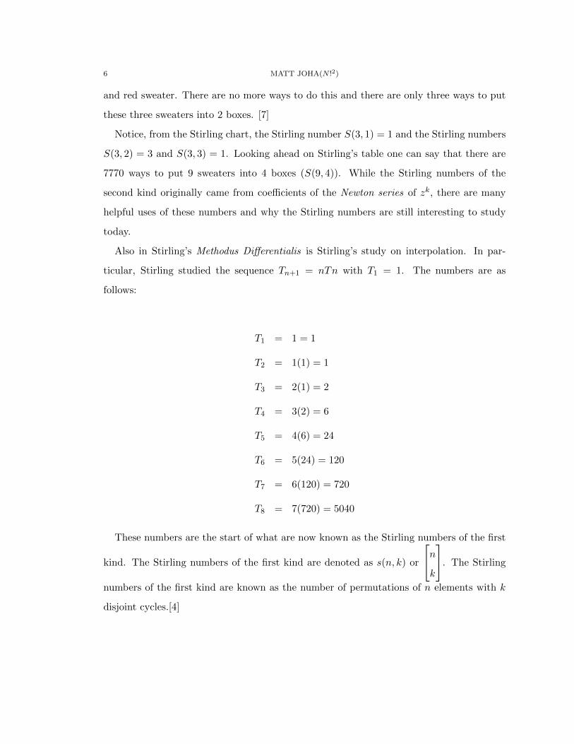
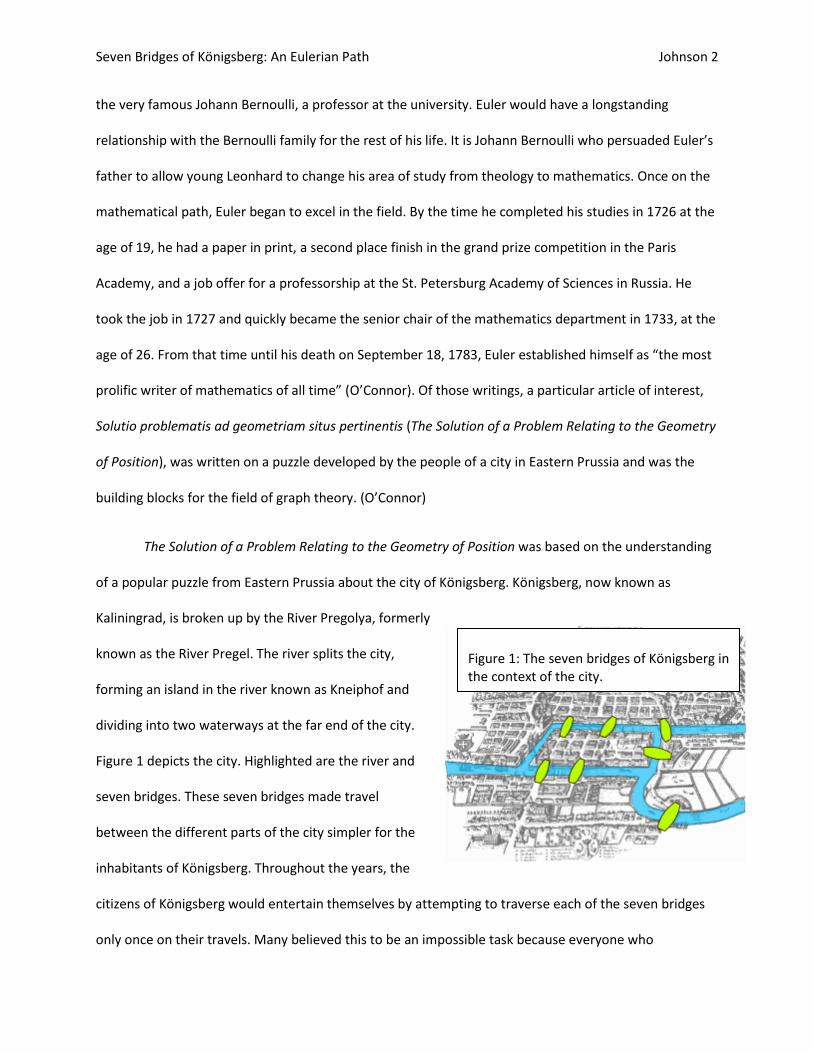
The Solution of a Problem Relating to the Geometry of Position was based on the understanding

of a popular puzzle from Eastern Prussia about the city of Königsberg. Königsberg, now known as

Kaliningrad, is broken up by the River Pregolya, formerly

known as the River Pregel. The river splits the city,

forming an island in the river known as Kneiphof and

dividing into two waterways at the far end of the city.

Figure 1 depicts the city. Highlighted are the river and

seven bridges. These seven bridges made travel

between the different parts of the city simpler for the

inhabitants of Königsberg. Throughout the years, the

citizens of Königsberg would entertain themselves by attempting to traverse each of the seven bridges

only once on their travels. Many believed this to be an impossible task because everyone who

Figure 1: The seven bridges of Königsberg in the context of the city.

Seven Bridges of Königsberg: An Eulerian Path Johnson 3

attempted failed; however, there was no explanation as to why this was not an accomplishable feat. In

1736, a 29-year old Euler decided to look at this puzzle in more detail, and he published his paper on the

subject. (Biggs 1-2)

In the opening paragraph of his paper, Euler acknowledges that the problem of the seven

bridges of Königsberg is of a branch of geometry that receives little attention: the geometry of positions.

He mentions that Leibniz first mentioned this branch of geometry that is overshadowed by the

geometry concerned with magnitudes. Euler explains that geometry of positions is special because it “is

concerned only with the determination of position and its properties” (Biggs 3) and not with calculations

or measurements. Geometry of position, as described by Euler, evolved into what is now known as

graph theory. As a result, Euler’s paper is known as the first paper to have been written on graph theory.

Euler was looking for geometry of position problems to analyze because “it had not yet been

satisfactorily determined what kind of problems [were] relevant to this geometry of position, or what

methods should be used in solving them” (Biggs 3). He found the problem he was looking for in the

seven bridges of Königsberg puzzle because its solution concerned no calculations or measurements,

only position. The aim of his paper was to describe the rules and methods necessary for solving this

problem and others like it. (Biggs 3)

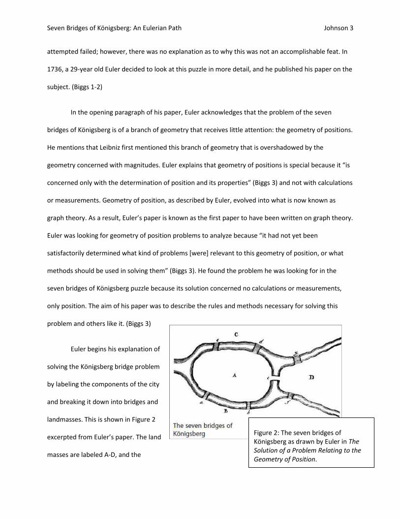
Euler begins his explanation of

solving the Königsberg bridge problem

by labeling the components of the city

and breaking it down into bridges and

landmasses. This is shown in Figure 2

excerpted from Euler’s paper. The land

masses are labeled A-D, and the

Figure 2: The seven bridges of Königsberg as drawn by Euler in The Solution of a Problem Relating to the Geometry of Position.

Seven Bridges of Königsberg: An Eulerian Path Johnson 4

bridges are labeled a-g. Because Euler wishes to devise a solution for any problem involving a number of

landmasses and bridges, he denies the usefulness of a guess-and-check method of tracing paths until

one is found or all paths are exhausted. Instead, Euler reasons that he is to find a way in which A-D can

be arranged so that each bridge between two landmasses is crossed only once. He shows that for this

particular problem, it will be an eight letter arrangement because between each landmass, AB for

example, lays one bridge. Since seven bridges must be crossed, eight letters must be used in total to

represent the crosses. Moreover, the total number of times someone can traverse an area (A, B, C, or D)

is equal to eight. However, he decides that it is best he finds a rule for finding whether or not an

arrangement can exist before finding what the particular arrangement is. (Biggs 4)

In order to find a rule, Euler considers one area with a number of bridges leading to it. He shows

that if one bridge leads to the area, the area will be traveled only once. If three bridges lead into the

area, no matter where the person starts, the area will be traveled twice. If there are five bridges, the

area will be traversed thrice and so on. Therefore, Euler reasons that if the number of bridges is any odd

number, that number increased by 1 then half is the number of times the area is entered. When he

applied this to the seven bridges problem, he discovered that A is entered thrice, and B, C, and D are

entered twice each. Since these areas in whole are traveled nine times (represented by nine letters),

the seven bridges problem is not possible since he showed earlier that for each bridge to be crossed

only once, the total number of area visits had to equal eight. Euler then expands his rule to include an

even number of bridges by the same thought process. If two bridges lead to an area, the area can be

traversed either once or twice: once if the journey is not started in the area, twice if the journey is

started in the area. In the case of four bridges leading to an area, if the journey does not start in the

area, the area is traversed twice, and if the journey begins in the area, the area is traversed thrice and so

on. Therefore, Euler reasons that if the number of bridges is even, than the number of times an area is

traversed is equal to half the number of bridges if the journey does not start in the area and it is equal to

Seven Bridges of Königsberg: An Eulerian Path Johnson 5

half the number of bridges plus one if the journey begins in the area. With the new rules, Euler devises a

method for solving such problems as the seven bridges problem. (Biggs 4-5)

In solving a problem involving areas separated by bridges, Euler lays out a simple method for

finding whether or not a path can be found that travels each and every bridge only once. First, he labels

the areas with capital letters. Then he takes the total number of bridges and adds one. This number is

utilized later. Next he writes the areas in a column and notes the number of bridges leading to each in

another column. Then he indicates those areas with an even number of bridges leading to it with an

asterisk. Next to the even numbers, he writes half of the number. Next to the odd numbers, he increases

the number by one and then halves it. He sums this last column and compares it to the number found at

the beginning of the process. If the sum of this column is greater than the number of bridges plus one,

the journey is impossible. If the sum is one less or equal to the number of bridges plus one, the journey

is possible given that if the sum is equal, the journey begins from an area with an odd number of bridges

and if the sum is one less, the journey begins from an area with an even number of bridges. Euler applies

this process to Königsberg, and again the result was that it is impossible to travel across the bridges only

once in a single journey. After showing this, he goes through the method again with fifteen bridges and

six lands. This example was included to show an instance where it was possible to traverse all the

bridges only once in a single journey. He concludes his paper by summing his findings. (Biggs 6)

In the years after Euler’s paper, the graph theory field he started grew exponentially and

modern graph theory developed Euler’s method of solving the seven bridges of Königsberg into Eulerian

path problems. In modern graph theory, an Eulerian path is a path which contains each edge of a graph

only once in a sequence of edges and vertices. A graph consists of a finite set of vertices and a finite set

of edges (Biggs 9). In comparison to Euler’s paper on the subject, not much has changed other than the

wording. An Eulerian path is a seven bridges of Königsberg problem. The edges are the bridges and the

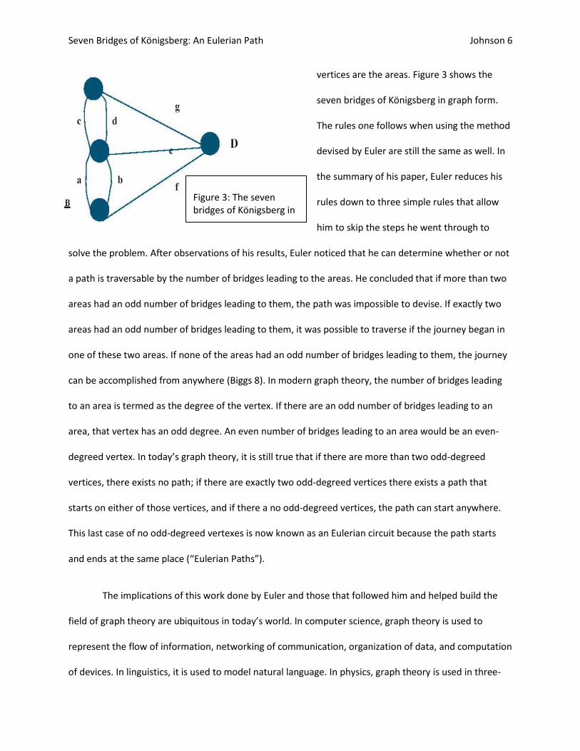
Seven Bridges of Königsberg: An Eulerian Path Johnson 6

vertices are the areas. Figure 3 shows the

seven bridges of Königsberg in graph form.

The rules one follows when using the method

devised by Euler are still the same as well. In

the summary of his paper, Euler reduces his

rules down to three simple rules that allow

him to skip the steps he went through to

solve the problem. After observations of his results, Euler noticed that he can determine whether or not

a path is traversable by the number of bridges leading to the areas. He concluded that if more than two

areas had an odd number of bridges leading to them, the path was impossible to devise. If exactly two

areas had an odd number of bridges leading to them, it was possible to traverse if the journey began in

one of these two areas. If none of the areas had an odd number of bridges leading to them, the journey

can be accomplished from anywhere (Biggs 8). In modern graph theory, the number of bridges leading

to an area is termed as the degree of the vertex. If there are an odd number of bridges leading to an

area, that vertex has an odd degree. An even number of bridges leading to an area would be an even-

degreed vertex. In today’s graph theory, it is still true that if there are more than two odd-degreed

vertices, there exists no path; if there are exactly two odd-degreed vertices there exists a path that

starts on either of those vertices, and if there a no odd-degreed vertices, the path can start anywhere.

This last case of no odd-degreed vertexes is now known as an Eulerian circuit because the path starts

and ends at the same place (“Eulerian Paths”).

The implications of this work done by Euler and those that followed him and helped build the

field of graph theory are ubiquitous in today’s world. In computer science, graph theory is used to

represent the flow of information, networking of communication, organization of data, and computation

of devices. In linguistics, it is used to model natural language. In physics, graph theory is used in three-

Figure 3: The seven bridges of Königsberg in graph form.

Seven Bridges of Königsberg: An Eulerian Path Johnson 7

dimensional modeling of complicated atom structures. In biology, Eulerian paths are used to describe

the migration habits of animals, where the area of habitat is represented by a vertex and the migration

paths are represented by edges. The list of practical uses of graph theory continues on and without the

contributions of Euler, who knows if these processes used every day in a myriad of fields would be as far

along as they are today. (“Graph Theory”)

Using the seven bridges of Königsberg puzzle, Euler, in The Solution of a Problem Relating to the

Geometry of Position, was able to derive a solution to the first problem to ever to be written about in

graph theory. The work that he revealed in the paper has stood the test of time and is now the most

basic of concepts for the field of graph theory. The humble origins of graph theory, like the humble

origins of Euler, laid the groundwork for importance in the field of mathematics. Although it was not

developed to ease the lives of the average citizen, Euler’s paper, as well as the resulting field of

mathematics, has certainly left an impact on the world we live in today.

Seven Bridges of Königsberg: An Eulerian Path Johnson 8

Works Cited

Biggs, Norman, Edward Keith. Lloyd, Robin James. Wilson, and Leonhard Euler. "Paths." Graph theory 1736-1936. Oxford: Oxford UP, 1977. 1-9. This book was written as a textbook for those learning graph theory. The authors did this by including original sources of those influential on the topic. For use in this paper, the focus was on the excerpted source of Euler on the geometry of position. When used for citation in the paper, sometimes it is unclear whether it is from the author's of the text or from Euler himself. However, Euler is addressed in the paragraphs in which his work is cited from this work.

Dunham, William. "Hippocrates' Quadtrature of the Lune." Journey through genius: The great theorems of mathematics. New York: Penguin Books, 1991. 1-2.

"Eulerian path." Wikipedia. 14 Nov. 2012. Wikimedia Foundation. 28 Nov. 2012 <http://en.wikipedia.org/wiki/Eulerian_path>.

"Graph theory." Wikipedia. 12 Apr. 2012. Wikimedia Foundation. 28 Nov. 2012 <http://en.wikipedia.org/wiki/Graph_theory>.

O'Connor, J. J., and E. F. Robertson. "Leonhard Euler." Euler biography. Sept. 1998. University of St. Andrews, Scotland. 28 Nov. 2012 <http://www-history.mcs.st-and.ac.uk/Biographies/Euler.html>.

Lloyd Shapley and His Work on Game Theory

Stephen Kidhardt

History of Mathematics

Juniata College

December 12, 2012

Economics is the study of the way societies use and allocate their resources. When

being studied and analyzed, the price system is what generally contributes to how these

resources are allocated. What happens when prices cannot be the root cause for either

legal or ethical reasons, or when prices cause an unstable and crowded market that does

not run efficiently and effectively? These are the questions the most recent recipients of

the Noble Prize for economics sought to answer. Alvin Roth and Lloyd Shapley produced

algorithms and real-life evidence showing a much more effective way to allocate resources

in these markets. Their work was in the forefront in market design and stable allocations

with the use of cooperative game theory.

Game theory has become a branch of economics where mathematical models are

used for the study of conflict and cooperation between intelligent and rational people.

Many different fields then branched off of game theory including symmetric games,

infinitely long games, and differential games just to name a few. Shapley and Roth used

cooperative game theory for finding stable allocations in markets. Cooperative game

theory assumes that players are able to form binding commitments with each other as well

as being able to communicate with each other. John Forbes Nash’s work in this subject

resulted in an equilibrium which was named after him. This equilibrium states that if each

player chooses a strategy and no other player can benefit by changing their solution, while

the other player’s solutions remain unchanged, then the situation is called a Nash

Equilibrium. A simple example of this involves the prisoner’s dilemma. Each player has the

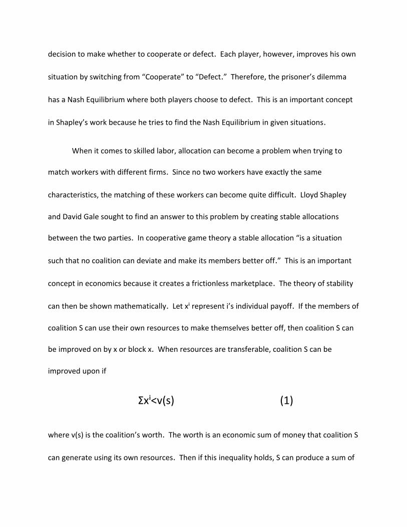
decision to make whether to cooperate or defect. Each player, however, improves his own

situation by switching from “Cooperate” to “Defect.” Therefore, the prisoner’s dilemma

has a Nash Equilibrium where both players choose to defect. This is an important concept

in Shapley’s work because he tries to find the Nash Equilibrium in given situations.

When it comes to skilled labor, allocation can become a problem when trying to

match workers with different firms. Since no two workers have exactly the same

characteristics, the matching of these workers can become quite difficult. Lloyd Shapley

and David Gale sought to find an answer to this problem by creating stable allocations

between the two parties. In cooperative game theory a stable allocation “is a situation

such that no coalition can deviate and make its members better off.” This is an important

concept in economics because it creates a frictionless marketplace. The theory of stability

can then be shown mathematically. Let xⁱ represent i’s individual payoff. If the members of

coalition S can use their own resources to make themselves better off, then coalition S can

be improved on by x or block x. When resources are transferable, coalition S can be

improved upon if

Σxⁱ<v(s) (1)

where v(s) is the coalition’s worth. The worth is an economic sum of money that coalition S

can generate using its own resources. Then if this inequality holds, S can produce a sum of

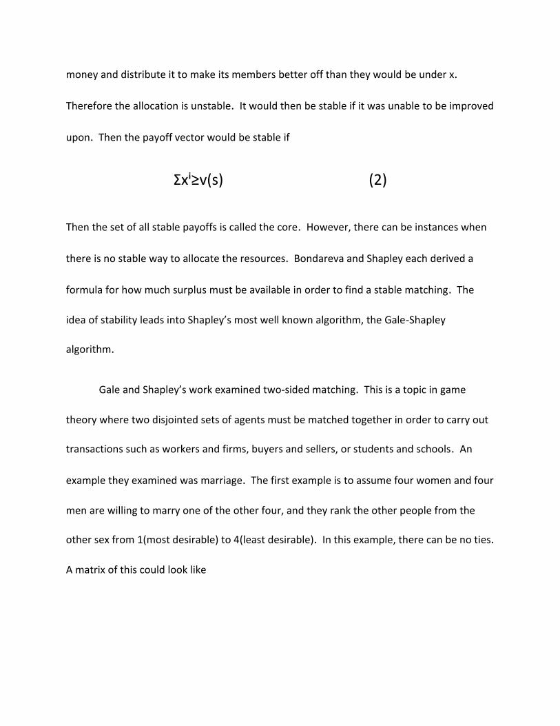
money and distribute it to make its members better off than they would be under x.

Therefore the allocation is unstable. It would then be stable if it was unable to be improved

upon. Then the payoff vector would be stable if

Σxⁱ≥v(s) (2)

Then the set of all stable payoffs is called the core. However, there can be instances when

there is no stable way to allocate the resources. Bondareva and Shapley each derived a

formula for how much surplus must be available in order to find a stable matching. The

idea of stability leads into Shapley’s most well known algorithm, the Gale-Shapley

algorithm.

Gale and Shapley’s work examined two-sided matching. This is a topic in game

theory where two disjointed sets of agents must be matched together in order to carry out

transactions such as workers and firms, buyers and sellers, or students and schools. An

example they examined was marriage. The first example is to assume four women and four

men are willing to marry one of the other four, and they rank the other people from the

other sex from 1(most desirable) to 4(least desirable). In this example, there can be no ties.

A matrix of this could look like

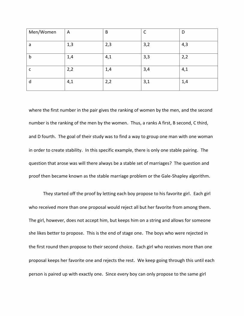
Men/Women A B C D

a 1,3 2,3 3,2 4,3

b 1,4 4,1 3,3 2,2

c 2,2 1,4 3,4 4,1

d 4,1 2,2 3,1 1,4

where the first number in the pair gives the ranking of women by the men, and the second

number is the ranking of the men by the women. Thus, a ranks A first, B second, C third,

and D fourth. The goal of their study was to find a way to group one man with one woman

in order to create stability. In this specific example, there is only one stable pairing. The

question that arose was will there always be a stable set of marriages? The question and

proof then became known as the stable marriage problem or the Gale-Shapley algorithm.

They started off the proof by letting each boy propose to his favorite girl. Each girl

who received more than one proposal would reject all but her favorite from among them.

The girl, however, does not accept him, but keeps him on a string and allows for someone

she likes better to propose. This is the end of stage one. The boys who were rejected in

the first round then propose to their second choice. Each girl who receives more than one

proposal keeps her favorite one and rejects the rest. We keep going through this until each

person is paired up with exactly one. Since every boy can only propose to the same girl

once, every girl is sure to get a proposal in due time. Once this is done, every girl is

required to accept the boy on her string. We then know that this is a stable matching,

because if boy a likes another girl more than his current wife, he has already proposed to

her and has been turned down. Therefore, no one can better their situation by marrying

someone else. This algorithm will also produce a stable arrangement in at most n²-2n+2

where n is the number of people in the two-side matching.

An example of this kind of “deferred-acceptance” procedure could be used in college

admissions. For simplification, a student that would not be accepted under any

circumstances would be automatically denied and would not be considered in this

algorithm. To begin, all students apply to the college of their first choice. The college then

fills up its quota, q, and puts these students on a waiting list. The school then rejects the

rest of the applicants. The students who had their applications denied then apply to their

second choice. This process repeats until every student is matched up with a college, thus

creating stability. The proof that this is stable is analogous to the proof given for the

marriage problem. This matching would be most favorable to the applicants since they get

to make their top choices. The symmetric applicant-proposing version of the algorithm

leads towards an applicant-optimal stable matching. This illustrates the applicants’

interests as opposed to the employer. Because of this, applicants agree this is the best way

to do things, while employers think this is the worst. The opposite of this would then be

employer-optimal stable matching, where the algorithm is sorted to the needs of the

employer and not the student. However, in this case, the applicant-optimal matching

would be best since schools are supposed to be resources for their students.

In the 1980’s Alvin Roth built upon the work that Gale and Shapley did in the 1960’s.

The key contribution that Roth added dealt with the evolution of the market for new

doctors in the U.S. and that a stable algorithm improves the function of the market.

Students who graduate from medical school are often hired as residents at hospitals. Due

to the high competition for these residents, hospitals were makings offers to them

increasingly early, even sometimes years before a student would graduate. These matches

were made before students could produce evidence on how qualified they would be, or

what kind of medicine they planned to practice. The market also suffered from congestion;

when a student rejected an offer, it was often too late for him to apply for another one.

Roth found that this kind of problem was plaguing many markets including the market for

psychology internships, dental residencies, and the markets for Japanese university

graduates. To deal with the problem in the United States, a clearinghouse was introduced

that matched doctors with hospitals using an algorithm which was found to be essentially

equivalent to Gale and Shapley’s. This program is still in place today and uses a form of the

algorithm produced by Gale and Shapley in 1962.

Alvin Roth also looked at school admissions in New York City. Prior to 2003,

applicants to New York City public high schools ranked the five schools they preferred most

and these preference lists were then sent to the schools. The schools then decided which

students to admit and reject. This went on for two more rounds with the remaining

students entering into an administrative process. This process was very congested with

about 30,000 students ending up in the administrative process every year. Another

problem with this system was that students were most likely to be admitted if they ranked

the school as number one. Therefore, if a student did not have a realistic shot at being

accepted into their top choice, it would not be in their best interest to put it as number one.

In 2003, Roth helped refine this process. In this new process, it is optimal for the students

to report their preferences truthfully, and because of this congestion was eliminated.

During its first year in practice, only about 3,000 students had to be matched with schools

for which they had not expressed a preference, a 90% reduction from previous years. This

helped create a stable outcome and helped reach a Nash Equilibrium. Other schools in the

United States also adopted similar algorithms, most recently in the Denver public school

system.

Lloyd Shapley and Alvin Roth’s work also contributed much more to the field of

game theory, helping them win the Nobel Prize. Shapley introduced the main single-valued

solution concept for coalitional games with transferable utility, now called the Shapley

value. This value played a major role in the development of cooperative game theory,

which has a large variety of applications, including government taxations and

redistributions of utilities. Outside of cooperative game theory, Shapley’s research includes

mathematics, atomic games, non-cooperative games, and convex games, just to name a

few. Alvin Roth continued to take many of the theoretical concepts of cooperative game

theory and apply them to real life situations and models. In 1991 he described how

laboratory experiments and field observations can interact with game theory, establishing

economics as more of an empirical science. Roth and his co-authors tested the prediction

of cooperative bargaining theory. Laboratory experiments led him to reveal that subjects

change their behavior over time. This led him to create a reinforcement learning model

that can predict behavior ex ante.

On the surface, the Gale-Shapley algorithm actually involves very little mathematics.

One does not need to know calculus, geometry, or even algebra to understand the flow of

the arguments and examples of the algorithm. However, the mathematics comes from the

flow of the argument and being able to think through the process that the algorithm

creates. Mathematics needs not be concerned with figures, whether numerical or

geometrical. Mathematics is a way of thought and the flow of an argument. The Gale-

Shapley algorithm uses mathematics and in this way, they were able to use their

mathematical backgrounds to expand into the world of economics and, with the help of

Alvin Roth, work to solve real world problems. Because of this, Lloyd Shapley and Alvin

Roth were more than qualified to win the 2012 Nobel Price for economics.

Works Cited

Shapley, L. S., and D. Gale. "Admissions and the Stability of Marriage." The American

Mathematical Monthly 69.1 (1962): 9-15. Print.

Shapley, L. S. A VALUE FOR N-PERSON GAMES. Ft. Belvoir: Defense Technical Information

Center, 1952. Print.

"Stable Allocations and the Practice of Market Design." (n.d.): n. pag. Rpt. in Economic Sciences

Prize Committee of the Royal Swedish Academy of Sciences. Stockholm: Royal Swedish Academy

of Science, 2012.

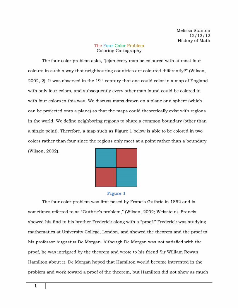
1

Melissa Stanton 12/13/12

History of Math The Four Color ProblemColoring Cartography

The four color problem asks, “[c]an every map be coloured with at most four

colours in such a way that neighbouring countries are coloured differently?” (Wilson,

2002, 2). It was observed in the 19th century that one could color in a map of England

with only four colors, and subsequently every other map found could be colored in

with four colors in this way. We discuss maps drawn on a plane or a sphere (which

can be projected onto a plane) so that the maps could theoretically exist with regions

in the world. We define neighboring regions to share a common boundary (other than

a single point). Therefore, a map such as Figure 1 below is able to be colored in two

colors rather than four since the regions only meet at a point rather than a boundary

(Wilson, 2002).

The four color problem was first posed by Francis Guthrie in 1852 and is

sometimes referred to as “Guthrie’s problem,” (Wilson, 2002; Weisstein). Francis

showed his find to his brother Frederick along with a “proof.” Frederick was studying

mathematics at University College, London, and showed the theorem and the proof to

his professor Augustus De Morgan. Although De Morgan was not satisfied with the

proof, he was intrigued by the theorem and wrote to his friend Sir William Rowan

Hamilton about it. De Morgan hoped that Hamilton would become interested in the

problem and work toward a proof of the theorem, but Hamilton did not show as much

Figure 1

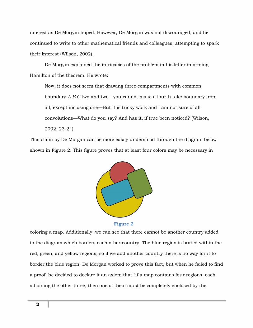
2

interest as De Morgan hoped. However, De Morgan was not discouraged, and he

continued to write to other mathematical friends and colleagues, attempting to spark

their interest (Wilson, 2002).

De Morgan explained the intricacies of the problem in his letter informing

Hamilton of the theorem. He wrote:

Now, it does not seem that drawing three compartments with common

boundary A B C two and two—you cannot make a fourth take boundary from

all, except inclosing one—But it is tricky work and I am not sure of all

convolutions—What do you say? And has it, if true been noticed? (Wilson,

2002, 23-24).

This claim by De Morgan can be more easily understood through the diagram below

shown in Figure 2. This figure proves that at least four colors may be necessary in

coloring a map. Additionally, we can see that there cannot be another country added

to the diagram which borders each other country. The blue region is buried within the

red, green, and yellow regions, so if we add another country there is no way for it to

border the blue region. De Morgan worked to prove this fact, but when he failed to find

a proof, he decided to declare it an axiom that “if a map contains four regions, each

adjoining the other three, then one of them must be completely enclosed by the

Figure 2

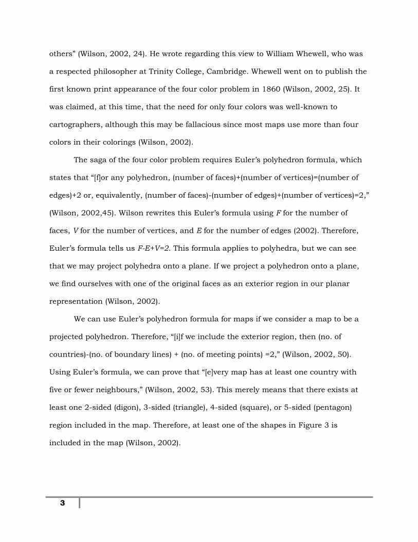
3

others” (Wilson, 2002, 24). He wrote regarding this view to William Whewell, who was

a respected philosopher at Trinity College, Cambridge. Whewell went on to publish the

first known print appearance of the four color problem in 1860 (Wilson, 2002, 25). It

was claimed, at this time, that the need for only four colors was well-known to

cartographers, although this may be fallacious since most maps use more than four

colors in their colorings (Wilson, 2002).

The saga of the four color problem requires Euler’s polyhedron formula, which

states that “[f]or any polyhedron, (number of faces)+(number of vertices)=(number of

edges)+2 or, equivalently, (number of faces)-(number of edges)+(number of vertices)=2,”

(Wilson, 2002,45). Wilson rewrites this Euler’s formula using F for the number of

faces, V for the number of vertices, and E for the number of edges (2002). Therefore,

Euler’s formula tells us F-E+V=2. This formula applies to polyhedra, but we can see

that we may project polyhedra onto a plane. If we project a polyhedron onto a plane,

we find ourselves with one of the original faces as an exterior region in our planar

representation (Wilson, 2002).

We can use Euler’s polyhedron formula for maps if we consider a map to be a

projected polyhedron. Therefore, “[i]f we include the exterior region, then (no. of

countries)-(no. of boundary lines) + (no. of meeting points) =2,” (Wilson, 2002, 50).

Using Euler’s formula, we can prove that “[e]very map has at least one country with

five or fewer neighbours,” (Wilson, 2002, 53). This merely means that there exists at

least one 2-sided (digon), 3-sided (triangle), 4-sided (square), or 5-sided (pentagon)

region included in the map. Therefore, at least one of the shapes in Figure 3 is

included in the map (Wilson, 2002).

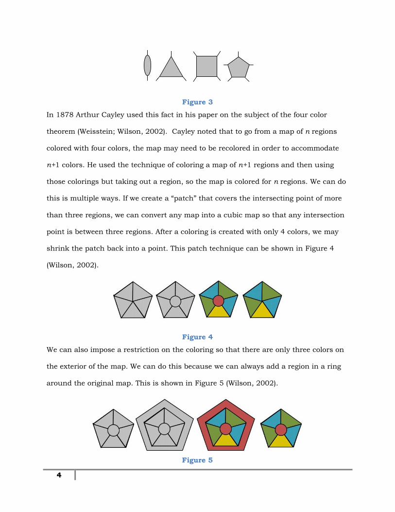
4

In 1878 Arthur Cayley used this fact in his paper on the subject of the four color

theorem (Weisstein; Wilson, 2002). Cayley noted that to go from a map of n regions

colored with four colors, the map may need to be recolored in order to accommodate

n+1 colors. He used the technique of coloring a map of n+1 regions and then using

those colorings but taking out a region, so the map is colored for n regions. We can do

this is multiple ways. If we create a “patch” that covers the intersecting point of more

than three regions, we can convert any map into a cubic map so that any intersection

point is between three regions. After a coloring is created with only 4 colors, we may

shrink the patch back into a point. This patch technique can be shown in Figure 4

(Wilson, 2002).

We can also impose a restriction on the coloring so that there are only three colors on

the exterior of the map. We can do this because we can always add a region in a ring

around the original map. This is shown in Figure 5 (Wilson, 2002).

Figure 3

Figure 4

Figure 5

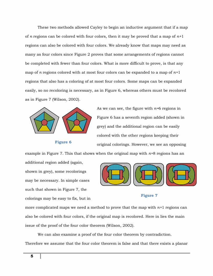
5

These two methods allowed Cayley to begin an inductive argument that if a map

of n regions can be colored with four colors, then it may be proved that a map of n+1

regions can also be colored with four colors. We already know that maps may need as

many as four colors since Figure 2 proves that some arrangements of regions cannot

be completed with fewer than four colors. What is more difficult to prove, is that any

map of n regions colored with at most four colors can be expanded to a map of n+1

regions that also has a coloring of at most four colors. Some maps can be expanded

easily, so no recoloring is necessary, as in Figure 6, whereas others must be recolored

as in Figure 7 (Wilson, 2002).

As we can see, the figure with n=6 regions in

Figure 6 has a seventh region added (shown in

grey) and the additional region can be easily

colored with the other regions keeping their

original colorings. However, we see an opposing

example in Figure 7. This that shows when the original map with n=8 regions has an

additional region added (again,

shown in grey), some recolorings

may be necessary. In simple cases

such that shown in Figure 7, the

colorings may be easy to fix, but in

more complicated maps we need a method to prove that the map with n+1 regions can

also be colored with four colors, if the original map is recolored. Here in lies the main

issue of the proof of the four color theorem (Wilson, 2002).

We can also examine a proof of the four color theorem by contradiction.

Therefore we assume that the four color theorem is false and that there exists a planar

Figure 6

Figure 7

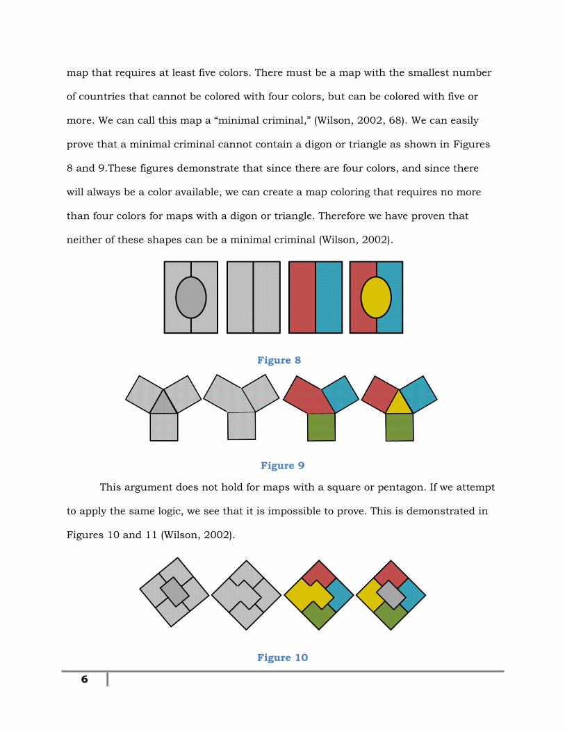
6

map that requires at least five colors. There must be a map with the smallest number

of countries that cannot be colored with four colors, but can be colored with five or

more. We can call this map a “minimal criminal,” (Wilson, 2002, 68). We can easily

prove that a minimal criminal cannot contain a digon or triangle as shown in Figures

8 and 9.These figures demonstrate that since there are four colors, and since there

will always be a color available, we can create a map coloring that requires no more

than four colors for maps with a digon or triangle. Therefore we have proven that

neither of these shapes can be a minimal criminal (Wilson, 2002).

This argument does not hold for maps with a square or pentagon. If we attempt

to apply the same logic, we see that it is impossible to prove. This is demonstrated in

Figures 10 and 11 (Wilson, 2002).

Figure 8

Figure 9

Figure 10

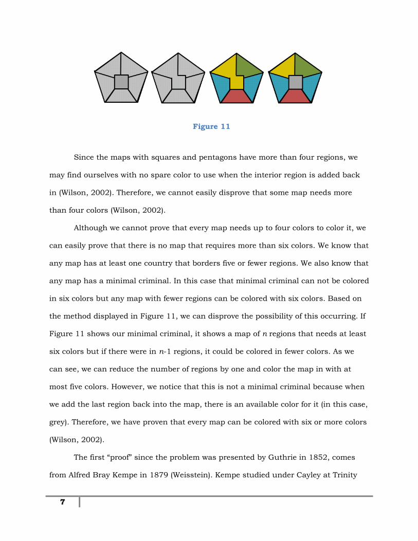
7

Since the maps with squares and pentagons have more than four regions, we

may find ourselves with no spare color to use when the interior region is added back

in (Wilson, 2002). Therefore, we cannot easily disprove that some map needs more

than four colors (Wilson, 2002).

Although we cannot prove that every map needs up to four colors to color it, we

can easily prove that there is no map that requires more than six colors. We know that

any map has at least one country that borders five or fewer regions. We also know that

any map has a minimal criminal. In this case that minimal criminal can not be colored

in six colors but any map with fewer regions can be colored with six colors. Based on

the method displayed in Figure 11, we can disprove the possibility of this occurring. If

Figure 11 shows our minimal criminal, it shows a map of n regions that needs at least

six colors but if there were in n-1 regions, it could be colored in fewer colors. As we

can see, we can reduce the number of regions by one and color the map in with at

most five colors. However, we notice that this is not a minimal criminal because when

we add the last region back into the map, there is an available color for it (in this case,

grey). Therefore, we have proven that every map can be colored with six or more colors

(Wilson, 2002).

The first “proof” since the problem was presented by Guthrie in 1852, comes

from Alfred Bray Kempe in 1879 (Weisstein). Kempe studied under Cayley at Trinity

Figure 11

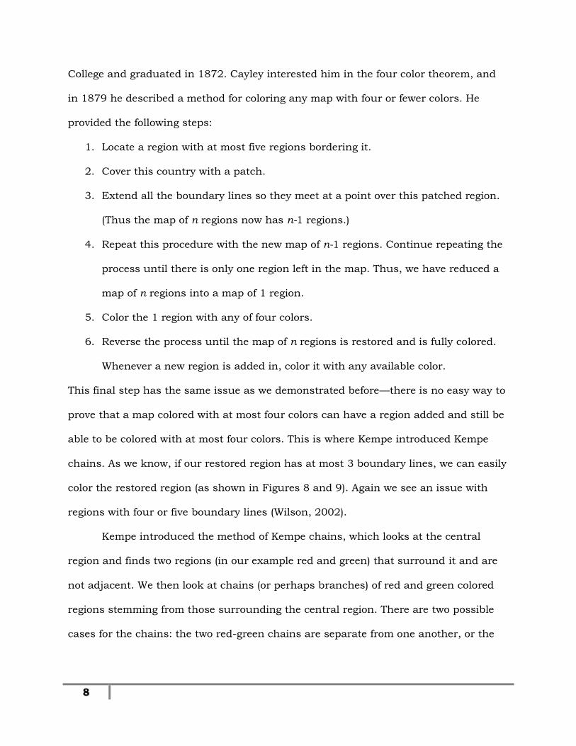
8

College and graduated in 1872. Cayley interested him in the four color theorem, and

in 1879 he described a method for coloring any map with four or fewer colors. He

provided the following steps:

1. Locate a region with at most five regions bordering it.

2. Cover this country with a patch.

3. Extend all the boundary lines so they meet at a point over this patched region.

(Thus the map of n regions now has n-1 regions.)

4. Repeat this procedure with the new map of n-1 regions. Continue repeating the

process until there is only one region left in the map. Thus, we have reduced a

map of n regions into a map of 1 region.

5. Color the 1 region with any of four colors.

6. Reverse the process until the map of n regions is restored and is fully colored.

Whenever a new region is added in, color it with any available color.

This final step has the same issue as we demonstrated before—there is no easy way to

prove that a map colored with at most four colors can have a region added and still be

able to be colored with at most four colors. This is where Kempe introduced Kempe

chains. As we know, if our restored region has at most 3 boundary lines, we can easily

color the restored region (as shown in Figures 8 and 9). Again we see an issue with

regions with four or five boundary lines (Wilson, 2002).

Kempe introduced the method of Kempe chains, which looks at the central

region and finds two regions (in our example red and green) that surround it and are

not adjacent. We then look at chains (or perhaps branches) of red and green colored

regions stemming from those surrounding the central region. There are two possible

cases for the chains: the two red-green chains are separate from one another, or the

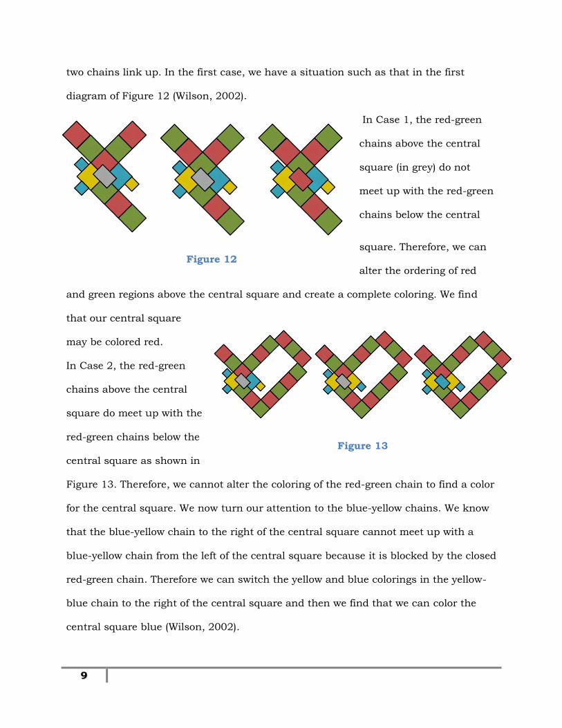
9

two chains link up. In the first case, we have a situation such as that in the first

diagram of Figure 12 (Wilson, 2002).

In Case 1, the red-green

chains above the central

square (in grey) do not

meet up with the red-green

chains below the central

square. Therefore, we can

alter the ordering of red

and green regions above the central square and create a complete coloring. We find

that our central square

may be colored red.

In Case 2, the red-green

chains above the central

square do meet up with the

red-green chains below the

central square as shown in

Figure 13. Therefore, we cannot alter the coloring of the red-green chain to find a color

for the central square. We now turn our attention to the blue-yellow chains. We know

that the blue-yellow chain to the right of the central square cannot meet up with a

blue-yellow chain from the left of the central square because it is blocked by the closed

red-green chain. Therefore we can switch the yellow and blue colorings in the yellow-

blue chain to the right of the central square and then we find that we can color the

central square blue (Wilson, 2002).

Figure 12

Figure 13

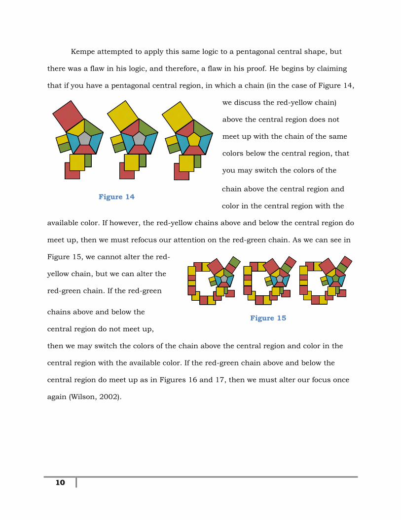
10

Kempe attempted to apply this same logic to a pentagonal central shape, but

there was a flaw in his logic, and therefore, a flaw in his proof. He begins by claiming

that if you have a pentagonal central region, in which a chain (in the case of Figure 14,

we discuss the red-yellow chain)

above the central region does not

meet up with the chain of the same

colors below the central region, that

you may switch the colors of the

chain above the central region and

color in the central region with the

available color. If however, the red-yellow chains above and below the central region do

meet up, then we must refocus our attention on the red-green chain. As we can see in

Figure 15, we cannot alter the red-

yellow chain, but we can alter the

red-green chain. If the red-green

chains above and below the

central region do not meet up,

then we may switch the colors of the chain above the central region and color in the

central region with the available color. If the red-green chain above and below the

central region do meet up as in Figures 16 and 17, then we must alter our focus once

again (Wilson, 2002).

Figure 14

Figure 15

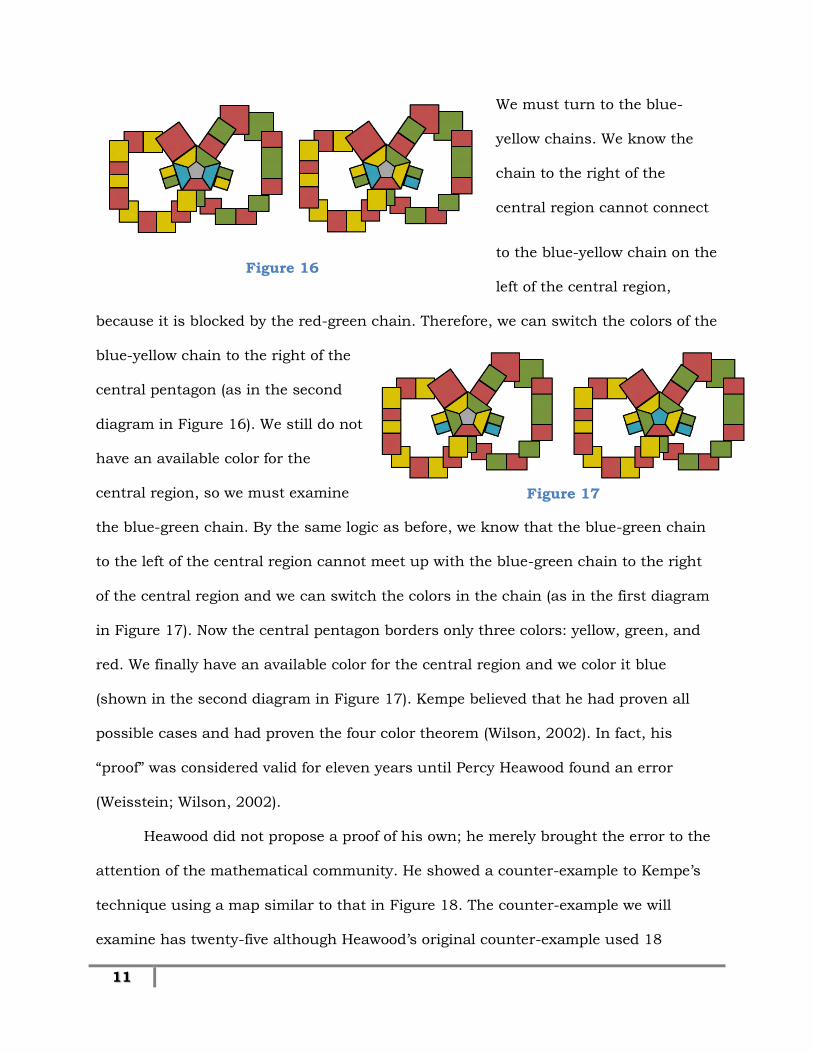
11

We must turn to the blue-

yellow chains. We know the

chain to the right of the

central region cannot connect

to the blue-yellow chain on the

left of the central region,

because it is blocked by the red-green chain. Therefore, we can switch the colors of the

blue-yellow chain to the right of the

central pentagon (as in the second

diagram in Figure 16). We still do not

have an available color for the

central region, so we must examine

the blue-green chain. By the same logic as before, we know that the blue-green chain

to the left of the central region cannot meet up with the blue-green chain to the right

of the central region and we can switch the colors in the chain (as in the first diagram

in Figure 17). Now the central pentagon borders only three colors: yellow, green, and

red. We finally have an available color for the central region and we color it blue

(shown in the second diagram in Figure 17). Kempe believed that he had proven all

possible cases and had proven the four color theorem (Wilson, 2002). In fact, his

“proof” was considered valid for eleven years until Percy Heawood found an error

(Weisstein; Wilson, 2002).

Heawood did not propose a proof of his own; he merely brought the error to the

attention of the mathematical community. He showed a counter-example to Kempe’s

technique using a map similar to that in Figure 18. The counter-example we will

examine has twenty-five although Heawood’s original counter-example used 18

Figure 16

Figure 17

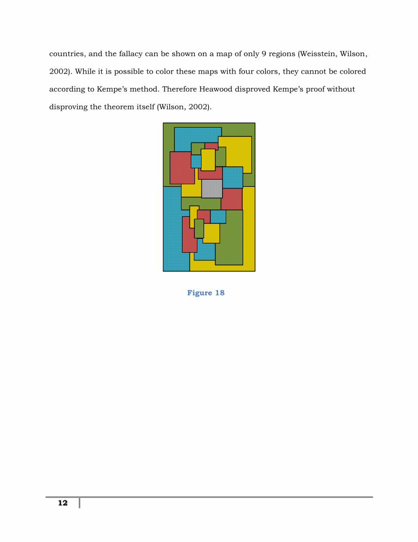
12

countries, and the fallacy can be shown on a map of only 9 regions (Weisstein, Wilson,

2002). While it is possible to color these maps with four colors, they cannot be colored

according to Kempe’s method. Therefore Heawood disproved Kempe’s proof without

disproving the theorem itself (Wilson, 2002).

Figure 18

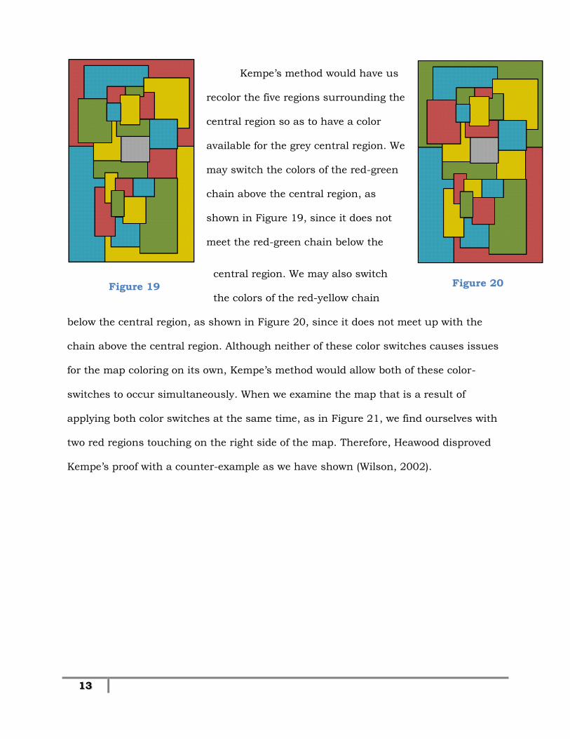
13

Kempe’s method would have us

recolor the five regions surrounding the

central region so as to have a color

available for the grey central region. We

may switch the colors of the red-green

chain above the central region, as

shown in Figure 19, since it does not

meet the red-green chain below the

central region. We may also switch

the colors of the red-yellow chain

below the central region, as shown in Figure 20, since it does not meet up with the

chain above the central region. Although neither of these color switches causes issues

for the map coloring on its own, Kempe’s method would allow both of these color-

switches to occur simultaneously. When we examine the map that is a result of

applying both color switches at the same time, as in Figure 21, we find ourselves with

two red regions touching on the right side of the map. Therefore, Heawood disproved

Kempe’s proof with a counter-example as we have shown (Wilson, 2002).

Figure 19 Figure 20

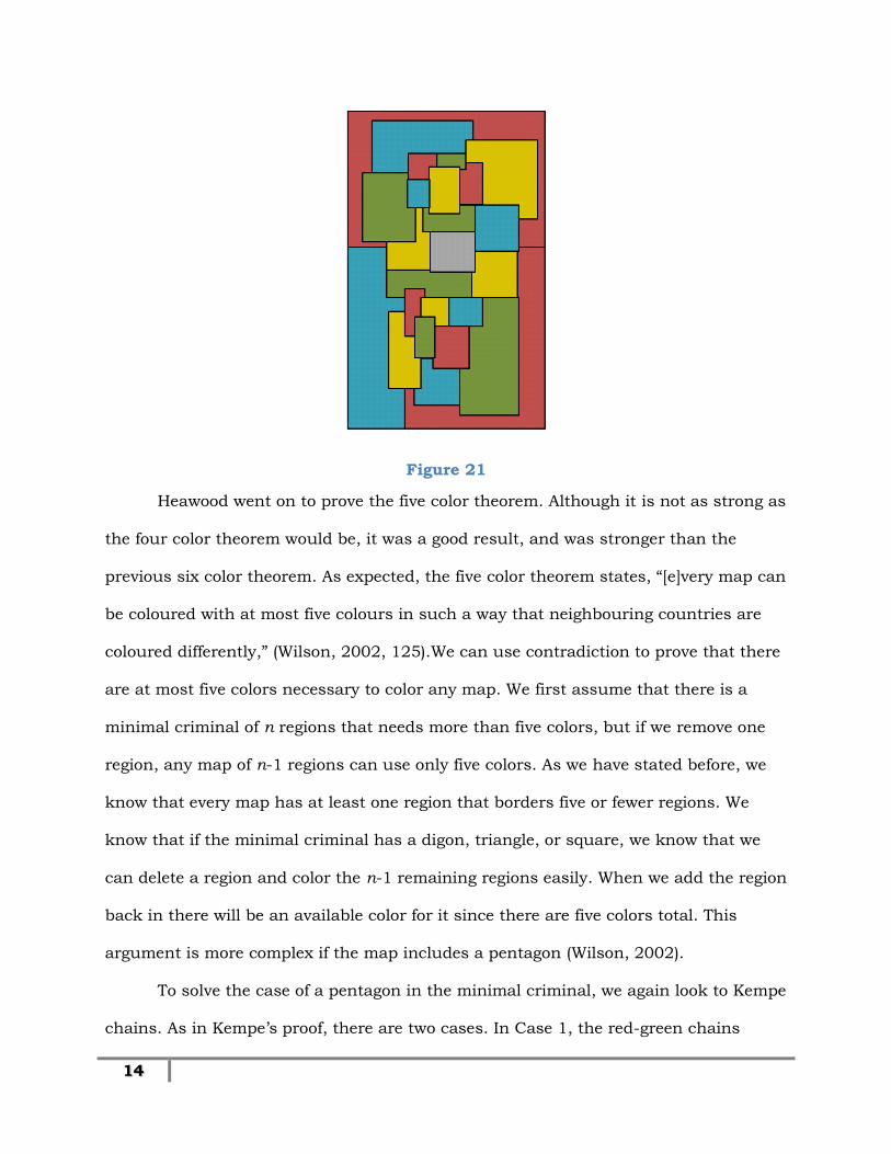
14

Heawood went on to prove the five color theorem. Although it is not as strong as

the four color theorem would be, it was a good result, and was stronger than the

previous six color theorem. As expected, the five color theorem states, “[e]very map can

be coloured with at most five colours in such a way that neighbouring countries are

coloured differently,” (Wilson, 2002, 125).We can use contradiction to prove that there

are at most five colors necessary to color any map. We first assume that there is a

minimal criminal of n regions that needs more than five colors, but if we remove one

region, any map of n-1 regions can use only five colors. As we have stated before, we

know that every map has at least one region that borders five or fewer regions. We

know that if the minimal criminal has a digon, triangle, or square, we know that we

can delete a region and color the n-1 remaining regions easily. When we add the region

back in there will be an available color for it since there are five colors total. This

argument is more complex if the map includes a pentagon (Wilson, 2002).

To solve the case of a pentagon in the minimal criminal, we again look to Kempe

chains. As in Kempe’s proof, there are two cases. In Case 1, the red-green chains

Figure 21

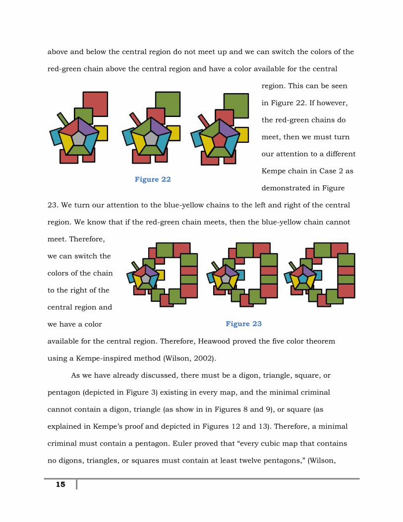
15

above and below the central region do not meet up and we can switch the colors of the

red-green chain above the central region and have a color available for the central

region. This can be seen

in Figure 22. If however,

the red-green chains do

meet, then we must turn

our attention to a different

Kempe chain in Case 2 as

demonstrated in Figure

23. We turn our attention to the blue-yellow chains to the left and right of the central

region. We know that if the red-green chain meets, then the blue-yellow chain cannot

meet. Therefore,

we can switch the

colors of the chain

to the right of the

central region and

we have a color

available for the central region. Therefore, Heawood proved the five color theorem

using a Kempe-inspired method (Wilson, 2002).

As we have already discussed, there must be a digon, triangle, square, or

pentagon (depicted in Figure 3) existing in every map, and the minimal criminal

cannot contain a digon, triangle (as show in in Figures 8 and 9), or square (as

explained in Kempe’s proof and depicted in Figures 12 and 13). Therefore, a minimal

criminal must contain a pentagon. Euler proved that “every cubic map that contains

no digons, triangles, or squares must contain at least twelve pentagons,” (Wilson,

Figure 22

Figure 23

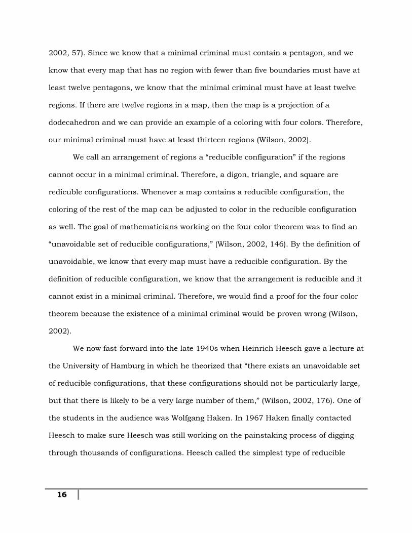
16

2002, 57). Since we know that a minimal criminal must contain a pentagon, and we

know that every map that has no region with fewer than five boundaries must have at

least twelve pentagons, we know that the minimal criminal must have at least twelve

regions. If there are twelve regions in a map, then the map is a projection of a

dodecahedron and we can provide an example of a coloring with four colors. Therefore,

our minimal criminal must have at least thirteen regions (Wilson, 2002).

We call an arrangement of regions a “reducible configuration” if the regions

cannot occur in a minimal criminal. Therefore, a digon, triangle, and square are

redicuble configurations. Whenever a map contains a reducible configuration, the

coloring of the rest of the map can be adjusted to color in the reducible configuration

as well. The goal of mathematicians working on the four color theorem was to find an

“unavoidable set of reducible configurations,” (Wilson, 2002, 146). By the definition of

unavoidable, we know that every map must have a reducible configuration. By the

definition of reducible configuration, we know that the arrangement is reducible and it

cannot exist in a minimal criminal. Therefore, we would find a proof for the four color

theorem because the existence of a minimal criminal would be proven wrong (Wilson,

2002).

We now fast-forward into the late 1940s when Heinrich Heesch gave a lecture at

the University of Hamburg in which he theorized that “there exists an unavoidable set

of reducible configurations, that these configurations should not be particularly large,

but that there is likely to be a very large number of them,” (Wilson, 2002, 176). One of

the students in the audience was Wolfgang Haken. In 1967 Haken finally contacted

Heesch to make sure Heesch was still working on the painstaking process of digging

through thousands of configurations. Heesch called the simplest type of reducible

17

configurations “D-reducible,” and he called the type of configurations that could be

reduced but required a proof “C-reducible” (Wilson, 2002).

Haken began to use a computer to check cases. Issues quickly arose when the

computer time grew too large to handle cases. The time to check a configuration with a

ring size eleven was doable, but once the ring size increased by even one region, the

computer time was increased by roughly a factor of four. Haken showed his work to

Heesch and they attempted to create a more efficient method which could decrease the

computer time necessary (Wilson, 2002).

Most mathematicians working on a proof set their sights on a collecting

reducible configurations and then creating a set of them. Haken decided to create a set

of “configurations that were likely to be reducible—in particular, they should contain

none of the reduction obstacles—in order to avoid wasting time checking

configurations” that were unnecessary (Wilson, 2002, 193-194). Haken began working

with Kenneth Appel who handled most of the computing aspect of the problem. The

two began in 1972 and finally found success in 1976. The two formally released their

work on July 22, 1976 to colleagues and published their solution to the Illinois Journal

of Mathematics in December 1977 (Wilson, 2002).

The proof was long-awaited, and yet found a lukewarm reception by the

mathematical community. There were a variety of responses, but the overwhelming

reaction, especially from those older than around forty, was disaproval regarding the

proof method. The four color proof sparked a debate regarding, philosophically, what

exactly constitutes a proof. The mathematicians who were slightly older when the

proof was released were concerned by the extent the computer was used and whether

anyone could be confident that there were no errors. The slightly younger

mathematicians tended to have fewer issues accepting a computer-assisted proof.

18

They instead argued that a long, complicated proof that was checked entirely by hand

had a great possibility for human error and could just as easily contain mistakes.

Even Kempe’s proof of the four color theorem was accepted for over a decade before

his error was found by Heawood (Wilson, 2002).

In this way, the four color theorem was proved 124 years after it was first

introduced to the mathematical community. Although it has had a long and sordid

history including a false proof by Kempe and a long-awaited but antagonistically

accepted computer-accepted proof, the four color theorem has finally been shown to

be true (Wilson, 2002).

Works Cited:

Weisstein, E. W. (n.d.). Four-Color Theorem. Wolfram MathWorld: The Web's Most

Extensive Mathematics Resource. Retrieved from

http://mathworld.wolfram.com/Four-ColorTheorem.html

Wilson, R. J. (2002). Four colors suffice: How the map problem was solved. Princeton,

NJ: Princeton University Press.