Embed Size (px)
Citation preview
Historical Trends in Social Mobility: Data, Methods, and Farming
Yu Xie
Alexandra Killewald
University of Michigan
Population Studies Center Research Report 10-716
August 2010
_____________
Please direct all correspondence to Yu Xie (e-mail: [email protected]) at Population Studies Center, Institute for Social Research, 426 Thompson Street, University of Michigan, Ann Arbor, MI 48106. We thank Joseph Ferrie for sharing data with us, Zheng Mu and Robert Willis for comments and suggestions on the paper, Miriam King for advice on historical census data, and Cindy Glovinsky for editorial assistance.
Historical Trends in Social Mobility: Data, Methods, and Farming 2
ABSTRACT Using historical census data and survey data, Ferrie and Long (forthcoming) found a significant decline in social mobility in the United States from 1880 to 1973. We present three critiques of the Ferrie-Long study. First, the data quality of the Ferrie-Long study is far more limiting than the authors acknowledge, and we are able to detect some bias in their data in favor of their conclusion. Second, the Ferrie-Long study capitalizes on a particular method that is highly sensitive to an operationalization of the concept “social mobility.” Third, almost all the findings of the Ferrie-Long study are driven by farmers.

Historical Trends in Social Mobility: Data, Methods, and Farming 3
INTRODUCTION
Social scientists in general, and sociologists in particular, have long been interested in intergenerational occupational mobility. Indeed, the interest is so common in sociology that intergenerational occupational mobility is referred to there simply as “social mobility.” Most notable among innumerable contributions to the large literature on social mobility are landmark studies of Blau and Duncan (1967) and Featherman and Hauser (1978) for the U.S. and of Erikson and Goldthorpe (1992) for Europe. In these studies, social mobility is taken to measure a society’s openness. A widely accepted view rooted in neoclassical liberalism is that more social mobility, i.e., more openness, is good for a society, as it encourages placement of individuals in social positions according to competence rather than social origin (Hout 1988). Adding to this large literature on social mobility is now a well-researched study by economists Ferrie and Long (forthcoming). Using historical census data and survey data, the Ferrie-Long study compares the U.S. and Britain around 1880 and around 1973. A key finding of the study is that the United States was much more socially mobile than Britain in the period around 1880, but the two countries had similar levels of social mobility around 1973. The authors supplemented the core comparison of the four (2x2) datasets with the analysis of four additional datasets for the U.S., demonstrating a sharp decline in social mobility in the U.S. over its history of rapid industrialization and economic expansion from the post-Civil War era to the post-World War II era. Thus, the Ferrie-Long study supports the popular conception of America as an exceptional land of opportunity for all, but only prior to 1900. The findings of the Ferrie-Long study are bound to shock the community of scholars who have been studying social mobility. Beginning with Lipset and Bendix (1964) if not earlier, the sociological literature on comparative social mobility now dates back more than fifty years (Ganzeboom, Treiman, Ultee 1991). The dominant view in the literature is that relative social mobility, or social fluidity (to be defined below), is either constant, or trendless and patternless in all industrialized nations (Featherman, Jones, and Hauser 1975; Erikson and Goldthorpe 1992; Guest, Landale and McCann 1989; Grusky and Hauser 1984; Hauser et al. 1975). A main challenge to this dominant view, based on empirical studies, is that social mobility in industrialized nations has increased over time, albeit slowly (e.g., Breen and Jonsson 2007; Featherman and Hauser 1978; Grusky1986; Hout 1988; Vallet 2001). To our knowledge, Ferrie and Long are the first scholars to argue for the significant decline of social mobility in a major modern society. Given this controversial conclusion, whether or not the evidence actually supports their argument is of great interest to the larger scholarly community.
Historical Trends in Social Mobility: Data, Methods, and Farming 4
Why are the key findings of the Ferrie-Long study so different from those in a long and
well-established standard literature on comparative social mobility? While most scholars who
study social mobility are sociologists with a widely-accepted but confined paradigm, Ferrie and
Long are economists who use methods and data that have not been widely used in sociology.
Thus, the Ferrie-Long study is valuable in providing both new data on historical social mobility
in the U.S. and Britain and a new challenge to the dominant “trendless” view found in the
sociology literature on comparative mobility. However, before we can accept the findings of the
Ferrie-Long study, we need to fully understand the study and its limitations and explore
alternative interpretations.
In this paper, we present our critique of the Ferrie-Long study. While the Ferrie-Long
study yielded many results, its most surprising finding was that the pre-1900 U.S. was much
more socially mobile than the post-1970 U.S. Our critique thus focuses on the long-term trend
analysis in the study of the U.S. case. Our critique can be summarized by three main points. First,
the data quality of the Ferrie-Long study is far more limiting than the authors acknowledge, and
we are able to detect some bias in their data in favor of their conclusion. Second, the Ferrie-Long
study capitalizes on a particular method that is highly sensitive to an operationalization of the
concept “social mobility.” Third, almost all the findings of the Ferrie-Long study are driven by
farmers, who have not only constituted a unique sector in the labor market but also experienced a
tremendous decline in the U.S. labor force since 1880.
HISTORICAL CENSUS DATA
A major contribution of the Ferrie-Long study is its creative use of historical census data.
For simplicity, we focus our discussion on the U.S. data, as these data give rise to the surprising
finding we discussed earlier. The basic idea is to link individuals (white males) across different
censuses by name, state of birth (and parents’ states of birth), and year of birth. The linkage
procedure capitalizes on the fact that, while only (1 percent) samples of families are available
from the 1850, 1860, and 1900 U.S. censuses (http://usa.ipums.org/), the complete enumerations
of the 1880 U.S. census are available (http://www.nappdata.org/). Appendix 1 of the Ferrie and
Long (forthcoming) paper provides detailed documentation for linkages between the 1850 census
and the 1880 census for white males ages 25 and under in 1850. We assume that the experience
documented for 1850-1880 linkages is also applicable to those for 1860-1880 and 1880-1900
linkages that were also performed by the authors.

Historical Trends in Social Mobility: Data, Methods, and Farming 5
The authors acknowledge certain limitations of the data resulting from this linking
procedure, documenting a 22 percent success rate for “white males age 25 and under in 1850”
(Ferrie and Long forthcoming, p.37).1
Our evaluation of the data quality proceeds in two steps. First, we document a data quality
issue that is ignored in the Ferrie-Long study and its potential consequence for biases. Second,
we provide some concrete evidence that suggests a bias resulting from their linking procedure in
favor of Ferrie and Long’s conclusion.
However, the question still lingers as to whether the
matched data are of sufficient quality, especially given a high failure rate of 78 percent. If the
occurrence of matching failures were truly random, as the authors assume, the low success rate
would have not caused any bias to the results. In the other extreme scenario of strong sample
selection, however, the sample of successfully matched cases would have provided little
identifying information about the general population to which the authors wish to generalize
(Manski 1995). Thus, it is extremely important that we evaluate the quality of the matched data
from historical censuses.
One data issue that is not discussed by Ferrie and Long in their paper is the requirement of
coresidence with fathers on the earlier census. For example, in order to construct the
intergenerational mobility table by matching data from the 1850 and 1880 U.S. censuses, it is
necessary that boys ages 13-19 be reported to co-reside with their fathers on the 1850 census
form, as we also need the father-son linkage on the 1850 census form to know father’s
occupation (in 1850). Not all young white males lived with their fathers. Using data from the
Integrated Public Use Microdata Series (IPUMS) (Ruggles et al. 2009), we examine the
residential status of boys of the ages considered in the Ferrie and Long study. In our reanalysis of
the 1850 data, we find the percentage of coresidence to be 72% for white males ages 0-25 and
68% for white males ages 13-19.2
As expected, the coresidence rate differs by age, farm status,
and student status. We provide full descriptive statistics involving these variables in Table 1.
1 We are unclear as to why the documentation refers to white males ages 25 and under in 1850, as the authors actually used data for white males between ages 13 and 19 in their main mobility analysis reported in the paper. In our reanalysis of the data, we do not find the matching rate to differ much as we change the age range from 0-25 to 13-19. 2 Our reanalysis of the Ferrie-Long data focuses on linkages between the 1850 and 1880 censuses because this is the matched data that were provided to us by Joseph Ferrie. Appendix 1 of the Ferrie and Long paper also discusses the 1850-1880 linkages extensively.

Historical Trends in Social Mobility: Data, Methods, and Farming 6
Table 1: Estimated Statistics for Young White Males in 1850 U.S.
Farm Non-Farm In School Not in School0-25 54.8 32.5 72.7 80.4 63.5 85.9 66.4
13-19 58.1 43.9 68.6 78.1 55.3 81.3 58.6
13 60.7 66.5 80.7 87.0 71.0 83.8 74.514 58.3 62.1 77.5 84.2 68.1 81.5 71.015 60.4 54.8 75.3 82.4 64.4 82.1 67.016 58.9 43.9 70.5 79.4 57.6 81.3 62.017 58.2 34.5 64.6 75.0 50.0 79.3 56.818 55.1 23.8 57.5 70.1 42.0 79.1 50.719 54.8 18.1 51.7 65.6 34.8 75.8 46.3
Source: IPUMS of the 1850 US Census
% On Farm% In
SchoolAge
% Living with Father
Totalby Farm Status by Student Status
The first two columns of Table 1 show that, in 1850, 58% of U.S. white boys ages 13-19 lived on farms, and 44% of them were enrolled as students. Negative age graduations are clear for both variables, although the age pattern for enrollment is much more pronounced. These negative age patterns suggest that young Americans then were already leaving school as well as home at these young ages. Note that the percentage of being enrolled in school was only at 67% for 13 years old boys.3
Hence, we have shown that occupational mobility is structurally unknown for a large portion (about a third) of youth in the Ferrie and Long data due to their data construction method, even in the unlikely event of no linkage failures. Moreover, there are systematic patterns of this data omission by age, farm status, and student status. We do not know how this data limitation may have caused biases to the social mobility tables in the Ferrie-Long study. At the minimum, however, our reanalysis of the original 1850 data has revealed that that the actual matching rate
For these reasons, we are not surprised to observe, in the third column, that only 69% of young men in this age range still lived with their fathers, with the percentage declining gradually from 81% at age 13 to 52% at age 19. The last four columns break down the likelihood of coresidence by farm status and school status, with living on farms and being enrolled in schools both positively associated with coresidence with fathers. Again, there is a negative age pattern within each group.
3 This low enrollment is not surprising, given that a large fraction of adult Americans (more precisely, 10% for whites age 20-50) were still illiterate in 1850 (calculated from http://usa.ipums.org/usa/sda/).
Historical Trends in Social Mobility: Data, Methods, and Farming 7
between the 1850 and 1880 censuses in the Ferrie-Long study is not 22 percent as reported, but much worse, 22 percent of 69 percent, i.e., 15 percent.
Conditional on coresidence, the probability of finding a match between the 1850 and 1880 data may be correlated with intergenerational mobility.4 Of course, ideally, we wish to know whether or not the matching likelihood is associated with intergenerational mobility in 1880, but this missing-at-random assumption cannot be empirically evaluated, as we do not observe a person’s occupation in 1880 unless the case is successfully matched. However, for a subset of sons who were already employed in occupations in 1850, it is possible to construct an intergenerational occupational mobility table based on 1850 data alone. Of course, the mobility experiences of this highly selective subsample should not be representative of their peers who did not report an occupation in 1850.5
To be conservative, we further restrict our analysis in Table 2 to young white males who not only co-resided with father and reported occupation, but also were not enrolled in school. We make this restriction to ensure that occupations reported for these sons in 1850 reflected their real jobs, not part-time jobs held by students. In Panel 1, we present the 1850 mobility table for the matched subsample; in Panel 2, we present the 1850 mobility table for the unmatched subsample. Again, matching is with respect to the 1880 census and thus could not possibly affect the 1850 mobility table in the way it does the 1880 mobility table. In Panel 3, we use the same method for evaluating social mobility in the two tables as in the Ferrie and Long study, although we realize the limitations of the method and will discuss them in the next section. We observe
In addition, many of these young persons would have changed to different occupations in 1880. Thus, a mobility table based on 1850 data for this special group is of limited substantive value, but it can be used to shed light on the issue of potential biases associated with matching. The main idea is to break the 1850 mobility table by matching status (success versus failure). If matching success or failure is truly random, mobility tables for the two subgroups broken down by matching status should not differ. That is, there is no reason, a priori, that mobility patterns within this group should differ on the basis of their “future” matching status, unless matching is selective on mobility, which is then a testable hypothesis. We report our results of this test in Table 2.
4 We conducted an analysis of the likelihood of matching as a function of 1850 characteristics. We found that living in an urban (rather than a rural) place, having fewer siblings, father being literate (rather than illiterate), and being enrolled in school were all positively associated with matching success. Ferrie and Long also conducted a similar analysis and constructed weights to account for differential likelihoods of matching based on observed covariates. 5 In fact, among the matched members of our subsample, the d index (with I as reference) for the 1850-1880 intergenerational mobility is 16.0, somewhat larger than what is reported by Ferrie and Long for this whole cohort, at 11.9 (from the 1850-1880 data) or 12.1 (from the 1860-1880 data).

Historical Trends in Social Mobility: Data, Methods, and Farming 8
that the matched subsample (P, in Panel 1) is more mobile (i.e., closer to I, standing for independence) than the unmatched subsample (Q, in Panel 2). The results are:6
d(P,I) = 29.89 d(Q,I) = 33.56 d(P,Q) = 7.71
Table 2: Intergenerational Mobility for Fathers and Sons in U.S. 1850
Son's Occupation White Collar FarmerSkilled/
Semiskilled Unskilled Row SumPanel 1. Matched Subsample (P)
White Collar 15 7 12 4 38(45.5) (2.3) (11.9) (11.8)
Farmer 3 204 17 2 226(9.1) (66.4) (16.8) (5.9)
Skilled/Semiskilled 11 8 59 7 85(33.3) (2.6) (58.4) (20.6)
Unskilled 4 88 13 21 126(12.1) (28.7) (12.9) (61.8)
Column Sum 33 307 101 34 475
Panel 2. Unmatched Subsample (Q)White Collar 57 13 34 7 111
(55.9) (1.3) (9.1) (5.5)Farmer 14 747 65 6 832
(13.7) (72.3) (17.4) (4.7)Skilled/Semiskilled 19 15 207 28 269
(18.6) (1.5) (55.5) (21.9)Unskilled 12 258 67 87 424
(11.8) (25.0) (18.0) (68.0)Column Sum 102 1033 373 128 1636
Panel 3. Summay Measures of Mobility in Matched and Unmatched Subsamples
d(P,I) G 2 d(Q,I) G 2 d(P,Q) G 2
29.89 278.29 33.56 1067.16 7.71 6.7
Father's Occupation
Source: IPUMS of the 1850 US Censuse, with matching identification provided by Joseph Ferrie. See Ferrie and Long (forthcoming).
Note: The sample is restricted to father-son pairs in which the son was age 13-19 in 1850, both father and son reported an occupation in 1850, and the son was not enrolled in school.
6 We also note that the test for differences in odds-ratios between the two tables is not statistically significant.

Historical Trends in Social Mobility: Data, Methods, and Farming 9
These d indexes are larger than those reported for the 1880 U.S. in the Ferrie-Long study.
As we discussed before, the numbers are not comparable in an absolute sense. Because persons
in mobility tables in Table 2 were somewhat selective and young (13-19 years old), the absolute
magnitude of the d indexes is of no interest. The importance of the results in Table 2 lies in
revealing a bias in the matched data that are analyzed by Ferrie and Long -- a bias indeed in
favor of their key finding of high mobility in 1880, as the matched subsample shows moderately
more mobility than in the unmatched subsample ((d(P,I) = 29.9) versus d(Q,I) = 33.6). The
difference in mobility between the two tables is noticeable (d(P,Q) = 7.7) but fairly small in
magnitude. To conclude, if there had been no matching failures, or matching success or failure
had been truly random, we have good reasons to infer that the mobility table for 1880 would
show less social mobility than reported in the Ferrie-Long study. However, we do not think that
this bias alone would account for the unusual finding in the Ferrie-Long study.
MEASURING SOCIAL MOBILITY
Measurement of social mobility is not a straightforward matter. For the benefit of readers
who may not be familiar with the sociological literature on social mobility, we present a brief
methodological review in this section. Since an intergenerational mobility table is usually a
square matrix, with the same occupational classification for father’s occupation and son’s
occupation, diagonal cells represent immobility, or inheritance. At the first glance, it seems that
we can simply measure social mobility by the proportion of individuals who fall in off-diagonal
cells in a mobility table. Indeed, this simple descriptive measure, called “total mobility rate,”
“absolute mobility rate,” or simply “mobility rate,” is commonly used and reported, as in the
Ferrie-Long study. Of course, methodological problems with the mobility rate have been well
known for a long time (Ganzeboom, Treiman, Ultee 1991). The main problem is that the
mobility rate is affected by the marginal distributions of a mobility table.
Let ijf be the observed frequency in the ith row ( 1,..i I= ) and jth column ( 1,..j I= ) in a
mobility table with I rows and I columns. We follow Ferrie and Long in representing son’s
occupation in rows and father’s occupation in columns, although the convention in the standard
mobility literature is the reverse.
Historical Trends in Social Mobility: Data, Methods, and Farming 10
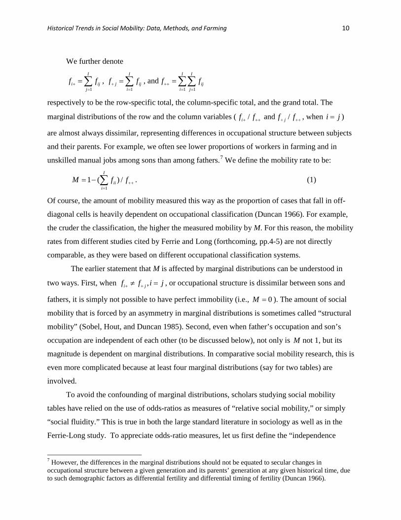
We further denote
1
I
i ijj
f f+=
=∑ , 1
I
j iji
f f+=
=∑ , and1 1
I I
iji j
f f++= =
=∑∑
respectively to be the row-specific total, the column-specific total, and the grand total. The
marginal distributions of the row and the column variables ( /if f+ ++ and /jf f+ ++ , when i j= )
are almost always dissimilar, representing differences in occupational structure between subjects
and their parents. For example, we often see lower proportions of workers in farming and in
unskilled manual jobs among sons than among fathers.7
11 ( ) /
I
iii
M f f++=
= − ∑
We define the mobility rate to be:
. (1)
Of course, the amount of mobility measured this way as the proportion of cases that fall in off-
diagonal cells is heavily dependent on occupational classification (Duncan 1966). For example,
the cruder the classification, the higher the measured mobility by M. For this reason, the mobility
rates from different studies cited by Ferrie and Long (forthcoming, pp.4-5) are not directly
comparable, as they were based on different occupational classification systems.
The earlier statement that M is affected by marginal distributions can be understood in
two ways. First, when ,i jf f i j+ +≠ = , or occupational structure is dissimilar between sons and
fathers, it is simply not possible to have perfect immobility (i.e., 0M = ). The amount of social
mobility that is forced by an asymmetry in marginal distributions is sometimes called “structural
mobility” (Sobel, Hout, and Duncan 1985). Second, even when father’s occupation and son’s
occupation are independent of each other (to be discussed below), not only is M not 1, but its
magnitude is dependent on marginal distributions. In comparative social mobility research, this is
even more complicated because at least four marginal distributions (say for two tables) are
involved.
To avoid the confounding of marginal distributions, scholars studying social mobility
tables have relied on the use of odds-ratios as measures of “relative social mobility,” or simply
“social fluidity.” This is true in both the large standard literature in sociology as well as in the
Ferrie-Long study. To appreciate odds-ratio measures, let us first define the “independence
7 However, the differences in the marginal distributions should not be equated to secular changes in occupational structure between a given generation and its parents’ generation at any given historical time, due to such demographic factors as differential fertility and differential timing of fertility (Duncan 1966).
Historical Trends in Social Mobility: Data, Methods, and Farming 11
model” by the null hypothesis that there is no statistical association between father’s occupation
and son’s occupation. The independence model is usually taken as the natural reference point for
perfect mobility, deviation from which is then taken to indicate social closure, or social
immobility. If the row and the column variables are independent of each other, it is easy to
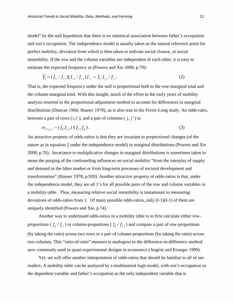
estimate the expected frequency as (Powers and Xie 2008, p.70):
( / )( / ) /ij i j i jf f f f f f f f f+ ++ + ++ ++ + + ++= = . (2)
That is, the expected frequency under the null is proportional both to the row-marginal total and
the column-marginal total. With this insight, much of the effort in the early years of mobility
analysis resorted to the proportional-adjustment method to account for differences in marginal
distributions (Duncan 1966; Hauser 1978), as is also true in the Ferrie-Long study. An odds-ratio,
between a pair of rows ( , 'i i ), and a pair of columns ( , 'j j ) is:
, '; , ' ' ' ' '( ) /( )i i j j ij i j i j ijf f f fω = . (3)
An attractive property of odds-ratios is that they are invariant to proportional changes (of the
nature as in equation 2 under the independence model) in marginal distributions (Powers and Xie
2008, p.76). Invariance to multiplicative changes in marginal distributions is sometimes taken to
mean the purging of the confounding influences on social mobility “from the interplay of supply
and demand in the labor market or from long-term processes of societal development and
transformation” (Hauser 1978, p.920). Another attractive property of odds-ratios is that, under
the independence model, they are all 1’s for all possible pairs of the row and column variables in
a mobility table. Thus, measuring relative social immobility is tantamount to measuring
deviations of odds-ratios from 1. Of many possible odds-ratios, only (I-1)(I-1) of them are
uniquely identified (Powers and Xie, p.74).
Another way to understand odds-ratios in a mobility table is to first calculate either row-
proportions ( /ij if f + ) or column-proportions ( /ij jf f+ ) and compare a pair of row-proportions
(by taking the ratio) across two rows or a pair of column-proportions (by taking the ratio) across
two columns. This “ratio-of-ratio” measure is analogous to the difference-in-difference method
now commonly used in quasi-experimental designs in economics (Angrist and Krueger 1999).
Yet, we will offer another interpretation of odds-ratios that should be familiar to all of our
readers. A mobility table can be analyzed by a multinomial logit model, with son’s occupation as
the dependent variable and father’s occupation as the only independent variable that is
Historical Trends in Social Mobility: Data, Methods, and Farming 12
categorical. In this setup, only (I-1)(I-1) logit coefficients are identified. Odds-ratios are
exponentiated forms of these logit coefficients. Because we in this case only have a single
categorical independent variable, and logit coefficients are symmetric between the dependent
variable and the independent variable, we can obtain the same logit coefficients, hence the same
odds-ratios, by regressing father’s occupation (as the dependent variable) on son’s occupation.
The first logit regression is an analysis of outflows, whereas the second logit regression is an
analysis of inflows. The two approaches are statistically equivalent, as far as the relevant logit
parameters are concerned.
Also focusing on odds-ratios, the Ferrie-Long study relies on Altham’s (1970) index as the
main method of yielding findings. While it has not been widely used in previous research on
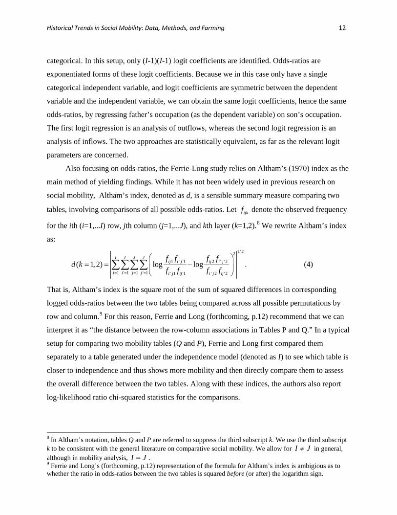
social mobility, Altham’s index, denoted as d, is a sensible summary measure comparing two
tables, involving comparisons of all possible odds-ratios. Let ijkf denote the observed frequency
for the ith (i=1,...I) row, jth column (j=1,...J), and kth layer (k=1,2).8
1/ 22
1 ' '1 2 ' '2
1 ' 1 1 ' 1 ' 1 '1 ' 2 '2
( 1, 2) log logI I J J
ij i j ij i j
i i j j i j ij i j ij
f f f fd k
f f f f= = = =
= = −
∑∑∑∑
We rewrite Altham’s index
as:
. (4)
That is, Altham’s index is the square root of the sum of squared differences in corresponding
logged odds-ratios between the two tables being compared across all possible permutations by
row and column.9
8 In Altham’s notation, tables Q and P are referred to suppress the third subscript k. We use the third subscript k to be consistent with the general literature on comparative social mobility. We allow for
For this reason, Ferrie and Long (forthcoming, p.12) recommend that we can
interpret it as “the distance between the row-column associations in Tables P and Q.” In a typical
setup for comparing two mobility tables (Q and P), Ferrie and Long first compared them
separately to a table generated under the independence model (denoted as I) to see which table is
closer to independence and thus shows more mobility and then directly compare them to assess
the overall difference between the two tables. Along with these indices, the authors also report
log-likelihood ratio chi-squared statistics for the comparisons.
I J≠ in general, although in mobility analysis, I J= . 9 Ferrie and Long’s (forthcoming, p.12) representation of the formula for Altham’s index is ambigious as to whether the ratio in odds-ratios between the two tables is squared before (or after) the logarithm sign.

Historical Trends in Social Mobility: Data, Methods, and Farming 13
It should be noted that the mobility rate, the odds-ratio, and Altham’s index do not take
into account the potential ordering of occupational categories. While many sociologists believe
in distinct, thus discontinuous, social positions (sometimes called “classes”) as represented by
occupational categories, they are still interested in the social hierarchy, or vertical dimension, of
occupations (Grusky and Sørensen 1998; Hauser 1978). One should not simply equate “social
mobility” as something desirable or positive. For one thing, social mobility can be upward or
downward. For another, social mobility per se tells us very little about the behavioral
mechanisms for allocating workers to positions and the consequences of such allocations for the
overall welfare of a population. For these reasons, we may wish to use mobility tables merely as
empirical descriptions of concrete movements from father’s occupation to son’s occupation.
Comparing it to linear regression analysis with a continuous measure of socioeconomic status,
Hauser (1978, p.921) made the following justification of mobility table analysis:
In short, mobility tables are useful because they encourage a direct and detailed examination of movements in the stratification system. Within a given classification they tell us where in the social structure opportunities for movement or barriers to movement are greater or less, and in so doing provide clues about stratification processes which are no less important, if different in kind, from those uncovered by multivariate causal models.
In the standard literature on social mobility, the loglinear model has been the dominant
method of choice. Similar to Altham’s index, the loglinear model enables the researcher to focus
attention on odds-ratios. However, the loglinear approach has three additional advantages. First,
it is a statistical model that smoothes sampling error by borrowing information across cells.
Second, it affords the researcher flexibility in modeling sub-tables or blocking out certain cells
and thus finding out local structures in social mobility non-parametrically (Goodman 1972;
Hauser 1978). Third, the loglinear model can be extended to capitalize on, or to extract
information about, ranking-order information in mobility tables, especially via Goodman’s (1979)
influential work. One particular hypothesis that has received a lot of attention in the loglinear
tradition is called the “quasi-independence” model, which specifies that the independence
assumption (as stated in equation 2) holds true for all other cells after excluding diagonal cells
representing direct inheritance. The Ferrie-Long study also considers this hypothesis.
Historical Trends in Social Mobility: Data, Methods, and Farming 14
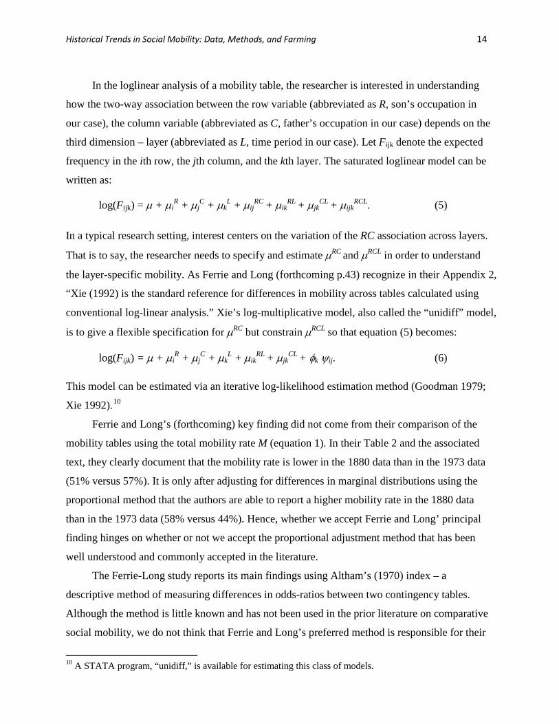
In the loglinear analysis of a mobility table, the researcher is interested in understanding
how the two-way association between the row variable (abbreviated as R, son’s occupation in
our case), the column variable (abbreviated as C, father’s occupation in our case) depends on the
third dimension – layer (abbreviated as L, time period in our case). Let Fijk denote the expected
frequency in the ith row, the jth column, and the kth layer. The saturated loglinear model can be
written as:
log(Fijk) = µ + µiR + µj
C + µkL + µij
RC + µikRL + µjk
CL + µijkRCL. (5)
In a typical research setting, interest centers on the variation of the RC association across layers.
That is to say, the researcher needs to specify and estimate µRC and µRCL in order to understand
the layer-specific mobility. As Ferrie and Long (forthcoming p.43) recognize in their Appendix 2,
“Xie (1992) is the standard reference for differences in mobility across tables calculated using
conventional log-linear analysis.” Xie’s log-multiplicative model, also called the “unidiff” model,
is to give a flexible specification for µRC but constrain µRCL so that equation (5) becomes:
log(Fijk) = µ + µiR + µj
C + µkL + µik
RL + µjkCL + φk ψij. (6)
This model can be estimated via an iterative log-likelihood estimation method (Goodman 1979;
Xie 1992).10
Ferrie and Long’s (forthcoming) key finding did not come from their comparison of the
mobility tables using the total mobility rate M (equation 1). In their Table 2 and the associated
text, they clearly document that the mobility rate is lower in the 1880 data than in the 1973 data
(51% versus 57%). It is only after adjusting for differences in marginal distributions using the
proportional method that the authors are able to report a higher mobility rate in the 1880 data
than in the 1973 data (58% versus 44%). Hence, whether we accept Ferrie and Long’ principal
finding hinges on whether or not we accept the proportional adjustment method that has been
well understood and commonly accepted in the literature.
The Ferrie-Long study reports its main findings using Altham’s (1970) index – a
descriptive method of measuring differences in odds-ratios between two contingency tables.
Although the method is little known and has not been used in the prior literature on comparative
social mobility, we do not think that Ferrie and Long’s preferred method is responsible for their
10 A STATA program, “unidiff,” is available for estimating this class of models.
Historical Trends in Social Mobility: Data, Methods, and Farming 15
surprising conclusion. Indeed, they report a sensitivity analysis using a more conventional
loglinear model of Xie (1992) in Appendix 2, which shows similar, but less pronounced, findings.
This is not surprising, because Altham’s (1970) index is also based on the same idea, as in
loglinear models, that comparing two mobility tables should focus on differences or similarity in
odds-ratios. It is also important to note that Ferrie and Long were able to detect a trend of
declining mobility only if they did not block out diagonal cells. Thus, changes in diagonal cells
representing direct inheritance are of high significance. In their own words, they “cannot…reject
the hypothesis that the associations are identical [for 19th and 20th century US samples] when the
diagonal elements in P and Q are excluded, suggesting that change in the likelihood of direct
inheritance of the father’s occupational status by the son was the greatest difference between
these eras, rather than more subtle change in the structure of association between one
generation’s occupation and that of the next” (Ferrie and Long forthcoming, p. 22).
While the literature on social mobility has long been focused almost exclusively on odds-
ratios, the practice has not gone unchallenged. In particular, Logan (1996) and Hellevik (2007)
have argued that the invariance property of odds-ratios to multiplicative changes in marginal
distributions does not mean in general that they appropriately account for changes in supply and
demand, --- i.e., overall changes in the marginal distribution of occupations. While we are
reluctant to enter the debate on the appropriateness of odds-ratio methods in social mobility
research in general, our examination of the Ferrie-Long data has led us to question the use of
odds-ratios as measures of social mobility for farmers, especially when social mobility is
compared across regimes at very different levels of industrialization, such as the pre-1900 U.S.
and the post-1970 U.S.
THE UNIQUE CASE OF FARMERS
As we discussed before, Ferrie and Long follow the larger literature in defining social
mobility in terms of how close odds-ratios in an observed mobility table are to 1. The case of
perfect mobility is the independence model, in which all observed frequencies are determined
multiplicatively by marginal distributions, shown in equation (2). Lack of mobility, or social
closure, means a deviation from the independence model. To observe concretely how an
observed table departs from the ideal case of perfect mobility, we may take the ratio, cell by cell,
between an observed table and the corresponding table using the same marginal distributions but

Historical Trends in Social Mobility: Data, Methods, and Farming 16
satisfying independence (i.e., equation 2). In Table 3, we present such ratios for two key U.S.
tables in the Ferrie-Long study: one based on the 1860-1880 censuses and one based on the 1973
survey data.
Table 3: Ratios of Observed to Predicted Counts in Two U.S. Mobility Tables
Son's OccupationWhite Collar Farmer
Skilled/ Semiskilled Unskilled
Panel 1. 1860-1880 CensusWhite Collar 2.41 0.72 1.32 0.86Farmer 0.39 1.28 0.51 0.58Skilled/Semiskilled 1.05 0.75 1.68 1.40Unskilled 0.91 0.90 1.00 1.83
Panel 2. 1973 OCGWhite Collar 1.48 0.66 0.90 0.73Farmer 0.14 5.32 0.22 0.42Skilled/Semiskilled 0.56 1.07 1.17 1.27Unskilled 0.63 1.26 1.00 1.42
Father's Occupation
Note: Data are from Tables 1 and 5 of Ferrie and Long (forthcoming). Predicted counts are based on the independence model.
We are immediately drawn to three large outliers (highlighted with shades) in Panel 2, all
pertaining to the social origins of farmers. As ratios of frequencies, all entries in Table 3 are
positive, with 1 as the reference. A number much larger than 1 or much smaller than 1 is thus an
outlier. For Panel 2 (1973 data), the number of farmers with fathers being farmers is far greater
than expected under the independence model (the ratio being 5.3); the numbers of farmers with
fathers being white-collar workers and fathers being skilled and semi-skilled workers are much
smaller than expected (the ratios being 0.14 and 0.22, respectively). While there are clearly
discrepancies between observed and predicted frequencies for Panel 1 (1860-1880 data), we do
not see any discrepancy of a similar magnitude.
We now conduct a few auxiliary analyses to determine if Ferrie and Long’s main finding
of a declining trend in mobility is primarily due to unusually large discrepancies for farmers
between observed data and predicted data under independence in the modern era. First, recall
Ferrie and Long’s own result that the trend is no longer significant when the diagonal cells are
Historical Trends in Social Mobility: Data, Methods, and Farming 17
removed from the analysis. In their comparison of the 1860-1880 and 1973 tables, the log-
likelihood chi-squared statistic (G2) drops from 46.7 with 9 degrees of freedom to 3.2 with 5
degrees of freedom. However, most of this change is driven by a single cell -- farmers with
farmer fathers. If we block this cell from the analysis, the G2 statistic declines to 11.8 with 8
degrees of freedom. Second, when we examine particular odds-ratios that Ferrie and Long
identified as components that contribute the most to the overall d statistic, we immediately notice
the prominence of this diagonal cell of farmers with farmer fathers. As reported by Ferrie and
Long, this cell is involved in all the top seven component odds-ratios that contribute to the d
statistic comparing the 1880 U.S. and the 1973 U.S. (their Table 6).11
d(altered 1973 table, I) = 8.3,
Finally, we carry out an
exercise in which we force the distribution of farmers’ social origin to be the same as the
marginal distribution of all fathers, thus satisfying the independence condition. This alternation
of data involving just one row of data wipes out completely the discrepancy between the 1880
U.S. and the 1973 U.S. using Ferrie and Long’s own method:
d(altered 1880 table, I) = 9.4,
d(altered 1973 table, altered 1880 table) = 6.8.
From these analyses, we conclude that indeed farming was the main source of Ferrie and
Long’s finding of high mobility in the 1880 U.S. as compared to the 1973 U.S. These results are
very similar to Ferrie and Long’s own finding that, after removing cells of inflows to farming
from the analysis, d(P, I)=8.00 and d(Q, I)=8.15, where P is the U.S. 1860-80 mobility table and
Q is the U.S. 1953-73 table, with d(P, Q) = 3.35 (Ferrie and Long forthcoming, pp. 26-27).
However, Ferrie and Long still explicitly dismiss farming as the only source for the higher level
of observed mobility in the 1880 U.S. They state that “the importance of farming by no means
exhausts the sources of higher mobility in the U.S.” (Ferrie and Long forthcoming, pp.19-20).
Let us now recall Ferrie and Long’s main conclusions in their study: (1) social mobility
was higher in the 1880 U.S. than in 1881 Britain; and (2) social mobility was higher in the 1880
U.S. than in the 1973 U.S. These two patterns reported by Ferrie and Long mirror what we know
about the level of industrialization of the two countries at the two time points: the agricultural 11 The same is true for their comparison between the 1880 U.S. and 1881 Britain (their Table 4). Odds-ratios involving the diagonal cell of farmers with farmer fathers are often unusually large. For example, the odds-ratio that involves the first two rows and first two columns of the 1973 U.S. table is 84 (top row of their Table 6).
Historical Trends in Social Mobility: Data, Methods, and Farming 18
sector of the U.S. labor force was still large (around 50%) in 1880 but became very small (under
3%) in 1973, whereas the British labor force was overwhelmingly non-agricultural by 1881.
Ferrie and Long also entertained the rapid reduction in the farming sector in the U.S. as an
explanation for their observed decline in social mobility in the U.S. but rejected the hypothesis.
Their discussion mostly focuses on selectivity of farmers. We also consider this hypothesis, and
our consideration of the hypothesis leads us to challenge a basic premise that underlies the
method used by Ferrie and Long and indeed almost all other researchers studying comparative
social mobility.
To clarify our argument, let us examine Table 4, where we present descriptive statistics
about farmers in six U.S. datasets (ranked in a chronological order). We observe a steady and
rapid reduction of the share of farmers in the labor force, from 51% in the 1850-1880 census
dataset to just over 1% in the 1979 NLSY data.12
Farming is a unique occupation in contemporary society in a number of aspects. First, in
any developed nation, it has gone through a very rapid reduction as a share of the economy
during industrialization. Second, in studies of occupational prestige, farming is generally lowly
ranked (Treiman 1977).
This societal change in the reduction of the
farming labor force has been very large in scale. It also means that, structurally, many sons of
fathers who were farmers had to leave the farm (Blau and Duncan 1967). This structural force is
further exacerbated by the fact that farmers tend to have more children than non-farmers
(Duncan 1966).
13
Third, farming is one of these few occupations where direct
inheritance from father to son was normative in the past and still widely practiced today. For
these reasons, we argue that it should be treated differently from other occupations. While it may
be sensible to expect a cell in a mobility table to rise or fall as a function of marginal
distributions, as shown in equation (2), under perfect mobility, it may be incorrect however to
apply the proportionality principle to the case of farmers. The uniqueness of farmers was
observed long ago by Duncan (1966, p.68), who remarked that “[farming] is probably an
extreme example of an occupation recruited from sons of men pursuing the same occupation.”
12 Note that the NLSY study began in 1979 when the subjects were young (14-22 years old). Ferrie and Long’s mobility table from the NLSY pertains to jobs held by the subjects in years later than 1979. 13 Farming consists of farm owners and farm workers, with the former much more highly ranked in prestige than the latter.

Historical Trends in Social Mobility: Data, Methods, and Farming 19
Table 4: Farmers' Share in Labor Force and Relative Family Origin in the U.S., by Data Source
White Collar FarmerSkilled/
Semiskilled UnskilledCensus 1850-1880Marginal 7.1% 68.3% 18.1% 6.4%Farmers 50.9% 4.3% 83.3% 9.0% 3.4%
Census 1860-1880Marginal 9.5% 64.1% 17.4% 9.0%Farmers 43.9% 3.7% 82.2% 8.9% 5.2%
Census 1880-1900Marginal 11.3% 56.5% 21.5% 10.7%Farmers 31.5% 3.4% 83.7% 7.4% 5.5%
OCG 1973Marginal 27.9% 15.1% 41.4% 15.6%Farmers 2.5% 3.9% 80.3% 9.2% 6.6%
GSS 1977-1990Marginal 38.6% 9.1% 41.9% 10.4%Farmers 1.7% 0.0% 86.7% 6.7% 6.7%
NSLY 1979Marginal 43.5% 3.5% 43.3% 9.8%Farmers 1.3% 7.7% 61.5% 15.4% 15.4%Note: Data were provided by Joseph Ferrie. See Ferrie and Long (forthcoming).
By Father's OccupationShare of Labor Force
As America became more and more industrialized, we know that large proportions of famers’ sons migrated out of farming (Blau and Duncan 1967). With time, the proportion of sons with farmer fathers necessarily became smaller and smaller. This is apparent in Ferrie and Long’s data, shown in the rows labeled “marginal” for each data set in Table 4: the percentage of farmer farmers among all workers declines rapidly from 68% in the 1850-1880 data to 15% in the 1973 data, and further to under 4% in the 1979 NLSY data. If the independence model were true, we would expect the inflow distribution of farmers to mirror that of the “marginal.” However, the independence assumption is strongly violated: the steady and rapid decline in the proportion of farmer fathers in general did not translate into a parallel decline in the proportion of farmer fathers among farmers, shown in the rows labeled “farmers” in Table 4. In fact, the distribution of father’s occupation among farmers remains stable across all the American datasets

Historical Trends in Social Mobility: Data, Methods, and Farming 20
in the Ferrie and Long study.14 It does not matter how fathers’ occupation is distributed overall; the majority of fathers among farmers (around 80% for almost all datasets) have always remained farmers.15
In their classic study, Blau and Duncan (1967, p.60) recognized the uniqueness of farmers, as they drew “a boundary between the industrial and the agricultural sectors of the labor force, which is manifest in the finding that both intergenerational and intragenerational movements from any nonfarm occupation to either of the two farm groups fall short of what would be expected under conditions of statistical independence.” Building on Blau and Duncan’s observation, economists Laband and Lentz (1983) provided an explanation using human capital theory: a son accumulates valuable human capital, both about farming in general and about particular soil farmed by his father while growing up on the farm. To prove their theoretical explanation, Laband and Lentz showed empirical evidence that farmers who had farmer fathers “earned a premium for the added experience they have over [their counterparts who did not have farmer fathers]” (p.314).
Based on the insights of Duncan (1966), Blau and Duncan (1967), and Laband and Lentz (1983), as well as the empirical pattern shown in Table 4, we thus propose that farmers are unique in that they overwhelmingly come from farmer families, regardless of secular changes in the overall occupational structure. Of course this uniqueness can be sustained only when the agricultural sector is shrinking or at least not growing. If our proposition is taken to be true, then the declining trend of mobility from the 19th century to contemporary America that is reported by Ferrie and Long is simply an artifact of their statistical method of relying on the independence model as the reference and the proportional adjustment for differences in marginal distributions. That is, their measure of mobility merely captures the discrepancy of the conditional distribution of farmers’ fathers from the marginal distribution of all fathers. Over time, the two distributions grow more and more dissimilar. We believe that this trend of growing dissimilarity over time is due to two separate social forces: on the one hand, industrialization diminishes the demand for farmers, but on the other hand, farming is such a unique occupation that the dominant inflow of farmers has remained to be of farmer origin. Ferrie and Long misidentified this trend of growing dissimilarity as a declining trend in social mobility.
14 Indeed, it is roughly the same across many other datasets we have examined for this paper. However, to ensure comparability across datasets and to save space, we only present the results for the U.S. datasets used in the Ferrie-Long study. 15 This is a unique feature pertaining only to farmers. For example, we repeated the same analysis for unskilled workers and did not find the dominance of fathers in the same occupation to be true throughout the datasets.

Historical Trends in Social Mobility: Data, Methods, and Farming 21
CONCLUSION We congratulate Ferrie and Long on their significant contribution to an already large literature on comparative social mobility. Using data from linked historical censuses, the Ferrie-Long study has provided, for the first time, nationally representative data on social mobility in the 19th century U.S. and Britain. The valuable historical data allow them, as well as other scholars in the future, to examine long-term trends in social mobility and to compare mobility regimes across countries in a distant past. A key finding of the Ferrie-Long study is that, compared to either today’s U.S. or Britain at the same time, the pre-1900 U.S. exhibited an unusually high level of social mobility. While we applaud the Ferrie-Long study for providing good historical data and for making a bold statement about the “good old days” for social mobility in America’s past, we caution the reader not to accept the study’s main conclusion yet. In this paper, we have discussed three sets of issues. First, the data quality of the Ferrie-Long study is far more limiting than the authors acknowledge. For example, they did not report the fact that mobility is impossible to construct for almost a third of their subjects because they did not co-reside with their fathers at the time of an earlier census. Furthermore, through an analysis of data that were overlooked by Long and Ferrie, we found suggestive evidence that the likelihood of matching is selective with respect to mobility in a way that is favorable to their conclusion.
Second, Ferrie and Long’s key finding hinges on an operationalization of the concept of “social mobility” in terms of odds-ratios and the inclusion of diagonal cells, manifested in results using Altham’s index for whole tables. It is true that the standard literature in sociology on comparative social mobility is also almost entirely concerned with odds-ratios as measures of relative social mobility through the use of the loglinear model. However, the loglinear approach, as commonly practiced, differs in one important respect:16
16 Another difference is that a loglinear model smoothes observed data through modeling and thus minimizes the influences of sampling errors, whereas Altham’s index treats sampled data as if they were population data.
diagonal cells are often blocked out in loglinear models of mobility tables so that attention is focused only on independence for off-diagonal cells (called “quasi-independence”), whereas Ferrie and Long’s main analysis includes diagonal cells. Although the method of blocking diagonal cells in loglinear analysis was not designed specifically to handle the unique case of farmers, who seem to defy the independence hypothesis in terms of being proportional to marginal distributions, it is fortuitous that this practice effectively removes the confounding influence of the uniqueness of farmers in comparative studies of social mobility in past research.

Historical Trends in Social Mobility: Data, Methods, and Farming 22
Third, the shortcoming of an exclusive reliance on odds-ratios becomes apparent when we look at farmers. Since 1880, the agricultural sector of the U.S. labor force has rapidly shrunk. Corresponding to this trend is a secular decline in the proportion of farmers among fathers of all workers. In the odds-ratio approach, perfect mobility means independence, which in term dictates that the likelihood of drawing workers in any occupation, even farmers, from farmer origin should decline accordingly. However, we have argued and shown in this paper that farmers are unique in always drawing their members overwhelmingly from farmer origins, regardless of secular changes in the overall occupational structure. As a result of these two separate social forces, the distribution of father’s occupation among farmers became more and more dissimilar to that of the distribution of father’s occupation among all workers. Ferrie and Long’s finding of a significant decline in social mobility merely reflects this trend of growing disparity between farmers and other workers in terms of their father’s occupation.
If Ferrie and Long’s key finding is no more than a methodological artifact, why have so many other researchers in the loglinear tradition missed it? Additional to the lack of long-term trend data in the past, another important reason is that the loglinear model is both too powerful and at the same time too complicated. The power of the loglinear model lies in its ability to fit any observed data with flexible parameterization. In particular, researchers are often quick in fitting diagonal cells to block out immobility when their models do not fit observed data. As we showed earlier, and as Ferrie and Long explained, diagonal cells do carry useful information and do matter. We would not have learned as much as we did from Tables 3 and 4, if we had excluded diagonal cells early on. Much of the uniqueness of farmers has to do with a diagonal cell: farmers from farmer origins. To make the loglinear model powerful in explaining observed data well, researchers often fit many parameters but do not always exercise care in interpreting them. It was only through applying Ferrie and Long’s simple and descriptive approach that we arrived at the conjecture that farmers may be qualitatively distinct from other workers in keeping their social origin distribution constant over time. Proposed as an alternative explanation of Ferrie and Long’s key finding, our conjecture is still a hypothesis. We welcome other researchers to debate and evaluate our hypothesis in future studies.

Historical Trends in Social Mobility: Data, Methods, and Farming 23
REFERENCES
Altham, P.M. 1970. “The Measurement of Association of Rows and Columns for an r × s Contingency Table.” Journal of the Royal Statistical Society, Series B, 32: 63-73.
Angrist, Joshua. D. and Alan. Krueger. 1999. "Empirical Strategies in Labor Economics." Pp. 1277-366 in Handbook of Labor Economics, vol. 3A, edited by O. Ashenfelter and D.Card. Amsterdam: Elsevier.
Blau, Peter M. and Otis Dudley Duncan. 1967. The American Occupational Structure. New York: Wiley.
Breen, Richard and Jan O. Jonsson. 2007. “Explaining Change in Social Fluidity: Educational Equalization and Educational Expansion in Twentieth-Century Sweden.” American Journal of Sociology 112: 1775-1810.
Duncan, Otis Dudley. 1966. “Methodological Issues in the Analysis of Social Mobility.” Pp. 51-97 inSocial Structure and Mobility in Economic Development, edited by N.J. Smelser and S.M. Lipset. Chicago: Aldine.
Erikson, Robert and John H. Goldthorpe. 1992. The Constant Flux: A Study of Class Mobility in Industrial Societies. Oxford, England: Clarendon.
Featherman, David L., F. Lancaster Jones, and Robert M. Hauser. 1975. "Assumptions of Social Mobility Research in the US: The Case of Occupational Status." Social Science Research 4:329-360.
Featherman, David L. and Robert M. Hauser. 1978. Opportunity and Change. New York: Academic Press.
Ferrie, Joseph, and XXX Long. Forthcoming. “Intergenerational Occupational Mobility in Britain and the U.S. Since 1850.” American Economic Review XX.
Ganzeboom, Harry B. G. , Donald J. Treiman, Wout C. Ultee. 1991. “Comparative Intergenerational Stratification Research: Three Generations and Beyond.” Annual Review of Sociology 17:277-302.
Goodman, Leo A. 1972. “Some Multiplicative Models for the Analysis of Cross-Classified Data.” Pp. 649-696 in Proceedings of the Sixth Berkeley Symposium on Mathematical Statistics and Probability, edited by L. LeCam et al., University of California Press, Berkeley. Also in Goodman, Leo. 1984. The Analysis of Cross-Classified Data Having Ordered Categories. Cambridge, MA: Harvard University Press.
Goodman, Leo A. 1979. "Simple Models for the Analysis of Association in Cross-Classifications Having Ordered Categories." Journal of the American Statistical Association 74:537-552. Also in Goodman, Leo. 1984. The Analysis of Cross-Classified Data Having Ordered Categories. Cambridge, MA: Harvard University Press.
Grusky, David. 1986. “American Social Mobility in the 19th and 20th Centuries.” University of Wisconsin Center for Demography and Ecology Working Paper 86-28.
Grusky, David B. and Robert M. Hauser. 1984. “Comparative Social Mobility Revisited: Models of Convergence and Divergence in 16 Countries.” American Sociological Review 49: 19-38.
Grusky, David B., and Jesper B. Sørensen. 1998. “Can Class Analysis Be Salvaged?” American Journal of Sociology 103, pp. 1187-1234.
Guest, Avery M., Nancy S. Landale, and James C. McCann. 1989. “Intergenerational Mobility in the Late 19th Century United States.” Social Forces 68: 351-378.
Hauser, Robert M. 1978. “A Structural Model of the Mobility Table,” Social Forces 56:919-953.

Historical Trends in Social Mobility: Data, Methods, and Farming 24
Hauser, Robert M., John N. Koffel, Harry P. Travis, Peter J. Dickinson. 1975. “Temporal Change in Occupational Mobility: Evidence for Men in the United States.” American Sociological Review 40:279-297.
Hellevik, Ottar. 2007. “‘Margin Insensitivity’ and the Analysis of Educational Inequality.” Czech Sociological Review 43:1095 -1119.
Hout, Michael. 1988. "More Universalism, Less Structural Mobility: The American Occupational Structure in the 1980s." American Journal of Sociology 93:1358-1400.
Laband, David N. and Bernard F. Lentz. 1983. “Occupational Inheritance in Agriculture.” American Journal of Agricultural Economics 65: 311-314.
Lipset, Seymour Martin and Reinhard Bendix. 1964. Social Mobility in Industrial Society. Berkeley: University of California Press.
Logan, John Allen. 1996. “Rules of Access and Shifts in Demand: A Comparison of Log-Linear and Two-Sided Logit Models.” Social Science Research 25: 174-199.
Manski, Charles. 1995. Identification Problems in the Social Sciences. Cambridge, MA: Harvard University Press.
Powers, Daniel A. and Yu Xie. 2008. Statistical Methods for Categorical Data Analysis, Second Edition. Howard House, England: Emerald.
Ruggles, Steven, Matthew Sobek, Trent Alexander, Catherine A. Fitch, Ronald Goeken, Patricia Kelly Hall, Miriam King, and Chad Ronnander. 2009. Integrated Public Use Microdata Series: Version 4.0 [Machine-readable database]. Minneapolis, MN: Minnesota Population Center [producer and distributor]. http://usa.ipums.org/usa/
Sobel, Michael E., Michael Hout and Otis Dudley Duncan. 1985. “Exchange, Structure, and Symmetry in Occupational Mobility.” American Journal of Sociology 91:359-372.
Treiman, Donald. 1977. Occupational Prestige in Comparative Perspective. New York: Academic Press.
Vallet, Louis-André. 2001. “Forty Years of Social Mobility in France.” Revue française de sociologie. 42: 5-64, supplement.
Xie, Yu. 1992. “The Log-Multiplicative Layer Effect Model for Comparing Mobility Tables.” American Sociological Review 57:380-395.