151© WILDLIFE BIOLOGY · 12:2 (2006)

Historical changes in black brant Branta bernicla nigricans use on Humboldt Bay, California

Jeffrey E. Moore & Jeffrey M. Black

Moore, J.E. & Black, J.M. 2006: Historical changes in black brant Branta ber-nicla nigricans use on Humboldt Bay, California. - Wildl. Biol. 12: 151-162.

We examined 70 years (1931-2000) of black brant Branta bernicla nigricans abundance on Humboldt Bay, California. We used linear regression to convert count data to a standard variable (use-days) for evaluating hypotheses that explain temporal trends in brant use. Winter and spring brant-days on Humboldt Bay declined sharply in the mid-1950s and continued to decline through the mid-1980s, but have since increased. Evidence suggests that this trend may have been driven largely by changes in temporal patterns of hunting pressure on Hum-boldt Bay. We found little convincing support for alternative hypotheses such as changes in eelgrass Zostera marina condition over time, effects of non-hunt-ing disturbance, and correlation with trends in abundance at the flyway level. Our study affirms the appropriateness of current hunting regulations for brant in California, but poses a challenge to wildlife managers who wish to provide hunting opportunities without displacing brant from important staging and win-tering areas.

Key words: abundance, Branta bernicla nigricans, distribution, disturbance, eelgrass, hunting, Zostera marina

Jeffrey E. Moore* & Jeffrey M. Black, Waterfowl Ecology Research Group, Humboldt State University, Arcata, CA 95521, USA - e-mail addresses: jemoore @duke.edu (Jeffrey E. Moore); jmb7002@humboldt.edu (Jeffrey M. Black)

*Present address: Duke Center for Marine Conservation, Duke University, 135 Duke Marine Lab Road, Beaufort, NC 28516, USA

Corresponding author: Jeffrey E. Moore

Received 16 June 2004, accepted 27 January 2005

Associate Editor: Anthony D. Fox

During spring migration, black brant Branta bernicla nigricans (in the following referred to as 'brant') feed on eelgrass Zostera marina in shallow bays and estuaries along west coast North America (Reed et al. 1998b, Moore et al. 2004), where they accumulate nutrient reserves critical for successful reproduction (Ankney 1984, Ebbinge & Spaans 1995). Humboldt Bay is the most important spring staging area in California based on peak use data, and the fourth most important site in the Pacific flyway (Moore et al. 2004). Lee (2001) esti-mated that approximately 60% of the flyway population used the bay in spring 2001, probably because of its high

eelgrass abundance and relative isolation from other staging areas (Moore et al. 2004). Our goals in this paper are to: 1) use historic counts to describe trends in brant use of Humboldt Bay, 2) evaluate use-patterns in relation to variation in hunting disturbance or Pacific flyway pop-ulation trends, and 3) recommend an annual protocol for monitoring brant use.

Single winter censuses for Humboldt Bay have been conducted since 1931, with more frequent fall-, winter- and spring-counts since the 1970s. Data indicate that win-ter and spring brant use declined suddenly in the mid-1950s, continued to decrease through the mid-1980s, and

14368 WB2_2006-v3.indd 151 13/06/06 10:31:58

152 © WILDLIFE BIOLOGY · 12:2 (2006)

then increased through 2000. Midwinter survey data reveal similar declines at winter and spring sites in Oregon and Washington (Drut & Trost 2000). Proposed hypoth-eses to explain changes in brant use primarily include disturbance due to hunting and other human factors and eelgrass habitat degradation (Einarsen 1965, Smith & Jen- sen 1970, Henry 1980, Subcommittee on Pacific Brant 1992). Investigation of these hypotheses has been hamper-ed, however, by the sporadic nature and inconsistent tim-ing of surveys, and lack of historical data for eelgrass condition or non-hunting human disturbance. We found predictive relationships between seasonal use-day esti-mates and count data, thus enabling us to recreate a his-torical record of brant use-days on Humboldt Bay that could be used to empirically test two possible hypotheses concerning use at a key staging area.

Material and methods

Study areaHumboldt Bay, located on the northern California coast, is the second largest estuary in the state, with a water surface area of 62.4 km2 at mean high water (MHW; Proctor et al. 1980). The bay has three main sections, two of which receive 99% of the bay’s brant use, i.e. Arcata Bay and South Bay. These areas consist of exten-sive tidal flats, accounting for 65-70% of the total MHW area of the bay (Barnhart et al. 1992). Eelgrass, which varies in extent annually, occurs below about +0.3 to +0.4 m (relative to mean lower low water; MLLW). In 1997, eelgrass covered approximately 1,044 ha of which 309 ha were in Arcata Bay and 720 ha were in South Bay (Terra-Mar 1997). A long narrow channel (Arcata Channel) connecting two sections of the bay contains about 15 ha of eelgrass, and supports about 1% of annu-al brant use (Humboldt Bay National Wildlife Refuge (HBNWR), unpubl. data). Shoot and biomass densities are also consistently higher on South Bay than on Arcata Bay, where an estimated 78-90% of the total biomass occurs (Keller 1963, Waddell 1964, Harding & Butler 1979, Bixler 1982).

Sources of brant abundance data Moffitt (1931-1941, 1943) conducted annual February brant surveys along the entire coast of California during 1931-1942. We used U.S. Fish and Wildlife Service (USFWS) mid-winter survey data for 1940-1974. Mid-winter counts were usually conducted in January; how-ever some were as late as February or March (Henry 1980; Marty Drut, USFWS, pers. comm.). We obtained addi-tional count data from Bentley & Christianson (1957,

cited in Henry 1980), Denson (1961), Denson & Murrell (1962), and Monroe (1973, cited in Henry 1980). During 1975-1978, Henry (1980) conducted weekly counts of brant on Humboldt Bay during fall, winter and spring, and estimated weekly, monthly and seasonal brant use (i.e. number of brant use-days). Since 1978, USFWS personnel at HBNWR used this protocol to continue the surveys. Except for USFWS mid-winter aerial surveys, counts were ground based.

Analysis of winter and spring brant useTwo factors made it impossible to directly compare all brant data. First, while data from 1975-2000 provided direct estimates of seasonal brant use-days, surveys in many of those years occurred on South Bay only (Table 1). We estimated total Humboldt Bay use-days in these years by dividing use on South Bay by 0.83, as this was the average proportion of total use that occurred on South Bay in 11 years between 1975 and 2000 (range: 0.78-0.94; Moore et al. 2004).

Secondly, data prior to 1975 typically consisted of 1-4 counts during winter or spring, but they have not been used to estimate seasonal use-days. We used linear re-gression on South Bay data during 1975-2000 (N = 24 years) to identify predictive relationships between indi-vidual counts conducted at different times during win-ter and spring, with seasonal and total use-days in the same year. For example, we examined whether a single count conducted in the second week of February (as per Moffitt’s protocol through the 1930s) could predict the estimate of use-days occurring in the same winter or spring. If a strong relationship existed, we extrapolated pre-1975 winter or spring brant use-days by entering available count values into a regression equation with slope coefficients that were estimated using the post-1975 data. We defined a strong relationship to be the regressions in which > 50% of the variation in use-days was explained by count data (i.e. adjusted R2 > 0.50). Presumably, we could have used a slightly different cut-off (e.g. R2 > 0.40 or 0.60) with similar results. We defined winter use as that occurring during January and February, and spring use as that occurring from March through May. We excluded December in winter use-day estimates because: 1) several of the years used to iden-tify regression relationships (1975-2000) contained no December data, 2) pre-1975 December counts provid-ed little additional predictive power to estimate winter use-days because they were conducted in years when both January and/or February were also counted, 3) it is not clear from historical counts whether brant in December were late-fall migrants, winter residents or early-spring migrants, and 4) relative to brant numbers in January

14368 WB2_2006-v3.indd 152 13/06/06 10:31:58

153© WILDLIFE BIOLOGY · 12:2 (2006)

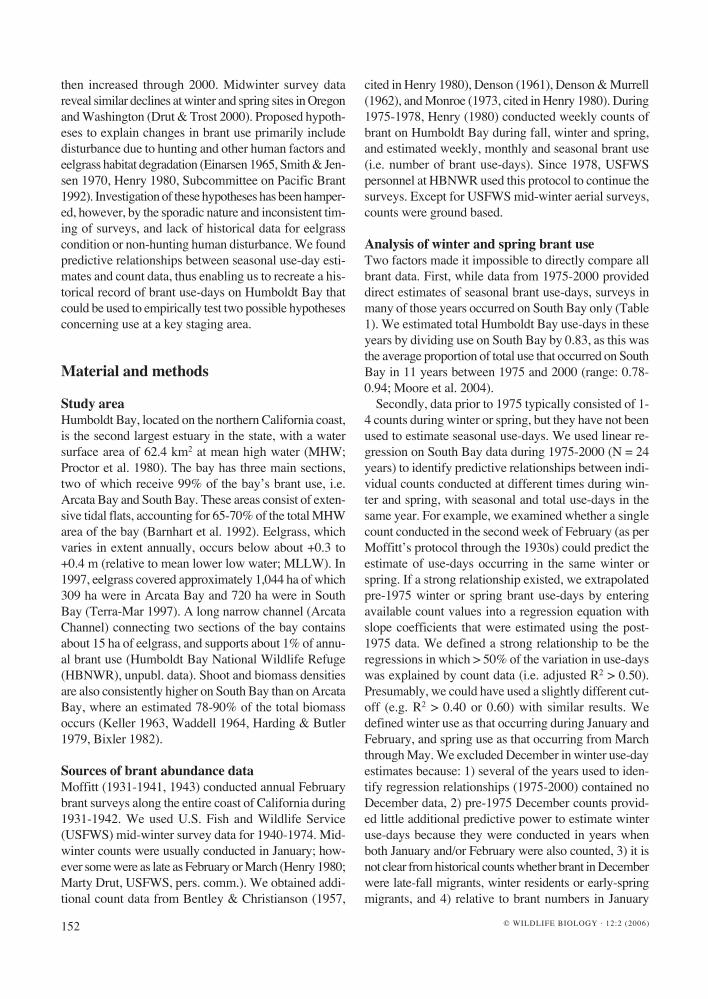
Table 1. Individual counts of black brant during winter and spring on Humboldt Bay (Arcata and South bays). In months when multiple counts were conducted, the peak count is reported.

Year December January February March April May Source1930/31 4200 Moffitt 19311931/32 3000 29415 Moffitt 19321932/33 5000 13000 3000 Moffitt 19331933/34 10000 16860 Moffitt 19341934/35 2000 105000 Moffitt 19351935/36 50000 Moffitt 19361936/37 22500 30000 Moffitt 19371937/38 45000 100000 Moffitt 19381938/39 29000 100000 25000 Moffitt 19391939/40 15385 56375 Moffitt 19401940/41 16300 50000 Moffitt 19411941/42 20000 48000 Moffitt 19431942/43 8000 USFWS winter survey1943/44 2500 USFWS winter survey1944/45 16000 USFWS winter survey1945/46 USFWS winter survey1946/47 25000 USFWS winter survey1947/48 27120 USFWS winter survey1948/49 27505 USFWS winter survey1949/50 32500 USFWS winter survey1950/51 36000 USFWS winter survey1951/52 25000 USFWS winter survey1952/53 28000 USFWS winter survey1953/54 7500 USFWS winter survey1954/55 11870 USFWS winter survey1955/56 7000 19010 USFWS winter survey1956/57 1700 6900 18800 37000 25000 Denson & Bentley 1962

Denson & Murrell 19621957/58 57 11300 Denson & Murrell 19621958/59 113 4850 Denson & Murrell 19621959/60 100 62 10000 35000 30000 300 Denson 1961

Denson & Murrell 19621960/61 600 2000 15000 40000 40000 30000 Denson 1961,

Denson & Murrell 19621961/62 55800 USFWS winter survey1962/63 383 USFWS winter survey1963/64 2695 USFWS winter survey1964/65 1 USFWS winter survey1965/66 0 USFWS winter survey1966/67 0 USFWS winter survey1967/68 38 0 420 10900 39140 44 Monroe 19731968/69 0 6 0 12700 13425 900 Monroe 19731969/70 0 47 1170 12600 11000 400 Monroe 19731970/71 0 USFWS winter survey1971/72 0 USFWS winter survey1972/73 0 200 12000 33600 10500 HBNWR survey1973/74 0 USFWS winter survey1974/75a 7 3000 15000 37500 1200 Henry 19801975/76 80 140 4375 16810 22275 463 Henry 19801976/77 46 70 2760 21628 18030 692 Henry 19801977/78a 80 150 2500 20950 11680 950 Henry 19801978/79a 7 52 185 17250 20580 463 HBNWR survey1979/80a 60 49 1295 15270 11760 901 HBNWR survey1980/81a 400 59 1203 8880 11080 1340 HBNWR survey1981/82a 57 80 1025 10860 5050 1430 HBNWR survey1982/83a 37 30 450 6100 13450 250 HBNWR survey1983/84a 18 201 490 10100 7000 615 HBNWR survey

.. continued on the next page

14368 WB2_2006-v3.indd 153 13/06/06 10:31:59

154 © WILDLIFE BIOLOGY · 12:2 (2006)

and February, numbers in December have been low since the mid-1950s (see Table 1), and were typically low before 1975 also (Moffitt 1932, 1935, 1936); therefore, December use-days probably contributed relatively little to the number of use-days each year.

Different regression models were used to estimate brant use-days in different years, with independent vari-ables defined by the dates for which pre-1975 count data were available (Appendix I). To estimate use-days from Moffitt’s data in the 1930s and 1940s, our independent variable was the number of brant recorded during the second week of February. If only monthly peak num-bers were reported in a particular pre-1975 year, we de-scribed the relationship between monthly peak counts and brant use-days in post-1975 years. In some instances, we did not know the exact date on which a pre-1975 count was conducted, nor whether it was a peak esti-mate. So, we assumed that such a count was a peak esti-mate if it exceeded peak values in post-1975 years. When the number of brant on a pre-1975 survey equaled zero, and we only knew which month the survey was conduct-ed, we assumed this count was from the first week of the month, when numbers would be at their lowest (zero-counts were always from January or February). When multiple counts were available to predict use-days in a particular pre-1975 year, we used stepwise regression to select the combinations of counts that produced the best predictive model (i.e. that which maximized the adjusted R2).

Once we had estimated historical brant use-days for each year, we used linear regression to determine wheth-er annual variation on Humboldt Bay corresponded with

the historical timing of hunting seasons or annual har-vest estimates based on post hunting-season interviews with hunters (M. Drut, pers. comm., California Depart-ment of Fish and Game, unpubl. data). We also used re-gression to investigate whether annual trends in brant use-days on Humboldt Bay correlated with annual Pa-cific flyway population estimates (Drut & Trost 2000).

Analysis of fall brant useSingle counts were conducted on Humboldt Bay during fall migration (October-November) in seven years dur-ing 1956-1975. Weekly counts were used to estimate brant use-days on South Bay in 17 years during 1976-2000. We estimated bay-wide use (Arcata Bay and South Bay combined) in years following 1975 by dividing use-days on South Bay by 0.96, since the average percent-age-use for that area ranged within 94-97% in fall (HBNWR, unpubl. data). Using the same methods as for winter and spring data, we identified linear relationships between fall use-days and peak counts from October and November in post-1975 data, from which we estimated fall use-days for the seven years prior to 1975 (Adjusted R2 = 0.62, F2,13 = 13.17, P < 0.001). We used a Mann-Whitney test to examine whether fall use-days were low-er in years when hunting seasons took place in fall.

Results

Winter and spring brant useStrong relationships existed between estimates of winter brant use-days and individual brant counts conducted in

Year December January February March April May Source1984/85a 25 50 2076 5200 7386 1060 HBNWR survey1985/861986/87a 43 86 600 4255 12460 400 HBNWR survey1987/88a 109 161 3000 8000 8390 508 HBNWR survey1988/891989/90a 50 500 3400 10095 16375 5823 HBNWR survey1990/91a 123 750 1638 12380 10095 2070 HBNWR survey1991/92b 2000 9050 24710 24720 3757 HBNWR survey1992/93b 3950 10660 23755 18415 2655 HBNWR survey1993/94b 4100 11535 31870 26530 585 HBNWR survey1994/95b 5825 20570 19504 24053 HBNWR survey1995/96b 580 5094 19281 19605 16043 2373 HBNWR survey1996/97b 334 6636 12319 14683 11561 1452 HBNWR survey1997/98c 9119 10300 31400 14853 6300 HBNWR survey1998/99b 4368 17812 23412 19406 474 HBNWR survey1999/2000b 1144 6220 18490 24455 15330 2715 HBNWR survey

a Counts include brant on South Bay only.b Counts also include the Arcata Channel.c Counts also include brant in pastures surrounding Humboldt Bay.

... Table 1 continued

14368 WB2_2006-v3.indd 154 13/06/06 10:31:59

155© WILDLIFE BIOLOGY · 12:2 (2006)

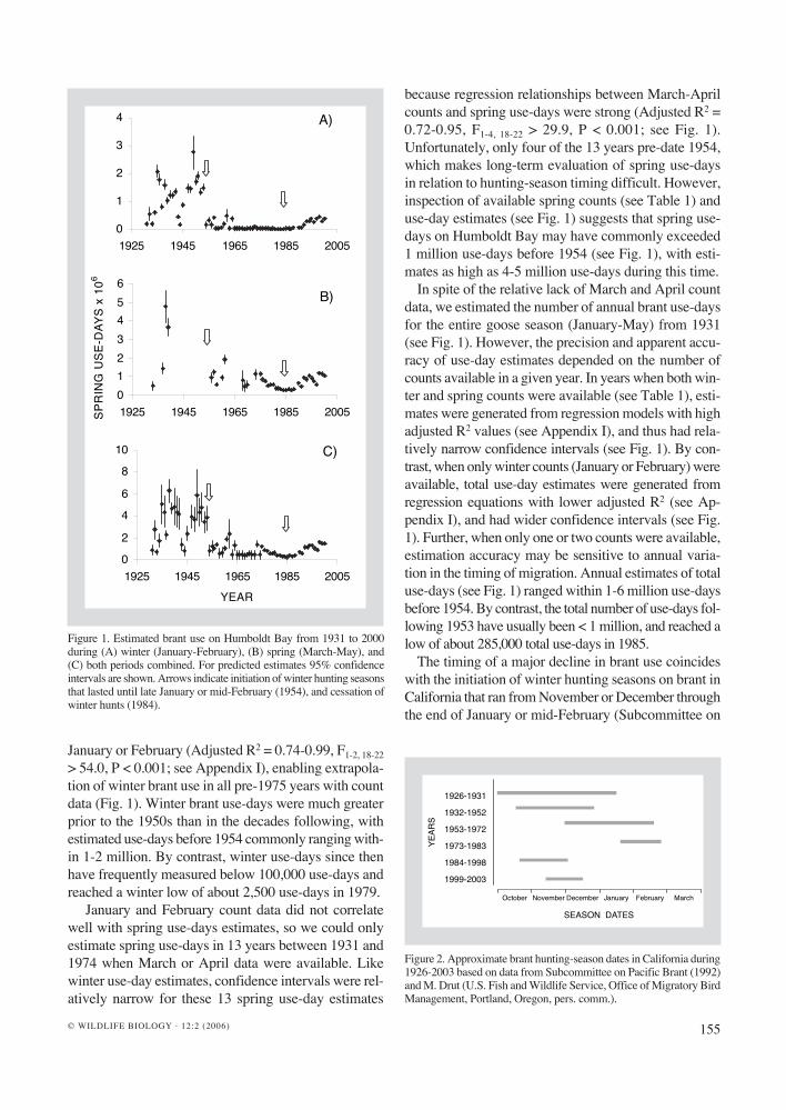
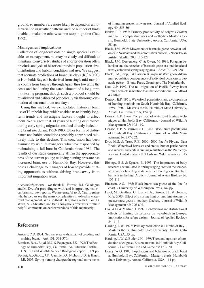
January or February (Adjusted R2 = 0.74-0.99, F1-2, 18-22 > 54.0, P < 0.001; see Appendix I), enabling extrapola-tion of winter brant use in all pre-1975 years with count data (Fig. 1). Winter brant use-days were much greater prior to the 1950s than in the decades following, with estimated use-days before 1954 commonly ranging with-in 1-2 million. By contrast, winter use-days since then have frequently measured below 100,000 use-days and reached a winter low of about 2,500 use-days in 1979.

January and February count data did not correlate well with spring use-days estimates, so we could only estimate spring use-days in 13 years between 1931 and 1974 when March or April data were available. Like winter use-day estimates, confidence intervals were rel-atively narrow for these 13 spring use-day estimates

because regression relationships between March-April counts and spring use-days were strong (Adjusted R2 = 0.72-0.95, F1-4, 18-22 > 29.9, P < 0.001; see Fig. 1). Unfortunately, only four of the 13 years pre-date 1954, which makes long-term evaluation of spring use-days in relation to hunting-season timing difficult. However, inspection of available spring counts (see Table 1) and use-day estimates (see Fig. 1) suggests that spring use-days on Humboldt Bay may have commonly exceeded 1 million use-days before 1954 (see Fig. 1), with esti-mates as high as 4-5 million use-days during this time.

In spite of the relative lack of March and April count data, we estimated the number of annual brant use-days for the entire goose season (January-May) from 1931 (see Fig. 1). However, the precision and apparent accu-racy of use-day estimates depended on the number of counts available in a given year. In years when both win-ter and spring counts were available (see Table 1), esti-mates were generated from regression models with high adjusted R2 values (see Appendix I), and thus had rela-tively narrow confidence intervals (see Fig. 1). By con-trast, when only winter counts (January or February) were available, total use-day estimates were generated from regression equations with lower adjusted R2 (see Ap-pendix I), and had wider confidence intervals (see Fig. 1). Further, when only one or two counts were available, estimation accuracy may be sensitive to annual varia-tion in the timing of migration. Annual estimates of total use-days (see Fig. 1) ranged within 1-6 million use-days before 1954. By contrast, the total number of use-days fol-lowing 1953 have usually been < 1 million, and reached a low of about 285,000 total use-days in 1985.

The timing of a major decline in brant use coincides with the initiation of winter hunting seasons on brant in California that ran from November or December through the end of January or mid-February (Subcommittee on

SPR

ING

USE

-DAY

S x

106

0

1

2

3

4

1925 1945 1965 1985 2005

A)

0123456

1925 1945 1965 1985 2005

B)

0

2

4

6

8

10

1925 1945 1965 1985 2005YEAR

C)

Figure 1. Estimated brant use on Humboldt Bay from 1931 to 2000 during (A) winter (January-February), (B) spring (March-May), and (C) both periods combined. For predicted estimates 95% confidence intervals are shown. Arrows indicate initiation of winter hunting seasons that lasted until late January or mid-February (1954), and cessation of winter hunts (1984).

SEASON DATES

1926-1931

1932-1952

1953-1972

1973-1983

1984-1998

1999-2003

October November December January February March

YEAR

S

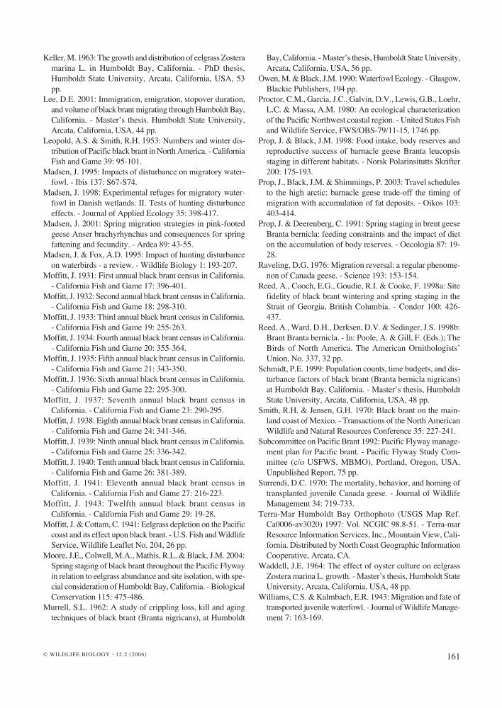
Figure 2. Approximate brant hunting-season dates in California during 1926-2003 based on data from Subcommittee on Pacific Brant (1992) and M. Drut (U.S. Fish and Wildlife Service, Office of Migratory Bird Management, Portland, Oregon, pers. comm.).

14368 WB2_2006-v3.indd 155 13/06/06 10:32:00

156 © WILDLIFE BIOLOGY · 12:2 (2006)

Pacific Brant 1992). Prior to 1953, hunting seasons usu-ally ran from October or November through mid to late December, although they did occasionally run through the first week of January, and until 20 January in 1946

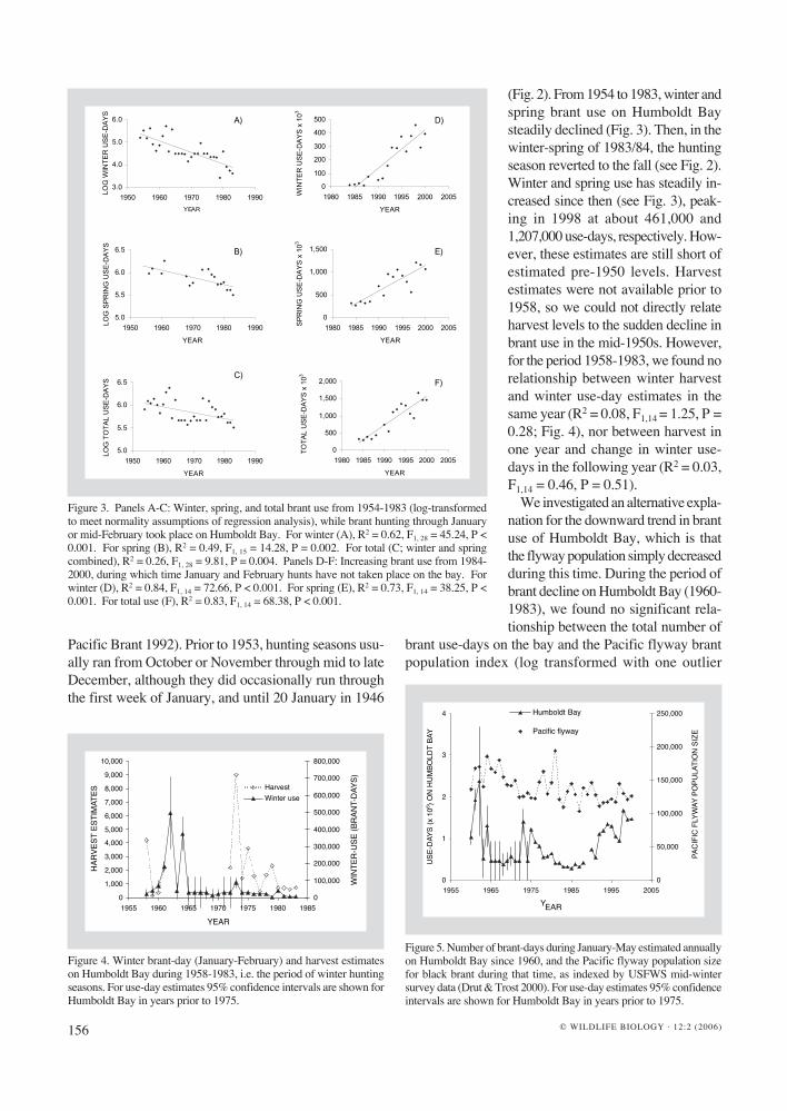
(Fig. 2). From 1954 to 1983, winter and spring brant use on Humboldt Bay steadily declined (Fig. 3). Then, in the winter-spring of 1983/84, the hunting season reverted to the fall (see Fig. 2). Winter and spring use has steadily in-creased since then (see Fig. 3), peak-ing in 1998 at about 461,000 and 1,207,000 use-days, respectively. How-ever, these estimates are still short of estimated pre-1950 levels. Harvest estimates were not available prior to 1958, so we could not directly relate harvest levels to the sudden decline in brant use in the mid-1950s. However, for the period 1958-1983, we found no relationship between winter harvest and winter use-day estimates in the same year (R2 = 0.08, F1,14 = 1.25, P = 0.28; Fig. 4), nor between harvest in one year and change in winter use-days in the following year (R2 = 0.03, F1,14 = 0.46, P = 0.51).

We investigated an alternative expla-nation for the downward trend in brant use of Humboldt Bay, which is that the flyway population simply decreased during this time. During the period of brant decline on Humboldt Bay (1960-1983), we found no significant rela-tionship between the total number of

brant use-days on the bay and the Pacific flyway brant population index (log transformed with one outlier

3.0

4.0

5.0

6.0

1950 1960 1970 1980 1990

YEAR

LOG

WIN

TE

R U

SE

-DA

YS

5.0

5.5

6.0

6.5

1950 1960 1970 1980 1990

YEAR

LOG

SP

RIN

G U

SE

-DA

YS

5.0

5.5

6.0

6.5

1950 1960 1970 1980 1990

YEAR

LOG

TO

TA

L U

SE

-DA

YS

0

100

200

300

400

500

1980 1985 1990 1995 2000 2005

YEAR

WIN

TE

RU

SE

-DA

YS

x10

3

0

500

1,000

1,500

1980 1985 1990 1995 2000 2005

YEAR

SP

RIN

GU

SE

-DA

YS

x10

3

0

500

1,000

1,500

2,000

1980 1985 1990 1995 2000 2005

YEAR

TO

TA

L U

SE

-DA

YS

x 1

03

)D)A

)E)B

C)F)

Figure 3. Panels A-C: Winter, spring, and total brant use from 1954-1983 (log-transformed to meet normality assumptions of regression analysis), while brant hunting through January or mid-February took place on Humboldt Bay. For winter (A), R2 = 0.62, F1, 28 = 45.24, P < 0.001. For spring (B), R2 = 0.49, F1, 15 = 14.28, P = 0.002. For total (C; winter and spring combined), R2 = 0.26, F1, 28 = 9.81, P = 0.004. Panels D-F: Increasing brant use from 1984-2000, during which time January and February hunts have not taken place on the bay. For winter (D), R2 = 0.84, F1, 14 = 72.66, P < 0.001. For spring (E), R2 = 0.73, F1, 14 = 38.25, P < 0.001. For total use (F), R2 = 0.83, F1, 14 = 68.38, P < 0.001.

0

1,000

2,000

3,000

4,000

5,000

6,000

7,000

8,000

9,000

10,000

1955 1960 1965 1970 1975 1980 1985

YEAR

HARV

EST

ESTI

MAT

ES

0

100,000

200,000

300,000

400,000

500,000

600,000

700,000

800,000

WIN

TER-

USE

(BRA

NT-D

AYS)

HarvestWinter use

Figure 4. Winter brant-day (January-February) and harvest estimates on Humboldt Bay during 1958-1983, i.e. the period of winter hunting seasons. For use-day estimates 95% confidence intervals are shown for Humboldt Bay in years prior to 1975.

0

1

2

3

4

1955 1965 1975 1985 1995 2005

YEAR

0

50,000

100,000

150,000

200,000

250,000Humboldt Bay

Pacific flyway

USE

-DAY

S (x

106 )

ON

HU

MBO

LDT

BAY

PAC

IFIC

FLY

WAY

PO

PULA

TIO

N S

IZE

Figure 5. Number of brant-days during January-May estimated annually on Humboldt Bay since 1960, and the Pacific flyway population size for black brant during that time, as indexed by USFWS mid-winter survey data (Drut & Trost 2000). For use-day estimates 95% confidence intervals are shown for Humboldt Bay in years prior to 1975.

14368 WB2_2006-v3.indd 156 13/06/06 10:32:01

157© WILDLIFE BIOLOGY · 12:2 (2006)

removed; R2 = 0.002, F1,22 = 0.04, P = 0.85; Fig. 5). Similarly, no relationship existed between population size and number of brant use-days during the period of increasing brant use on Humboldt Bay, which occurred from 1984 to 2000 (R2 = 0.08, F1,14 = 1.29, P = 0.27). Unfortunately, flyway data are not complete prior to 1960, so we could not test whether the dramatic decrease in use of Humboldt Bay in the early 1950s was associat-ed with a flyway level decline.

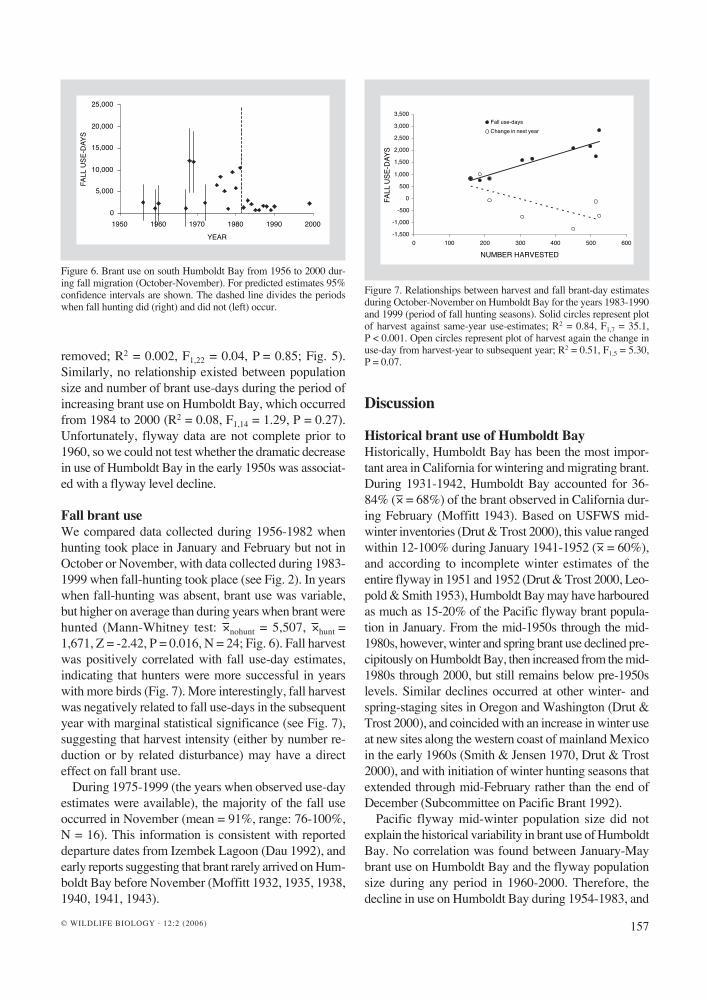
Fall brant useWe compared data collected during 1956-1982 when hunting took place in January and February but not in October or November, with data collected during 1983-1999 when fall-hunting took place (see Fig. 2). In years when fall-hunting was absent, brant use was variable, but higher on average than during years when brant were hunted (Mann-Whitney test: −×nohunt = 5,507, −×hunt = 1,671, Z = -2.42, P = 0.016, N = 24; Fig. 6). Fall harvest was positively correlated with fall use-day estimates, indicating that hunters were more successful in years with more birds (Fig. 7). More interestingly, fall harvest was negatively related to fall use-days in the subsequent year with marginal statistical significance (see Fig. 7), suggesting that harvest intensity (either by number re-duction or by related disturbance) may have a direct effect on fall brant use.

During 1975-1999 (the years when observed use-day estimates were available), the majority of the fall use occurred in November (mean = 91%, range: 76-100%, N = 16). This information is consistent with reported departure dates from Izembek Lagoon (Dau 1992), and early reports suggesting that brant rarely arrived on Hum-boldt Bay before November (Moffitt 1932, 1935, 1938, 1940, 1941, 1943).

Discussion

Historical brant use of Humboldt Bay Historically, Humboldt Bay has been the most impor-tant area in California for wintering and migrating brant. During 1931-1942, Humboldt Bay accounted for 36-84% (−× = 68%) of the brant observed in California dur-ing February (Moffitt 1943). Based on USFWS mid-winter inventories (Drut & Trost 2000), this value ranged within 12-100% during January 1941-1952 (−× = 60%), and according to incomplete winter estimates of the entire flyway in 1951 and 1952 (Drut & Trost 2000, Leo-pold & Smith 1953), Humboldt Bay may have harboured as much as 15-20% of the Pacific flyway brant popula-tion in January. From the mid-1950s through the mid-1980s, however, winter and spring brant use declined pre-cipitously on Humboldt Bay, then increased from the mid-1980s through 2000, but still remains below pre-1950s levels. Similar declines occurred at other winter- and spring-staging sites in Oregon and Washington (Drut & Trost 2000), and coincided with an increase in winter use at new sites along the western coast of mainland Mexico in the early 1960s (Smith & Jensen 1970, Drut & Trost 2000), and with initiation of winter hunting seasons that extended through mid-February rather than the end of December (Subcommittee on Pacific Brant 1992).

Pacific flyway mid-winter population size did not explain the historical variability in brant use of Humboldt Bay. No correlation was found between January-May brant use on Humboldt Bay and the flyway population size during any period in 1960-2000. Therefore, the decline in use on Humboldt Bay during 1954-1983, and

Figure 7. Relationships between harvest and fall brant-day estimates during October-November on Humboldt Bay for the years 1983-1990 and 1999 (period of fall hunting seasons). Solid circles represent plot of harvest against same-year use-estimates; R2 = 0.84, F1,7 = 35.1, P < 0.001. Open circles represent plot of harvest again the change in use-day from harvest-year to subsequent year; R2 = 0.51, F1,5 = 5.30, P = 0.07.

0

5,000

10,000

15,000

20,000

25,000

1950 1960 1970 1980 1990 2000

YEAR

FALL

USE

-DAY

S

Figure 6. Brant use on south Humboldt Bay from 1956 to 2000 dur-ing fall migration (October-November). For predicted estimates 95% confidence intervals are shown. The dashed line divides the periods when fall hunting did (right) and did not (left) occur.

-1,500

-1,000

-500

0

500

1,000

1,500

2,000

2,500

3,000

3,500

0 100 200 300 400 500 600

NUMBER HARVESTED

FALL

USE

-DAY

S

Fall use-daysChange in next year

14368 WB2_2006-v3.indd 157 13/06/06 10:32:02

158 © WILDLIFE BIOLOGY · 12:2 (2006)

the subsequent increase during 1984-2000, was not sim-ply tracking any such trend in the population as a whole.

Eelgrass condition has been suggested as a factor affect- ing brant use of Humboldt Bay based on few empirical data and anecdotal data (Einarsen 1965, Henry 1980). In the winters/springs of 1937/38, 1940/41, 1951/52, 1952/53, 1957/58 and 1997/98, substantial numbers of brant fed in salt marshes and pastures surrounding Humboldt Bay (Moffitt 1938, Moffitt 1941, Leopold & Smith 1953, Murrell 1962; HBNWR unpubl. report 1998). In all cases, this behaviour was attributed to poor feeding conditions on the bay, where eelgrass was ob-served covered with slimy or silty deposits, and/or infect-ed with Labyrinthula (implicated in the wasting disease of eelgrass on the Atlantic coast in the 1930s; Moffitt & Cottam 1941). Eelgrass in these years was greatly reduced in its extent and severely depleted by brant. However, in incidents prior to 1954, estimated brant use on Humboldt Bay remained high. Similarly, in the winter/spring of 1997/98, the greatest number of brant use-days in the last 25 years was recorded. Reduced food abundance on Humboldt Bay may thus affect brant feeding behaviour and habitat use, without reducing use of the overall area. The steady decline in brant use from the mid-1950s through the mid-1980s, if induced by poor eelgrass con-dition, would presumably have resulted from a long-term change in eelgrass habitat for which no evidence exists. In fact, several studies suggest that eelgrass was healthy and abundant from 1959 through 1962 (Murrell 1962, Keller 1963), in 1972 (Harding 1973), in 1975-1977 (Henry 1980), and in 1980-1981 (Bixler 1982). We therefore consider it unlikely that historical trends in brant use of Humboldt Bay could be explained by changes in quality or size of eelgrass habitat.

The most widely held view is that winter hunting dis-turbance from the 1950s to the 1980s reduced winter and spring brant use of Humboldt Bay and other sites in California, Oregon and Washington, and may have driv-en brant to new wintering sites in Mexico (Denson 1964, Smith & Jensen 1970, Henry 1980, Subcommittee on Pacific Brant 1992). During 1931-1953, when winter and spring brant use of Humboldt Bay was consistent-ly high, the hunting season began in October or Novem-ber, and typically ended by the end of December (see Fig. 2). This could have affected fall migrants, for which there are no data, but not spring migrants. During 1954-1983, the hunting season consistently ran through late January or mid-February (Subcommittee on Pacific Brant 1992), and declining winter and spring use of Hum-boldt Bay occurred during this time. Since 1983, hunt-ing seasons in California have been limited to fall months, during which time winter/spring use-days have

increased and fall use-days have decreased on Humboldt Bay. In Washington and Oregon also, hunting seasons have been more restrictive since 1983; during 1984-1986 there were no open seasons in these states, and since then seasons have been shorter and have ended earlier than before 1984 (Subcommittee on Pacific Brant 1992). Mid-winter survey data (Drut & Trost 2000) suggest that win-ter brant numbers in Washington have increased since the mid-1980s.

We cannot definitively conclude whether decreased brant use of U.S. sites was a cause or consequence of increased use in Mexico. However, it is not surprising that hunting might have had such an impact on brant use on Humboldt Bay and other U.S sites in general. Shifts in local and flyway-wide distributions due to hunting pressure have been documented in several other water-fowl populations (references in Fox & Madsen 1997, Bechet et al. 2003). Hunting activities apparently inter-rupt foraging time, increase energetic costs due to extra flying time, and displace birds to less profitable feeding areas (Fox & Madsen 1997, Madsen 1998) such that birds are unable to build adequate fat and nutrient reserves (Madsen 1995, Madsen & Fox 1995, Feret et al. 2003), a prerequisite to successful breeding in brant (Prop & Deerenberg 1991, Ebbinge & Spaans 1995) and other northern geese (Madsen 1995, 2001, Black et al. 1991, Prop & Black 1998). In addition, disturbances near tra-ditional grit sites and roosts may limit the birds’ ability to replenish gizzard grit thus reducing digestive efficien-cy. Wild geese are thought to adjust their foraging rou-tines on temporal and spatial scales to best achieve req-uisite fat and nutrient reserves (Owen & Black 1990, Prop et al. 2003). Geese that are unable to meet their dai-ly energetic needs are more likely to initiate movements to new areas (e.g. younger birds; Black 1998, Black et al. 1991), thus establishing new migratory traditions (Black et al. in press).

Detailed accounts of hunter disturbance (Murrell 1962, Henry 1980) describe south Humboldt Bay as being essentially unavailable to brant during a large portion of the hunting season. A narrow sand spit that separates South Bay from the ocean provides important roost and grit habitat to brant (Lee 2001), and is crossed by brant to enter the bay. Heavy hunting pressure along this spit prevents access to the bay and sand habitat, while inten-sive hunting from scull boats and offshore blinds pre-cludes use of sanctuary areas within eelgrass habitat. Such disturbance effects in January, and especially in February, could have consequences for brant use in March and April as well, if winter residents make up a significant fraction of the spring population. Lee (2001) found that spring-staging birds arriving to Humboldt

14368 WB2_2006-v3.indd 158 13/06/06 10:32:02

159© WILDLIFE BIOLOGY · 12:2 (2006)

Bay in late January through February stayed approxi-mately 30-50 days on average. Alternatively, social facil-itation may act such that brant on the bay in February attract later arrivals. This also seems plausible, given that later spring migrants are comprised of a greater frac-tion of juveniles (Henry 1980, Reed et al. 1998b, Lee 2001) who may need to learn the location of important staging areas from earlier arriving adults. Though unstud-ied in brant, related learning processes have been suggest-ed for juvenile Canada geese Branta canadensis (Williams & Kalmbach 1943, Surrendi 1970, Raveling 1976).

Hunting, in addition to its disturbance effects, might also reduce the number of use-days in an area simply by reducing local population numbers through hunting mor-tality. Adult brant show high fidelity to winter and spring-staging sites (Reed et al. 1998a), so high hunting mortality as seen in some years during 1958-1983 (see Fig. 3) could have long-term negative impacts for the number of use-days on Humboldt Bay. Harvest data do not exist for Humboldt Bay prior to 1958, so we could not rigorously evaluate whether extreme harvest mor-tality caused the sudden drop in brant use-days in the early 1950s. However, for years when harvest data were available, we found no relationship between winter har-vest intensity and winter use-day estimates, suggesting that overharvest may not have been the primary driver of winter or spring population trends on Humboldt Bay, at least since 1958. Furthermore, an 'overharvest hypoth-esis' does not predict increasing use of other areas in the flyway (i.e. Mexico). The coincident rise in use of Mexi-can sites in the 1960s therefore suggests that northbound migrants were not reduced by harvest on Humboldt Bay, but may have been displaced, so that for the past sever-al decades brant have spent most of January and February in Mexico rather than in the U.S. For southbound mi-grants, data do suggest that fall harvest intensity may have affected fall use-days in the subsequent year. Why might there be a relationship between harvest intensity and brant use-days in fall, but not winter and spring? One possibility is that while brant use-days are much higher in winter than in fall, harvest intensity has been similar in these two seasons. Fall-harvest numbers dur-ing 1983-2000 (Median = 304; 1st-3rd quartiles: 290-440) were of comparable magnitude to winter harvest estimates between 1958 and 1983 (Median = 1,490; 1st-3rd quartiles: 684-2,235), whereas fall brant use during 1984-2000 (Median = 1,638, 1st-3rd quartiles: 819-2,086) was roughly 20 times lower than estimated win-ter use during 1958-1983 (Median = 30,028, 1st-3rd quartiles: 21,064-38,722). Thus, we might expect a giv-en level of harvest to have a greater measurable effect on fall brant use-days.

Human population and industrialization surrounding Humboldt Bay has increased, as has related sources of non-hunting human disturbance to brant. These changes have been quantified by Henry (1980) and Schmidt (1999), who identified the activities of clam fishermen, recreational and commercial boaters, oyster culture, low-flying aircraft, and vehicle traffic (especially off-road vehicles) on the east shore of South Bay (South Spit) as the most significant contributors. In addition, a tempo-rary camping settlement on South Spit was described as a major deterrent to brant use at roost and grit sites dur-ing the first half of the 1990s (HBNWR, unpubl. reports 1991-1995). We agree with previous authors that these factors are likely to have played a role in reducing win-ter and spring brant use-days following the early 1950s, and suggest that persistent human disturbance could pre-vent brant use-days from returning to historical levels. However, these non-hunting disturbances are probably not solely responsible for the overall trends in brant use-days observed over the past 70 years. Based on our his-torical estimates, Humboldt Bay suffered a steep drop in brant use in 1953 or 1954, which persisted and declined further through the mid-1980s. This decline definitely coincided with a change in timing of winter hunting sea-sons, whereas there is no indication that other sources of disturbance also occurred in a punctuated and then persistent manner. Furthermore, the number of winter and spring brant use-days have increased since the ces-sation of winter hunting in the mid-1980s, despite prob-able increases in non-hunting human disturbance.

While January and February brant use has increased in response to fall hunting seasons, December use (while hunting is occurring) has not similarly responded, hav-ing remained consistently low on Humboldt Bay since at least the 1960s. Occasional high counts in December during the 1930s and 1950s, along with large January counts during the 1940s, suggest that larger numbers of brant arrived earlier, at least in some years, than they do today. Increased winter use along the mainland coast of Mexico has presumably resulted in fewer brant moving up into California before January, so while winter use on Humboldt Bay has increased in the absence of hunt-ing disturbance, the arrival of brant is still somewhat delayed each year.

Since 1956, fall use has been low and irregular on Humboldt Bay, although higher on average in years without fall hunting. During fall migration, most brant fly non-stop from Alaska to Mexico (Dau 1992), and early reports suggest that relatively few brant stopped at Hum- boldt Bay in fall (Moffitt 1932). The variability of fall use in non-hunting years can probably be explained by the fact that Humboldt Bay is not a major fall-staging

14368 WB2_2006-v3.indd 159 13/06/06 10:32:02

160 © WILDLIFE BIOLOGY · 12:2 (2006)

ground, so numbers are more likely to depend on annu-al variation in weather patterns and the number of birds unable to make the otherwise non-stop migration (Dau 1992).

Management implicationsCollection of long-term data on single species is valu-able for management, but may be costly and difficult to maintain. Conversely, studies of shorter duration often preclude analysis of historical trends in population size, distribution and habitat condition and use. We suggest that accurate predictions of brant use-days (Ra

2 > 0.90) at Humboldt Bay can be derived from single mid-month-ly counts from January through April, thus lowering the costs and facilitating the establishment of a long-term monitoring program, though such a protocol should be revalidated and calibrated periodically via thorough esti-mation of seasonal brant use-days.

Using this method, we extrapolated historical brant use of Humboldt Bay, which enabled us to identify long-term trends and investigate factors thought to affect them. We suggest that 30 years of hunting disturbance during early spring migration resulted directly in declin-ing brant use during 1953-1983. Other forms of distur-bance and habitat conditions probably contributed rela-tively little to this decline. This conclusion has been assumed by wildlife managers, who have responded by maintaining a fall hunt in California since 1984. The results of our study empirically affirm the appropriate-ness of the current policy; relieving hunting pressure has increased brant use of Humboldt Bay. However, this poses a challenge to managers of how to provide hunt-ing opportunities without driving brant away from important migration areas.

Acknowledgements - we thank K. Forrest, R.J. Guadagno and M. Drut for providing us with, and interpreting, histori-cal brant survey reports. We are grateful to D. Yparraguirre who helped us see the many complexities involved in water-fowl management. We also thank Dan, along with T. Fox, D. Ward, S.E. Sheaffer, and two anonymous reviewers for their helpful comments on earlier versions of this manuscript.

References

Ankney, C.D. 1984: Nutrient reserve dynamics of breeding and molting brant. - Auk 101: 361-370.

Barnhart, R.A., Boyd, M.J. & Pequegnat, J.E. 1992: The Ecol-ogy of Humboldt Bay, California: An Estuarine Profile. - U.S. Fish and Wildlife Service Biological Report 1, 121 pp.

Bechet, A., Giroux, J.F., Gauthier, G., Nichols, J.D. & Hines, J.E. 2003: Spring hunting changes the regional movements

of migrating greater snow geese. - Journal of Applied Ecol-ogy 40: 553-564.

Bixler, R.P. 1982: Primary productivity of eelgrass Zostera marina L.: comparative rates and methods. - Master’s the-sis, Humboldt State University, Arcata, California, USA, 38 pp.

Black, J.M. 1998: Movement of barnacle geese between col-onies in Svalbard and the colonisation process. - Norsk Polar-institutt Skrifter 200: 115-127.

Black, J.M., Deerenberg, C. & Owen, M. 1991: Foraging be-haviour and site selection of barnacle geese in a traditional and newly colonized spring staging area. - Ardea 79: 349-358.

Black, J.M., Prop, J. & Larsson, K. in press: Wild goose dilem-mas: population consequences of individual decisions in bar-nacle geese. - Branta Press, Groningen, The Netherlands.

Dau, C.P. 1992: The fall migration of Pacific flyway brent Branta bernicla in relation to climatic conditions. - Wildfowl 43: 80-95.

Denson, E.P. 1961: Waterfowl populations and a comparison of hunting methods on South Humboldt Bay, California, 1959-1960. - Master’s thesis, Humboldt State University, Arcata, California, USA, 124 pp.

Denson, E.P. 1964: Comparison of waterfowl hunting tech-niques at Humboldt Bay, California. - Journal of Wildlife Management 28: 103-119.

Denson, E.P. & Murrell, S.L. 1962: Black brant populations of Humboldt Bay, California. - Journal of Wildlife Man-agement 26: 257-262.

Drut, M.S. & Trost, R.E. 2000: 2000 Pacific Flyway Data Book: Waterfowl harvests and status, hunter participation and success, and certain hunting regulations in the Pacific fly-way and United States. - U.S. Fish and Wildlife Service, 145 pp.

Ebbinge, B.S. & Spaans, B. 1995: The importance of body reserves accumulated in spring staging areas in the temper-ate zone for breeding in dark-bellied brent geese Branta b. bernicla in the high Arctic. - Journal of Avian Biology 26: 105-113.

Einarsen, A.S. 1965: Black brant: sea goose of the Pacific coast. - University of Washington Press, 142 pp.

Feret, M., Gauthier, G., Bechet, A., Giroux, J.F. & Hobson, K.A. 2003: Effect of a spring hunt on nutrient storage by greater snow geese in southern Quebec. - Journal of Wildlife Management 67: 796-807.

Fox, A.D. & Madsen, J. 1997: Behavioural and distributional effects of hunting disturbance on waterbirds in Europe: implications for refuge design. - Journal of Applied Ecology 34: 1-13.

Harding, L.W. 1973: Primary production in Humboldt Bay. - Master’s thesis, Humboldt State University, Arcata, Cali-fornia, USA, 55 pp.

Harding, L.W. & Butler, J.H. 1979: The standing stock of pro-duction of eelgrass, Zostera marina, in Humboldt Bay, Cali-fornia. - California Fish and Game 65: 151-158.

Henry, W.G. 1980: Populations and behavior of black brant at Humboldt Bay, California. - Master’s thesis, Humboldt State University, Arcata, California, USA, 111 pp.

14368 WB2_2006-v3.indd 160 13/06/06 10:32:03

161© WILDLIFE BIOLOGY · 12:2 (2006)

Keller, M. 1963: The growth and distribution of eelgrass Zostera marina L. in Humboldt Bay, California. - PhD thesis, Humboldt State University, Arcata, California, USA, 53 pp.

Lee, D.E. 2001: Immigration, emigration, stopover duration, and volume of black brant migrating through Humboldt Bay, California. - Master’s thesis. Humboldt State University, Arcata, California, USA, 44 pp.

Leopold, A.S. & Smith, R.H. 1953: Numbers and winter dis-tribution of Pacific black brant in North America. - California Fish and Game 39: 95-101.

Madsen, J. 1995: Impacts of disturbance on migratory water-fowl. - Ibis 137: S67-S74.

Madsen, J. 1998: Experimental refuges for migratory water-fowl in Danish wetlands. II. Tests of hunting disturbance effects. - Journal of Applied Ecology 35: 398-417.

Madsen, J. 2001: Spring migration strategies in pink-footed geese Anser brachyrhynchus and consequences for spring fattening and fecundity. - Ardea 89: 43-55.

Madsen, J. & Fox, A.D. 1995: Impact of hunting disturbance on waterbirds - a review. - Wildlife Biology 1: 193-207.

Moffitt, J. 1931: First annual black brant census in California. - California Fish and Game 17: 396-401.

Moffitt, J. 1932: Second annual black brant census in California. - California Fish and Game 18: 298-310.

Moffitt, J. 1933: Third annual black brant census in California. - California Fish and Game 19: 255-263.

Moffitt, J. 1934: Fourth annual black brant census in California. - California Fish and Game 20: 355-364.

Moffitt, J. 1935: Fifth annual black brant census in California. - California Fish and Game 21: 343-350.

Moffitt, J. 1936: Sixth annual black brant census in California. - California Fish and Game 22: 295-300.

Moffitt, J. 1937: Seventh annual black brant census in California. - California Fish and Game 23: 290-295.

Moffitt, J. 1938: Eighth annual black brant census in California. - California Fish and Game 24: 341-346.

Moffitt, J. 1939: Ninth annual black brant census in California. - California Fish and Game 25: 336-342.

Moffitt, J. 1940: Tenth annual black brant census in California. - California Fish and Game 26: 381-389.

Moffitt, J. 1941: Eleventh annual black brant census in California. - California Fish and Game 27: 216-223.

Moffitt, J. 1943: Twelfth annual black brant census in California. - California Fish and Game 29: 19-28.

Moffitt, J. & Cottam, C. 1941: Eelgrass depletion on the Pacific coast and its effect upon black brant. - U.S. Fish and Wildlife Service, Wildlife Leaflet No. 204, 26 pp.

Moore, J.E., Colwell, M.A., Mathis, R.L. & Black, J.M. 2004: Spring staging of black brant throughout the Pacific Flyway in relation to eelgrass abundance and site isolation, with spe-cial consideration of Humboldt Bay, California. - Biological Conservation 115: 475-486.

Murrell, S.L. 1962: A study of crippling loss, kill and aging techniques of black brant (Branta nigricans), at Humboldt

Bay, California. - Master’s thesis, Humboldt State University, Arcata, California, USA, 56 pp.

Owen, M. & Black, J.M. 1990: Waterfowl Ecology. - Glasgow, Blackie Publishers, 194 pp.

Proctor, C.M., Garcia, J.C., Galvin, D.V., Lewis, G.B., Loehr, L.C. & Massa, A.M. 1980: An ecological characterization of the Pacific Northwest coastal region. - United States Fish and Wildlife Service, FWS/OBS-79/11-15, 1746 pp.

Prop, J. & Black, J.M. 1998: Food intake, body reserves and reproductive success of barnacle geese Branta leucopsis staging in different habitats. - Norsk Polarinsitutts Skrifter 200: 175-193.

Prop, J., Black, J.M. & Shimmings, P. 2003: Travel schedules to the high arctic: barnacle geese trade-off the timing of migration with accumulation of fat deposits. - Oikos 103: 403-414.

Prop, J. & Deerenberg, C. 1991: Spring staging in brent geese Branta bernicla: feeding constraints and the impact of diet on the accumulation of body reserves. - Oecologia 87: 19-28.

Raveling, D.G. 1976: Migration reversal: a regular phenome-non of Canada geese. - Science 193: 153-154.

Reed, A., Cooch, E.G., Goudie, R.I. & Cooke, F. 1998a: Site fidelity of black brant wintering and spring staging in the Strait of Georgia, British Columbia. - Condor 100: 426-437.

Reed, A., Ward, D.H., Derksen, D.V. & Sedinger, J.S. 1998b: Brant Branta bernicla. - In: Poole, A. & Gill, F. (Eds.); The Birds of North America. The American Ornithologists’ Union, No. 337, 32 pp.

Schmidt, P.E. 1999: Population counts, time budgets, and dis-turbance factors of black brant (Branta bernicla nigricans) at Humboldt Bay, California. - Master’s thesis, Humboldt State University, Arcata, California, USA, 48 pp.

Smith, R.H. & Jensen, G.H. 1970: Black brant on the main-land coast of Mexico. - Transactions of the North American Wildlife and Natural Resources Conference 35: 227-241.

Subcommittee on Pacific Brant 1992: Pacific Flyway manage-ment plan for Pacific brant. - Pacific Flyway Study Com-mittee (c/o USFWS, MBMO), Portland, Oregon, USA, Unpublished Report, 75 pp.

Surrendi, D.C. 1970: The mortality, behavior, and homing of transplanted juvenile Canada geese. - Journal of Wildlife Management 34: 719-733.

Terra-Mar Humboldt Bay Orthophoto (USGS Map Ref. Ca0006-av3020) 1997: Vol. NCGIC 98.8-51. - Terra-mar Resource Information Services, Inc., Mountain View, Cali-fornia. Distributed by North Coast Geographic Information Cooperative, Arcata, CA.

Waddell, J.E. 1964: The effect of oyster culture on eelgrass Zostera marina L. growth. - Master’s thesis, Humboldt State University, Arcata, California, USA, 48 pp.

Williams, C.S. & Kalmbach, E.R. 1943: Migration and fate of transported juvenile waterfowl. - Journal of Wildlife Manage-ment 7: 163-169.

14368 WB2_2006-v3.indd 161 13/06/06 10:32:03

162 © WILDLIFE BIOLOGY · 12:2 (2006)

Appendix I. Regression equations used to estimate winter, spring or total brant use-days during 1931-1974 (all F1-5, 18-23 > 27, P < 0.001). Equations were derived from 1975-2000 data, but were based on count dates from pre-1975 years. For example, in 1949 one count was con-ducted during the second week of January. Therefore 1975-2000 data were used to determine the relationship between winter use-days and a count conducted in this week. The regression relationship was then used to predict winter use-days in 1949 from that year’s count.

Prediction variable Years Explanatory variablesa Regression equation Adjusted R2

Winter use-days 1964-67, 71-72, 74 1st week of January Y = 30029 + 128 (Jan) 0.891949 2nd week of January Y = 24263 + 100 (Jan) 0.801947 3rd week of January Y = 25386 + 58 (Jan) 0.941944 4th week of January Y = 19851 + 53 (Jan) 0.951943, 45, 48, 50-53, 58, 63 January peak Y = 17491 + 53 (Jan) 0.971931 1st week of February Y = 12794 + 43 (Feb) 0.981933-34, 36-39 2nd week of February Y = 4783 + 35 (Feb) 0.941935 Model 1: 1st week of February

Model 2: 2nd week of February (averaged)Model 1: Y = 12794 + 43 (Feb)Model 2: Y = 4783 + 35 (Feb)

0.96

1955 3rd week of February Y = 6505 + 27 (Feb) 0.871954 4th week of February Y = 4909 + 21 (Feb) 0.731956 February peak Y = 1418 + 21 (Feb) 0.781968-69 1st week of January, 1st week of February Y = 13492 + 24 (Jan) + 36 (Feb) 0.981962, 70 1st week of January, February peak Y = 7489 + 89 (Jan) + 9 (Feb) 0.951932 3rd week of January, 2nd week of February Y = 10213 + 42 (Jan) + 14 (Feb) 0.971940-42 January peak, 2nd week of February Y = 7848 + 43 (Jan) + 10 (Feb) 0.991957, 59-61, 73 January and February peaks Y = 4965 + 41 (Jan) + 6 (Feb) 0.99

Spring use-days 1933, 37-38, 56, 58 1-15 March Y = 47217 + 47 (Mar) 0.801970 1-15 March, April peak Y = -67043 + 40 (Mar) + 15 (Apr) 0.851973 February peak, March peak Y = 95571 + 20 (Feb) + 24 (Mar) 0.821968-69 March peak, April peak Y = 6867 + 24 (Mar) + 14 (Apr) 0.691939 2nd week of February, 16-31 March,

16-30 AprilY = -6251 + 28 (Feb) + 23 (Mar) + 24 (Apr) 0.89

1957, 60, 61 February peak, 16-31 March, 16-30 April Y = 3555 + 19 (Feb) +22 (Mar) + 22 (Apr) 0.94Total use-days 1964-67, 71-72, 74 1st week of January Y = 459878 + 312 (Jan) 0.66

1949 2nd week of January Y = 451577 + 198 (Jan) 0.521947 3rd week of January Y = 461033 + 139 (Jan) 0.661944 4th week of January Y = 478181 + 121 (Jan) 0.611943, 45, 48, 50-53, 63 January peak Y = 474309 + 120 (Jan) 0.621931 1st week of February Y = 460186 + 100 (Feb) 0.651932, 34, 40-42 2nd week of February Y = 438531 + 78 (Feb) 0.561935 Model 1: 1st week of February

Model 2: 2nd week February (averaged)Model 1: Y = 460186 + 100 (Feb)Model 2: Y = 438531 + 78 (Feb)

0.60

1955 3rd week of February Y = 442475 + 65 (Feb) 0.561954 4th week of February Y = 400270 + 54 (Feb) 0.611959 February peak Y = 405249 + 54 (Feb) 0.641962 1 January, February peak Y = 367556 + 153 (Jan) + 36 (Feb) 0.751958 January peak, 1-15 March Y = 63720 + 57 (Jan) + 47 (Mar) 0.881970 1st week of January, 1-15 March, April peak Y = -47048 + 157 (Jan) + 36 (Mar) + 17 (Apr) 0.911957, 60, 61 January peak, February peak, 16-31 March,

16-30 AprilY = 12881 + 39 (Jan) + 26 (Feb) + 21 (Mar) + 22 (Apr)

0.97

1968, 69 1 February, March peak, April peak Y = -1337 + 77 (Feb) + 17 (Mar) + 17 (Apr) 0.911939 2 February, 16-31 March, 16-30 April Y = 2649 + 63 (Feb) + 23 (Mar) + 23 (Apr) 0.921933, 37-38 2 February, 1-15 March Y = 63590 + 39 (Feb) + 45 (Mar) 0.871956 February peak, 1-15 March Y = 44817 + 25 (Feb) + 46 (Mar) 0.871973 February peak, March peak Y = 83882 + 40 (Feb) + 25 (Mar) 0.87

a indicates that count was either a monthly peak value, or that it was conducted within the particular 1 or 2-week period specified. If multiple counts were conducted within this time period, the largest one was used, both for deriving the regression equations (1975-2000 data) and for entering pre-1975 into these equations to estimate historical values.

14368 WB2_2006-v3.indd 162 13/06/06 10:32:03