© 1991 IEEE. Reprinted with permission, from IEEE Journal of Robotics and Automation, Vol. 7, No. 4, 1991, pp. 535-539.

HISTOGRAMIC IN-MOTION MAPPINGFOR MOBILE ROBOT OBSTACLE AVOIDANCE

byJ. Borenstein , Member IEEE and Y. Koren , Senior Member IEEE

Department of Mechanical Engineering and Applied MechanicsThe University of Michigan, Ann Arbor, MI 48109

ABSTRACT

This paper introduces histogramic in-motion mapping (HIMM), a new method for real-timemap building with a mobile robot in motion. HIMM represents data in a two-dimensional array,called a histogram grid, that is updated through rapid in-motion sampling of onboard rangesensors. Rapid in-motion sampling results in a map representation that is well-suited to modelinginaccurate and noisy range-sensor data, such as that produced by ultrasonic sensors, and requiresminimal computational overhead. Fast map-building allows the robot to immediately use themapped information in real-time obstacle-avoidance algorithms. The benefits of this integratedapproach are twofold: (1) quick, accurate mapping; and (2) safe navigation of the robot toward agiven target.

HIMM has been implemented and tested on a mobile robot. Its dual functionality wasdemonstrated through numerous tests in which maps of unknown obstacle courses were created,while the robot simultaneously performed real-time obstacle avoidance maneuvers at speeds of upto 0.78 m/sec.

Page 2

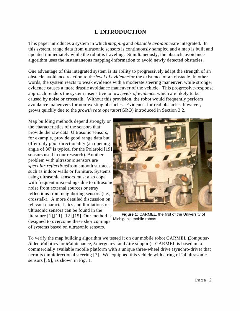
Figure 1: CARMEL, the first of the University ofMichigan's mobile robots.

1. INTRODUCTION

This paper introduces a system in which mapping and obstacle avoidance are integrated. Inthis system, range data from ultrasonic sensors is continuously sampled and a map is built andupdated immediately while the robot is traveling. Simultaneously, the obstacle avoidancealgorithm uses the instantaneous mapping-information to avoid newly detected obstacles.

One advantage of this integrated system is its ability to progressively adapt the strength of anobstacle avoidance reaction to the level of evidence for the existence of an obstacle. In otherwords, the system reacts to weak evidence with a moderate steering maneuver, while strongerevidence causes a more drastic avoidance maneuver of the vehicle. This progressive-responseapproach renders the system insensitive to low levels of evidence, which are likely to becaused by noise or crosstalk. Without this provision, the robot would frequently performavoidance maneuvers for non-existing obstacles. Evidence for real obstacles, however,grows quickly due to the growth rate operator (GRO) introduced in Section 3.2. Map building methods depend strongly onthe characteristics of the sensors thatprovide the raw data. Ultrasonic sensors,for example, provide good range data butoffer only poor directionality (an openingangle of 30 is typical for the Polaroid [19]o

sensors used in our research). Anotherproblem with ultrasonic sensors arespecular reflections from smooth surfaces,such as indoor walls or furniture. Systemsusing ultrasonic sensors must also copewith frequent misreadings due to ultrasonicnoise from external sources or strayreflections from neighboring sensors (i.e.,crosstalk). A more detailed discussion onrelevant characteristics and limitations ofultrasonic sensors can be found in theliterature [1],[11],[12],[15]. Our method isdesigned to overcome these shortcomingsof systems based on ultrasonic sensors. To verify the map building algorithm we tested it on our mobile robot CARMEL (Computer-Aided Robotics for Maintenance, Emergency, and Life support). CARMEL is based on acommercially available mobile platform with a unique three-wheel drive (synchro-drive) thatpermits omnidirectional steering [7]. We equipped this vehicle with a ring of 24 ultrasonicsensors [19], as shown in Fig. 1.

Page 3

This paper focuses on the map building aspect of our system, rather than on the obstacleavoidance algorithms. A comprehensive discussion of our two obstacle avoidance methods,the Virtual Force Field (VFF) and the Vector Field Histogram (VFH) method, is given in[2],[3], and in [4],[5], respectively. Section 2 evaluates related work in map building, andSection 3 explains our real-time map building method in detail.

2. MAP BUILDING WITH ULTRASONIC SENSORS

In order to create a map from ultrasonic range measurements, the environment must first bescanned. To do so, many mobile robots are equipped with 24 sensors that are mounted on ahorizontal ring around the robot [2], [6], [8], [14], [17]. Ring scanning does not requirerotating parts and motors, and a full 360 panorama can be acquired rapidly. However, allo

sensors cannot be fired at once, since this would cause significant crosstalk. Special scanningsequences can be designed that reduce crosstalk, but increase the overall time needed toobtain a full panorama (i.e., all 24 sensors). Typical scan times range from 100 to 500 ms, fora full panorama.

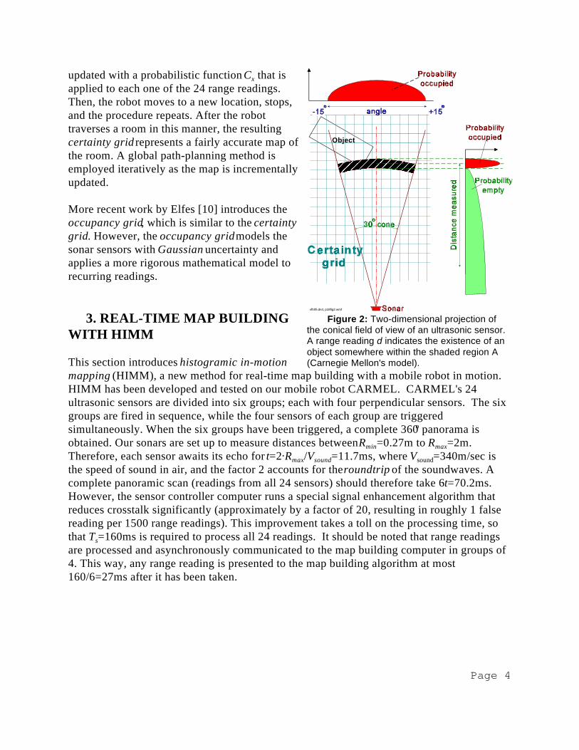
A pioneering method for probabilistic representation of obstacles in a grid-type world modelhas been developed at Carnegie-Mellon University (CMU) [9],[16],[17]. The resulting worldmodel, called a certainty grid, is especially suited to the unified representation of data fromdifferent sensors such as ultrasonic, vision, and proximity sensors [17], as well as the accom-modation of inaccurate sensor data such as range measurements from ultrasonic sensors. With the certainty grid world model, the robot's work area is represented by a two-dimensional array of square elements denoted as cells. Each cell contains a certainty value(CV) that indicates the measure of confidence that an obstacle exists within the cell area. CVsare updated by a heuristic probability function that takes into account the characteristics of agiven sensor. For example, ultrasonic sensors have a conical field of view. A typicalultrasonic sensor [19] returns a radial measure of the distance to the nearest object within thecone, yet does not specify the angular location of the object. Thus, a distance measurement dresults from an object located anywhere within the area A (see Fig. 2). However, an objectlocated near the acoustic axis (the center of the cone) is more likely to produce an echo thanan object further away from the acoustic axis [1]. Consequently, with the CMU method, CVsare assigned to all cells in A, but higher values are assigned to cells closer to the acoustic axis,according to a heuristic probability function.

Additional information can be derived from a range reading concerning the sector between Sand A (see Fig. 2). If an echo is received from an object at distance d, then this sector must befree of objects. In [9] and [16] this is expressed by applying a probability function withnegative values to the cells in the empty area.

In CMU's original certainty grid method [9],[16],[17], the mobile robot remains stationarywhile taking a panoramic scan with its ring of 24 ultrasonic sensors. The certainty grid is

vfh05.ds4, p18fig2.wmf

Object

Page 4

Figure 2: Two-dimensional projection ofthe conical field of view of an ultrasonic sensor.A range reading d indicates the existence of anobject somewhere within the shaded region A(Carnegie Mellon's model).

updated with a probabilistic function C that isx

applied to each one of the 24 range readings.Then, the robot moves to a new location, stops,and the procedure repeats. After the robottraverses a room in this manner, the resultingcertainty grid represents a fairly accurate map ofthe room. A global path-planning method isemployed iteratively as the map is incrementallyupdated.

More recent work by Elfes [10] introduces theoccupancy grid, which is similar to the certaintygrid. However, the occupancy grid models thesonar sensors with Gaussian uncertainty andapplies a more rigorous mathematical model torecurring readings.

3. REAL-TIME MAP BUILDINGWITH HIMM

This section introduces histogramic in-motionmapping (HIMM), a new method for real-time map building with a mobile robot in motion. HIMM has been developed and tested on our mobile robot CARMEL. CARMEL's 24ultrasonic sensors are divided into six groups; each with four perpendicular sensors. The sixgroups are fired in sequence, while the four sensors of each group are triggeredsimultaneously. When the six groups have been triggered, a complete 360 panorama iso

obtained. Our sonars are set up to measure distances between R =0.27m to R =2m.min max

Therefore, each sensor awaits its echo for t=2 R /V =11.7ms, where V =340m/sec ismax sound sound

the speed of sound in air, and the factor 2 accounts for the roundtrip of the soundwaves. Acomplete panoramic scan (readings from all 24 sensors) should therefore take 6t=70.2ms.However, the sensor controller computer runs a special signal enhancement algorithm thatreduces crosstalk significantly (approximately by a factor of 20, resulting in roughly 1 falsereading per 1500 range readings). This improvement takes a toll on the processing time, sothat T =160ms is required to process all 24 readings. It should be noted that range readingss

are processed and asynchronously communicated to the map building computer in groups of4. This way, any range reading is presented to the map building algorithm at most160/6=27ms after it has been taken.

We use this term in the literal sense of "likelihood."1

Page 5

3.1 The Histogram Grid

HIMM uses a two-dimensional Cartesian histogram grid for obstacle representation. Thisrepresentation has been derived from the certainty grid concept described in Section 2. Likethe certainty grid, each cell in the histogram grid holds a certainty value (CV) that representsthe confidence of the algorithm in the existence of an obstacle at that location. The histogramgrid differs from the certainty grid in the way it is built and updated. CMU's method projectsa probability profile onto all those cells affected by a range reading (i.e., all cells in the area Aof Fig. 2). This procedure is computationally intensive and might impose a time-penalty onreal-time execution by an onboard computer. Our method, on the other hand, increments onlyone cell in the histogram grid for each range reading. For ultrasonic sensors, the incrementedcell is the one that corresponds to the measured distance d (see Fig. 3a) and lies on theacoustic axis of the sensor. While this approach may seem to be an oversimplification, aprobability distribution is actually obtained by continuously and rapidly sampling each1

sensor while the vehicle is moving. Thus, the same cell and its neighboring cells arerepeatedly incremented, as shown in Fig. 3b. This results in a histogramic probabilitydistribution, in which high certainty values are obtained in cells close to the actual location ofthe obstacle. Note that the HIMM method is less accurate when the robot is stationary. Acomparative evaluation of the accuracy of our method is given in [20].

HIMM makes use of the "empty sector" between S and A (see Fig. 4), as does CMU'scertainty grid method [9],[16]. However, instead of computing and projecting a negativeprobability function for all cells in the sector, we take advantage of our fast samplingapproach and decrement only those cells that are located on the line connecting center cell Cc

and origin cell C (i.e., the acoustic axis, in Fig. 4).o

A final note concerns the actual implementation of HIMM: Whenever a cell is incremented,the increment (denoted I ) is actually 3 (not 1, as may be expected) and the maximum CV of a+

cell is limited to CV =15. Decrements (denoted I), however, take place in steps of -1 andmax-

the minimum value is CV =0. Note that CV and CV have been chosen arbitrarily. Imin max min+

was determined experimentally (in relation to CV ), by observing that too large a valuemax

would make the robot react to single, possibly false readings, while a smaller value would notbuild up CVs in time for an avoidance maneuver. I was determined experimentally and in-

relation to I . I must be smaller than I because only one cell is incremented for each reading,+ - +

whereas multiple cells might be decremented for one reading (i.e., all cells between C and C ,c o

in Fig. 4). Note that it is exceedingly difficult to formulate a mathematically rigorousrelationship between those parameters. The reason is the large number of unknowns thataffect a general formulation. For example, an object may be "seen" at a certain instance byone or more sensors simultaneously. Whether or not an echo is received depends on therelative angles, the surface structure, the reflectiveness of the object, and the distance to the

Object Object

currentreading

vfh10.ds4, p18fig3.wmf

Page 6

Figure 3: a. Only one cell is incremented for each range reading. With ultrasonic

sensors, this is the cell that lies on the acoustic axis and corresponds tothe measured distance d.

b. A histogramic probability distribution is obtained by continuous and rapidsampling of the sensors while the vehicle is moving.

object.

HIMM is part of areal-time obstacleavoidance system; itnot only producesmaps but alsoprovidesinstantaneousenvironmentalinformation for useby the integratedobstacle avoidancealgorithm. Tounderstand how thisfunction issupported, it isnecessary tomention somecharacteristics ofour vector fieldhistogram (VFH)method for real-timeobstacle avoidance. A detailed discussion of the VFH method is given in [4] and [5].

To increase the signal-to-noise ratio, the obstacle avoidance response of the VFH algorithm isproportional to the square of a CV. We will call this the Squared Certainty Value (SCV). Forexample, if five readings have incremented a particular cell (i,j), then CV =5 3=15, andi,j

SCV =(15) =225. We introduce the SCV to express our confidence that recurring rangei,j2

readings represent actual obstacles (as opposed to single readings, which may be caused bynoise or crosstalk). Furthermore, the VFH obstacle avoidance response is stronger when acluster of SCVs is encountered, whereas single, unclustered cells provoke only a mildresponse. For this reason, we will define the term Obstacle Cluster Strength (OCS) as the sumof all SCVs in a certain cluster (i.e., a grouping of neighboring cells with CV>0).

3.2 Fast Mapping for Real-time Obstacle Avoidance

HIMM, as explained so far, serves two functions: a) it produces high CVs for cells thatcorrespond to obstacles, and b) it keeps low CVs for cells that were incremented due to mis-readings (e.g., noise or crosstalk) or moving objects. For slow-moving vehicles, this systemworks very well; yet when a vehicle is traveling at relatively high speeds (e.g., V>0.5m/sec),matters are more complicated. The following example explains one of these problems. Note

+3

-1

-1-1-1-1-1-1-1-1-1-1-1-1-1

C0p18f4bw.drw, p18f4bw.pcx, 3/11/91

For simplicity, we assume here that only one sensor can "see" the object, as is often the case with2

thin vertical poles or pipes.

Page 7

Figure 4: Information on the emptysector between S and A is used todecrement all cells along line C ) C .0 c

that the numerical values in this example correspond to actual specifications of our mobilerobot CARMEL. Other systems will have different values, but the principle will be the same.

Suppose CARMEL approaches a thin vertical pole whiletraveling at its maximum speed V =0.78 m/sec. Tomax

avoid a collision at this speed, CARMEL must begin anavoidance maneuver at a distance of approximatelyD=100 cm from the obstacle, as shown in Fig. 5. Theobstacle is initially detected by the robot at R =200 cm.max

Thus, the HIMM algorithm has at most t =(R -c max

D)/V =1.28 sec to produce an OCS strong enough tomax

cause an avoidance maneuver. Since each sensor is firedonce every T =160 msec, the robot can sample at mostp

n =t /T =8 readings from the same sensor . Note that n isc c p c2

the critical number of readings needed to provoke anavoidance maneuver.

A map building algorithm with simultaneous real-timeobstacle avoidance must thus build a significant OCSquickly and from few readings, while maintaining a highcontrast with erroneous readings (i.e., high signal-to-noise ratio). This task is further complicated by in-motion sampling, as the following example shows:

When a stationary ultrasonic sensor is repeatedlysampled, it will usually increment the same cell for anobstacle, even if that cell does not accurately correspondto the obstacle. Assuming the robot was able to take n readings, the CV of that cell willc

reach the maximum value, CV=15, with an OCS = 15 = 225. The resulting cluster comprises2

of one cell only. Actually, only 5 readings were needed to reach CV=15; the remaining 3readings are "lost" because of the limit CV . In-motion sampling, on the other hand, willmax

usually cause the same n sonar readings to be scattered over several neighboring cells, evenc

when the obstacle is a thin pole. This might result in a cluster such as the one shown inFig. 6a. In this example, eight range readings were taken and projected onto the histogramgrid in the following order: two readings - cell a; two readings - cell b; one reading each -cells c,d,e, and f. This cluster yields OCS = 6 +6 +3 +3 +3 +3 = 108, which is less than thescat

2 2 2 2 2 2

OCS that would result from the same number of readings by a stationary sensor (225). Ingeneral, if n readings (with n < CV /I ) are scattered equally over neighboring cells, theymax

+

will result in OCS =n(I ) which is smaller then OCS =(nI ) , which results when all nscat single c+ 2 + 2

Page 8

Figure 5: With a maximum range of R =200cm and a minimal avoidancemax

distance D=100 cm, CARMEL has 1.28 sec to produce an obstacle clusterstrength (OCS) strong enough to cause an avoidance maneuver.

Figure 6: a. In-motion sampling causes sonar readings of an object to bescattered over several cells, resulting in a low OCS.

b. 3×3 mask for growth rate operator (GRO).c. With the GRO, OCSs are built up fast and from

few readings.

readings are projected intoone cell. As was mentionedin Section 3.2, it isimperative for fast, real-timeobstacle avoidance that ahigh OCS is built quickly, inorder to cause a strongavoidance maneuver in time.

To compensate for theadverse scattering effectcaused by in-motionsampling, we introduce amethod to significantlyincrease the growth rate ofan OCS (when readings arescattered in neighboringcells). This method uses agrowth rate operator (GRO)to increment a cell (i,j) fasterwhen the immediate neighbors of the cell hold high CVs. This function is implemented inreal-time by convolving CV with the 3×3 mask given in Fig. 6b, and adding the usuali,j

increment I =3, yielding+

p,q=1CV' = CV + I + (w CV ) (1)i,j i,j p,q i+p,j+q

+

p,q=-1

Page 9

whereCV previous certainty value of cell (i,j),i,j

CV' updated certainty value of cell (i,j),i,j

I constant increment (I =3),+ +

w weighing factor.

with w =0.5 for p=±1 and q=±1, and w =1 for p=q=0p,q p,q

Unlike mask operators in computer vision algorithms, where the operator is applied to everypixel after an image has been sampled, the GRO (by means of Eq. 1) is applied to each rangereading as it is projected onto the histogram grid.

The following numeric example demonstrates the function of the GRO. Using Eq. (1) to re-construct the histogram grid in the previous example of Fig. 6a (assuming cells are read andupdated in the same order), we obtain the cluster shown in Fig 6c. The individual steps of thiscomputation are listed in Table I, and the OCS of this cluster is OCS =6 +12 +GRO

2 2

12 +15 +15 +15 =999.2 2 2 2

Table I: Example computation of an OCS using the growth rate operator (GRO) in Fig. 6b.

Reading Cell CV'))))))))))))))))))))))))))))))))))))))))))))))))))))))1 a = a + I = 0 + 3 = (3)+

2 a = a + I = 3 + 3 = 6+

3 b = b + I + ½(a) = 0 + 3 + 3 = (6)+

4 b = b + I + ½(a) = 6 + 3 + 3 = 12+

5 c = c + I + ½(a+b) = 0 + 3 + 9 = 12+

6 d = d + I + ½(a+b+c) = 0 + 3 + 15 = 15+ *

7 e = e + I + ½(b+d) = 0 + 3 + 13.5 = 15+ *

8 f = f + I + ½(e+f) = 0 + 3 + 15 = 15+ *

))))))))))))))))))))))))))))))))))))))))))))))))))))) Note that CVs are limited to CV = 15; *

max( ) denote temporary values.

It should be clear that the GRO has little or no effect on erroneous readings. Erroneousreadings (due to noise or crosstalk) appear randomly and usually effect single, unclusteredcells, and are filtered out by the algorithm discussed above.

The only disadvantage of the GRO is the following: Without the GRO, high CVs areusually obtained at the actual location of an object, while lower CVs (due to the inaccuraciesof the sensors) are scattered around the borders of the object. With the GRO, however, low-certainty areas adjacent to high-certainty areas build up to high CVs, resulting in a tendencyto represent obstacles larger then they really are. This distortion, however, is not verysignificant; furthermore, we can fine-tune the trade-off between more accurate maps and

Page 10

faster OCS build-up by adjusting the weighing factor w. Reducing w reduces the effect of theGRO, and completely cancels the effect with w=0. It is also possible to set w adaptively to theinstantaneous speed of the mobile robot.

4. Experimental Results

The map building algorithms were tested on CARMEL. This platform has a maximumtravel speed of V =0.78m/sec and a maximum steering rate of =120deg/sec; it weighsmax

about 125kg. A Z-80 on-board computer serves as the low-level controller of the vehicle. Two computers were added to the platform: a 20Mhz, 80386-based AT-compatible that runsthe integrated obstacle-avoidance/map-building algorithm, and a PC-compatible single-boardcomputer to control the sensors.

Fig. 7 shows the result of an experimental run. Three layers of information are depicted inthis figure:

a. The robot's path, starting at S and ending at T, is plotted as the curved line. This pathresulted from an actual run of our mobile robot, with real-time obstacle avoidance bythe VFH method. CARMEL's average speed in this run was 0.54m/sec and themaximum speed was 0.78m/sec.

b. Obstacles and walls are shown as solid lines. Objects labeled "partitions" are two-inch-thick styrofoam sheets with smooth surfaces. The object labeled "pole" is a 3/4inch cardboard pipe, and the object labeled "box" is a cardboard box. In general,poles do not cause specular reflections and are thus easy to detect from all directions.The pole in Fig. 7, however, is very slender and produces only a very weak echo,much weaker than a flat wall or a pole of larger diameter.

c. The histogram grid is also reproduced in Fig. 7. Empty cells are not shown, whilefilled cells are represented by small black rectangles (blobs). Each cell represents areal-world square of size 10cm×10cm. While the certainty values in our system mayrange from 0 to 15, the screen-dump of Fig. 7a can only show classes of low,medium, and high CVs, distinguished by different blob sizes. Note that the left sideof partition a is outside of the range limit of the ultrasonic sensors, and so are most ofthe walls.

In order to convert the histogram grid into a permanent map, we define an arbitrarythreshold, e.g., CV =12. Any CV<CV is rejected (i.e., set to zero). This conversionthres thres

results in the final grid-type map shown in Fig. 7b for the histogram grid in Fig. 7a.

During a typical run through a densely cluttered obstacle course, CARMEL's speed mayvary considerably: from 0.8 m/sec to sometimes as low as 0.04 m/sec [2]. In a given timeinterval, more range readings are taken in a certain area when the robot travels at low speeds,

Page 11

Figure 7: a. A real-time run with CARMEL, showing the robot's path, the actuallocation of the unexpected obstacles, and the resulting histogram grid.

b. The histogram grid after thresholding with CV =12.thres

adding undue weight to these readings. However, this undesirable effect is constrained by theupper bound of CV =15, which limits the CV for any given cell. On the other hand, due tomax

the GRO, cells reach CV quickly and with only a few readings even when the robot ismax

traveling at high speeds.

5. CONCLUSIONS

HIMM, a new method for combined real-time map building and obstacle avoidance hasbeen introduced and tested. In this method, inaccurate ultrasonic sensor data is statisticallymodeled in a two-dimensional histogram grid. A histogramic probability representation isobtained through rapid, continuous sampling of the sensors during motion. With HIMM, anyrange reading is immediately represented in the map and has immediate influence on theconcurrent obstacle avoidance algorithm.

Further optimization, by means of the growth rate operator (GRO) allows the HIMMmethod to build high-contrast representations based on only a few range readings. Thisfeature is essential for the robot to react quickly to unexpected obstacles, even when travelingat high speeds.

Page 12

AcknowledgementsThis work was sponsored by the Department of Energy Grant DE-FG02-

86NE37969

6. REFERENCES

1. Borenstein, J. and Koren, Y., "Obstacle Avoidance With Ultrasonic Sensors." IEEEJournal of Robotics and Automation, Vol. RA-4, No. 2, 1988, pp. 213-218.

2. Borenstein, J. and Koren, Y., "Real-time Obstacle Avoidance for Fast MobileRobots." IEEE Transactions on Systems, Man, and Cybernetics, Vol. 19, No. 5,Sept/Oct 1989, pp. 1179-1187.

3. Borenstein, J. and Koren, Y., "Tele-autonomous Guidance for Mobile Robots." IEEETransactions on Systems, Man, and Cybernetics, special issue on unmanned systemsand vehicles, December 1990, pp. 1437-1443.

4. Borenstein, J. and Koren, Y., "Real-time Obstacle Avoidance for Fast Mobile Robotsin Cluttered Environments." 1990 IEEE International Conference on Robotics andAutomation, Cincinnati, Ohio, May 13-18, 1990, pp. 572-577.

5. Borenstein, J. and Koren, Y., "The Vector Field Histogram ) Fast ObstacleAvoidance for Mobile Robots." IEEE Journal of Robotics and Automation, Vol. 7,No. 3., June 1991, pp. 278-288..

6. Crowley, J. L., "World Modeling and Position Estimation for a Mobile Robot UsingUltrasonic Ranging." Proceedings of the 1989 IEEE International Conference onRobotics and Automation, Scottsdale, Arizona, May 14-19, 1989, pp. 674-680.

7. Cybermation, "K2A Mobile Platform." Commercial Offer, 5457 JAE Valley Road,Roanoke, Virginia 24014, 1989.

8. Denning Mobile Robotics, Inc., "Securing the Future." Commercial Offer, 21Cummings Park, Woburn, MA 01801, 1985.

9. Elfes, A., "Sonar-based Real-World Mapping and Navigation." IEEE Journal ofRobotics and Automation, Vol. RA-3, No 3, 1987, pp. 249-265.

10. Elfes, A, "Using Occupancy Grids for Mobile Robot Perception and Navigation."Computer Magazine, June 1989, pp. 46-57.

Page 13

11. Everett, H. R., "A Multielement Ultrasonic Ranging Array." Robotics Age, July 1985,pp. 16-20.

12. Flynn, A. M., "Combining Sonar and Infrared Sensors for Mobile RobotNavigation." The International Journal of Robotics Research, Vol. 7, No. 6,December 1988, pp. 5-14.

13. Kadonoff, M. B., et al., "Arbitration of Multiple Control Strategies for MobileRobots." Proceedings of the SPIE, Mobile Robots (1986), Vol. 727, 1986, pp. 90-98.

14. Korba, L. W., Liscano, R., and Durie, N., "An Intelligent Mobile Platform for HealthCare Applications." Proceedings of the ICAART 88 conference, Montreal, Canada,1988, pp. 462-463.

15. Kuc, R. and Barshan, B., "Navigating Vehicles Through an UnstructuredEnvironment With Sonar." Proceedings of the 1989 IEEE International Conferenceon Robotics and Automation. Scottsdale, Arizona, May 14-19, 1989, pp. 1422-1426.

16. Moravec, H. P. and Elfes, A., "High Resolution Maps from Wide Angle Sonar."Proceedings of the IEEE Conference on Robotics and Automation, Washington,D.C., 1985, pp. 116-121.

17. Moravec, H. P., "Sensor Fusion in Certainty Grids for Mobile Robots." AI Magazine,Summer 1988, pp. 61-74.

18. Pin, F. G. et al., "Autonomous Mobile Robot Research Using the Hermies-III Robot."IROS International Conference on Intelligent Robot and Systems, Tsukuba, Japan,Sept. 1989.

19. POLAROID Corporation, Ultrasonic Components Group, 119 Windsor Street,Cambridge, Massachusetts 02139, 1989.

20. Raschke, U. and Borenstein, J., "A Measure of Performance for Grid-type Map-building Techniques," to be presented at the 1990 IEEE International Conference onRobotics and Automation, Cincinnati, Ohio, May 13-18, 1990, pp. 1828-1832.

List of Footnotes

We use this term in the literal sense of "likelihood."1

For simplicity, we assume here that only one sensor can "see" the object, as is often the case with2

thin vertical poles or pipes.