Hille-Yosida Theorem

and some Applications

Apratim De

Supervisor: Professor Gheorghe Moros,anu

Submitted to:

Department of Mathematics and its Applications

Central European University

Budapest, Hungary

CE

UeT

DC

olle

ctio

n

Acknowledgements

First and foremost, I would like to express my special appreciation and

sincere gratitude to my supervisor, Professor Gheorghe Moros,anu for his

constant support and encouragement, and his invaluable advice and guid-

ance. He has been a tremendous mentor and I am honored to have had

the opportunity of working with a mathematician of his stature.

I would like to extend my special thanks to Prof. Karoly Boroczky

and Prof. Pal Hegedus for their guidance, and unending support and

patience. I would also like to thank Ms. Elvira Kadvany and Ms. Melinda

Balazs for being the best coordinators of any department I have been a

part of, always ready to extend their helping hand whenever I needed, and

all my teachers and colleagues whom I came to know during my wonderful

time at the Mathematics Department at CEU.

I am especially thankful to my parents for everything they’ve done

for me and last but not the least, I would like to thank my best friends,

Ella and Alfredo whose unwavering support and belief in me have helped

me through my most trying times. This work is dedicated to them.

CE

UeT

DC

olle

ctio

n

Contents

Introduction 1

1 Preliminaries 2

1.1 Maximal monotone operators and their

properties . . . . . . . . . . . . . . . . . . . . . . . . . . . . . . . . . 2

1.2 Lp spaces . . . . . . . . . . . . . . . . . . . . . . . . . . . . . . . . . 4

1.3 Sobolev spaces . . . . . . . . . . . . . . . . . . . . . . . . . . . . . . 5

1.4 Open sets of class Cm . . . . . . . . . . . . . . . . . . . . . . . . . . 8

1.5 Sobolev embedding theorems . . . . . . . . . . . . . . . . . . . . . . . 9

1.6 Green’s identity for Sobolev Spaces . . . . . . . . . . . . . . . . . . . 11

1.7 Variational formulation of the Dirichlet

boundary value problem for the Laplacian . . . . . . . . . . . . . . . 13

2 Hille-Yosida Theorem 16

2.1 Existence and uniqueness of solution to the evolution problem dudt

+

Au = 0 on [0,+∞) with initial data u(0) = u0 . . . . . . . . . . . . . 16

2.2 Regularity of the solutions . . . . . . . . . . . . . . . . . . . . . . . . 33

2.3 The case of self-adjoint operators . . . . . . . . . . . . . . . . . . . . 39

3 Applications of Hille-Yosida Theorem 51

3.1 Heat Equation . . . . . . . . . . . . . . . . . . . . . . . . . . . . . . . 51

3.2 Wave Equation . . . . . . . . . . . . . . . . . . . . . . . . . . . . . . 63

3.3 Linearized equations of coupled sound and heat flow . . . . . . . . . . 71

Bibliography 86

i

CE

UeT

DC

olle

ctio

n

Introduction

The main focus of this work is going to be the Hille-Yosida theorem, which, as we

will see, is a very powerful tool in solving evolution partial differential equations. The

material is organized as follows. Chapter 1 presents the background material needed

for the treatment in the subsequent chapters. In Chapter 2, we present the Hille-

Yosida Theorem and related results and offer detailed proofs. Finally, in Chapter 3,

we investigate applications of the Hille-Yosida theorem to some real word phenomena.

We prove existence, uniqueness and regularity of solutions of the Heat equation, the

Wave equation, and the linearized equations of coupled sound and heat flow. For the

proofs of most of the results established in Chapter 1, relevant references are cited

wherever needed. The subsequent chapters are self-contained.

1

CE

UeT

DC

olle

ctio

n

Chapter 1

Preliminaries

This chapter is going to be our toolbox of important concepts and results that we

will use time and again throughout the course of this Thesis.

1.1 Maximal monotone operators and their

properties

Here we will only consider single-valued operators but to account for the general case

of multi-valued operators, a good way to define an operator A on a set X is to simply

consider A as a subset of the Cartesian product X × X. Then we can define the

domain of A as

D(A) = u ∈ X|∃v such that [u, v] ∈ A.

We use the notation [u, v] to denote an element of the Cartesian product so as not

to confuse with a scalar product which we will denote by (·, ·). Note that for a single

valued operator A, D(A) = u ∈ X|∃v ∈ X such that Au = v. We also define the

range of A as

R(A) =⋃

u∈D(A)

Au.

For the case of single valued operators Au can be considered as the singleton set

Au.Henceforth, we will only focus on operators defined on a real Hilbert space, H.

Definition. An operator A on a Hilbert space H is called monotone if

(y2 − y1, x2 − x1) ≥ 0 ∀ [x1, y1], [x2, y2] ∈ A.

2

CE

UeT

DC

olle

ctio

n

Note that for a single valued linear operator A, it is monontone if (Au, u) ≥ 0 ∀u ∈D(A).

Definition. An operator A on a Hilbert space H is called maximal monotone if:

(i) A is monotone.

(ii) A has no proper monotone extension. That is, for any monotone operator

A′ ⊂ H ×H if A ⊆ A′, then A = A′.

Theorem 1.1.1 (G. Minty). Suppose A : D(A) ⊂ H → H is a monotone operator.

Then A is maximal monotone iff R(A+ I) = H.

This is a very important result used in identifying maximal monotone operators.

In fact, sometimes, this is taken as the definition of maximal operators.

Proposition 1.1.2. Let A be a linear maximal monotone operator. Then we have:

(i) D(A) is dense in H;

(ii) A is a closed operator;

(iii) (I + λA) is a bijection from D(A) onto H for every λ > 0. Moreover,

(I + λA)−1 is a bounded operator and∥∥(I + λA)−1

∥∥L(H)≤ 1.

Remark 1.1.1 We see from Theorem 1.1.1 that the following are equivalent:

(i) A is a maximal monotone operator.

(ii) λA+ I is surjective for all λ > 0.

(iii) λA+ I is surjective for some λ > 0.

That is, A is maximal monotone iff λA is maximal monotone for some λ > 0; iff λA

is maximal montone for all λ > 0.

It also holds that A+λI is surjective for some some λ > 0 if and only if A is maximal

monotone.

Definition. Let A be a maximal monotone operator. For every λ > 0, we define the

following operators:

Jλ = (I + λA)−1, Aλ =1

λ(I − Jλ).

3

CE

UeT

DC

olle

ctio

n

Jλ is called the resolvent, and Aλ, the Yosida approximation of A. Note that D(Jλ) =

D(Aλ) = H, R(Jλ) = D(A) and if A is linear, then ‖Jλ‖L(H) ≤ 1.

The resolvent and Yosida approximation (named after Kosaku Yosida) have many

useful properties that make them an invaluable tool in proving the Hille-Yosida The-

orem (Theorem 2.1.3). We list some of their properties as follows.

Proposition 1.1.3. Let A be a linear maximal monotone operator. Then we have

the following:

(i) Aλv = A(Jλv) ∀ v ∈ H, ∀λ > 0,

(ii) Aλv = Jλ(Av) ∀ v ∈ D(A), ∀λ > 0,

(iii) |Aλv| ≤ |Av| ∀ v ∈ D(A),∀ λ > 0,

(iv) limλ→0 Jλv = v ∀ v ∈ H,

(v) limλ→0Aλv = Av ∀ v ∈ D(A),

(vi) (Aλv, v) ≥ 0 ∀v ∈ H,∀ λ > 0,

(vii) |Aλv| ≤ 1λ|v| ∀v ∈ H,∀ λ > 0.

For further reference regarding the material of this section, see [2], [1].

1.2 Lp spaces

Let us denote R = (−∞,∞); N = 0, 1, 2, · · · . Let X be a real real Banach space

with the norm ‖·‖X and Ω ⊂ RN for some integer N ≥ 1 be a Lebesgue measurable

set.

Definition. Let 1 ≤ p <∞. Then we define Lp(Ω;X) as the space of all equivalence

classes of (strongly) measurable functions f : Ω → X such that x 7→ ‖f(x)‖pX is

Lebesgue integrable and the equivalence relation is equality a.e on Ω.

In general when we write, u ∈ Lp(Ω;X), we mean u is a representative of the

equivalence class of functions that agree with u a.e on Ω. Lp(Ω;X) is a real Banach

space witht he norm

‖u‖Lp(Ω;X) =

(∫Ω

‖u(x)‖pX) 1

p

.

4

CE

UeT

DC

olle

ctio

n

For p = ∞, we define L∞(Ω;X) as the space of equivalence classes of measurable

functions f : Ω → X such that x 7→ ‖f(x)‖X is essentially bounded. L∞(Ω;X) is a

real Banach space with the norm

‖u‖L∞(Ω;X) = ess supx∈Ω

‖u(x)‖X .

When X = R, we use the notation Lp(Ω). If Ω = (a, b) ⊂ R, we write Lp(a, b;X).

For more background material regarding this section , see [2].

1.3 Sobolev spaces

In this section, we will define Sobolev spaces. First, we establish some notations.

Here, we assume Ω is a non-empty open subset of RN . We denote by Ck(Ω) the space

of functions that are continuous on Ω and have continuous partial derivatives up to

order k. We also define:

C∞(Ω) = φ ∈ C(Ω)|φ has continuous partial derivatives of any order ,

C∞c (Ω) = φ ∈ C∞(Ω)|supp φ is compact in Ω ,

where supp φ = x ∈ Ω | φ(x) 6= 0. Let 1 ≤ p ≤ ∞.

Definition. The Sobolev space W 1,p(Ω) is defined as

W 1,p(Ω) =

u ∈ Lp(Ω)

∣∣∣∣∃g1, g2, ..., gN ∈ Lp(Ω) such that∫Ωu ∂ϕ∂xi

= −∫

Ωgiϕ, ∀ϕ ∈ C∞c (Ω), ∀i = 1, · · · , N

For u ∈ W 1,p(Ω), we define ∂u

∂xi= gi. This definition makes sense since gi is unique

a.e (this follows from the fact that∫

Ωfϕ = 0 ∀ϕ ∈ C∞c (Ω) ⇒ f = 0 a.e on Ω). Here

∂u∂xi

denotes the weak derivative.

For p = 2, we write, H1(Ω) = W 1,2(Ω). The space W 1,p(Ω) equipped with the norm

‖u‖W 1,p =

(‖u‖pLp +

N∑i=1

∥∥∥∥ ∂u∂xi∥∥∥∥pLp

) 1p

for 1 ≤ p <∞

and

‖u‖W 1,∞ = ‖u‖L∞ +N∑i=1

∥∥∥∥ ∂u∂xi∥∥∥∥L∞

for p =∞

5

CE

UeT

DC

olle

ctio

n

is a real Banach space. The space H1(Ω) is equipped with the scalar product

(u, v)H1 = (u, v)L2 +N∑i=1

(∂u

∂xi,∂v

∂xi

)L2

=

∫Ω

uv +N∑i=1

∫Ω

∂u

∂xi

∂v

∂xi

=

∫Ω

uv +

∫Ω

N∑i=1

∂u

∂xi

∂v

∂xi

=

∫Ω

uv +

∫Ω

∇u · ∇v.

H1(Ω) is a real Hilbert space with this scalar product and the associated norm is

‖u‖H1 =

(∫Ω

u2 +

∫Ω

|∇u|2) 1

2

.

Remark 1.3.1. If u ∈ C1(Ω) ∩ Lp(Ω), and if ∂u∂xi∈ Lp(Ω) for all i = 1, · · · , N (here

∂u∂xi

denotes the partial derivative in the usual sense), then u ∈ W 1,p(Ω) and the usual

partial derivatives coincide with their Sobolev counterparts. So our notations are

consistent.

Definition. For integers m ≥ 2 and 1 ≤ p ≤ ∞, we define the Sobolev space

Wm,p(Ω) inductively as follows:

Wm,p(Ω) =

u ∈ Wm−1,p(Ω)

∣∣∣∣ ∂u∂xi ∈ Wm−1,p(Ω) ,∀i = 1, · · · , N.

Equivalently, we can define:

Wm,p(Ω) =

u ∈ Lp(Ω)

∣∣∣∣∀α, with |α| ≤ m,∃gα ∈ Lp(Ω) such that∫ΩuDαϕ = (−1)|α|

∫Ωgαϕ, ∀ϕ ∈ C∞c (Ω).

,

where we use the standard multi-index notation α = (α1, α2, · · · , αN) with αi ≥ 0 ,

an integer and |α| =∑N

i=1 αi and

Dαϕ =∂|α|ϕ

∂xα11 · · · ∂x

αNN

.

We denote Dαu = gα, and as before, this is well-defined. The space Wm,p(Ω) equipped

with the norm

‖u‖Wm,p =

∑|α|≤m

‖Dαu‖pLp

1p

for 1 ≤ p <∞

6

CE

UeT

DC

olle

ctio

n

and

‖u‖Wm,p =∑|α|≤m

‖Dαu‖L∞ for p =∞

is a real Banach space. We write Hm(Ω) = Wm,2(Ω). The space Hm(Ω) equipped

with the scalar product

(u, v)Hm =∑|α|≤m

(Dαu,Dαv)L2

is a real Hilbert space.

Definition. Let 1 ≤ p ≤ ∞. The Sobolev space Wm.p0 (Ω) is defined as the closure

of C∞c (Ω) in Wm,p(Ω). More precisely, u ∈ Wm,p0 (Ω) iff ∃ a sequence of functions ,

un ∈ C∞c (Ω) such that ‖u− un‖Wm,p → 0.

As before, we write Hm0 (Ω) = Wm,2

0 (Ω).

Remark 1.3.2 Consider Ω = RN+ . Then Γ = ∂Ω = RN−1 × 0. In this case it can

be shown that the map u 7→ u|Γ defined from C∞c (RN) into Lp(Γ) extends by density

to a bounded linear operator from W 1,p(Ω) into Lp(Γ). The operator is defined to be

the trace of u on Γ and it is also denoted by u|Γ.

Now if Ω is a regular open set in RN , e.g., if Ω is of class C1 with Γ = ∂Ω bounded,

then it is possible to define the trace of a function u ∈ W 1,p(Ω) on Γ = ∂Ω. In this

case, u|Γ ∈ Lp(Γ) (for the surface measure dσ).

One important result regarding the trace is as follow: the kernel of the trace

operator is W 1,p0 (Ω), that is,

W 1,p0 (Ω) =

u ∈ W 1,p(Ω) | u|Γ = 0

.

For further reference, see [11], [2].

7

CE

UeT

DC

olle

ctio

n

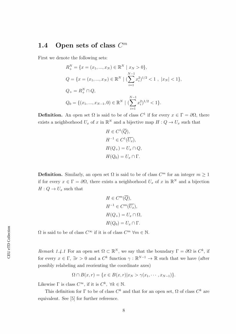
1.4 Open sets of class Cm

First we denote the following sets:

RN+ = x = (x1, ..., xN) ∈ RN | xN > 0,

Q = x = (x1, ..., xN) ∈ RN | (N−1∑i=1

x2i )

1/2 < 1 , |xN | < 1,

Q+ = RN+ ∩Q,

Q0 = (x1, ..., xN−1, 0) ∈ RN | (N−1∑i=1

x2i )

1/2 < 1.

Definition. An open set Ω is said to be of class C1 if for every x ∈ Γ = ∂Ω, there

exists a neighborhood Ux of x in RN and a bijective map H : Q→ Ux such that

H ∈ C1(Q),

H−1 ∈ C1(Ux),

H(Q+) = Ux ∩Q,

H(Q0) = Ux ∩ Γ.

Definition. Similarly, an open set Ω is said to be of class Cm for an integer m ≥ 1

if for every x ∈ Γ = ∂Ω, there exists a neighborhood Ux of x in RN and a bijection

H : Q→ Ux such that

H ∈ Cm(Q),

H−1 ∈ Cm(Ux),

H(Q+) = Ux ∩ Ω,

H(Q0) = Ux ∩ Γ.

Ω is said to be of class C∞ if it is of class Cm ∀m ∈ N.

Remark 1.4.1 For an open set Ω ⊂ RN , we say that the boundary Γ = ∂Ω is Ck, if

for every x ∈ Γ, ∃r > 0 and a Ck function γ : RN−1 → R such that we have (after

possibly relabeling and reorienting the coordinate axes)

Ω ∩B(x, r) = x ∈ B(x, r)|xN > γ(x1, · · · , xN−1).

Likewise Γ is class C∞, if it is Ck, ∀k ∈ N.

This definition for Γ to be of class Ck and that for an open set, Ω of class Ck are

equivalent. See [5] for further reference.

8

CE

UeT

DC

olle

ctio

n

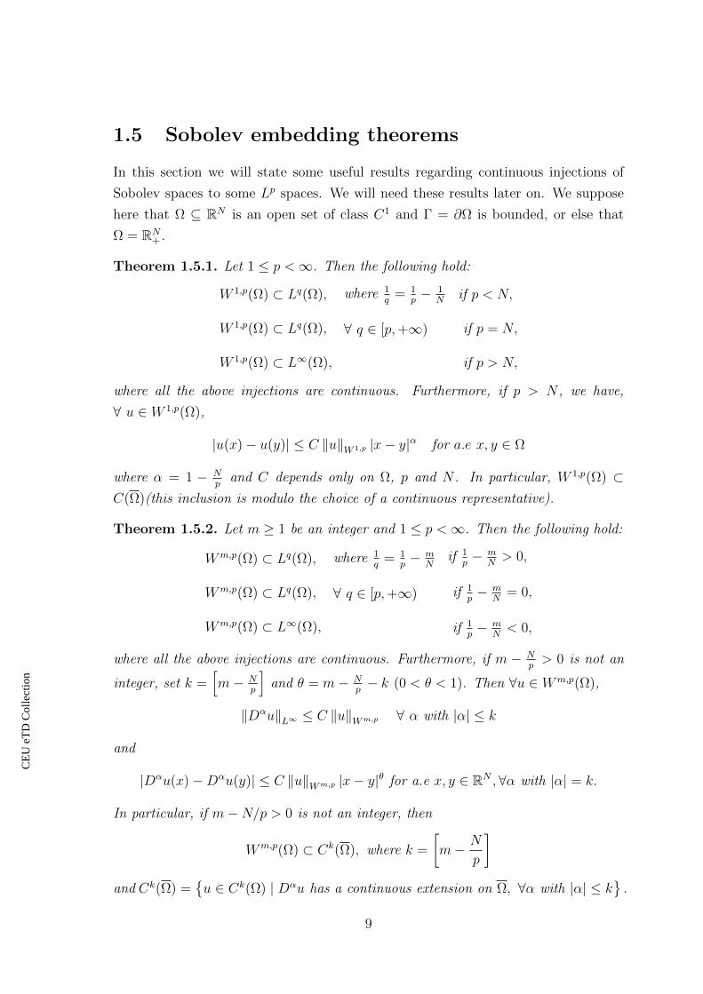
1.5 Sobolev embedding theorems

In this section we will state some useful results regarding continuous injections of

Sobolev spaces to some Lp spaces. We will need these results later on. We suppose

here that Ω ⊆ RN is an open set of class C1 and Γ = ∂Ω is bounded, or else that

Ω = RN+ .

Theorem 1.5.1. Let 1 ≤ p <∞. Then the following hold:

W 1,p(Ω) ⊂ Lq(Ω),

W 1,p(Ω) ⊂ Lq(Ω),

W 1,p(Ω) ⊂ L∞(Ω),

where 1q

= 1p− 1

N

∀ q ∈ [p,+∞)

if p < N,

if p = N,

if p > N,

where all the above injections are continuous. Furthermore, if p > N , we have,

∀ u ∈ W 1,p(Ω),

|u(x)− u(y)| ≤ C ‖u‖W 1,p |x− y|α for a.e x, y ∈ Ω

where α = 1 − Np

and C depends only on Ω, p and N . In particular, W 1,p(Ω) ⊂C(Ω)(this inclusion is modulo the choice of a continuous representative).

Theorem 1.5.2. Let m ≥ 1 be an integer and 1 ≤ p <∞. Then the following hold:

Wm,p(Ω) ⊂ Lq(Ω),

Wm,p(Ω) ⊂ Lq(Ω),

Wm,p(Ω) ⊂ L∞(Ω),

where 1q

= 1p− m

N

∀ q ∈ [p,+∞)

if 1p− m

N> 0,

if 1p− m

N= 0,

if 1p− m

N< 0,

where all the above injections are continuous. Furthermore, if m − Np> 0 is not an

integer, set k =[m− N

p

]and θ = m− N

p− k (0 < θ < 1). Then ∀u ∈ Wm,p(Ω),

‖Dαu‖L∞ ≤ C ‖u‖Wm,p ∀ α with |α| ≤ k

and

|Dαu(x)−Dαu(y)| ≤ C ‖u‖Wm,p |x− y|θ for a.e x, y ∈ RN ,∀α with |α| = k.

In particular, if m−N/p > 0 is not an integer, then

Wm,p(Ω) ⊂ Ck(Ω), where k =

[m− N

p

]and Ck(Ω) =

u ∈ Ck(Ω) | Dαu has a continuous extension on Ω, ∀α with |α| ≤ k

.

9

CE

UeT

DC

olle

ctio

n

Proofs. (c.f. [2] , [5])

Corollary 1.5.3. Given any k ∈ N, there exists an integer m > k such that

Wm,2(Ω) ⊂ Ck(Ω) and this inclusion is a continuous injection.

Proof. if Ω ⊂ RN , where N is odd, then for sufficiently large m > N2

, we have that

m−N2> 0 is not an integer and it follows from Theorem 1.5.2 that Wm,2(Ω) ⊂ Ck(Ω).

Now if N is even, choose m1 = N2

, an integer. Then it follows from Theorem 1.5.2,

that

Wm1,2(Ω) ⊂ Lq(Ω) is a continuous injection (1.5.1)

for some irrational q > 2. Now let’s choose an integer m2 =[k + N

q

]+ 1. Then

m2 − Nq> 0 is not an integer and by Theorem 1.5.2 with k =

[m2 − N

q

],

Wm2,q(Ω) ⊂ Ck(Ω) (1.5.2)

is a continuous injection. Now, since Wm1,2(Ω) ⊂ Lq(Ω),

u ∈ Wm1+1,2(Ω) =

u ∈ Wm1,2(Ω) | ∂u

∂xi∈ Wm1,2(Ω), ∀ i = 1, ..., N

⇒ u ∈ Lq(Ω),

∂u

∂xi∈ Lq(Ω), ∀ i = 1, ..., N.

Therefore, u ∈ W 1,q(Ω), that is, Wm1+1,2 ⊂ W 1,q(Ω). Also note that Wm1+1,2(Ω) ⊂Wm1,2(Ω) ⊂ Lq(Ω), where each injection is continuous. Now,

‖u‖2Wm1+1,2 = ‖u‖2

Wm1,2 +∑

|α|=m1+1

‖Dαu‖2L2 (1.5.3)

= ‖u‖2L2 +

N∑i=1

∑|α|≤m1

∥∥∥∥Dα

(∂u

∂xi

)∥∥∥∥2

L2

= ‖u‖2L2 +

N∑i=1

∥∥∥∥ ∂u∂xi∥∥∥∥2

Wm1,2

(1.5.4)

Therefore,

‖u‖Wm1+1,2 → 0

⇒ ‖u‖Wm1,2 → 0 (from (1.5.3))

⇒ ‖u‖Lq → 0 (from (1.5.1))

10

CE

UeT

DC

olle

ctio

n

Again,

‖u‖Wm1+1,2 → 0

⇒∥∥∥∥ ∂u∂xi

∥∥∥∥Wm1,2

→ 0 (from (1.5.4))

⇒∥∥∥∥ ∂u∂xi

∥∥∥∥Lq→ 0 (from (1.5.1))

for i = 1 to N . But ‖u‖Lq → 0 and∥∥∥ ∂u∂xi

∥∥∥Lq→ 0 ∀ i = 1 to N together imply

‖u‖W 1,q → 0. Thus, Wm1+1,2(Ω) ⊂ W 1,q(Ω) is a continuous injection.

Proceeding inductively, and using a similar argument as above, we can show

that Wm1+l,2(Ω) ⊂ W l,q(Ω) for any integer l ≥ 1. Then taking l = m2, we have,

Wm1+m2,q(Ω) ⊂ Wm2,q(Ω) is a continuous injection. And from (1.5.2), it follows that

Wm1+m2,2(Ω) ⊂ Ck(Ω)

is a continuous injection.Thus given any k ∈ N, if we take m ≥ m1 + m2 = N2

+[k + N

q

]+ 1,

Wm,2(Ω) ⊂ Ck(Ω)

is a continuous injection.

1.6 Green’s identity for Sobolev Spaces

We define the gradient and the Laplacian for Sobolev functions as follows:

∇u = grad u =

(∂u

∂x1

, · · · , ∂u∂xN

),

∆u =N∑i=1

∂2u

∂x2i

,

where all the partial derivatives are in the Sobolev sense. For example, ∆u =∑Ni=1

∂2u∂x2i

=∑N

i=1 gi, where∫Ω

u∂2ϕ

∂x2i

=

∫Ω

giϕ ∀ ϕ ∈ C∞c (Ω).

Clearly, ∇u makes sense for u ∈ H1(Ω) and ∆u makes sense for u ∈ H2(Ω). If in

addition u ∈ C1(Ω), by Remark 1.3.1, ∇u (in the usual classical) sense coincides

with its Sobolev counterpart. It’s important to note here that Sobolev functions

11

CE

UeT

DC

olle

ctio

n

are considered equal if they agree a.e. Similarly, if u ∈ C2(Ω) then ∆u (in the

usual classical sense) coincides with its Sobolev counterpart. So our notations are

consistent. Also note that both ∇ and ∆ are linear operators.

Green’s identity for Sobolev functions is stated as follows:

Theorem 1.6.1. For any u ∈ H2(Ω) and v ∈ H1(Ω), we have∫Ω

∇u · ∇v +

∫Ω

v∆u =

∫∂Ω

v(∇u · ~n)dσ (1.6.1)

where ~n is the outward pointing unit normal on the surface element dσ.

Proof. We know that (1.6.1) holds for u ∈ C2(Ω) and v ∈ C1(Ω) in which case

∇u,∇v,∆u coincide with their usual classical counterparts. This identity can be

extended to Sobolev spaces if both sides are continuous wrt the Sobolev norm. We

will make use of the fact that if two continuous functions agree on a dense subset,

then they agree everywhere.

Note that for linear expressions like u 7→∫

Ωϕ∇u or bilinear like (u, v) 7→

∫Ωu∇v,

continuity and boundedness are equivalent. Note that∣∣∣∣∫Ω

v∆u

∣∣∣∣ ≤ ‖v‖L2 ‖∆u‖L2 (by C-S inequality)

≤ C ‖v‖H1 ‖u‖H2 .

Similarly, it can be shown that∫

Ω∇u ·∇v is bounded. Thus the left hand side of 1.6.1

is continuous on H2(Ω)×H1(Ω). For a regular open set Ω ⊂ RN(for example, Ω is of

class C1 and Γ = ∂Ω is bounded), the trace operator is bounded from H1(Ω)→ L2(Γ),

and thus, ∣∣∣∣∫Γ

v(∇u · ~n)dσ

∣∣∣∣ ≤ ‖v‖L2(Γ) ‖∇u‖L2(Γ)

≤ C1 ‖v‖H1 ‖u‖H2 .

That takes care of the RHS.

Note that in the case when v ∈ H10 (Ω) and u ∈ H2(Ω), Green’s identity reads∫

Ω

∇u · ∇v +

∫Ω

v∆u = 0 (1.6.2)

because v ∈ H10 (Ω) ⇒ v|Γ = 0.

12

CE

UeT

DC

olle

ctio

n

1.7 Variational formulation of the Dirichlet

boundary value problem for the Laplacian

In this section we set up the variational formulation of the Dirichlet boundary value

problem for the Laplacian and state some important results that we will use time and

again later. Let Ω ⊆ RN be an open set. We are looking for a solution u : Ω→ R of

the problem −∆u+ u = f in Ω

u = 0 on Γ = ∂Ω (1.7.1)

for a given function f . The condition u = 0 on Γ is called the (homogeneous) Dirichlet

condition. Here ∆u =∑N

i=1∂2u∂x2i.

A classical solution of the above problem is a function u ∈ C2(Ω) that satisfies

(1.7.1). A weak solution of the problem is defined to be a function u ∈ H10 (Ω) such

that ∫Ω

∇u · ∇v +

∫Ω

uv =

∫Ω

fv ∀ v ∈ H10 (Ω).

Note that if u ∈ H10 (Ω) then u|Γ = 0 and the boundary condition is incorporated in

the definition.

It can be shown that a classical solution is also a weak solution. We have the

following theorem that deals with the existence and the uniqueness of a weak solution.

Theorem 1.7.1 (Dirichlet, Riemann, Poincare-Hilbert). Given any f ∈ L2(Ω), ∃ a

unique weak solution u ∈ H10 (Ω) of (1.7.1). The unique solution is given by

minv∈H1

0 (Ω)

1

2

∫Ω

(|∇u|2 + |v|2)−∫

Ω

fv

.

Proof. (cf. [2], [5])

It can be further shown that if the weak solution u ∈ H10 (Ω) is also in C2(Ω) and Ω

is of class C1, then the weak solution actually turns out to be a classical solution.

(A similar treatment can be done for the Neumann boundary problem−∆u+ u = f in Γ,

∂u

∂n= 0,

13

CE

UeT

DC

olle

ctio

n

where ∂u∂n

= ∇u · ~n, ~n being the outward pointing unit normal vector to Γ).

The next theorem deals with the regularity of the weak solution for the Dirichlet

problem.

Theorem 1.7.2. Suppose Ω is of class C2 and Γ = ∂Ω is bounded or else Ω = RN+ .

Let f ∈ L2(Ω) and u ∈ H10 (Ω) satisfy∫

Ω

∇u · ∇ϕ+

∫Ω

uϕ =

∫Ω

fϕ ∀ ϕ ∈ H10 (Ω).

Then u ∈ H2(Ω) and ‖u‖H2 ≤ C ‖f‖L2 where the constant C depends only on Ω.

Moreover, if Ω is of class Cm+2 and f ∈ Hm(Ω), then u ∈ Hm+2(Ω) and ‖u‖Hm+2 ≤C ‖f‖Hm.

Furthermore, if m > N2

and f ∈ Hm(Ω), then u ∈ C2(Ω). And if Ω is of class

C∞, and f ∈ C∞(Ω), then u ∈ C∞(Ω).

Proof. (cf. [2])

Corollary 1.7.3. Consider the unbounded linear operator A : D(A) ⊂ H → H,

where H = L2(Ω),

D(A) = H2(Ω) ∩H10 (Ω),

Au = −∆u.

Then A is a maximal montone operator.(Here ∆u =∑N

i=1∂2u∂x2i

in the Sobolev sense.)

Proof. Note that by Theorem 1.7.1 and Theorem 1.7.2, it follows that given any f ∈L2(Ω), ∃ a unique u ∈ H2(Ω)∩H1

0 (Ω) such that −∆u+u = f , that is, (A+ I)u = f .

So, R(A + I) = H = L2(Ω). A is also monotone and therefore, by Minty’s Theorem

A is maximal monotone.

Remark 1.7.1. We saw that −∆ : H2(Ω) ∩H10 (Ω) → L2(Ω) is a maximal monotone

operator. Then by Remark 1.1.1, we have that −∆ + λI is a bijection from H2(Ω) ∩

14

CE

UeT

DC

olle

ctio

n

H10 (Ω) onto L2(Ω), ∀ λ > 0. Then for any f ∈ L2(Ω),∃ a unique u ∈ H2(Ω)∩H1

0 (Ω)

such that (−∆ + λI)u = f , that is, −∆u+ λu = f .

Remark 1.7.2. On the other hand, suppose u ∈ H2(Ω) ∩ H10 (Ω). Then ∃ a unique

f = fu ∈ L2(Ω) such that −∆u+ u = fu. And by Theorem 1.7.2, we have

‖u‖H2 ≤ C ‖fu‖L2

for some constant C that depends only on Ω. Putting fu = −∆u+ u, we have

‖u‖2H2 ≤ C2 ‖−∆u+ u‖2

L2 ≤ 2C2(‖∆u‖2

L2 + ‖u‖2L2

).

Furthermore if, u ∈ Hk+2(Ω), we have ∆u ∈ Hk(Ω). In this case, fu = −∆u + u ∈Hk(Ω). Suppose Ω is of class Ck+2. Then by Theorem 1.7.2, we have ‖u‖Hk+2 ≤C ‖fu‖Hk . Therefore, putting fu = −∆u+ u,

‖u‖2Hk+2 ≤ 2C2

(‖∆u‖2

Hk + ‖u‖2Hk

).

15

CE

UeT

DC

olle

ctio

n

Chapter 2

Hille-Yosida Theorem

In this chapter, we will state and prove the central theorem of the thesis, viz. the Hille-

Yosida Theorem, named after the mathematicians Einar Hille and Kosaku Yosida who

independently discovered the result around 1948. We will establish some results first

along our way to the proof. Many of the results will be applied in the final chapter.

We will adapt the proofs presented in [2] and offer detailed explanations wherever

necessary.

2.1 Existence and uniqueness of solution to the

evolution problem dudt + Au = 0 on [0,+∞) with

initial data u(0) = u0

We begin with the following general result:

Theorem 2.1.1 (Cauchy-Lipschitz-Picard). Let E be a Banach space. Let F : E →E be a Lipschitz map with Lipschitz constant L, that is,

‖F (u)− F (v))‖ ≤ L ‖u− v‖ ∀u, v ∈ E

Then for every u0 ∈ E , there exists a unique solution, u to the problem:du

dt= F (u(t)), on [0,+∞)

u(0) = u0

(2.0.1)

such that u ∈ C1([0,+∞);E).

Proof. Note that, finding a solution u ∈ C1([0,+∞);E) to the above problem is

equivalent to finding a solution u ∈ C([0,+∞);E) of the following equation:

u(t) = u0 +

∫ t

0

F (u(s))ds, t ≥ 0. (2.0.2)

16

CE

UeT

DC

olle

ctio

n

First we will define an appropriate Banach space of functions, X. Let

X =

u ∈ C([0,+∞);E) | sup

t∈[0,+∞)

e−tk ‖u(t)‖ <∞

where k is a positive constant that we will fix later. We will now check that X is

indeed a Banach space for the norm

‖u‖X = supt∈[0,+∞)

e−tk ‖u(t)‖

Consider any Cauchy sequence (un) ⊆ X. That means, given any ε > 0 , ∃Nε

such that ∀m,n > Nε,

‖un − um‖X < ε.

For some fixed t, take εe−tk > 0. Since un is a Cauchy sequence, ∃N = Nεe−tk such

that ∀m,n > N ,

‖un − um‖X < εe−tk

⇒ supt≥0

e−tk ‖un(t)− um(t)‖ < εe−tk

⇒ e−tk ‖un(t)− um(t)‖ < εe−tk,∀t ≥ 0

⇒‖un(t)− um(t)‖ < ε,∀t ≥ 0.

This holds for any ε > 0. That is, un(t) is a Cauchy sequence in E. Since E is a

Banach space, this means un(t) converges to some point in E. Let’s denote it by

u(t) That is,

u(t) := limn→∞

un(t).

Now we show that the function u defined as above is in X. Since un(t) converges

to u(t) , there exists N1 such that for all n > N1,

‖u(t)− un(t)‖ < ε/3.

Similarly, since un(t0) converges to u(t0), there exists N2 such that for all n > N2 ,

‖u(t0)− un(t0)‖ < ε/3.

Note that un is continuous. Therefore, given ε > 0 , there exists δ > 0 such that

‖un(t)− un(t0)‖ < ε/3.

17

CE

UeT

DC

olle

ctio

n

whenever |t − t0| < δ. Now take n > max(N1, N2). Then, whenever |t − t0| < δ, we

have,

‖u(t)− u(t0)‖

≤‖u(t)− un(t) + un(t)− un(t0) + un(t0)− u(t0)‖

≤‖u(t)− un(t)‖+ ‖un(t)− un(t0)‖+ ‖un(t0)− u(t0)‖

≤ ε/3 + ε/3 + ε/3

= ε.

Thus we showed that u : [0,+∞)→ E is continuous, that is, u ∈ C([0,+∞);E).

Now, for a fixed t, and for any ε > 0, choose n large enough such that ‖u(t)− un(t)‖ <ε. Note that un ∈ X implies that supt≥0 e

−tk ‖un(t)‖ <∞. That means ∃M > 0 such

that e−tk ‖un(t)‖ < M,∀ t ≥ 0. That is,

‖un(t)‖ < Metk.

Therefore,

‖u(t)‖ = ‖u(t)− un(t) + un(t)‖

≤ ‖u(t)− un(t)‖+ ‖un(t)‖

< ε+Metk ,∀ε > 0.

This implies ‖u(t)‖ < Metk. The choice of t was arbitrary, so it holds for all t ≥ 0.

Thus, for all t ≥ 0, e−tk ‖u(t)‖ < M , that is, supt≥0 e−tk ‖u(t)‖ < ∞ Thus, we have

shown that u ∈ X.

Next we show that ‖un − u‖X → 0. Since un is a Cauchy sequence in X, given

ε > 0, there exists Nε such that ∀ m,n > Nε ,

‖un − um‖X < ε

⇒ supt≥0

e−tk ‖un(t)− um(t)‖ < ε

⇒‖un(t)− um(t)‖ < εetk,∀ t ≥ 0.

18

CE

UeT

DC

olle

ctio

n

Taking the limit as m→∞, we have

‖un(t)− u(t)‖ < εetk, ∀ t ≥ 0 ∀n > Nε

⇒ supt≥0

e−tk ‖un(t)− u(t)‖ < ε ∀n > Nε

⇒‖un − u‖X < ε ∀n > Nε.

That is,

‖un − u‖X → 0

This concludes the proof that X is Banach with the norm ‖·‖X .

Now let us define a function Φ : X → X by

(Φu)(t) = u0 +

∫ t

0

F (u(s))ds

We claim that Φu ∈ X. Note that

‖(Φu)(t)‖ =

∥∥∥∥u0 +

∫ t

0

F (u(s))ds

∥∥∥∥≤ ‖u0‖+

∫ t

0

‖F (u(s))− F (u0) + F (u0)‖ ds

≤ ‖u0‖+

∫ t

0

‖F (u(s))− F (u0)‖ ds+

∫ t

0

‖F (u0)‖ ds

≤ ‖u0‖+ L

∫ t

0

‖u(s)− u0‖ ds+ t ‖F (u0)‖

≤ ‖u0‖+ Lt ‖u0‖+ L

∫ t

0

‖u(s)‖ ds+ t ‖F (u0)‖ . (2.0.3)

Now we derive some inequalities.

L

∫ t

0

‖u(s)‖ ds = L

∫ t

0

e−skesk ‖u(s)‖ ds

≤ L ‖u‖X∫ t

0

eskds

( since e−sk ‖u(s)‖ ≤ supt≥0 e−tk ‖u(t)‖ = ‖u‖X )

≤ L ‖u‖X(etk − 1)

k. (2.0.4)

19

CE

UeT

DC

olle

ctio

n

From (2.0.4) we can derive,

e−tkL

∫ t

0

‖u(s)‖ ds = e−tkL ‖u‖X(etk − 1)

k

= L ‖u‖X(1− etk)

k

≤ L

k‖u‖X . (2.0.5)

We also have,

e−tk ‖u0‖ ≤ ‖u0‖ . (2.0.6)

Note that etk > tk. So, e−tk < 1/tk. Therefore,

e−tkLt ‖u0‖ ≤1

tkLt ‖u0‖

=L

k‖u0‖ . (2.0.7)

Also, we have

e−tkt ‖F (u0)‖ ≤ 1

tkt ‖F (u0)‖

=1

k‖F (u0)‖ . (2.0.8)

Finally, combining (2.0.3), (2.0.5), (2.0.6), (2.0.7), (2.0.8), we get

e−tk ‖(Φu)(t)‖ ≤ ‖u0‖+L

k‖u0‖+

L

k‖u‖X +

1

k‖F (u0)|‖ (∀ t ≥ 0)

⇒ supt≥0

e−tk ‖(Φu)(t)‖ <∞. (2.0.9)

Next we show that (Φu) ∈ C([0,+∞);E). Let g(t) =∫ t

0F (u(s))ds. Note that g(t) is

continuous. That is,

limt→t0‖g(t)− g(t0)‖ = 0. (for any t0 ≥ 0)

Therefore,

limt→t0‖(Φu)(t)− (Φu)(t0)‖

= limt→t0‖g(t)− g(t0)‖

= 0.

This together with (2.0.9) helps us conclude that Φu ∈ X.

Furthermore, we claim that

‖Φu− Φv‖X ≤L

k‖u− v‖X .

20

CE

UeT

DC

olle

ctio

n

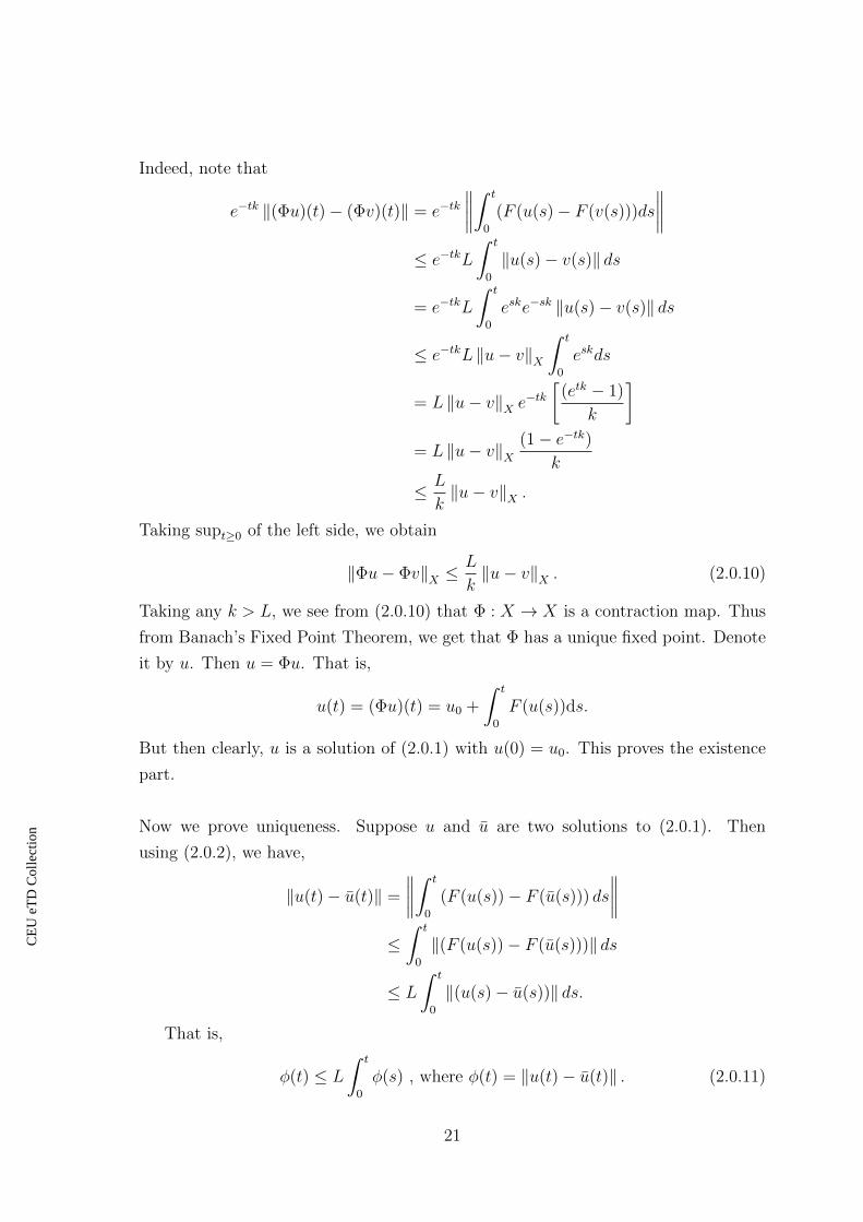
Indeed, note that

e−tk ‖(Φu)(t)− (Φv)(t)‖ = e−tk∥∥∥∥∫ t

0

(F (u(s)− F (v(s)))ds

∥∥∥∥≤ e−tkL

∫ t

0

‖u(s)− v(s)‖ ds

= e−tkL

∫ t

0

eske−sk ‖u(s)− v(s)‖ ds

≤ e−tkL ‖u− v‖X∫ t

0

eskds

= L ‖u− v‖X e−tk[

(etk − 1)

k

]= L ‖u− v‖X

(1− e−tk)k

≤ L

k‖u− v‖X .

Taking supt≥0 of the left side, we obtain

‖Φu− Φv‖X ≤L

k‖u− v‖X . (2.0.10)

Taking any k > L, we see from (2.0.10) that Φ : X → X is a contraction map. Thus

from Banach’s Fixed Point Theorem, we get that Φ has a unique fixed point. Denote

it by u. Then u = Φu. That is,

u(t) = (Φu)(t) = u0 +

∫ t

0

F (u(s))ds.

But then clearly, u is a solution of (2.0.1) with u(0) = u0. This proves the existence

part.

Now we prove uniqueness. Suppose u and u are two solutions to (2.0.1). Then

using (2.0.2), we have,

‖u(t)− u(t)‖ =

∥∥∥∥∫ t

0

(F (u(s))− F (u(s))) ds

∥∥∥∥≤∫ t

0

‖(F (u(s))− F (u(s)))‖ ds

≤ L

∫ t

0

‖(u(s)− u(s))‖ ds.

That is,

φ(t) ≤ L

∫ t

0

φ(s) , where φ(t) = ‖u(t)− u(t)‖ . (2.0.11)

21

CE

UeT

DC

olle

ctio

n

Let f(t) =∫ t

0φ(s)ds. Then f ′(t) = φ(t). Therefore, from (2.0.11), we have

f ′(t) ≤ Lf(t)

⇒f ′(t)− Lf(t) ≤ 0. (2.0.12)

Let h(t) = e−Ltf(t). Then

h′(t) = e−Ltf ′(t)− Le−Ltf(t)

= e−Lt(f ′(t)− Lf(t))

≤ 0.

Thus h(t) is a non-increasing function. So we have

h(t) ≤ 0, for any t ≥ 0

⇒ e−Ltf(t) ≤ 0.

But e−Lt > 0 , so it must be that f(t) ≤ 0. Again,

f(t) =

∫ t

0

φ(s)ds =

∫ t

0

∥∥u(s)− ¯u(s)∥∥ ds ≥ 0.

Therefore, f(t) = 0 for all t ≥ 0. That is,

φ(t) ≤ Lf(t) = 0

⇒ φ(t) = 0, ∀t ≥ 0

⇒ φ ≡ 0.

Thus, we have shown uniqueness of the solution. This concludes our proof.

Now we will go on to state and prove the Hille-Yosida Theorem. Henceforth, by

H, we will denote a real Hilbert space. First we will state and prove the following

lemmas which we will use during the course of the proof.

Lemma 2.1.2. Let w ∈ C1([0,+∞);H) be a function satisfying

dw

dt+ Aλw = 0 on [0,+∞) (2.1.a)

where Aλ = 1λ(I − Jλ) is the Yosida approximation, and Jλ is the resolvent of a

maximal monotone operator A as defined in Section 1.1. Then the functions t 7→|w(t)| and t 7→ |dw

dt(t)| are non-increasing on [0,+∞)

22

CE

UeT

DC

olle

ctio

n

Proof. First note that

d|w(t)|2

dt= lim

h→0

[|w(t+ h)|2 − |w(t)|2

h

]= lim

h→0

1

h[(w(t+ h), w(t+ h))− (w(t), w(t))]

= limh→0

1

h[(w(t+ h), w(t+ h))− (w(t), w(t+ h)) + (w(t+ h), w(t))− (w(t), w(t))]

= limh→0

1

h[(w(t+ h)− w(t), w(t+ h)) + (w(t+ h)− w(t), w(t))]

= limh→0

(w(t+ h)− w(t)

h,w(t+ h)

)+ lim

h→0

(w(t+ h)− w(t)

h,w(t)

)= 2

(dw(t)

dt, w(t)

). (2.1.b)

Since w satisfies (2.1.a), we have(

dw(t)dt

, w(t))

= (−Aλw(t), w(t)) = − (Aλw(t), w(t)).

Recall that (Aλv, v) ≥ 0 for all v ∈ H. Therefore,

d|w(t)|2

dt= − (Aλw(t), w(t))

≤ 0.

That is, |w(t)|2 is an non-increasing function on [0,+∞). Then, |w(t)| = (|w(t)|2)1/2

is also non-increasing on [0,+∞).

Since Aλ is a linear bounded operator we have

d

dt

(dw

dt

)+ Aλ

(dw

dt

)= 0, t ≥ 0. (2.1.e)

So, dw/dt satisfies (2.1.a). Using the same argument as that used in showing |w(t)|is non-increasing, we conclude that |dw/dt| is non-increasing.

Moreover,

d

dt

(dkw

dtk

)+ Aλ

(dkw

dtk

)= 0, t ≥ 0. (for any order k)

This is turn implies |dkwdtk| is non-increasing for any order k.

23

CE

UeT

DC

olle

ctio

n

Lemma 2.1.3. Consider a sequence of functions fn ∈ C1([a, b];H). Suppose the

sequence of functions dfndt

converges uniformly to a function g : [a, b] → H. If fn(t0)

converges for some point t0 on [a, b], then fn converges uniformly to some function,

f(say). Then f is differentiable and dfdt

= g.

Proof. A similar result holds for real valued functions (see Theorem 7.17 in [16]).For

our case, let’s fix some v ∈ H. Denote hn(t) = (fn(t), v); h(t) = (f(t), v); h1(t) =

(g(t), v). Note that h′n(t) = (f ′n(t), v) and these are all scalar functions. So we can

apply Theorem 7.17 ( [16]) to conclude that the sequence of function hn converges

uniformly to the function h(t) = (f(t), v) and h′(t) = h1(t) = (g(t), v),∀t ∈ [a, b].

That is, (f ′(t), v) = (g(t), v). The choice of v ∈ H was arbitrary. Therefore, f ′(t) =

g(t).

Lemma 2.1.4. Let u0 ∈ D(A). Then for any ε > 0, ∃u0 ∈ D(A2) such that |u0−u0| <ε and |Au0 − Au0| < ε. That is, D(A2) is dense in D(A) for the graph norm.

Proof. Take u0 ∈ D(A). Recall that D(Jλ) = H,R(Jλ) = D(A). Denote u0 = Jλu0 =

(I + λA)−1u0. Then u0 ∈ D(A) and u0 = u0 + λAu0.

Therefore, λAu0 = u0 − u0 ∈ D(A) ⇒ Au0 ∈ D(A). But u0 ∈ D(A), Au0 ∈ D(A)

⇒ u0 ∈ D(A2).

Now recall that

Jλ(Av) = Aλv ∀v ∈ D(A),∀ λ > 0

and

A(Jλv) = Aλv ∀v ∈ H,∀ λ > 0

Therefore, ∀ v ∈ D(A), ∀ λ > 0, we have

Jλ(Av) = A(Jλv) (2.1.h)

Also, recall that limλ→0 Jλv = v, ∀ v ∈ H. Therefore,

limλ→0|Jλu0 − u0| = 0

and

limλ→0|Jλ(Au0)− Au0| = 0

24

CE

UeT

DC

olle

ctio

n

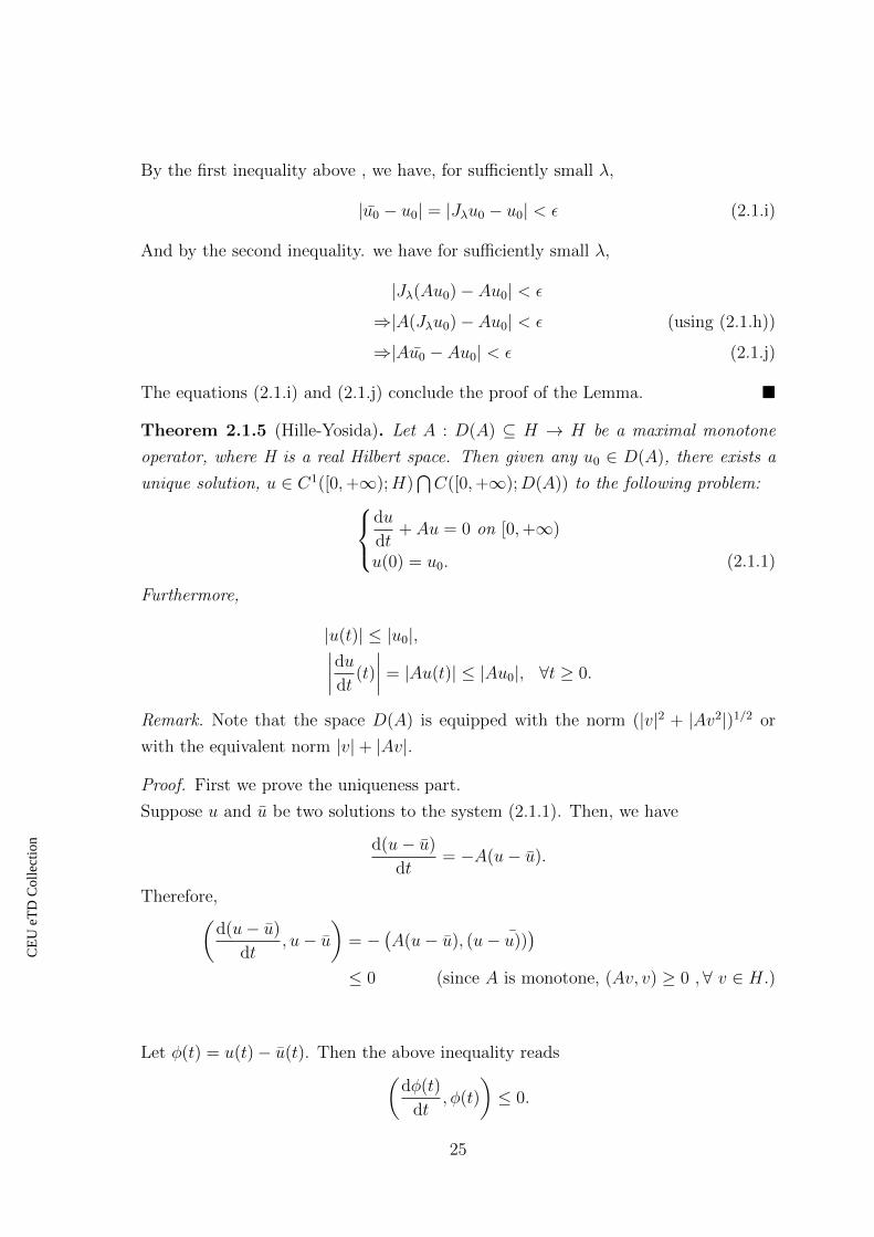
By the first inequality above , we have, for sufficiently small λ,

|u0 − u0| = |Jλu0 − u0| < ε (2.1.i)

And by the second inequality. we have for sufficiently small λ,

|Jλ(Au0)− Au0| < ε

⇒|A(Jλu0)− Au0| < ε (using (2.1.h))

⇒|Au0 − Au0| < ε (2.1.j)

The equations (2.1.i) and (2.1.j) conclude the proof of the Lemma.

Theorem 2.1.5 (Hille-Yosida). Let A : D(A) ⊆ H → H be a maximal monotone

operator, where H is a real Hilbert space. Then given any u0 ∈ D(A), there exists a

unique solution, u ∈ C1([0,+∞);H)⋂C([0,+∞);D(A)) to the following problem:

du

dt+ Au = 0 on [0,+∞)

u(0) = u0. (2.1.1)

Furthermore,

|u(t)| ≤ |u0|,∣∣∣∣dudt (t)

∣∣∣∣ = |Au(t)| ≤ |Au0|, ∀t ≥ 0.

Remark. Note that the space D(A) is equipped with the norm (|v|2 + |Av2|)1/2 or

with the equivalent norm |v|+ |Av|.

Proof. First we prove the uniqueness part.

Suppose u and u be two solutions to the system (2.1.1). Then, we have

d(u− u)

dt= −A(u− u).

Therefore,(d(u− u)

dt, u− u

)= −

(A(u− u), (u− u))

)≤ 0 (since A is monotone, (Av, v) ≥ 0 ,∀ v ∈ H.)

Let φ(t) = u(t)− u(t). Then the above inequality reads(dφ(t)

dt, φ(t)

)≤ 0.

25

CE

UeT

DC

olle

ctio

n

Note that |φ|2 = (φ, φ). We have

d|φ(t)|2

dt= lim

h→0

[|φ(t+ h)|2 − |φ(t)|2

h

]= lim

h→0

1

h[(φ(t+ h), φ(t+ h))− (φ(t), φ(t))]

= limh→0

1

h[(φ(t+ h), φ(t+ h))− (φ(t), φ(t+ h)) + (φ(t+ h), φ(t))− (φ(t), φ(t))]

= limh→0

1

h[(φ(t+ h)− φ(t), φ(t+ h)) + (φ(t+ h)− φ(t), φ(t))]

= limh→0

(φ(t+ h)− φ(t)

h, φ(t+ h)

)+ lim

h→0

(φ(t+ h)− φ(t)

h, φ(t)

)= 2

(dφ(t)

dt, φ(t)

)(2.1.~)

≤ 0.

This means |φ(t)|2 is an non-increasing function on [0,+∞). Then for any t ≥ 0,

|φ(t)|2 ≤ |φ(0)|2 = |u(0)− u(0)|2 = |u0 − u0|2 = 0.

Therefore, |φ(t)| = 0 , for any t ≥ 0. That is, φ ≡ 0. This proves uniqueness.

Now we will prove the Existence part. We will use the following strategy. We re-

place A by Aλ in (2.1.1) and we use Theorem 2.1.1(Cauchy-Picard-Lipschitz) on the

approximate problem. Then using the fact that limλ→0Aλv = Av and a number of

estimates that are independent of λ, we pass on to the limit as λ→ 0+.

Recall that

|Aλv| ≤1

λ|v| ∀ v ∈ H and ∀λ > 0.

That is, Aλ is Lipschitz with Lipschitz constant 1/λ.

Using Theorem 2.1.1, we have that for any λ > 0 there exists a solution (say uλ) of

the problem: dw

dt(t) = −Aλw(t) on [0,+∞),

w(0) = u0 ∈ D(A),

26

CE

UeT

DC

olle

ctio

n

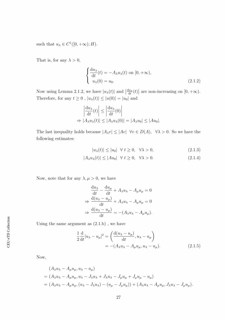
such that uλ ∈ C1([0,+∞);H).

That is, for any λ > 0, duλdt

(t) = −Aλuλ(t) on [0,+∞),

uλ(0) = u0. (2.1.2)

Now using Lemma 2.1.2, we have |uλ(t)| and∣∣duλ

dt(t)∣∣ are non-increasing on [0,+∞).

Therefore, for any t ≥ 0 , |uλ(t)| ≤ |u(0)| = |u0| and∣∣∣∣duλdt(t)

∣∣∣∣ ≤ ∣∣∣∣duλdt(0)

∣∣∣∣⇒ |Aλuλ(t)| ≤ |Aλuλ(0)| = |Aλu0| ≤ |Au0|.

The last inequality holds because |Aλv| ≤ |Av| ∀v ∈ D(A), ∀λ > 0. So we have the

following estimates:

|uλ(t)| ≤ |u0| ∀ t ≥ 0, ∀λ > 0, (2.1.3)

|Aλuλ(t)| ≤ |Au0| ∀ t ≥ 0, ∀λ > 0. (2.1.4)

Now, note that for any λ, µ > 0, we have

duλdt− duµ

dt+ Aλuλ − Aµuµ = 0

⇒ d(uλ − uµ)

dt+ Aλuλ − Aµuµ = 0

⇒ d(uλ − uµ)

dt= −(Aλuλ − Aµuµ).

Using the same argument as (2.1.b) , we have

1

2

d

dt|uλ − uµ|2 =

(d(uλ − uµ)

dt, uλ − uµ

)= −(Aλuλ − Aµuµ, uλ − uµ). (2.1.5)

Now,

(Aλuλ − Aµuµ, uλ − uµ)

= (Aλuλ − Aµuµ, uλ − Jλuλ + Jλuλ − Jµuµ + Jµuµ − uµ)

= (Aλuλ − Aµuµ, (uλ − Jλuλ)− (uµ − Jµuµ)) + (Aλuλ − Aµuµ, Jλuλ − Jµuµ).

27

CE

UeT

DC

olle

ctio

n

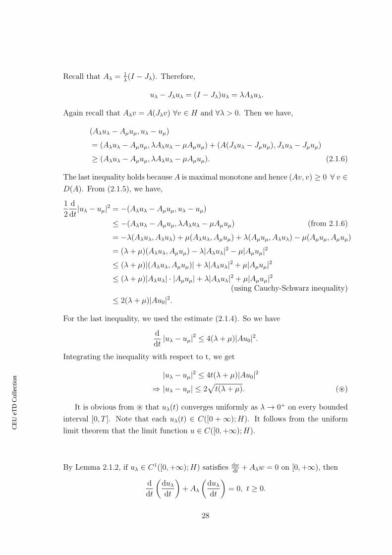
Recall that Aλ = 1λ(I − Jλ). Therefore,

uλ − Jλuλ = (I − Jλ)uλ = λAλuλ.

Again recall that Aλv = A(Jλv) ∀v ∈ H and ∀λ > 0. Then we have,

(Aλuλ − Aµuµ, uλ − uµ)

= (Aλuλ − Aµuµ, λAλuλ − µAµuµ) + (A(Jλuλ − Jµuµ), Jλuλ − Jµuµ)

≥ (Aλuλ − Aµuµ, λAλuλ − µAµuµ). (2.1.6)

The last inequality holds because A is maximal monotone and hence (Av, v) ≥ 0 ∀ v ∈D(A). From (2.1.5), we have,

1

2

d

dt|uλ − uµ|2 = −(Aλuλ − Aµuµ, uλ − uµ)

≤ −(Aλuλ − Aµuµ, λAλuλ − µAµuµ) (from 2.1.6)

= −λ(Aλuλ, Aλuλ) + µ(Aλuλ, Aµuµ) + λ(Aµuµ, Aλuλ)− µ(Aµuµ, Aµuµ)

= (λ+ µ)(Aλuλ, Aµuµ)− λ|Aλuλ|2 − µ|Aµuµ|2

≤ (λ+ µ)|(Aλuλ, Aµuµ)|+ λ|Aλuλ|2 + µ|Aµuµ|2

≤ (λ+ µ)|Aλuλ| · |Aµuµ|+ λ|Aλuλ|2 + µ|Aµuµ|2(using Cauchy-Schwarz inequality)

≤ 2(λ+ µ)|Au0|2.

For the last inequality, we used the estimate (2.1.4). So we have

d

dt|uλ − uµ|2 ≤ 4(λ+ µ)|Au0|2.

Integrating the inequality with respect to t, we get

|uλ − uµ|2 ≤ 4t(λ+ µ)|Au0|2

⇒ |uλ − uµ| ≤ 2√t(λ+ µ). (~)

It is obvious from ~ that uλ(t) converges uniformly as λ→ 0+ on every bounded

interval [0, T ]. Note that each uλ(t) ∈ C([0 +∞);H). It follows from the uniform

limit theorem that the limit function u ∈ C([0,+∞);H).

By Lemma 2.1.2, if uλ ∈ C1([0,+∞);H) satisfies dwdt

+ Aλw = 0 on [0,+∞), then

d

dt

(duλdt

)+ Aλ

(duλdt

)= 0, t ≥ 0.

28

CE

UeT

DC

olle

ctio

n

Also from the proof of Lemma 2.1.2, we have uλ ∈ C∞([0,+∞);H). Let’s denote

vλ = duλdt

, then vλ ∈ C∞([0,+∞);H) and dvλdt

+ Aλvλ = 0 Then

d(vλ − vµ)

dt= −(Aλvλ − Aµvµ).

Using the same argument as (2.1.b), we have

1

2

d

dt|vλ − vµ|2 =

(d(vλ − vµ)

dt, vλ − vµ

)= −(Aλvλ − Aµvµ, vλ − vµ).

Now,

(Aλvλ − Aµvµ, vλ − vµ)

= (Aλvλ − Aµvµ, vλ − Jλvλ + Jλvλ − Jµvµ + Jµvµ − vµ)

= (Aλvλ − Aµvµ, λAλvλ − µAµvµ) + (Aλvλ − Aµvµ, Jλvλ − Jµvµ)(since Aλ = 1/λ(I − Jλ))

= (Aλvλ − Aµvµ, λAλvλ − µAµvµ) + (A(Jλvλ − Jµvµ), Jλvλ − Jµvµ)

≥ (Aλvλ − Aµvµ, λAλvλ − µAµvµ). (since (Av, v) ≥ 0, A being monotone)

Therefore,

1

2

d

dt|vλ − vµ|2

= −(Aλvλ − Aµvµ, λAλvλ − µAµvµ)

≤ |(Aλvλ − Aµvµ, λAλvλ − µAµvµ)|

≤ |Aλvλ − Aµvµ| · |λAλvλ − µAµvµ| (by Cauchy-Schwarz inequality)

≤ (|Aλvλ|+ |Aµvµ|)(λ|Aλvλ|+ µ|Aµvµ|). (2.1.7)

Again from the proof of Lemma 2.1.2,∣∣dvλ

dt

∣∣ =∣∣∣d2uλ

dt2

∣∣∣ is non-increasing on [0,+∞).

Therefore, ∣∣∣∣dvλdt(t)

∣∣∣∣ ≤ |Aλvλ(0)| =∣∣∣∣Aλduλ

dt(0)

∣∣∣∣= |AλAλu0| = |A2

λu0|

⇒ |Aλvλ(t)| ≤ |A2λu0| ∀ λ > 0. (2.1.8)

Now we assume that u0 ∈ D(A2), so, Au0 ∈ D(A). Since Aλv = Jλ(Av), ∀ v ∈D(A), ∀ λ > 0, we have

A2λu0 = Aλ(Aλu0) = Aλ(Jλ(Au0)) = JλA(Jλ(Au0)) = JλJλA(Au0) = J2

λA2u0.

29

CE

UeT

DC

olle

ctio

n

Therefore,

|A2λu0| = |J2

λA2u0| ≤ ‖Jλ‖2

L(H) |A2u0|

≤ |A2u0|. (2.1.9)

The last inequality holds because ‖Jλ‖L(H) ≤ 1 for all λ > 0.

From (2.1.7) and (2.1.8), we have

1

2

d

dt|vλ − vµ|2 ≤ 2|A2

λu0|(λ+ µ)|A2λu0|

= 2(λ+ µ)|A2λu0|2

≤ 2(λ+ µ)|A2u0|2. (from (2.1.9))

Integrating wrt t, we have

|vλ(t)− vµ(t)| ≤ 2√t(λ+ µ)|A2u0|. (2.1.9a)

Therefore vλ → v uniformly on every bounded interval [0, T ] as λ → 0+. Since

vλ ∈ C([0,+∞);H), v being the uniform limit of vλ, satisfies v ∈ C([0, T ];H) for

every T > 0, and hence v ∈ C([0,+∞);H).

So far we have, as λ→ 0+

uλ(t)→ u(t) uniformly on [0, T ]

duλdt

(t)→ v(t) uniformly on [0, T ], ∀ T > 0. (2.1.10)

By Lemma 2.1.3, we have u has a derivative dudt

and v(t) = dudt

(t). Besides , sinceduλdt∈ C([0,+∞);H), and v(t) = du

dt(t) is the uniform limit, it also holds that du

dt∈

C([0,+∞);H). And hence, u ∈ C1([0,+∞);H).

Now note that we can write duλdt

(t) + Aλuλ(t) = 0 as

duλdt

(t) + A(Jλuλ(t)) = 0. (since Aλx = A(Jλx) ∀ x ∈ H, ∀ λ > 0)

30

CE

UeT

DC

olle

ctio

n

Recall that limλ→0 Jλx = x. Therefore

|Jλuλ(t)− u(t)|

≤|Jλuλ(t)− Jλu(t)|+ |Jλu(t)− u(t)|

≤ ‖Jλ‖L(H) |uλ(t)− u(t)|+ |Jλu(t)− u(t)|

→0 as λ→ 0+

That is,

Jλuλ(t)→ u(t) as λ→ 0+. (2.1.11)

Again, from (2.1.10) and (2.1.11),

A(Jλuλ(t)) = −duλdt

(t)→ −du

dtas λ→ 0+.

Since A is closed, this means u(t) ∈ D(A) and

−du

dt(t) = Au(t)

⇒du

dt(t) + Au(t) = 0.

Furthermore, note that since u ∈ C1([0,+∞);H), Au(t) = −dudt∈ C([0,+∞);H). It

follows that

|u(t)− u(t0)|D(A) = |u(t)− u(t0)|+ |Au(t)− Au(t0)|

→ 0 as t→ t0 for all t0 ≥ 0

Thus, u ∈ C([0,+∞);D(A)). Moreover, recall that from the derived estimates (2.1.3)

and (2.1.4), we have

|uλ(t)| ≤ |u0| ∀ t ≥ 0, ∀λ > 0,

|Aλuλ(t)| ≤ |Au0| ∀ t ≥ 0, ∀λ > 0.

And passing on to the limit as λ→ 0+, we have

|u(t)| ≤ |u0| ∀ t ≥ 0,

|Au(t)| ≤ |Au0| ∀ t ≥ 0.

Now note that by Lemma 2.1.4, D(A2) is dense in D(A). Therefore, for any u0 ∈D(A), we can find a sequence (u0n) ⊆ D(A2) such that |u0n − u0|D(A) → 0. That is,

|u0n − u0|+ |Au0n − Au0| → 0.

31

CE

UeT

DC

olle

ctio

n

That is, u0n → u0 and Au0n → Au0. By the preceding analysis, for every u0n ∈ D(A2),

we know that the problem: dw

dt+ Aw = 0 on [0,+∞),

w(0) = u0n,

has a solution , say, un which satisfies

|un(t)| ≤ |u0|∣∣∣∣dundt(t)

∣∣∣∣ = |Aun(t)| ≤ |Au0| ∀ t ≥ 0.

Note that un − um is a solution to the problemdw

dt+ Aw = 0 on [0,+∞),

w(0) = u0n − u0m,

therefore, for all t ≥ 0, we have

|un(t)− um(t)| ≤ |u0n − u0m|, (2.1.12)∣∣∣∣dundt(t)− dum

dt(t)

∣∣∣∣ ≤ |Au0n − Au0m|. (2.1.13)

Since u0n → u0 in H, (u0n) is a Cauchy sequence in H. Therefore given any ε > 0 for

sufficiently large m,n, we have

|un(t)− um(t)| ≤ |u0m − u0n| < ε

That is, (un(t)) is a Cauchy sequence in H. Thus (un(t)) has a pontwise limit in H.

Let’s denote it as u(t) := limn→∞ un(t). Then from (2.1.12),

limm→∞

|un(t)− um(t)| ≤ limm→∞

|u0n − u0m|

⇒|un(t)− u(t)| ≤ |u0n − u0|

Therefore, for any T ≥ 0

supt∈[0,T ]

|un(t)− u(t)| ≤ |u0n − u0|

→ 0 as n→∞.

Thus,

un(t)→ u(t) uniformly on [0, T ] ∀ T ≥ 0. (2.1.14)

32

CE

UeT

DC

olle

ctio

n

By a similar argument, we have from (2.1.13) ,

dundt

(t)→ φ(t) uniformly on [0, T ] ∀ T ≥ 0 (2.1.15)

where φ(t) is the pointwise limit of dundt

(t). Therefore by Lemma 2.1.3, it follows that

u(t) is differentiable and φ(t) = dudt

(t) on [0, T ] for any T ≥ 0. Since un are continuous

on [0, T ], so is the uniform limit u on [0, T ] ∀ T ≥ 0. That is, u ∈ C([0,+∞);H).

Again, since un ∈ C1([0,+∞);H), it follow that dundt

(t) ∈ C([0,+∞);H), and thus,dudt

(t) being the uniform limit , it follows that dudt

(t) is continuous on [0, T ] ∀ T ≥ 0.

That is, dudt

(t) ∈ C([0,+∞);H). Hence,

u ∈ C1([0,+∞);H).

Now, we note that

Aun(t) = −dundt

(t)→ −du

dt(t)

and

un(t)→ u(t).

But since A is a closed operator, it follows that u(t) ∈ D(A) and Au(t) = −dudt

(t),

that is,du

dt(t) + Au(t) = 0.

Moreover, note that Au = −dudt∈ C([0,+∞);H). Also since u ∈ C1([0,+∞);H), we

have

|u(t)− u(t0)|D(A)

= |u(t)− u(t0)|+ |Au(t)− Au(t0)|

→ 0 as |t− t0| → 0 for any t0 ≥ 0.

Thus,

u ∈ C([0,+∞);D(A)).

This concludes the proof of the Theorem.

2.2 Regularity of the solutions

It turns out that if one were to make additional assumptions on the initial data

u0, the solution to the system (2.1.1) in Theorem 2.1.5 (Hille-Yosida Theorem) is

33

CE

UeT

DC

olle

ctio

n

more regular than just C1([0,+∞);H)⋂C([0,+∞);D(A)). For that purpose we

inductively define the space D(Ak) = v ∈ D(Ak−1);Av ∈ D(Ak−1), where k ≥ 2 is

an integer.

Claim : D(Ak) is a Hilbert space for the scalar product

(u, v)D(Ak) =k∑j=0

(Aju,Ajv);

the corresponding norm is

|u|D(Ak) =

(k∑j=0

|Aju|2) 1

2

.

Proof. Note that (u, v)D(Ak) being a finite sum of scalar products is indeed a scalar

product itself. Let (un) ⊆ D(Ak) be a Cauchy sequence. That is, given ε > 0, ∃ Nε

such that ∀ m,n > Nε,

|un − um|D(Ak) < ε

⇒

(k∑j=0

|Aj(un − um)|2) 1

2

< ε

⇒ |un − um|2 + |Aun − Aum|2 + · · ·+ |Akun − Akum|2 < ε2 ∀ m,n > Nε

⇒ |un − um|2 < ε2

⇒ |un − um| < ε

This means un is also Cauchy in H. Then un converges to some limit u0 ∈ H. Similarly,

(Aun), (A2un), · · · , (Akun) are Cauchy sequences in H and hence they converge to the

limits, say u1, u2, · · · , uk respectively.

Recall that A is maximal monotone and hence a closed operator. Note that

(un) ⊂ D(Ak) implies (un) ⊂ D(Aj) for j = 0 to k. Now (un) ⊂ D(A), un → u0 ∈ H,

Aun → u1 ∈ H. Since A is closed, this means u0 ∈ D(A) and u1 = Au0.

Again, (un) ⊂ D(A2) and we just saw that Aun → Au0. Also, A(Aun) = A2un → u2

Since A is closed, it follows that Au0 ∈ D(A) and u2 = A2u0.

Repeating this argument inductively, it is clear that uj = Aju0 and Aju0 ∈ D(A)

for j = 0 to k. This in turn implies that u0 ∈ D(Ak). Thus the Cauchy sequence

(un)→ u0 in D(Ak) and hence D(Ak) is complete wrt the distance function induced

by the scalar product.

34

CE

UeT

DC

olle

ctio

n

Theorem 2.2.1. Suppose u0 ∈ D(Ak) for some integer k ≥ 2. Then the solution u

to the problem (2.1.1): du

dt+ Au = 0 on [0,+∞),

u(0) = u0,

satisfies

u ∈ Ck−j([0,+∞);D(Aj)) ∀ j = 0, 1, · · · , k.

Proof. Assume first k = 2. Denote by H1 the Hilbert space D(A) equipped with the

scalar product (u, v)D(A) = (u, v) + (Au,Av) and the norm |u|D(A) = (|u|2 + |Au|2)1/2.

Denote by A1 the operator A1 : D(A1) ⊂ H1 → H1 such that

D(A1) = D(A2),

A1v = Av for v ∈ D(A1) = D(A2).

We will show that A1 is maximal monotone in H1 = D(A).

Note that for v ∈ D(A1) = D(A2) ⊂ D(A), (A1v, v) = (Av, v) ≥ 0. Now, take

any f ∈ H1 = D(A). Since A is maximal monotone, this means ∃ u ∈ D(A) = H1

such that u+ Au = f . That is, Au = f − u. Now f, u ∈ H1 ⇒ Au = f − u ∈ H1.

But u ∈ D(A) and Au ∈ D(A) imply u ∈ D(A2). Thus for any f ∈ H1, we have

found u ∈ D(A1) such that u + A1u = u + Au = f . So A1 is maximal monotone in

H1.

Consider the system du

dt+ A1u = 0 on [0,+∞),

u(0) = u0, (2.2.1)

with maximal monotone operator A1 in the space H1. So we can apply Theorem 2.1.5

to the above system to obtain a solution u ∈ C1([0,+∞);H1)⋂C([0,+∞);D(A1)).

Note that u(t) ∈ D(A1) = D(A2) ⊂ D(A). So A1u(t) = Au(t). But then u satisfiesdu

dt+ Au = 0 on [0,+∞),

u(0) = u0.

By the uniqueness of the solution obtained in Theorem 2.1.5, this u is the unique

solution to the system (2.1.1).

35

CE

UeT

DC

olle

ctio

n

So we have that u ∈ C1([0,+∞);D(A))⋂C([0,+∞);D(A2)). Now we will show

that u ∈ C2([0,+∞);H).

For any x ∈ H1 with |x|H1 = 1, we have

|x|H1 = (x, x)H1 = 1

⇒ |x|2 + |Ax|2 = 1

⇒ |x|2 = 1− |Ax|2 ≤ 1.

This is true for all x ∈ H1 such that |x|H1 = 1. So, |Ax| ≤ 1, ∀ x ∈ H1 such that

|x|H1 = 1 and therefore

supx ∈ H1|x|H1

= 1

|Ax| ≤ 1.

That is, when A is considered as an operator from H1(as a Hilbert space with

(·, ·)H1), it is a a bounded linear operator(hence continuous). In other words,

A ∈ L(H1;H)

Again, we have from before that u ∈ C([0,+∞);H1). Therefore Au ∈ C([0,+∞);H).

We had previously shown that u ∈ C([0,+∞);D(A1)). Therefore,

u ∈ C([0,+∞);D(A1))

⇒ u(t) ∈ D(A1) = D(A2)

⇒ Au(t) ∈ D(A)

⇒ − du

dt(t) ∈ D(A) = H1.

36

CE

UeT

DC

olle

ctio

n

Now,

limh→0

Au(t+ h)− Au(t)

h

= limh→0

A

(u(t+ h)− u(t)

h

)=A

(limh→0

u(t+ h)− u(t)

h

)(since A is linear bdd, hence continuous)

=A

(du

dt

)∴

d

dt(Au) = A

(du

dt

)(2.2.2)

∴d

dt

(du

dt

)=

d

dt(−Au)

=− A(

du

dt

).

Therefore,

d

dt

(du

dt

)= −A

(du

dt

)∈ C([0,+∞);H)

⇒ du

dt∈ C1(0,+∞];H)

⇒ u ∈ C2([0,+∞];H).

Also,

d

dt

(du

dt

)= −A

(du

dt

)⇒ d

dt

(du

dt

)+ A

(du

dt

)= 0 on [0,+∞). (2.2.3)

Now we use induction for the general case k ≥ 3. Assume the Theorem holds up to

order k − 1. Suppose u0 ∈ D(Ak). We have shown above that the solution u of the

problem du

dt+ Au = 0 on [0,+∞),

u(0) = u0.

37

CE

UeT

DC

olle

ctio

n

satisfies :

u ∈ C2([0,+∞);H)⋂

C1([0,+∞);D(A)),

d

dt

(du

dt

)+ A

(du

dt

)= 0 on [0,+∞).

Let’s denote v = dudt

. Note that v satisfies the system:

dv

dt+ Av = 0 on [0,+∞),

v(0) =du

dt(0) = −Au(0) = −Au0. (2.2.4)

By assumption, u0 ∈ D(Ak). So −Au0 ∈ D(Ak−1). By Induction hypothesis the

theorem holds for the system (2.2.4) with v(0) = −Au0 ∈ D(Ak−1). Then

v ∈ Ck−1−j([0,+∞);D(Aj)) for j = 0, 1, · · · , k − 1

⇒ du

dt∈ Ck−1−j([0,+∞);D(Aj)) for j = 0, 1, · · · , k − 1

⇒ u ∈ Ck−j([0,+∞);D(Aj)) for j = 0, 1, · · · , k − 1.

Now we only need to verify that u ∈ C([0,+∞);D(Ak)). For j = k − 1, we have

u ∈ C1([0,+∞);D(Ak−1)

⇒ du

dt∈ C([0,+∞);D(Ak−1))

⇒ Au ∈ C([0,+∞);D(Ak−1)).

So, we have, u(t) ∈ D(Ak−1) and Au(t) ∈ D(Ak−1). Therefore, u(t) ∈ D(Ak) for

all t ≥ 0. Note that

|u(t)− u(t0)|2D(Ak) =k∑j=0

|Aj(u(t)− u(t0))|2 for any t0 ≥ 0.

And,

|Au(t)− Au(t0)|D(Ak−1) =k−1∑j=0

|Aj(Au(t)− Au(t0))|2

=k∑j=1

|Aj(u(t)− u(t0))|2 for any t0 ≥ 0.

38

CE

UeT

DC

olle

ctio

n

Therefore,

|u(t)− u(t0)|D(Ak) =(|u(t)− u(t0)|2 + |Au(t)− Au(t0)|2D(Ak−1

)1/2

⇒ limt→t0|u(t)− u(t0)|D(Ak) =

(limt→t0|u(t)− u(t0)|2 + lim

t→t0|Au(t)− Au(t0)|2

)1/2

= 0(since u ∈ C([0,+∞);H) and Au ∈ C([0,+∞);D(Ak−1)).)

Therefore, u ∈ C([0,+∞);D(Ak)). This concludes the proof.

2.3 The case of self-adjoint operators

Suppose A : D(A) ⊆ H → H is an unbounded linear operator and D(A) is dense in

H, that is, D(A) = H. Define D(A∗) to be the set of all f ∈ H such that the linear

functional g 7→ (f, Ag) extends to a bounded linear functional on all of H. Since

D(A) is dense in H, by Riesz representation theorem it follows that there exists a

unique h ∈ H such that (f, Ag) = (h, g). We define the adjoint operator, A∗ of A

as A∗f = h. Clearly, A∗ is also a linear operator.

An operator A is called symmetric if (u,Av) = (Au, v) ∀ u, v ∈ D(A). An operator

A is called self-adjoint if D(A) = D(A∗) and A = A∗.

Claim 1: A is a symmetric operator if and only if

D(A) ⊆ D(A∗),

A = A∗ on D(A).

Proof. (⇒ :)

A is symmetric. That is, (u,Av) = (Au, v) for all u, v ∈ D(A). Take f ∈ D(A)

and the functional g 7→ (f, Ag). Now, since A is symmetric, (f, Ag) = (Af, g) for all

g ∈ D(A). Denote by T the functional:

T (g) = (Af, g) ∀ g ∈ H.

39

CE

UeT

DC

olle

ctio

n

Note that for g ∈ D(A), T (g) = (Af, g) = (g, Af). And thus T is an extension of the

functional g 7→ (f, Ag) on all of H. Also, note that |(Af, g)| ≤ |Af ||g| by Cauchy-

Schwarz inequality. Hence, T is a bounded linear functional that is an extension of

the functional g 7→ (f, Ag) on all of H. Therefore by definition of D(A∗), f ∈ D(A∗).

The choice of f ∈ D(A) was arbitrary. So, we have D(A) ⊆ D(A∗).

Again, by Riesz’s Representation Theorem, ∃ h ∈ H such that T (g) = (h, g) for

all g ∈ H. By definition, A∗f = h. But T (g) = (Af, g) ∀g ∈ H. Therefore,

(Af, g) = (A∗f, g) ∀ g ∈ H

⇒ Af = A∗f.

This is true for any f ∈ D(A). Therefore, A = A∗ on D(A).

(⇐ : )

We have

D(A) ⊆ D(A∗),

A = A∗ on D(A).

Take any u ∈ D(A). Then u ∈ D(A∗). Then by definition of D(A∗), the functional

g 7→ (u,Ag) can be extended to a bounded linear functional T on all of H such that

T (g) = (A∗u, g) ∀ g ∈ H.

Now A = A∗ ⇒ T (g) = (Au, g) ∀ g ∈ H. So, for g ∈ D(A),

T (g) = (u,Ag) (since T is an extension of the functional)

⇒ (Au, g) = (u,Ag).

Therefore, A is symmetric.

Claim 2: If A is a self-adjoint operator, then it is symmetric.

Proof. A is self-adjoint. Therefore, D(A∗) = D(A) and A = A∗. Take any u ∈D(A) = D(A∗). By definition of D(A∗), the functional g 7→ (u,Ag) extends to

bounded linear functional, say T on all of H. Then T (g) = (A∗u, g) = (Au, g) for all

g ∈ H. But since T is an extension , for all g ∈ D(A) , (u,Ag) = T (g) = (Au, g).

Thus for all u, g ∈ D(A), (u,Ag) = (Au, g). That is, A is symmetric.

40

CE

UeT

DC

olle

ctio

n

Claim 3: Suppose T ∈ L(H;H). Then T is symmetric if and only if it’s self-adjoint.

Proof. From Claim 2, we know that a self-adjoint operator is always symmetric. So

we only need to prove (⇒ :)

T is symmetric. Therefore, (u, Tv) = (Tu, v) for all u, v ∈ H. Then from Claim 1,

we have, D(T ) ⊆ D(T ∗). That is, H = D(T ) = D(T ∗) ⊆ H. Therefore, D(T ) =

D(T ∗) = H and T = T ∗ on D(T ) = H. Therefore, T is self-adjoint.

Theorem 2.3.1. Suppose A is a maximal monotone operator that is symmetric.

Then A is self-adjoint.

Proof. Denote J1 = (I + A)−1. Recall that D(J1) = H, R(J1) = D(A), and

‖J1‖L(H) ≤ 1. We will first show that J1 is self-adjoint. Since J1 is linear and

bounded, by Claim 3, it suffices to show that J1 is symmetric.

Take any u, v ∈ H. Denote J1u = u1, J1v = v1.Note that u1, v1 ∈ D(A). Then

u = u1 + Au1, v = v1 + Av1. So, Au1 = u − u1, Av1 = v − v1. A is symmetric.

Therefore,

(u1, Av1) = (Au1, v1)

⇒ (u1, v − v1) = (u− u1, v1)

⇒ (u1, v)− (u1, v1) = (u, v1)− (u1, v1)

⇒ (J1u, v) = (u, J1v)

Thus J1 is symmetric and hence, self-adjoint.

Take any u ∈ D(A∗). Let f = u+A∗u, that is, f −u = A∗u. Recall that from the

definition of adjoint operator, we have (u,Ag) = (A∗u, g) for all g ∈ D(A). Therefore,

(u,Ag) = (f − u, g) = (f, g)− (u, g), that is

(u, g + Ag) = (f, g) ∀ g ∈ D(A). (2.3.1)

41

CE

UeT

DC

olle

ctio

n

Recall that D(J1) = H,R(J1) = D(A). Take any w ∈ H. Then J1w ∈ D(A). Denote

v = J1w. Then v + Av = w. Therefore, by (2.3.1),

(u, v + Av) = (f, v)

⇒ (u,w) = (f, J1w) ∀ w ∈ H.

Since we showed that J1 is symmetric, we have

(f, J1w) = (J1f, w) = (u,w) ∀ w ∈ H.

Taking w = J1f − u,

(J1f, J1f − u) = (u, J1f − u)

⇒ (J1f − u, J1f − u) = 0

⇒ J1f = u.

Therefore, u ∈ R(J1) = D(A). Since the choice of u ∈ D(A∗) was arbitrary, this

means, D(A∗) ⊆ D(A). Again, since A is symmetric, by Claim 1,

D(A) ⊆ D(A∗),

A = A∗ on D(A).

Therefore, D(A) = D(A∗) and A = A∗ on D(A) = D(A∗). Hence, A is self-adjoint.

Theorem 2.3.2. Suppose A is a maximal monotone operator that is self-adjoint.

Then for any u0 ∈ H, ∃ a unique solution

u ∈ C([0,+∞);H) ∩ C1((0,+∞);H) ∩ C((0,+∞);D(A))

to the problem: du

dt+ Au = 0 on (0,+∞),

u(0) = u0. (2.3.2)

Furthermore, we have the following estimates:

|u(t)| ≤ |u0| ∀ t > 0,∣∣∣∣dudt (t)

∣∣∣∣ = |Au(t)| ≤ 1

t|u0| ∀ t > 0,

u ∈ Ck((0,+∞);D(Al)) for all non-negative integers k, l.

42

CE

UeT

DC

olle

ctio

n

Proof. First we show uniqueness. Suppose u and u are two solutions to the system

(2.3.2). We have

du

dt− du

dt+ Au− Au = 0 on (0,+∞)

⇒ d(u− u)

dt= −A(u− u)

⇒(

d(u− u)

dt, u− u

)= −(A(u− u), u− u)

≤ 0. (since A is monotone, (Av, v) ≥ 0, ∀ v ∈ D(A))

Denote φ(t) = u(t)− u(t). Then similar to (2.1.~ ), we get

d

dt|φ(t)|2 = 2

(dφ(t)

dt, φ(t)

)=

(d(u− u)

dt, u− u

)≤ 0 on (0,+∞).

Therefore, |φ|2 is non-increasing on (0,+∞). Since u, u ∈ C([0,+∞);H), φ = u− uis continuous on [0,+∞). Therefore,

|φ(t+ h)|2 ≤ |φ(h)|2 for h ≥ 0,∀ t ≥ 0

⇒ |φ(t)|2 ≤ |φ(0)|2 = 0,∀t ≥ 0

⇒ φ ≡ 0 on [0,+∞).

Thus the solution to (2.3.2) is unique.

Now we prove the existence part. Let us first assume that u0 ∈ D(A2) (that is

u0 ∈ D(A), Au0 ∈ D(A)). Let u be the solution to the system:du

dton [0,+∞),

u(0) = u0,

obtained in Theorem 2.1.5. We will show that∣∣du

dt

∣∣ ≤ 1t|u0| ∀ t > 0. Recall that

Jλ = (I + λA)−1 has D(Jλ) = H and Aλ = 1λ(I − Jλ) has D(Aλ) = D(Jλ) = H.

43

CE

UeT

DC

olle

ctio

n

We showed in the proof of Theorem 2.3.1 that J1 is symmetric. By a similar argument

it follows that Jλ is symmetric and hence by Claim 3, that Jλ is self-adjoint, that is,

Jλ = J∗λ. Now,

(Aλu, v) = (1

λ(I − Jλ)u, v)

=1

λ(u, v)− 1

λ(Jλu, v)

=1

λ(u, v)− 1

λ(u, Jλv) (since Jλ is symmetric)

=

(u,

1

λ(v − Jλv)

)= (u,Aλv).

Thus Aλ is symmetric and hence by Claim 3, it is self-adjoint as well, that is, A∗λ = Aλ.

Consider the following approximate problem that was used in the proof of Theorem

2.1.5: duλdt

+ Aλuλ = 0 on [0,+∞),

u(0) = u0. (2.3.3)

Recall that Aλ is Lipschitz, since |Aλv| ≤ 1λ|v|, ∀ v ∈ H,∀ λ > 0. Then by

Theorem 2.1.1(Cauchy-Lipschitz-Picard), the unique solution uλ to (2.3.3) satisfies

uλ ∈ C1([0,+∞);H). Now from (2.3.3),

duλdt

= −Aλuλ

⇒(

duλdt

(t), uλ(t)

)= −(Aλuλ(t), uλ(t)).

Again, similar to (2.1.~), we have,

1

2

d

dt|uλ(t)|2 =

(duλdt

(t), uλ(t)

)= −(Aλuλ(t), uλ(t)).

Integrating wrt to t over [0, T ], we get

1

2(|uλ(T )|2 − |uλ(0)|2) = −

∫ T

0

(Aλuλ(t), uλ(t))dt

⇒ 1

2|uλ(T )|2 +

∫ T

0

(Aλuλ(t), uλ(t))dt =|u0|2

2. (2.3.4)

Taking the scalar product of (2.3.3) with tdudt

, we have

t

∣∣∣∣duλdt

∣∣∣∣2 + t

(Aλuλ(t),

duλdt

(t)

)= 0.

44

CE

UeT

DC

olle

ctio

n

Integrating wrt to t over [0, T ], we get∫ T

0

∣∣∣∣duλdt(t)

∣∣∣∣2 tdt+

∫ T

0

(Aλuλ(t),

duλdt

(t)

)tdt = 0. (2.3.5)

Now,

d

dt(Aλuλ, uλ)

= limh→0

(Aλuλ(t+ h), uλ(t+ h))− (Aλuλ(t), uλ(t))

h

= limh→0

(Aλuλ(t+ h)− Aλuλ(t), uλ(t+ h))− (Aλuλ(t), uλ(t+ h)− uλ(t))h

= limh→0

(Aλ

(uλ(t+ h)− uλ(t)

h

), uλ(t+ h)

)+ lim

h→0

(Aλuλ(t),

uλ(t+ h)− uλ(t)h

)=

(Aλ

duλdt

, uλ

)+

(Aλuλ,

duλdt

)=

(duλdt

, Aλuλ

)+

(Aλuλ,

duλdt

)(since Aλ is self-adjoint)

= 2

(Aλuλ,

duλdt

). (2.3.6)

From (2.3.6), ∫ T

0

(Aλuλ,

duλdt

)tdt

=1

2

∫ T

0

[d

dt(Aλuλ, uλ)

]tdt

=1

2

[t

∫d

dt(Aλuλ, uλ)dt

]T0

− 1

2

∫ T

0

(∫d

dt(Aλuλ, uλ)dt

)dt

(using integration by parts)

=T

2(Aλuλ(T ), uλ(T ))− 1

2

∫ T

0

(Aλuλ, uλ)dt. (2.3.7)

By Lemma 2.1.1, t 7→∣∣duλ

dt(t)∣∣ is non-increasing. Therefore,∫ T

0

∣∣∣∣duλdt(t)

∣∣∣∣2 tdt ≥ ∣∣∣∣duλdt(T )

∣∣∣∣2 ∫ T

0

tdt =

∣∣∣∣duλdt(T )

∣∣∣∣2 T 2

2. (2.3.8)

45

CE

UeT

DC

olle

ctio

n

From (2.3.7), we have∫ T

0

(Aλuλ, uλ)dt

= T (Aλuλ(T ), uλ(T ))− 2

∫ T

0

(Aλuλ,

duλdt

)tdt

= T (Aλuλ(T ), uλ(T )) + 2

∫ T

0

∣∣∣∣duλdt

∣∣∣∣2 tdt (using (2.3.5))

≥ T (Aλuλ(T ), uλ(T )) + T 2

∣∣∣∣dudt (T )

∣∣∣∣2 . (using (2.3.8))

So, ∫ T

0

(Aλuλ, uλ)dt ≥ T (Aλuλ(T ), uλ(T )) + T 2

∣∣∣∣dudt (T )

∣∣∣∣2 . (2.3.9)

Now, from (2.3.4),

|u0|2

2=

1

2|uλ(T )|2 +

∫ T

0

(Aλuλ, uλ)dt

≥ 1

2|uλ(T )|2 + T (Aλuλ(T ), uλ(T )) + T 2

∣∣∣∣duλdt(T )

∣∣∣∣2 . (using (2.3.9))

That is,

|uλ(T )|2 + 2T (Aλuλ(T ), uλ(T )) + 2T 2

∣∣∣∣duλdt(T )

∣∣∣∣2 ≤ |u0|2

⇒ |uλ(T )|2 + 2T (Aλuλ(T ), uλ(T )) + T 2

∣∣∣∣duλdt(T )

∣∣∣∣2 + T 2

∣∣∣∣duλdt(T )

∣∣∣∣2 ≤ |u0|2

⇒ |uλ(T )|2 + 2T (Aλuλ(T ), uλ(T )) + T 2|Aλuλ(T )|2 + T 2

∣∣∣∣duλdt(T )

∣∣∣∣2 ≤ |u0|2

(using duλ/dt = −Aλuλ)

⇒∣∣∣∣uλ(T ) + T

duλdt

(T )

∣∣∣∣2 + T 2

∣∣∣∣duλdt(T )

∣∣∣∣2 ≤ |u0|2

⇒ T 2

∣∣∣∣duλdt(T )

∣∣∣∣2 ≤ |u0|2

⇒∣∣∣∣duλdt

(T )

∣∣∣∣ ≤ 1

T|u0|, ∀ T > 0, ∀ λ > 0. (2.3.10)

Recall that in the proof of Theorem 2.1.5, we showed that

duλdt→ du

dtuniformly as λ→ 0+.

46

CE

UeT

DC

olle

ctio

n

So, passing on to the limit as λ→ 0+, we get∣∣∣∣dudt (T )

∣∣∣∣ ≤ 1

T|u0| ∀ T > 0.

Recall from Lemma 2.1.4, we have D(A2) is dense in D(A). But here we also have

D(A) is dense in H. So, D(A2) is dense in H. Therefore for any u0 ∈ H, there exists

a sequence (u0n) ⊆ D(A2) such that u0n → u0. Now consider the problem:dw

dt+ Aw = 0 on [0,+∞),

w(0) = u0n.

Thus by Theorem 2.1.5, the above problem has a solution, say un that satisfies un ∈C1([0,+∞);H)

⋂C([0,+∞);D(A)) and furthermore , we have the estimate |un(t)| ≤

|u0|, ∀ t ≥ 0. Also from the preceding analysis, we have∣∣dun

dt(t)∣∣ ≤ 1

t|u0n| , ∀ t > 0.

Note that un − um is a solution to the problem:dw

dt+ Aw = 0,

w(0) = u0n − u0m.

And thus, we have the estimates:∣∣∣∣dundt(t)− dum

dt(t)

∣∣∣∣ ≤ 1

t|u0n − u0m|, t > 0, (2.3.11)

|un(t)− um(t)| ≤ |u0n − u0m|, t ≥ 0. (2.3.12)

Thus un → u uniformly on [0, T ] for every T ≥ 0. Note that un ∈ C1([0,+∞);H),

and hence, u being the uniform limit is also continuous on [0, T ] , ∀t ≥ 0. That is,

u ∈ C([0,+∞);H). From (2.3.11) and Lemma 2.1.3, we see that u is differentiable

on [δ, T + δ] and dundt→ du

dtin C([δ, T + δ];H) for any δ > 0 and T > 0. Hence

du

dt(t) ∈ C((0,+∞);H).

This along with u ∈ C([0,+∞);H) implies that u ∈ C1((0,+∞);H). So,

u ∈ C([0,+∞);H)⋂

C1((0,+∞);H). (2.3.14)

47

CE

UeT

DC

olle

ctio

n

Again, note that

Aun(t) = −dundt

(t)→ −du

dt(t)

and

un(t)→ u(t).

Since A is a closed operator (being maximal monotone), this means

u(t) ∈ D(A) and Au(t) = −du

dt(t),

⇒ du

dt(t) + Au(t) = 0 on (0,+∞).

Now we will prove that u ∈ Ck((0,+∞);D(Al)) for all non-negative integers k, l.

For that, we will first show that

u ∈ Ck−j((0,+∞);D(Aj)) ∀ j = 0, 1, · · · , k for all integers k ≥ 2. (2.3.15)

From (2.3.14), we have,

|u(t)− u(t0)|D(A)

= (|u(t)− u(t0)|2 + |Au(t)− Au(t0)|2)1/2

→ 0 as |t− t0| → 0, ∀ t0 > 0.

This along with (2.3.14) shows that (2.3.15) holds for k = 1. We will proceed by

induction on k. Now assume (2.3.15) holds for all non-negative integers upto k − 1.

Recall that we have already proved the first part of the Theorem , that is, given

any u0 ∈ H, the problem: du

dt+ Au = 0 on (0,+∞),

u(0) = u0

has a unique solution u ∈ C([0,+∞);H)⋂C1((0,+∞);H)

⋂C((0,+∞);D(A)), where

A is a maximal monotone and self-adjoint operator.

Now, let us denote, the Hilbert space H = D(Ak−1) with the norm we introduced

in Section 2.3. Let’s define the operator A as follows:

A : D(A) ⊆ H → H such that

D(A) = D(Ak),

A = A on D(A).

48

CE

UeT

DC

olle

ctio

n

We claim that A is maximal monotone in H. For all v ∈ D(A) = D(Ak), we have

(Av, v)H

= (Av, v)D(Ak−1)

=k−1∑j=0

(Aj(Av), Ajv)

=k−1∑j=0

(A(Ajv), Ajv) (since A = A on D(A))

≥ 0. (since A is monotone)

Now, take any f ∈ H = D(Ak−1). Then f is also in H. Since A is maximal

monotone, we have R(I + A) = H. That is, ∃ v ∈ D(A) such that v + Av = f .

f ∈ D(Ak−1) ⊆ D(A) and v ∈ D(A) imply Av = f − v ∈ D(A). Therefore,

v ∈ D(A2). Proceeding with this same line of argument inductively, it follows that

v ∈ D(Ak−1), and together with f ∈ D(Ak−1), this means Av = f − v ∈ D(Ak−1),

that is, v ∈ D(Ak) = D(A).

Thus for any f ∈ H, ∃v ∈ D(A), such that (I + A)v = f , that is, R(I + A) = H.

So, A is maximal monotone.

Also, note that for all u, v ∈ D(A) = D(Ak), (Au, v) = (Au, v) = (u,Av) =

(u, Av), since A is symmetric and A = A on D(A). Thus A is symmetric.

So by Theorem 2.3.1, A being maximal monotone and symmetric, is also self-

adjoint. Then by the first part of the Theorem, it follows that for any v0 ∈ H, the

system: dv

dt+ Av = 0,

v(0) = v0 (2.3.16)

has a unique solution v ∈ C([0,+∞); H)⋂C1((0,+∞); H)

⋂C((0,+∞);D(A)).

Note that by the induction hypothesis, the solution u of the first part of the

theorem satisfies u(ε) ∈ D(Ak−1) ∀ε > 0. Denote uε(t) = u(t + ε) for t > 0. Then

putting v(0) = u(ε), we see that uε(t) is the unique solution to the system (2.3.16) ,

and hence uε ∈ C([0,+∞); H)⋂C1((0,+∞); H)

⋂C((0,+∞);D(A)).

49

CE

UeT

DC

olle

ctio

n

In particular,

uε ∈ C((0,+∞);D(A)) = C((0,+∞);D(Ak)) ∀ ε > 0

⇒u ∈ C((ε,+∞);D(Ak)) ∀ ε > 0

⇒u ∈ C((0,+∞);D(Ak)).

Therefore u0 ∈ D(Ak) and u satisfiesdu

dt+ Au = 0,

u(0) = u0.

Then by Theorem 2.2.1, it follows that

u ∈ Ck−j((0,+∞);D(Aj)) ∀ j = 0, 1, · · · , k. (2.3.17)

Thus by induction, (2.3.17) holds for all integers k ≥ 2. And hence,

u ∈ Ck((0,+∞);D(Al))

for all non-negative integers k, l. This concludes the proof of the Theorem.

50

CE

UeT

DC

olle

ctio

n

Chapter 3

Applications of Hille-YosidaTheorem

So far we have presented the necessary tools in Chapter 1, and our central theorem,

the Hille-Yosida theorem and its related results in Chapter 2. Armed with all that,

we are now ready to investigate their applications to some real-world phenomena.

We will investigate three applications, namely, the Heat equation, the Wave equation

and the problem of coupled sound and heat flow in compressible fluids.

3.1 Heat Equation

In this section, we will investigate the Heat equation that describes the distribution

of heat (or variation in temperature) over time in a fixed region of space. First we will

establish some notations. Here we take Ω ⊆ RN , an open set with boundary Γ = ∂Ω.

We are concerned with the problem of finding a function u(x, t) : Ω × [0,∞) → Rthat satisfies:

∂u

∂t−∆u = 0 on Ω× (0,∞)

u = 0 on Γ× (0,∞)

u(x, 0) = u0(x) on Ω

(3.1.1a)

(3.1.1b)

(3.1.1c)

where t is the time variable, and ∆u =∑N

i=1∂2u∂x2i

denotes the Laplacian in the space

variables xi.

Here u(x, t) is the temperature as a function of the spatial variables xi and time t,∂u∂t

denotes the rate of change of temperature at a point over time. The heat equation

follows from Fourier’s law of conduction. The heat equation and its variations also

occur in other diffusion phenomena.

51

CE

UeT

DC

olle

ctio

n

(3.1.1b) is the Dirichlet boundary condition which means that the boundary, Γ is

at zero temperature.

In order to apply the Hille-Yosida theorem, we will consider u(t) as the function

x 7→ u(x, t) that belongs to a space of functions depending only on x, say for example,

a function space H = L2(Ω) or H = H10 (Ω). Also, for simplicity, we will assume Ω

is of class C∞, and Γ = ∂Ω is bounded. Now we will state and prove some results

regarding the existence, uniqueness and regularity of solutions to (3.1.1a - c). We will

follow the same argument presented in [2].

Theorem 3.1.1. Suppose u0 ∈ L2(Ω). Then the problem (3.1.1a-c) has a unique

solution, u(x, t) satisfying

u ∈ C([0,∞);L2(Ω)) ∩ C((0,∞);H2(Ω) ∩H10 (Ω)), (3.1.2)

u ∈ C1((0,∞);L2(Ω)). (3.1.3)

Furthermore,

u ∈ C∞(Ω× [ε,∞)), ∀ε > 0. (3.1.4)

Also, u ∈ L2(0,∞;H10 (Ω)) and

1

2‖u(T )‖2

L2 +

∫ T

0

‖∇u(t)‖2L2 dt =

1

2‖u0‖2

L2 ∀ T > 0. (3.1.5)

Proof. Consider the unbounded linear operator A : D(A) ⊂ H → H, whereH = L2(Ω),

D(A) = H2(Ω) ∩H10 (Ω),

Au = −∆u.

We know by Corollary 1.7.3 that A is a maximal monotone operator. Now for u, v ∈D(A), we have by Green’s identity (1.6.2) ,

(Au, v) =

∫Ω

(−∆u)v =

∫Ω

∇u · ∇v,

(u,Av) =

∫Ω

u(−∆v) =

∫Ω

∇u · ∇v.

This shows that A is symmetric as well. Then by Theorem 2.3.1, we have that A is

self-adjoint. So now, we can use Theorem 2.3.2 to conclude that the solution u todu

dt+ Au = 0 on (0,∞),

u(0) = u0 ∈ H

52

CE

UeT

DC

olle

ctio

n

satisfies

u ∈ C([0,∞);H) ∩ C1((0,∞);H) ∩ C((0,∞);D(A)), (3.1.7)

u ∈ Ck((0,∞);D(Al)) ∀ k, l ∈ N. (3.1.8)

Note that (3.1.5) is equivalent to (3.1.1a-c). The condition u = 0 on Γ has been

incorporated into the definition of D(A) since u ∈ D(A) ⊂ H10 (Ω) ⇒ u|Γ = 0. Also

note that (3.1.2) and (3.1.3) follow from (3.1.7).

Note that D(A) = H2(Ω) ∩H10 (Ω) = u ∈ H2(Ω) | u = 0 on Γ. Suppose

D(Al−1) = u ∈ H2l−2|u = ∆u = · · · = ∆l−2u = 0 on Γ. (3.1.9)

Recall that D(Al) = u ∈ D(Al−1)|Au ∈ D(Al−1). Now, u ∈ D(Al−1)

⇒ u ∈ H2l−2(Ω);u = ∆u = · · · = ∆l−2u = 0 on Γ (3.1.10)

and Au ∈ D(Al−1)

⇒ ∆u ∈ H2l−2(Ω); ∆u = ∆2u = · · · = ∆l−1u = 0 on Γ. (3.1.11)

By Remark 1.7.2, there exists a unique fu such that −∆u + u = fu ∈ H2l−2(Ω) and

u ∈ H2l(Ω) (since Ω is of class Cm for all m ∈ N). And then, from (3.1.10) and

(3.1.11), we can conclude that

D(Al) ⊂ u ∈ H2l(Ω)|u = ∆u = · · · = ∆l−1u = 0 on Γ. (3.1.12)

On the other hand,

u ∈ H2l(Ω);u = ∆u = · · · = ∆l−1u = 0 on Γ

⇒ Au = −∆u ∈ H2l−2;Au = · · · = ∆l−2(Au) = 0 on Γ.

Thus by our induction hypothesis (3.1.9) we can conclude that u ∈ D(Al−1), Au ∈D(Al−1), that is, u ∈ H2l(Ω)|u = ∆u = · · · = ∆l−1u = 0 on Γ ⊆ D(Al). And

together with (3.1.12), this means D(Al) = u ∈ H2l(Ω)|u = ∆u = · · · = ∆l−1u =

0 on Γ for all integers l ≥ 1.

Now we will show that D(Al) ⊂ H2l is a continuous injection for all integers l ≥ 1.

It suffices to show that ‖u‖H2l → 0 as ‖u‖D(Al) → 0 for all integers l ≥ 1.

53

CE

UeT

DC

olle

ctio

n

Recall that from Remark 1.7.2, we have that given u ∈ H2(Ω) ∩H10 (Ω), there exists

a unique fu ∈ L2(Ω) such that −∆u+ u = fu. Moreover,

‖u‖2H2 ≤ 2C2

(‖∆u‖2

L2 + ‖u‖2L2

)where C is a constant that depends only on Ω. For l = 1, we have

‖u‖D(A) → 0

⇒ ‖u‖L2 , ‖∆u‖L2 → 0

⇒ ‖u‖H2 → 0.

Thus D(A) ⊂ H2(Ω) is a continuous injection. Suppose that the statement holds for

l − 1, that is, D(Al−1) ⊂ H2l−2(Ω) is a continuous injection. Now, take u ∈ D(Al) ⊂H2l(Ω) ⊂ H2l−2(Ω). So −∆u ∈ H2l−2(Ω). And in that case fu = −∆u + u ∈H2l−2(Ω). Hence from Theorem 1.7.2 and Remark 1.7.2, we can conclude that

‖u‖2H2l ≤ 2C2

(‖∆u‖2

H2l−2 + ‖u‖2H2l−2

). (3.1.13)

Note that

‖u‖2D(Al) =

l∑j=0

∥∥Aju∥∥2

L2

= ‖u‖2L2 + ‖Au‖2

D(Al−1)

= ‖u‖2D(Al−1) + ‖Au‖2

L2 .

Thus

‖u‖D(Al) → 0

⇒ ‖u‖H2l−2 , ‖∆u‖H2l−2 → 0 (from induction hypothesis)

⇒ ‖u‖H2l → 0. (from 3.1.13)

Thus we have shown D(Al) ⊂ H2l(Ω) is a continuous injection for all integers l ≥ 1.

Then by (3.1.7), we have

u ∈ Ck((0,∞);H2l(Ω)) ∀ k, l ∈ N. (3.1.14)

It follows from Corollary 1.5.3, that given k ∈ N, there exists l > k such that

H l(Ω) ⊂ Ck(Ω) is a continuous injection. Then clearly, H2l(Ω) ⊂ H l(Ω) ⊂ Ck(Ω) is

a continuous injection and from (3.1.14), we have

u ∈ Ck((0,∞);Ck(Ω)) ∀ k ∈ N.

54

CE

UeT

DC

olle

ctio

n

Hence we can conclude that

u ∈ C∞(Ω× [ε,∞)) ∀ ε > 0.

Now, consider the function ϕ(t) = 12‖u(t)‖2

L2 . We have already shown that u ∈C1((0,∞);L2(Ω)) and thus ϕ is C1 on (0,∞). Thus ∀ t > 0,

ϕ′(t) =

(u(t),

du

dt(t)

)L2

= (u(t),∆u(t))L2

=

∫Ω

u(t)∆u(t)

= −∫

Ω

∇u(t) · ∇u(t) (by Green’s identity (1.6.2))

= −‖∇u(t)‖2L2 .

Now integrating ϕ′(t) on [ε, T ] for 0 < ε < T <∞, we have

ϕ(T )− ϕ(ε) =

∫ T

ε

ϕ′(t)dt

= −∫ T

ε

‖∇u(t)‖2L2 dt. (3.1.15)

Now since u ∈ C([0,∞);L2(Ω)), ϕ(ε) → ϕ(0) = 12‖u0‖2

L2 as ε → 0. Then from

(3.1.15), we have

ϕ(T ) +

∫ T

0

‖∇u(t)‖2L2 dt =

1

2‖u0‖2

L2 ∀ T > 0.

That is, (3.1.5) holds.

Recall that the norm on H1(Ω) is:

‖u(t)‖2H1 = ‖∇u(t)‖2

L2 + ‖u(t))‖2L2 .

Therefore, for all T > 0,∫ T

0

‖u(t)‖2H1 =

∫ T

0

‖∇u(t)‖2L2 dt+

∫ T

0

‖u(t)‖2L2 dt

=

∫ T

0

‖∇u(t)‖2L2 dt+ 2

∫ T

0

ϕ(t)dt

≤ 1

2‖u0‖2

L2 + 2

∫ T

0

ϕ(t)dt. (from (3.1.5))

And thus

u ∈ L2(0,∞;H10 (Ω)). (3.1.16)

This concludes the proof of Theorem 3.1.1.

55

CE

UeT

DC

olle

ctio

n

The solution u of (3.1.1a - c) becomes more regular if we make additional assumptions

on the intital data u0. We deal with this in the next theorem.

Theorem 3.1.2. (i) Suppose u0 ∈ H10 (Ω), then the solution u of (3.1.1a - c) satisfies

u ∈ C([0,∞);H10 (Ω)) ∩ L2(0,∞;H2(Ω))

and∂u

∂t∈ L2(0,∞;L2(Ω)).

Furthermore, we have∫ T

0

∥∥∥∥∂u∂t (t)

∥∥∥∥2

L2

dt+1

2‖∇u(T )‖2

L2 =1

2‖∇u0‖2

L2 . (3.1.17)

(ii) Suppose u0 ∈ H2(Ω) ∩H10 (Ω), then the solution u satisfies

u ∈ C([0,∞);H2(Ω)) ∩ L2(0,∞;H3(Ω))

and∂u

∂t∈ L2(0,∞;H1

0 (Ω)).

(iii) Suppose u0 ∈ Hk(Ω) ∀k ∈ N and satisfies the compatibility conditions

∆ju0 = 0 on Γ ∀j ∈ N (3.1.18)

then u ∈ C∞(Ω× [0,∞)).

Proof of (i). Consider the space H1 = H10 (Ω) equipped with the scalar product

(u, v)H1=

∫Ω

∇u · ∇v +

∫Ω

uv.

Consider the unbounded linear operator A1 : D(A1) ⊂ H1 → H1 defined byD(A1) = u ∈ H3(Ω) ∩H1

0 (Ω)|∆u ∈ H10 (Ω),

A1u = −∆u.

Now for u ∈ D(A1),

(Au, u)H1=

∫Ω

∇(−∆u) · ∇u+

∫Ω

(−∆u)u

=

∫Ω

|∆u|2 +

∫Ω

(−∆u)u (using Green’s identity (1.6.2))

=

∫Ω

|∆u|2 +

∫Ω

|∇u|2 (using Green’s identity (1.6.2))

≥ 0.

56

CE

UeT

DC

olle

ctio

n

Thus A1 is monotone. Now take any f ∈ H10 (Ω). By Theorem 1.7.2 and Remark

1.7.1, we have that there exists a unique u ∈ H3(Ω)∩H10 (Ω) such that −∆u+u = f .

Again since f ∈ H10 (Ω), this means ∆u ∈ H1

0 (Ω), this means ∆u ∈ H10 (Ω) and so,

u ∈ D(A1). Thus, R(A1 + I) = H1, that is A1 is maximal montone. Now for all

u, v ∈ D(A1), we have by repeated use of Green’s identity (1.6.2):

(A1u, v)H1=

∫Ω

∇(−∆u) · ∇v +

∫Ω

(−∆u)v

=

∫Ω

(∆u)(∆v) +

∫Ω

∇u · ∇v

=

∫Ω

∇u · ∇(−∆v) +

∫Ω

u(−∆v)

= (u,A1v)H1.

Thus A1 is symmetric. Then by Theorem 2.3.1, we have that A1 is self-adjoint. So

now we can use Theorem 2.3.2 to conclude that for u0 ∈ H10 (Ω), there exists a unique

solution u to du

dt+ A1u = 0,

u(0) = u0,

which satisfies

u ∈ C([0,∞);H1) ∩ C1((0,∞);H1) ∩ C((0,∞);D(A1)), (3.1.19)

u ∈ Ck((0,∞);D(Al)) ∀ k, l ∈ N. (3.1.20)

In particular, we have

u ∈ Ck((0,∞);H10 (Ω)) ∀ k ∈ N

⇒ u is C∞ on (0,∞).

Let ϕ(t) = 12‖∇u(t)‖2

L2 . Note that ϕ is C∞ on (0,∞). Now,

ϕ′(t) =

(∇u(t),

d

dt(∇u(t))

)L2

=

∫Ω

(∇u(t) · ∇(

du

dt(t))

)= −

∫Ω

(∆u(t))(du

dt(t)) (by Green’s identity (1.6.2))

= −∫

Ω

(du

dt(t)

)(du

dt(t)

)(since u is a solution of du

dt−∆u = 0)

= −∥∥∥∥du

dt(t)

∥∥∥∥2

L2

. (3.1.21)

57

CE

UeT

DC

olle

ctio

n

For 0 < ε < T <∞, integrating on [ε, T ], we have from (3.1.21):

ϕ(T )− ϕ(ε) +

∫ T

ε

∥∥∥∥du

dt(t)

∥∥∥∥2

L2

= 0. (3.1.22)

Now, from (3.1.19), we have u ∈ C([0,∞);H1). Therefore, ‖u(t)− u(t0)‖H1→ 0 as

|t− t0| → 0 for any t0 ∈ [0,∞). Recall that

‖u(t)− u(t0)‖2H1

= ‖∇(u(t)− u(t0))‖2L2 + ‖u(t)− u(t0)‖2

L2 .

Therefore,

‖u(t)− u(t0)‖H1→ 0

⇒ ‖∇(u(t)− u(t0))‖2L2 → 0

for any t0 ∈ [0,∞). Thus ∇u ∈ C([0,∞);L2(Ω)). Hence we have that ϕ(ε)→ ϕ(0) =12‖∇u0‖2

L2 as ε→ 0. Then taking the limit as ε→ 0, we have from (3.1.22) that

ϕ(T )− ϕ(0) +

∫ T

0

∥∥∥∥du

dt(t)

∥∥∥∥2

L2

dt = 0. (3.1.23)

That is, (3.1.7) holds. Now note that from (3.1.23), we have for all T > 0,∫ T

0

‖∆u(t)‖2L2 dt =

∫ T

0

∥∥∥∥du

dt(t)

∥∥∥∥2

L2

dt

= ϕ(0)− ϕ(T )

≤ ϕ(0). (since ϕ(T ) ≥ 0,∀T > 0)

That is, ∆u ∈ L2(0,∞;L2(Ω)). Recall that from Theorem 3.1.1, we already have

u ∈ L2(0,∞;H10 (Ω)) and that implies u ∈ L2(0,∞;L2(Ω)).

Now, recall that by Remark 1.7.2,

‖u‖2H2 ≤ 2C2

(‖∆u‖2

L2 + ‖u‖2L2

)where C is a constant that depends only on Ω. Therefore, for any T > 0,∫ T

0

‖u‖2H2dt ≤ 2C2

(∫ T

0

‖∆u‖2L2 dt+

∫ T

0

‖u‖2L2 dt

)<∞.

The last inequality holds since u ∈ L2(0,∞;L2(Ω)), ∆u ∈ L2(0,∞;L2(Ω)). And

hence, u ∈ L2(0,∞;H2(Ω)). This concludes the proof of (i).

58

CE

UeT

DC

olle

ctio

n

Proof of (ii). Here, we consider the space H2 = H2(Ω) ∩ H10 (Ω) equipped with the

scalar product

(u, v)H2 = (∆u,∆v)L2 + (u, v)L2 .

The corresponding norm is equivalent to the usual H2 norm. To see this note that

‖u‖2H2 = ‖u‖2

H1 +∑|α|=2

‖Dαu‖2L2 ≥ ‖u‖2

L2 + ‖∆u‖2L2 = ‖u‖2

H2

and

‖u‖2H2 ≤ 2C2

(‖u‖2

L2 + ‖∆u‖2L2

)(by Remark 1.7.2)

= 2C2 ‖u‖2H2.

Consider the unbounded linear operator A2 : D(A2) ⊂ H2 → H2 defined byD(A2) = u ∈ H4(Ω)|u ∈ H1

0 (Ω),∆u ∈ H10 (Ω),

A2u = −∆u.

Claim 3.1.1: Let A : D(A) ⊂ H → H be a self-adjoint maximal monotone operator

on the Hilbert space H. Consider the Hilbert space H = D(A) with the scalar product

(u, v)H = (u, v)H + (Au,Av)H . Then the operator A : D(A) ⊂ H → H defined byD(A) = D(A2)

Au = Au

is a self-adjoint maximal monotone operator.

Proof of Claim 3.1.1. u ∈ D(A) = D(A2) ⇒ u ∈ D(A), Au ∈ D(A). Therefore,

(Au, u)H = (Au, u)H

= (Au, u)H + (A(Au), Au)H

≥ 0. (since A is monotone)

That is, A is monotone. Now, take f ∈ H = D(A) ⊂ H. Then ∃u ∈ D(A) such that

u + Au = f since A is maximal monotone. Then Au = f − u ∈ D(A), and hence

u ∈ D(A2) = D(A). Therefore, R(I + A) = H, and thus A is maximal monotone.

Take u, v ∈ D(A) = D(A2). Then,

(Au, v)H = (Au, v)H + (A(Au), Av)H

= (u,Av)H + (Au,A(Av))H (since A is symmetric)

= (u, Av)H .

Thus, A is symmetric and being maximal monotone, it is also self-adjoint by Theorem

2.3.1.

59

CE

UeT

DC

olle

ctio

n

Continuing with the proof of (ii), recall that the operator A : D(A) ⊂ H → H

defined by H = L2(Ω),

D(A) = H2(Ω) ∩H10 (Ω),

Au = −∆u,

is self-adjoint maximal-monotone as shown in the proof of Theorem 3.1.1. Now, note

that here

H2 = D(A),

D(A2) = u ∈ H4(Ω)|u,∆u ∈ H10 (Ω)

= u ∈ H2(Ω) ∩H10 (Ω)|∆u ∈ H2(Ω) ∩H1

0 (Ω)

= u ∈ D(A)|Au ∈ D(A)

= D(A2).

Also, (u, v)H2 = (u, v)L2 + (∆u,∆v)L2 = (u, v)L2 + (Au,Av)L2 . Therefore, we can

apply Claim 3.1.1 to conclude that A2 is self-adjoint maximal monotone. Then it

follows from Theorem 2.3.2 that the solution u todu

dt+ A2u = 0 on (0,∞)

u(0) = u0 ∈ H2

satisfies

u ∈ C([0,∞);H2) ∩ C1((0,∞);H2) ∩ C((0,∞);D(A2)), (3.1.24)

u ∈ Ck((0,∞);D(Al)) ∀ k, l ∈ N. (3.1.25)

In particular u ∈ Ck((0,∞);H2(Ω)∩H10 (Ω)) for all k ∈ N. That is, u is C∞ on (0,∞).

Consider ϕ(t) = 12‖∆u(t)‖2

L2 . Then ϕ is C∞ on (0,∞). We have

ϕ′(t) =

(∆u(t),

d

dt(∆u(t))

)L2

=

(∆u(t),∆(

du

dt(t))

)L2

=(∆u(t),∆2u(t)

)L2 (since du

dt−∆u = 0)

= −∫

Ω

(∇(∆u(t))) · (∇(∆u(t))) (by Green’s identity (1.6.2))

= −‖∇(∆u(t))‖2L2

For 0 < ε < T <∞, integrating on [ε, T ], we get

ϕ(T )− ϕ(ε) = −∫ T

0

‖∇(∆u(t))‖2L2dt. (3.1.25)

60

CE

UeT

DC

olle

ctio

n

Note that from (3.1.24), we have u ∈ C([0,∞);H2). That means ‖u(t)−u(t0)‖H2 → 0

whenever |t− t0| → 0 for any t0 ∈ [0,∞). Now,

‖u(t)− u(t0)‖2H2

= ‖∆(u(t)− u(t0))‖2L2 + ‖u(t)− u(t0)‖2

L2 .

Thus,

‖u(t)− u(t0)‖H2 → 0

⇒ ‖∆u(t)−∆u(t0)‖L2 → 0 for any t0 ∈ [0,∞).

Therefore, ∆u ∈ C([0,∞);L2(Ω)) and hence, ϕ(ε)→ ϕ(0) as ε→ 0. Taking the limit

as ε→ 0 in (3.1.25), we get

ϕ(T )− ϕ(0) = −∫ T

0

‖∇(∆u(t))‖2L2dt. (3.1.26)

Note that

‖∆u(t)‖2H1 = ‖∇(∆u(t))‖2

L2 + ‖∆u(t)‖2L2 .

Then from (3.1.26) and (3.1.5), we have for any T > 0,∫ T

0

‖∆u(t)‖2H1dt =

1

2‖∇u0‖2

L2 +1

2‖∆u0‖2

L2 −1

2

(‖∇u(T )‖2

L2 + ‖∆u(T )‖2L2

)≤ 1

2‖∇u0‖2

L2 +1

2‖∆u0‖2

L2 .

Therefore,∂u

∂t= ∆u ∈ L2

(0,∞;H1(Ω)

).

Recall that by Remark 1.7.2, we have

‖u(t)‖2H3 ≤ 2C2(‖u(t)‖2

H1 + ‖∆u(t)‖2H1).

Therefore, for any T > 0,∫ T

0

‖u(t)‖2H3dt ≤ 2C2

(∫ T

0

‖u(t)‖2H1dt+

∫ T

0

‖∆u(t)‖2H1dt

)≤ 2C2

(∫ T

0

‖u(t)‖2H2dt+

∫ T

0

‖∆u(t)‖2H1dt

)<∞.

The last inequality holds because u ∈ L2(0,∞;H2(Ω)) as shown in the proof of Theo-

rem 3.1.2(i) and ∆u ∈ L2(0,∞;H1(Ω)) as shown above. Thus, u ∈ L2(0,∞;H3(Ω)).

This concludes the proof of (ii).

61

CE

UeT

DC

olle

ctio

n

Proof of (iii). Consider the maximal monotone operator A : D(A) ⊂ H → H given

by H = L2(Ω),

D(A) = H2(Ω) ∩H10 (Ω),

Au = −∆u.

Then by Theorem 2.2.1, given u0 ∈ D(Ak), there exists a unique solution u ofdu

dt+ Au = 0 on [0,∞),

u(0) = u0

that satisfies

u ∈ Ck−j([0,∞);D(Aj)) ∀ j ∈ 0, 1, · · · , k.

Recall from the proof of Theorem 3.1.1, that

D(Ak) = u ∈ H2k(Ω)|u = ∆u = · · · = ∆k−1u = 0 on Γ.

Then from the assumptions for (iii), it follows that u0 ∈ D(Ak) for all k ∈ N and

hence,

u ∈ Ck−j([0,∞);D(Aj)) ∀ j ∈ 0, 1, · · · , k, ∀k ∈ N.

Following a similar argument as in the proof of Theorem 3.1.1, we conclude that

u ∈ C∞(Ω× [0,∞)).

Remark 3.1.1: The compatibility conditions u0 ∈ Hk(Ω) for all k ∈ N; ∆ju0 = 0 for

all j ∈ N are, in fact, necessary conditions for (3.1.1a-c) to have a solution that is

smooth upto t = 0, that is, u ∈ C∞(Ω× [0,∞)).

To see this suppose the solution u of (3.1.1a-c) satisfies u ∈ C∞(Ω× [0,∞)). That

is, u has continuous partial derivatives of any order. So ∂ju∂tj

is continuous on Ω×[0,∞)

for all j ∈ N. Note that u = 0 on Γ × (0,∞). Therefore, ∂ju∂tj

= 0 on Γ × [0,∞). By

continuity of ∂ju∂tj

, we have

∂ju

∂tj= 0 on Γ× [0,∞) ∀j ∈ N. (3.1.27)

Again,∂2u

∂t2=

∂

∂t(∆u) = ∆

(∂u

∂t

)= ∆(∆u) = ∆2u

62

CE

UeT

DC

olle

ctio

n

in Ω × (0,∞). By induction, we conclude that ∂ju∂tj

= ∆ju in Ω × (0,∞) for all

j ∈ N. Again, by continuity, ∂ju∂tj

= ∆ju in Ω× [0,∞). That also means ∂ju∂tj

= ∆ju in

Γ× [0,∞). And from (3.1.27), it follows, for all j ∈ N,

∆ju = 0 in Γ× 0.

That is,

∆ju0 = 0 on Γ ∀j ∈ N.

3.2 Wave Equation

In this section we will apply the Hille-Yosida Theorem to the wave equation. The

wave equation is a second-order partial differential equation used for the description

of waves.

Let Ω ⊂ RN be an open set with boundary Γ = ∂Ω. We are concerned with

finding a function u(x, t) : Ω× [0,∞)→ R that satisfies:

∂2u

∂t2−∆u = 0 in Ω× (0,∞),

u = 0 on Γ× (0,∞),

u(x, 0) = u0(x) on Ω,

∂u

∂t(x, 0) = v0(x) on Ω,

(3.2.1a)

(3.2.1b)

(3.2.1c)

(3.2.1d)

where ∆u denotes the Laplacian of u in the spatial variables x1, · · · , xN , that is,

∆u =∑N

i=1∂2u∂x2i

, u0 and v0 are given functions.(∂2

∂t2−∆

)is called the d’Alembertian

and often denoted by .

For N = 1, and Ω = (0, 1), ∂2u∂t2− ∆u = 0 models small vibrations of a string,

for N = 2, it models small vibrations of an elastic membranes. In general, it models

the propagation of a wave (acoustic, electromagnetic etc) in a homogeneous elastic

medium. At any instant of time t, the graph of the function t 7→ u(x, t) represents

the configuration of the wave at that instant.

(3.2.1b) is the Dirichlet boundary condition that signifies that the string or mem-

berane is fixed on Γ. (3.2.1c) and (3.2.1d) provide the initial conditions and are

referred to as Cauchy data. u0, v0 represent the initial configuration and initial ve-

locity respectively.

For simplicity, we will assume throughout that Ω is of class C∞ and that the

boundary Γ = ∂Ω is bounded. In order to apply the Hille-Yosida theorem, we will

consider the function t 7→ u(x, t) represented by u(t) in an appropriate function space.

63

CE

UeT

DC

olle

ctio

n

Now, we will state and prove the following results regarding the existence, uniqueness

and regularity of solutions of the wave equation.

Theorem 3.2.1 (existence and uniqueness). Suppose u0 ∈ H2(Ω) ∩H10 (Ω) and v0 ∈

H10 (Ω), Then there exists a unique solution u of (3.2.1a-d) satisfying:

u ∈ C([0,∞);H2(Ω) ∩H10 (Ω)) ∩ C1([0,∞);H1

0 (Ω)) ∩ C2([0,∞);L2(Ω)). (3.2.2)

Furthermore, ∥∥∥∥∂u∂t (t)

∥∥∥∥2

L2

+ ‖∇u(t)‖2L2 = ‖v0‖2

L2 + ‖∇u0‖2L2 , ∀t ≥ 0. (3.2.3)

(Here, we use the notation∥∥∂u∂t

(t)∥∥2

L2 =∫

Ω

∣∣∂u∂t

(t)∣∣2 dx; ‖∇u(t)‖2

L2 =∫

Ω∇u(t) ·

∇u(t)dx)

Theorem 3.2.2 (regularity). If we further assume that the initial data u0, v0 satisfies

u0, v0 ∈ Hk(Ω) ∀k ∈ N

and the compatibility conditions

∆ju0 = ∆jv0 = 0 on Γ, ∀j ∈ N

then the solution u of (3.2.1a-d) satisfies

u ∈ C∞(Ω× [0,∞)).

Proof. We can write (3.2.1) as a system of first order differential equations as follows:∂u

∂t= v in Ω× (0,∞),

∂v

∂t= ∆u in Ω× (0,∞). (3.2.4)

Write U =

(uv

), then (3.2.4) becomes

dU

dt=

(v

∆u

)= −

(0 −I−∆ 0

)(uv

)= −AU

where A =

(0 −I−∆ 0

). Now, consider the Hilbert space H = H1

0 (Ω) × L2(Ω)

equipped with the scalar product

(U1, U2)H =

∫Ω

∇u1 · ∇u2dx+

∫Ω

u1u2dx+

∫Ω

v1v2dx

64

CE

UeT

DC

olle

ctio

n

where Ui =

(uivi

). Note that ‖U‖2

H = ‖u‖2H1 + ‖v‖2

L2 , where U =

(uv

).

Take the unbounded linear operator A on H,

A : D(A) ⊂ H → H

defined by D(A) = (H2(Ω) ∩H1

0 (Ω))×H10 (Ω)

AU =

(−v−∆u

), whenever U =

(uv

).

Now, we will show that (A+ I) is maximal montone. For U =

(uv

), we have

((A+ I)U,U)H

= (AU,U)H + (U,U)H

=

∫Ω

∇(−v) · ∇u+

∫Ω

−vu+

∫Ω

(−∆u)v + ‖U‖2H

= −∫

Ω

vu+

∫Ω

u2 +

∫Ω

|∇u|2 +

∫Ω

v2 (using Green’s identity (1.6.2))

≥∫

Ω

|∇u|2 +

∫Ω

(u2 + v2)−∫

Ω

u2 + v2

2(using −vu ≥ −(u2 + v2)/2)

=

∫Ω

|∇u|2 +1

2

∫Ω

(u2 + v2)

≥ 0.

Hence, A+ I is monotone. Now, in order to show that A+ I is maximal monotone,

we will show that R(A + 2I) = H. That is, given F =

(fg

), we want to find

U =

(uv

)∈ D(A) such that (A+ 2I)U = F . Then we have the system, of equations:

− v + 2u = f, on Ω

−∆u+ 2v = g, on Ω (3.2.5)

with u ∈ H2(Ω) ∩H10 (Ω), v ∈ H1

0 (Ω). Putting v = 2u− f , (3.2.5) becomes

−∆u+ 4u = 2f + g. (3.2.6)

By Remark 1.7.1, there exists a unique solution u of (3.2.6). Taking v = 2u− f , we

have a solution U =

(uv

)∈ D(A) such that (A+2I)U = F . That is, R(A+2I) = H,

and hence, A+ I is maximal monotone.

65

CE

UeT

DC

olle

ctio

n

Now, denote A1 = A + I. Note that D(A1) = D(A). Then by Theorem 2.1.5,

given U0 =

(u0

v0

)∈ D(A1) = D(A), there exists a unique solution, V of

dV

dt+ A1V = 0 on [0,∞),

V (0) = U0,

satisfying

V ∈ C1([0,∞);H) ∩ C([0,∞);D(A)).

Now, let U(t) = etV (t), Then for t ∈ [0,∞),

dU

dt(t) = et

dV

dt(t) + etV (t)

= et[

dV

dt(t) + V (t)

]= et[−AV (t)]

= −A(etV (t))

= −AU(t).

That is, dUdt

+ AU = 0 on [0,∞). Also, U(0) = V (0) = U0. Thus U(t) = etV (t) is

the unique solution to dU

dt+ AU = 0 on [0,∞),

U(0) = U0,

with

U ∈ C1([0,∞);H) ∩ C([0,∞);D(A))

and (3.2.2) follows.

Now, note that

‖∇u‖2L2 =

∫Ω

∇u · ∇u dx =

∫Ω

N∑i=1

∣∣∣∣ ∂u∂xi∣∣∣∣2 dx =

N∑i=1

∥∥∥∥ ∂u∂xi∥∥∥∥2

L2

.

Also, note that

∂

∂t

∥∥∥∥ ∂u∂xi∥∥∥∥2

L2

= 2

(∂u

∂xi,∂

∂t

(∂u

∂xi

))L2

= 2

(∂u

∂xi,∂

∂xi

(∂u

∂t

))L2

= 2

∫Ω

(∂u

∂xi

)(∂

∂xi

(∂u

∂t

))dx.

66

CE

UeT

DC

olle

ctio

n

Therefore,

∂

∂t‖∇u(t)‖2

L2 = 2

∫Ω

N∑i=1

(∂u

∂xi

)(∂

∂xi

(∂u

∂t

))dx = 2

∫Ω

∇u · ∇(∂u

∂t

)dx.

Note that u(t) ∈ D(A) = H2(Ω) ∩H10 (Ω) and

∂u

∂t(t) = v(t) ∈ H1

0 (Ω)

⇒ ∂u

∂t(t) = 0 on Γ.

By Green’s identity (1.6.2), we have

∂

∂t‖∇u‖2

L2 = −∫

Ω

(∆u)

(∂u

∂t

)dx. (3.2.7)

Again,∂

∂t

(1

2‖v‖2

L2

)=

(v,∂v

∂t

)L2

=

∫Ω

(∂u

∂t

)(∂2u

∂t2

)dx. (3.2.8)

Adding (3.2.7) and (3.2.8),

∂

∂t

(1

2‖v‖2

L2 +1

2‖∇u‖2

L2

)=

∫Ω

(∂u

∂t

)(∂2u

∂t2

)dx−

∫Ω

(∆u)

(∂u

∂t

)=

∫Ω

∂u

∂t

(∂2u

∂t2−∆u

)dx

= 0. (since ∂2u∂t2

= ∆u)

Integrating wrt t,∫ T

0

∂

∂t

(1

2

∥∥∥∥∂u∂t (t)

∥∥∥∥2

L2

+1

2‖∇u(t)‖2

L2

)dt = 0

⇒ 1

2

∥∥∥∥∂u∂t (T )

∥∥∥∥2

L2

+1

2‖∇u(T )‖2

L2 =1

2‖v0‖2

L2 +1

2‖∇u0‖2

L2

⇒∥∥∥∥∂u∂t (T )

∥∥∥∥2

L2

+ ‖∇u(T )‖2L2 = ‖v0‖2

L2 + ‖∇u0‖2L2 .

That is, (3.2.3) holds. This concludes the proof of Theorem 3.2.1.

Proof of Theorem 3.2.2. Denote

Dk =

(uv

) ∣∣∣∣u ∈ Hk+1(Ω), ∆ju = 0 on Γ, for 0 ≤ j ≤[k2

]v ∈ Hk(Ω), ∆jv = 0 on Γ, for , 0 ≤ j ≤

[k−1

2

] .67

CE

UeT

DC

olle

ctio

n

We claim that D(Ak) = Dk for all integers k ≥ 1. Indeed for k = 1, we have

D(A) = (H2(Ω) ∩H10 (Ω))×H1

0 (Ω)

=

(uv

) ∣∣∣∣u ∈ H2(Ω), u = 0 on Γv ∈ H1(Ω), v = 0 on Γ

= D1.

Suppose D(Ak−1) = Dk (our induction hypothesis). Now, recall that

D(Ak) = U ∈ D(Ak−1)|AU ∈ D(Ak−1)

= U ∈ Dk−1|AU ∈ Dk−1. (by induction hypothesis)

From U ∈ Dk−1, we have

u ∈ Hk(Ω),∆ju = 0 on Γ for 0 ≤ j ≤[k − 1

2

], (3.2.10)

v ∈ Hk−1(Ω),∆jv = 0 on Γ for 0 ≤ j ≤[k − 2

2

]. (3.2.11)

And from AU ∈ Dk−1, we have

v ∈ Hk(Ω),∆jv = 0 on Γ for 0 ≤ j ≤[k − 1

2

], (3.2.12)

∆u ∈ Hk−1(Ω),∆j+1u = 0 on Γ for 0 ≤ j ≤[k − 2

2

]. (3.2.13)

From (3.2.13) and (3.2.10), we have

−∆u+ u ∈ Hk−1(Ω), (3.2.14)

∆ju = 0 on Γ for 0 ≤ j ≤[k − 1

2

]. (3.2.15)

Using Theorem 1.7.1 and Theorem 1.7.2, from (3.2.14), we have u ∈ Hk+1(Ω). This

together with (3.2.15) and (3.2.12) implies that U ∈ Dk whenever U ∈ D(Ak). That

is, D(Ak) ⊂ Dk. It can be easily checked that U =

(uv

)∈ Dk ⇒ U ∈ Dk−1, AU ∈

Dk−1. That is,

Dk ⊆ U ∈ Dk−1|AU ∈ Dk−1 = U ∈ D(Ak−1)|AU ∈ D(Ak−1)

= D(Ak). (by induction hypothesis)

Hence, we can conclude Dk = D(Ak). Thus, by induction, it holds that D(Ak) = Dk

for all integers k ≥ 1. In particular, we have D(Ak) ⊂ Hk+1(Ω) ×Hk(Ω). We claim

that the above injection is continuous.

68

CE

UeT

DC

olle

ctio

n

For k = 1, D(A) = (H2(Ω) ∩H10 (Ω))×H1

0 (Ω). Recall that

‖U‖2D(A) = ‖U‖2

H + ‖AU‖2H .

Now,

‖U‖2H = ‖u‖2

H1 + ‖v‖2L2 , (3.2.16)

‖AU‖2H = ‖v‖2

H1 + ‖∆u‖2L2 . (3.2.17)

Recall that by Remark 1.7.2,

‖u‖H2 ≤ 2C2(‖∆u‖2L2 + ‖u‖2

L2)

≤ 2C2(‖∆u‖2L2 + ‖u‖2

H1). (3.2.18)

Therefore,

‖U‖D(A) → 0

⇒ ‖u‖H1 , ‖∆u‖L2 , ‖v‖H1 → 0 (from (3.2.16) and (3.2.17))

⇒ ‖u‖2H2 + ‖v‖2

H1 → 0 (from (3.2.18))

⇒ ‖U‖H2×H1 → 0.

Thus, D(A) ⊂ H2(Ω)×H1(Ω) is a continuous injection.

Suppose now D(Ak−1) ⊂ Hk(Ω)×Hk−1(Ω) (our induction hypothesis). Note that

‖U‖2D(Ak) =

k∑j=0

‖AjU‖2H

= ‖U‖2D(Ak−1) + ‖AkU‖2

H (3.2.19)

= ‖U‖2H + ‖AU‖2

D(Ak−1). (3.2.20)

Therefore,

‖U‖D(Ak) → 0

⇒ ‖U‖D(Ak−1) → 0 (from (3.2.19))

⇒ ‖U‖Hk×Hk−1 → 0 (from induction hypothesis)

⇒ ‖u‖Hk , ‖v‖Hk−1 → 0. (3.2.21)

Again,

‖U‖D(Ak) → 0

⇒ ‖AU‖D(Ak−1) → 0 (from (3.2.20))

⇒ ‖AU‖Hk×Hk−1 → 0 (by induction hypothesis)

⇒ ‖v‖Hk , ‖∆u‖Hk−1 → 0. (3.2.22)

69

CE

UeT

DC

olle

ctio

n

Recall that by Remark 1.7.2

‖u‖2Hk+1 ≤ 2C2(‖∆u‖2

Hk−1 + ‖u‖2Hk−1)

≤ 2C2(‖∆u‖2Hk−1 + ‖u‖2

Hk). (3.2.23)

Therefore,

‖U‖D(Ak) → 0

⇒ ‖u‖Hk+1 , ‖v‖Hk → 0 (from 3.2.21,3.2.22,3.2.23)

⇒ ‖U‖Hk+1×Hk → 0. (since ‖U‖2Hk+1×Hk = ‖u‖2

Hk+1 + ‖v‖2Hk)

Thus, by induction D(Ak) ⊂ Hk+1(Ω)×Hk(Ω) is a continuous injection for all integers

k ≥ 1.

Now, note that D(Ak) = D(Ak1), where A1 = A + I. It can be easily checked

that ‖ · ‖D(Ak) and ‖ · ‖D(Ak1) are equivalent norms in D(Ak) = D(Ak1). Now given

U0 ∈ D(Ak), by Theorem 2.2.1, we have that the unique solution, V of the problemdV

dt+ A1V = 0 on [0,∞),

V (0) = U0

satisfies V ∈ Ck−j([0,∞);D(Aj1)) ∀ j ∈ 0, 1, · · · , k. That is,

V ∈ Ck−j([0,∞);D(Aj)) ∀ j ∈ 0, 1, · · · , k.

Then the unique solution U(t) = etV (t) of the problemdU

dt+ AU = 0 on [0,∞),

U(0) = U0

satisfies

U ∈ Ck−j([0,∞);D(Aj)) ∀j ∈ 0, 1, · · · , k. (3.2.24)

Now, since by the assumptions on the initial data it follows that U0 ∈ D(Ak) ∀k ∈ N,

(3.2.24) holds for all k ∈ N.Note that from Corollary 1.5.3, given any l ∈ N, ∃ an integer m > l such that

Hm(Ω) ⊂ C l(Ω) is a continuous injection. Then clearly, so is Hm+1(Ω) ⊂ Hm(Ω) ⊂C l(Ω). Choose k = l +m, j = m. Then (3.2.24) reads

U ∈ C l([0,∞);Hm+1(Ω)×Hm(Ω)

)⇒ U ∈ C l([0,∞);C l(Ω)× C l(Ω)). (3.2.25)

70

CE

UeT

DC

olle

ctio

n

Since (3.2.25) holds for any l ∈ N, it follows

U ∈ C∞([0,∞);C∞(Ω)× C∞(Ω))

That is,

u ∈ C∞(Ω× [0,∞)).

This concludes the proof of Theorem 3.2.2.

3.3 Linearized equations of coupled sound and heat

flow

In this section we apply the Hille-Yosida Theorem to show the existence, uniqueness

and regularity of solutions to the initial value problem for the linearized equations of

coupled sound and heat flow. We follow the same argument presented by Matsubara

and Yokota in [12] but with some modified computations. We assume that Ω is a

fixed domain in RN and that Γ := ∂Ω is bounded and smooth.

Formulation of the problem

The problem arises from the infinitesimal motions of a compressible fluid. In such a

fluid there can be a significant difference in temperature from one point to another

and hence, the effect of transfer of energy by thermal conduction cannot be ignored.

As formulated by Carasso in [3], the linearized equations for the conservation of mass,

momentum and energy are (c.f. [7], [15]) as follows:

∂w

∂t= c∇ · ~u

∂~u

∂t= c∇w − c∇e

∂e

∂t= σ∆e− (γ − 1)c∇ · ~u

where c is the isothermal sound speed, γ > 1 ia the ratio of specific heats and σ > 0

is the thermal conductivity. For simplicity it is further assumed that the disturbance

is confined to the fixed domain Ω and that the ambient conditions prevail on the

boundary Γ. This ensures e = w = 0 on Γ, ∀ t ≥ 0.

Taking the divergence of the second equation and eliminating ∇ · ~u from the

system, we are left with the following equations for the unknown scalar fields, w(x, t)

71

CE

UeT

DC

olle

ctio

n

and e(x, t). wtt = c2∆w − c2∆e in Ω× (0,∞),

et = σ∆e− (γ − 1)wt in Ω× (0,∞).

(3.3.1)

Consider the following system of equations:wtt = c2∆w − c2∆e+m2w in Ω× (0,∞),

et = σ∆e− (γ − 1)wt in Ω× (0,∞),

e = w = 0 on Γ× [0,∞),

w(x, 0) = w0(x), wt(x, 0) = v0(x), e(x, 0) = e0(x) on Ω,

(3.3.2)

where σ > 0, γ > 1, c > 0 and m ∈ R. We see that (3.3.2) is reduced to (3.3.1)

for m = 0. Carasso ([3]) analyzed the problem for the case with m = 0 by a least

squares procedure. Here, as in [12], we apply Hille-Yosida Theorem to the problem

(3.3.2) with m ∈ R. We will state and prove the following results about the solution

to the system (3.3.2).

Theorem 3.3.1 (existence and uniqueness). Suppose w0, e0 ∈ H2(Ω) ∩ H10 (Ω) and

v0 ∈ H10 (Ω). Then there exists a unique solution (w, e) of (3.3.2) satisfying:

w ∈ C([0,∞);H2(Ω) ∩H10 (Ω)) ∩ C1([0,∞);H1

0 (Ω)) ∩ C2([0,∞);L2(Ω)), (3.3.3)

e ∈ C([0,∞);H2(Ω) ∩H10 (Ω)) ∩ C1([0,∞);H1

0 (Ω)) ∩ C2([0,∞);L2(Ω)). (3.3.4)

Furthermore, for some α > 0, the following estimates hold:

‖w(t)‖2H1 +

1

c2‖v(t)‖2

L2 +1

γ − 1‖e(t)‖2

H1

≤ e2αt

(‖w0‖2

H1 +1

c2‖v0‖2

L2 +1

γ − 1‖e0‖2

H1

)∀ t ≥ 0, (3.3.5)

‖v(t)‖2H1 +

1

c2

∥∥c2∆w(t) +m2w(t)− c2∆e(t)∥∥2

L2 +1

γ − 1‖(γ − 1)v(t)− σ∆e(t)‖2

H1

≤ e2αt

(‖v0‖2

H1 +1

c2

∥∥c2∆w0 +m2w0 − c2∆e0

∥∥2

L2

+1

γ − 1‖(γ − 1)v0 − σ∆e0‖2

H1

)∀ t ≥ 0. (3.3.6)

72

CE

UeT

DC

olle

ctio

n

Theorem 3.3.2 (regularity). Suppose the initial data satisfy w0, v0, e0 ∈ Hk(Ω) ∀ k ∈N and the following compatibilty conditions hold:

∆jw0 = 0 on Γ, ∀ j ∈ N,

∆jv0 = 0 on Γ, ∀ j ∈ N,

∆je0 = 0 on Γ, ∀ j ∈ N.

Then the solution (w, e) of (3.3.2) obtained in Theorem 3.3.1 satisfies

(w, e) ∈ C∞(Ω× [0,∞))× C∞(Ω× [0,∞)).

Existence and uniqueness of solution

Proof of Theorem 3.3.1. We can write (3.3.2) as a system of first order equations as

follows: wt = v,

vt = c2∆w +m2w − c2∆e,

et = σ∆e− (γ − 1)v.

(3.3.7)

If we denote U =

wve

, then (3.3.7) becomes

dU

dt=

vc2∆w +m2w − c2∆eσ∆e− (γ − 1)v

= −

−v−c2∆w −m2w + c2∆e

(γ − 1)v − σ∆e

= −

0 −I 0−(c2∆ +m2I) 0 c2∆

0 (γ − 1)I −σ∆

wve

. (3.3.8)

If we denote the operator A =

0 −I 0−(c2∆ +m2I) 0 c2∆

0 (γ − 1)I −σ∆

, then (3.3.8) be-

comes

dU

dt= −AU

73

CE

UeT

DC

olle

ctio

n

Then we can rewrite (3.3.2) as the problemdU

dt+ AU = 0 on (0,∞),

U(0) = U0.

Now, let us consider the operator A : D(A) ⊂ H → H, where D(A) = (H2(Ω) ∩H1

0 (Ω))×H10 (Ω)× (H2(Ω)∩H1

0 (Ω)); H = H10 (Ω)×L2(Ω)×H1

0 (Ω) is a Hilbert space

equipped with the scalar product

(U1, U2) =

∫Ω

∇w1 · ∇w2 +

∫Ω

w1w2 +1

c2

∫Ω

v1v2 +1

γ − 1

∫Ω

∇e1 · ∇e2 +1

γ − 1

∫Ω

e1e2

where Ui =

wiviei

. That is,

(U1, U2) = (w1, w2)H1 +1

c2(v1, v2)L2 +

1

γ − 1(e1, e2)H1 .

So, the corresponding norm in H is given by

‖U‖2 = ‖w‖2H1 +

1

c2‖v‖2

L2 +1

γ − 1‖e‖2

H1 .

Before we proceed further, we first state and prove the following two claims.

Claim 1. A+ αI is a monotone operator for any positive constant,

α > max|m|,

(12

+ m2

2c2

), c2(

12

+ m2

2c2

), γ−1

2

.

Proof of Claim 1. Note that

(AU,U) =

∫Ω

∇(−v) · ∇w +

∫Ω

−vw +1

c2

∫Ω

(−c2∆w −m2w + c2∆e)v

+1

γ − 1

∫Ω

∇((γ − 1)v − σ∆e) · ∇e+1

γ − 1

∫Ω

((γ − 1)v − σ∆e)e. (3.3.9)

By Green’s identity (1.6.2), we have∫Ω

∇(−v) · ∇w =

∫Ω

v∆w, (3.3.10)

1

γ − 1

∫Ω

∇((γ − 1)v − σ∆e) = − 1

γ − 1

∫Ω

((γ − 1)v − σ∆e)∆e. (3.3.11)

74

CE

UeT

DC

olle

ctio

n

From (3.3.9), (3.3.10) and (3.3.11), we have

(AU,U)

=

∫Ω

v∆w −∫

Ω

vw +1

c2

∫Ω

(−c2∆w −m2w + c2∆e)v

− 1

γ − 1

∫Ω

((γ − 1)v − σ∆e)∆e+1

γ − 1

∫Ω

((γ − 1)v − σ∆e)e

=

∫Ω

v∆w −∫

Ω

vw −∫

Ω

v∆w − m2

c2

∫Ω

vw +

∫Ω

v∆e

+σ

γ − 1

∫Ω

|∆e|2 −∫

Ω

v∆e− σ

γ − 1

∫Ω

e∆e+

∫Ω

ve

= −(

1 +m2

c2

)∫Ω

vw +σ

γ − 1

∫Ω

|∆e|2 +

∫Ω

ve− σ

γ − 1

∫Ω

e∆e

= −(

1 +m2

c2

)∫Ω

vw +σ

γ − 1

∫Ω

|∆e|2 +

∫Ω

ve+σ

γ − 1

∫Ω

|∇e|2

(by Green’s identity)

≥ −(

1 +m2

c2

)∫Ω

vw +

∫Ω

ve. (3.3.12)

Note that vw ≤ |v||w| ≤ v2+w2

2; ve ≥ −|v||e| ≥ −v2+e2

2, by AM-GM inequality.

Therefore, by Theorem (3.3.12),

(AU,U) ≥ −(

1

2+m2

2c2

)∫Ω

(v2 + w2)− 1

2

∫Ω

(v2 + e2)

= −(

1 +m2

2c2

)∫Ω

v2 −(

1

2+m2

2c2

)∫Ω

w2 − 1

2

∫Ω

e2. (3.3.13)

Now take a positive α > max|m|, (12

+ m2

2c2), c2 (1 + m2

2c2), (γ − 1)/2. Then from

(3.3.13), we have

((A+ αI)U,U)

≥ −(

1 +m2

2c2

)∫Ω

v2 −(

1

2+m2

2c2

)∫Ω

w2 − 1

2

∫Ω

e2 + α

∫Ω

|∇w|2

+ α

∫Ω

w2 +α

c2

∫Ω

v2 +α

γ − 1

∫Ω

|∇e|2 +α

γ − 1

∫Ω

e2

=

[α−

(1

2+m2

2c2

)]∫Ω

w2 +

[α

c2−(

1 +m2

2c2

)]∫Ω

v2 +

[α

γ − 1− 1

2

] ∫Ω

e2

≥ 0.

Thus, A+ αI is a monotone operator for any positive

α > max

|m|,

(1

2+m2

2c2

), c2

(1 +

m2

2c2

),γ − 1

2

.

75

CE

UeT

DC

olle

ctio

n

Claim 2. For a positive constant β > |m|, R(A+ βI) = H

Proof of Claim 2. Take any F =

fgh

∈ H. We want to find U =

wve

∈ D(A)

such that (A+ βI)U = F . That is,− v + βw = f,

− c2∆w −m2w + c2∆e+ βv = g,

(γ − 1)v − σ∆e+ βe = h.

Taking v = βw − f , we have the following system:−∆w +

(β2 −m2

c2

)w + ∆e =

βf

c2+g

c2,

−∆e+β

σe+

β(γ − 1)

σw =

(γ − 1)

σf +

h

σ. (3.3.14)

Recall that by Remark 1.7.1, we have for any p ∈ L2(Ω) and any constant k > 0,

−∆φ+ kφ = p has a unique solution φ ∈ H2(Ω)∩H10 (Ω). We want to find constants

such that we can express 3.3.14 in the form −∆φ + kφ = p, where φ should be a

linear combination of w and e.

For simplicity, we rewrite (3.3.14) as

−∆w + γ1w + ∆e = f1,

−∆e+ γ2e+ γ3w = f2,

(3.3.15)

(3.3.16)

where γ1 = β2−m2

c2, γ2 = β

σ, γ3 = β(γ−1)

σ, f1 = β

c2f + g

c2, f2 = γ−1

σf + h

σ. Now, take some

constant a to be fixed later. Multiplying (3.3.15) by a and adding it to (3.3.16) gives

us

(−a∆w + aγ1w + a∆e) + (−∆e+ γ2e+ γ3w) = af1 + f2

⇒−∆(aw + (1− a)e) + [(aγ1 + γ3)w + γ2e] = af1 + f2. (3.3.17)

Now suppose there exists a constant k such that φ = aw + (1 − a)e and kφ =

(aγ1 + γ3)w + γ2e. We will try to find out if such constants a, k exist. So we have

k(aw + (1− a)e) = (aγ1 + γ3)w + γ2e.

76

CE

UeT

DC

olle

ctio

n

Comparing the coefficients of w and e,

aγ1 + γ3

a=

γ2

1− a= k. (3.3.18)

That is,

(1− a)(aγ1 + γ3) = aγ2

⇒ aγ1 + γ3 − a2γ1 − aγ3 = aγ2

⇒ γ1a2 + (γ2 + γ3 − γ1)a− γ3 = 0. (3.3.19)

The discriminant D of the above quadratic polynomial is D = (γ2 +γ3−γ1)2 +4γ1γ3.

Note that γ1 = β2−m2

c2> 0 for β > |m|, γ3 = β(γ−1)

σ> 0 since γ > 1, σ > 0,

γ2 = βσ> 0. Thus D > 0 and the equation (3.3.19) has two distinct non-zero, real

solutions (non-zero since γ3 > 0). Let us denote the two solutions as a1 and a2 where

a1 =−(γ2 + γ3 − γ1) +

√D

2γ1

,

a2 =−(γ2 + γ3 − γ1)−

√D

2γ1

.

Clearly, a1 > 0 since√

(γ2 + γ3 − γ1)2 + 4γ1γ2 > |γ2 + γ3 − γ1|. Let us denote the

values of k corresponding to a1 and a2 as:

k1 =a1γ1 + γ3

a1

=γ2

1− a1

,

k2 =a2γ1 + γ3

a2

=γ2

1− a2

.

Then,

k1 =a1γ1 + γ3

a1

> 0, (since a1, γ1, γ3 > 0)

k2 =γ2

1− a2

=2γ1γ2

γ1 + γ2 + γ3 +√D> 0. (since γ1, γ2, γ3 > 0)

Thus indeed there exist positive constants k1, k2 corresponding to constants a1 and

a2. Note that by Remark 1.7.2, the equations

−∆φ1 + k1φ1 = a1f1 + f2,

−∆φ2 + k2φ2 = a2f1 + f2

have unique solutions φ1, φ2 ∈ H2(Ω) ∩H10 (Ω). But by (3.3.17), a1w + (1− a1)e and

a2w + (1− a2)e also satisfy the above equations. Thus by uniqueness we have

φ1 = a1w + (1− a1)e,

φ2 = a2w + (1− a2)e.

77

CE

UeT

DC

olle

ctio

n

Then we get,

w =(1− a2)φ1 − (1− a1)φ2

(1− a2)a1 − (1− a1)a2

,

e =a2φ1 − a1φ2

(1− a1)a2 − (1− a2)a1

.

Clearly, w, e ∈ H2(Ω)∩H10 (Ω). Putting v = βw−f , we have found U =

wve

∈ D(A)

such that (A+ βI)U = F . That is, R(A+ βI) = H.

Now, continuing with the proof of Theorem 3.3.1, if we choose

α > max

|m|,

(1

2+m2

2c2

), c2

(1 +

m2

2c2

),γ − 1

2

and β = α + 1, then β > α > |m| and by Claim 1 and Claim 2, A + αI is maximal

monotone. Denote A1 = A+ αI. Consider the problemdV

dt+ A1V = 0 on [0,∞),

V (0) = U(0) ∈ D(A1) = D(A). (3.3.20)

Since A1 is maximal monotone, by Hille-Yosida Theorem (Theorem 2.1.5) , (3.3.20)

has a unique solution

V ∈ C1([0,∞);H) ∩ C([0,∞);D(A))

Remark 3.3.1. Recall that in the proof of Lemma 2.1.2, we showed that if w satisfies

dw

dt+ Aλw = 0 (⊗)

then t 7→ |w(t)| is non-increasing. We also showed that if w satisfies ⊗, then

d

dt

(dw

dt

)+ Aλ

(dw

dt

)= 0

Then we also have

d

dt

(dw

dt+ αw

)+ Aλ

(dw

dt+ αw

)= 0

78

CE

UeT

DC

olle

ctio

n

and t 7→∣∣dw

dt(t) + αw(t)

∣∣ is non-increasing. Using this and following the proof of

Theorem 2.1.5, we would have the estimate

‖−Au(t) + αu(t)‖ ≤ ‖−Au0 + αu0‖ .

From Remark 3.3.1, we have the following estimates for the solution V of (3.3.20),

for t ≥ 0

‖V (t)‖ ≤ ‖U0‖ (3.3.21)

and

‖−A1V (t) + αV (t)‖ ≤ ‖−A1U0 + αU0‖

⇒ ‖−AV (t)− αV (t) + αV (t)‖ ≤ ‖−AU0 − αU0 + αU0‖

⇒ ‖AV (t)‖ ≤ ‖AU0‖ . (3.3.22)

Taking U(t) = eαtV (t), we have

dU

dt(t) = eαt

[dV

dt(t) + αV (t)

]= eαt [−AV (t)] (from (3.3.20))

= −A(eαtV (t)) = −AU(t).

Thus,

dU

dt(t) + AU(t) = 0 on [0,∞),

U(0) = V (0) = U0.

Therefore, U(t) = eαtV (t) is the unique solution to the problemdU

dt+ AU = 0 on [0,∞),

U(0) = U0,

satisfying U ∈ C1([0,∞);H)∩C([0,∞);D(A)) from which (3.3.3) and (3.3.4) follow.

Besides, from the estimates (3.3.21) and (3.3.22), we have

‖U(t)‖2 = e2αt ‖V (t)‖2 ≤ e2αt ‖U0‖2 ,

‖AU(t)‖2 = e2αt ‖AV (t)‖2 ≤ e2αt ‖AU0‖2 ,

from which (3.3.5) and (3.3.6) follow. This concludes the proof of Theorem 3.3.1.

79

CE

UeT

DC

olle

ctio

n

Regularity of solution

Proof of Theorem 3.3.2. Recall that we define D(Ak) inductively as follows

D(A1) = D(A);D(Ak) =U ∈ D(Ak−1)|AU ∈ D(Ak−1)

.

We sill show by induction that

D(Ak) ⊆ Dk =

wve

∣∣∣∣∣∣w ∈ Hk+1(Ω),v ∈ Hk(Ω),e ∈ Hk+1(Ω),

∆jw = 0 on Γ∆jv = 0 on Γ∆je = 0 on Γ

∀j, 0 ≤ j ≤[k2

]∀j, 0 ≤ j ≤

[k−1

2

]∀j, 0 ≤ j ≤

[k2

] .

For k = 1, we have

D(A) = (H2(Ω) ∩H10 (Ω))×H1

0 (Ω)× (H2(Ω) ∩H10 (Ω))

=

wve

∣∣∣∣∣∣w ∈ Hk+1(Ω),v ∈ Hk(Ω),e ∈ Hk+1(Ω),

w = 0 on Γv = 0 on Γe = 0 on Γ

= D1.

Then, D(A) ⊆ D1. Now suppose D(Ak) ⊆ Dk. For k + 1, we have

D(Ak+1)

=U ∈ D(Ak) ⊆ Dk |AU ∈ D(Ak) ⊆ Dk

⊆

wve

∣∣∣∣∣∣w ∈ Hk+1(Ω),v ∈ Hk(Ω),e ∈ Hk+1(Ω),

∆jw = 0 on Γ∆jv = 0 on Γ∆je = 0 on Γ

∀j, 0 ≤ j ≤[k2

]∀j, 0 ≤ j ≤

[k−1

2

]∀j, 0 ≤ j ≤

[k2

]

⋂wve

∣∣∣∣∣∣∣∣∣∣−v ∈ Hk+1(Ω), ∆j(−v) = 0 on Γ, ∀j, 0 ≤ j ≤

[k2

]−c2∆w −m2w + c2∆e ∈ Hk(Ω),∆j(−c2∆w −m2w + c2∆e) = 0 on Γ,∀j, 0 ≤ j ≤

[k−1

2

](γ − 1)v − σ∆e ∈ Hk+1(Ω),∆j((γ − 1)v − σ∆e) = 0 on Γ,∀j, 0 ≤ j ≤

[k2

]

.

(3.3.23)

Note that we have −v ∈ Hk+1(Ω). This together with (γ − 1)v − σ∆e ∈ Hk+1(Ω)

implies ∆e ∈ Hk+1(Ω). Also we have e ∈ Hk+1(Ω). By Remark 1.7.1, ∃ a unique

fe ∈ L2(Ω) such that −∆e + e = fe. But then fe ∈ Hk+1(Ω) and by Theorem 1.7.2,

e ∈ Hk+3(Ω).

Again, note that we have −c2∆w − m2w + c2∆e ∈ Hk(Ω), w ∈ Hk+1(Ω) and

∆e ∈ Hk+1(Ω). These together imply ∆w ∈ Hk(Ω). And by a similar argument as

above, we have w ∈ Hk+2(Ω).

From (3.3.23), we also get ∆je = γ−1σ

∆j−1v = 0 for 1 ≤ j ≤ [k/2] + 1. This

together with ∆je = 0 on Γ for 0 ≤ j ≤ [k/2] gives us

∆je = 0 on Γ for 0 ≤ j ≤[k + 1

2

].

80

CE

UeT

DC

olle

ctio

n

Again, we have ∆j+1w = m2∆jw−c2∆j+1e−c2 = 0 on Γ for 0 ≤ j ≤

[k−1

2

]. That is,

∆jw = 0 on Γ for 0 ≤ j ≤[k−1

2

]+ 1 =

[k+1

2

]. This together with ∆jw = 0 on Γ for

0 ≤ j ≤ [k/2] gives us that

∆jw = 0 on Γ for 0 ≤ j ≤[k

2

]=

[(k + 1)− 1

2

].

And hence, we conclude that D(Ak+1) ⊆ Dk+1. Thus by induction, D(Ak) ⊆ Dk, ∀integers k ≥ 1. In fact, we have D(Ak) = Dk. In particular note that

D(Ak) ⊆ Hk+1(Ω)×Hk(Ω)×Hk+1(Ω).

We make the following claim.

Claim 3. D(Ak) ⊆ Hk+1(Ω)×Hk(Ω)×Hk+1(Ω) is a continuous injection ∀ integers

k ≥ 1.

Proof of Claim 3. We will use induction on k. For k = 1, we have D(A) ⊂ H2(Ω)×H1(Ω)×H2(Ω). Note that by Remark 1.7.2, we have

‖w‖2H2 ≤ 2C2

1

(‖∆w‖2

L2 + ‖w‖2L2

)≤ 2C2

1

(‖∆w‖2

L2 + ‖w‖2H1

), (3.3.24)

‖e‖2H2 ≤ 2C2

2

(‖∆e‖2

L2 + ‖e‖2L2

)≤ 2C2

2

(‖∆e‖2

L2 + ‖e‖2H1

), (3.3.25)

where C1 and C2 are constants depending only on Ω. Recall that in D(A) we have

the norm

‖U‖2D(A) = ‖U‖2 + ‖AU‖2 . (3.3.26)

Note that for U =

wve

,

‖U‖2 = ‖w‖2H1 +

1

c2‖v‖2

L2 +1

γ − 1‖e‖2

H1 , (3.3.27)

‖AU‖2 = ‖−v‖2H1 +

1

c2

∥∥−c2∆w −m2w + c2∆e∥∥2

L2 +1

γ − 1‖(γ − 1)v − σ∆e‖2

H1 .

(3.3.28)

81

CE

UeT

DC

olle

ctio

n

Now if ‖U‖D(A) → 0, then from (3.3.27) and (3.3.28), we have:

‖w‖H1 → 0, (3.3.29)

‖e‖H1 → 0, (3.3.30)

‖v‖H1 → 0, (3.3.31)

‖(γ − 1)v − σ∆e‖H1 → 0, (3.3.32)∥∥−c2∆w −m2w + c2∆e∥∥L2 → 0. (3.3.33)

From (3.3.31) and (3.3.32), it follows that

‖∆e‖L2 → 0 as ‖U‖D(A) → 0. (3.3.34)

From (3.3.34), (3.3.33) and (3.3.29), we get

‖∆w‖L2 → 0 as ‖U‖D(A) → 0. (3.3.35)

Then from (3.3.35) and (3.3.24), we have

‖w‖H2 → 0 as ‖U‖D(A) → 0. (3.3.36)

Again, by (3.3.34) and (3.3.25), it follows

‖e‖H2 → 0 as ‖U‖D(A) → 0. (3.3.37)

Finally combining (3.3.37), (3.3.36) and (3.3.31), we have

‖U‖2H2×H1×H2 = ‖w‖2

H2 + ‖v‖2H1 + ‖e‖2

H2

→ 0 as ‖U‖D(A) → 0.

That is, D(A) ⊆ H2(Ω)×H1(Ω)×H2(Ω) is a continuous injection. Now, let’s assume

Claim 3 holds for k. Note that

‖U‖2D(Ak+1) =

k+1∑j=0

∥∥AjU∥∥2

= ‖U‖2D(Ak) +

∥∥Ak+1U∥∥2

(3.3.38)

= ‖U‖2 + ‖AU‖2D(Ak) . (3.3.39)

So from (3.3.38), we have

‖U‖2D(Ak+1) → 0

⇒ ‖U‖2D(Ak) → 0

⇒ ‖U‖2Hk+1×Hk×Hk+1 → 0 (by induction hypothesis)

⇒ ‖w‖2Hk+1 + ‖v‖2

Hk + ‖e‖2Hk+1 → 0. (3.3.40)

82

CE

UeT

DC

olle

ctio

n

Now, from (3.3.39), we have

‖U‖2D(Ak+1) → 0

⇒ ‖AU‖2D(Ak) → 0

⇒ ‖AU‖2Hk+1×Hk×Hk+1 → 0 (by induction hypothesis)

⇒ ‖−v‖2Hk+1 +

∥∥c2∆w +m2w − c2∆e∥∥2

Hk + ‖(γ − 1)v − σ∆e‖2Hk+1 → 0. (3.3.41)

From (3.3.40) and (3.3.41), we find

‖∆w‖Hk , ‖v‖Hk+1 , ‖∆e‖Hk+1 → 0 as ‖U‖D(Ak+1) → 0. (3.3.42)

Again, by Remark 1.7.2, we have

‖w‖2Hk+2 ≤ 2C2

1

(‖∆w‖2

Hk + ‖w‖2Hk

)≤ 2C2

1

(‖∆w‖2

Hk + ‖w‖2Hk+1

), (3.3.43)

‖e‖2Hk+2 ≤ 2C2

2

(‖∆e‖2

Hk + ‖e‖2Hk

)≤ 2C2

2

(‖∆e‖2

Hk + ‖e‖2Hk+1

). (3.3.44)

So combining (3.3.44), (3.3.43),(3.3.42) and (3.3.40), we find

‖w‖2Hk+2 , ‖v‖2

Hk+1 , ‖e‖2Hk+2 → 0 as ‖U‖D(Ak+1) → 0.

Therefore,

‖U‖2Hk+2×Hk+1×Hk+2 = ‖w‖2

Hk+2 + ‖v‖2Hk+1 + ‖e‖2

Hk+2

→ 0 as ‖U‖D(Ak+1) → 0.

That is the injection D(Ak+1) ⊆ Hk+2(Ω)×Hk+1(Ω)×Hk+2(Ω) is continuous. Hence,

by induction, Claim 3 holds.

Now we continue with the proof of Theorem 3.3.2. First note that D(Ak) = D(Ak1)

(where as before, A1 = A+αI) and it can be easily checked that ‖·‖D(Ak) and ‖·‖D(Ak1)

are equivalent norms in D(Ak) = D(Ak1).

Now, given U0 ∈ D(Ak), by Theorem 2.2.1, we have that the unique solution V

of the problem dV

dt+ A1V = 0 on [0,∞),

V (0) = U0

83

CE

UeT

DC

olle

ctio

n

satisfies V ∈ Ck−j([0,∞);D(Aj1)) ∀ j = 0, 1, ..., k. That is,

V ∈ Ck−j([0,∞);D(Aj)) ∀ j = 0, 1, ..., k.

Then the unique solution U(t) = eαtV (t) of the problemdU

dt+ AU = 0 on [0,∞),

U(0) = U0

satisfies

U ∈ Ck−j([0,∞);D(Aj)) ∀ j = 0, 1, ..., k. (3.3.45)

Now, since by assumption in Theorem 3.3.2, U0 ∈ D(Ak) for all k ∈ N, (3.3.45) holds

for all k ∈ N.

Note that from Corollary 1.5.3, given any l ∈ N, ∃ an integer m > l such that

Hm(Ω) ⊂ C l(Ω) is a continuous injection. Then clearly, so is Hm+1(Ω) ⊂ Hm(Ω) ⊂C l(Ω). Choose k = l +m, j = m. Then (3.3.46) reads

U ∈ C l([0,∞);Hm+1(Ω)×Hm(Ω)×Hm+1(Ω)

)⇒ U ∈ C l([0,∞);C l(Ω)× C l(Ω)× C l(Ω)). (3.3.46)

Since (3.3.46) holds for any l ∈ N, it follows

U ∈ C∞([0,∞);C∞(Ω)× C∞(Ω)× C∞(Ω)).

That is,

(w, e) ∈ C∞(Ω× [0,∞))× C∞(Ω× [0,∞)).

This concludes the proof of Theorem 3.3.2.

84

CE

UeT

DC

olle

ctio

n

Bibliography

[1] H. Brezis, Operateurs Maximaux Monotones et Semi-groupes de Contractions

dans les Espaces de Hilbert, North-Holland Pub. Co, Amsterdam, 1973.

[2] H. Brezis, Functional Analysis, Sobolev Spaces and Partial Differential equa-

tions, Springer, New York London, 2011.

[3] A. Carasso, Coupled sound and heat flow and the method of least squares,

Math. Comp., 29 (1975), pp. 447–463.

[4] R. Dautray and J. L. Lions, Mathematical Analysis and Numerical Methods

for Science and Technology, Springer-Verlag, Berlin-New York, 1988.

[5] L. Evans, Partial Differential Equations, American Mathematical Society, Prov-

idence, R.I, 2010.

[6] D. Gilbarg and N. S. Trudinger, Elliptic Partial Differential Equations of

Second Order, Springer, Berlin-New York, 2001.

[7] F. Harlow and A. Amsden, Fluid Dynamics, LASL Monograph LA 4700,

Los Alamos Scientific Laboratories, Los Alamos, N. M., 1971.

[8] V. Hokkanen and G. Moros,anu, Functional Methods in Differential equa-

tions, Chapman & Hall/CRC, Boca Raton, 2002.

[9] T. Kato, Perturbation Theory for Linear operators, Springer-Verlag, Berlin,

1966.

[10] P. Lax, Functional Analysis, Wiley, New York, 2002.

[11] J. L. Lions and E. Magenes, Non-Homogeneous Boundary Value Problems

and Applications (3 volumes), Springer Berlin-Heidelberg, 1972.

85

CE

UeT

DC

olle

ctio

n

[12] A. Matsubara and T. Yokota, Applications of the Hille-Yosida theorem to

the linearized equations of coupled sound and heat flow, AIMS Mathematics, 1

(2016), pp. 165–177.

[13] G. Moros,anu, Nonlinear Evolution Equations and Applications, Editura

Academiei D. Reidel Distributors for the U.S.A. and Canada, Kluwer Academic

Publishers, Bucuresti, Romania Dordrecht Boston Norwell, MA, 1988.

[14] A. Pazy, Semigroups of Linear Operators and Applications to Partial Differen-

tial Equations, Springer, New York, 1983.

[15] R. D. Richtmyer and K. W. Morton, Difference Methods for Initial-value

Problems, Krieger Pub. Co, Malabar, Fla, 1994.

[16] W. Rudin, Principles of Mathematical Analysis, McGraw-Hill, New York, 1976.

[17] W. Rudin, Functional Analysis, McGraw-Hill, New York, 1991.

[18] K. Yoshida, Functional Analysis, Springer, Berlin-New York, 1995.

86

CE

UeT

DC

olle

ctio

n