HILDA PROJECT DISCUSSION PAPER SERIES No. … · HILDA PROJECT DISCUSSION PAPER SERIES ... checking inconsistencies in the data with the respondent as ... requiring choice of a position

HILDA PROJECT DISCUSSION PAPER SERIES

No. 2/11, September 2011

Experimental Change from Paper-Based

Interviewing to Computer-Assisted Interviewing in

the HILDA Survey

Nicole Watson and Roger Wilkins

The HILDA Project was initiated, and is funded, by the

Australian Government Department of Families, Housing,

Community Services and Indigenous Affairs

Abstract

Most large-scale ongoing face-to-face surveys which began using pen and paper interviewing

(PAPI) face an eventual shift to computer-assisted personal interviewing (CAPI). In

preparation for such a shift in the Household, Income and Labour Dynamics in Australia

(HILDA) Survey, a trial of the CAPI collection mode was undertaken in the 2007 test

sample. This involved a split-sample test of 764 households, where interviewers rather than

households were randomly assigned to the PAPI or CAPI mode. This paper reports on the

findings of this split sample test, both in terms of the fieldwork operations and the quality of

the data collected. Apart from some concerns about the length of the interview, few

differences were identified in the data collected by the two modes. Where CAPI differed

from PAPI, it was generally in the direction thought to enhance data quality rather than

reduce it.

1

1. Introduction

For any large ongoing face-to-face survey using pen and paper interviewing (PAPI), the

eventual shift to computer-assisted personal interviewing (CAPI) is almost inevitable. The

advantages that CAPI offers are very attractive, such as eliminating routing problems and

allowing more complex routing, checking inconsistencies in the data with the respondent as

they occur, removing separate data entry, improving delivery timeframes, and capturing

system information during the interview such as section timestamps (de Leeuw, Hox and

Snijkers, 1995).

The uptake of CAPI since the initial tests conducted by Statistics Sweden in 1982 and

Statistics Netherlands in 1984 (van Bastelaer, Kerssemakers, and Sikkel, 1988) has been

variable. Couper and Nicholls (1998) observed that most leading government and private

sector survey organizations in Europe and North America had moved to CAPI by the late

1990’s, but other parts of the world were slower to adopt this technology. They further noted

that cost savings was not a common outcome for organisations that made the switch during

this period – improved data quality and timeliness of the data delivery were the prime

motivators for the mode change rather than cost savings.

Within Australia, there are only a small number of organizations that have a large face-to-

face field workforce and the move to CAPI has been more tentative. The Australian Bureau

of Statistics (ABS) began using computer-assisted interviewing for their Special

Supplementary Surveys in the early 1990’s, but abandoned this in 1996, primarily for costs

reasons (Barresi, Finlay and Sutcliffe, 2002). In 1999, the ABS reintroduced CAPI for some

household surveys (Barresi, Finlay and Sutcliffe, 2002) and finally undertook a phased shift

to CAPI for its flagship Labour Force Monthly Population Survey from October 2003 to

August 2004 (ABS, 2004). Among survey fieldwork providers in the market research arena,

adoption of computer-assisted interviewing in face-to-face settings appears to have been

limited, although there is little publicly available data to allow quantification of the extent of

adoption. It was not until 2008, for example, that the move to CAPI became a viable cost-

effective option for the Household, Income and Labour Dynamics in Australia (HILDA)

Survey, a large-scale nationally representative longitudinal survey conducted in the market

research arena.

In preparation for a potential shift of the HILDA Survey from the PAPI to CAPI survey

mode, a trial of CAPI methods was conducted in 2007.1 The trial was conducted on a test

sample of 764 households, which formed the Wave 7 longitudinal Dress Rehearsal sample

used to test new questions and procedures each wave. To evaluate the effects of CAPI

methods on survey outcomes, approximately half the test sample was assigned to the CAPI

survey instrument, while the other half of the sample continued with the PAPI instrument.

Importantly, assignment of households to the CAPI ‘treatment’ was random, allowing causal

inferences to be made based on comparisons of the CAPI and PAPI samples. The PAPI and

CAPI survey instruments were, furthermore, designed to obtain exactly the same information

from respondents, facilitating isolation of the effects of survey mode, as distinct from other

factors, on survey outcomes.

In this paper, we report on the findings from the HILDA Survey CAPI trial. In common with

other studies of the effects of survey mode, we consider the effects of the CAPI survey mode

compared with the PAPI mode on response rates, respondent and interviewer reactions,

1 The HILDA Survey in fact shifted to a CAPI survey instrument in Wave 9 in 2009; see Watson (2010) for

details.

2

interview length and missing data. We furthermore examine the effect such a mode change

has on the responses provided by respondents to a range of questions we assess as most

susceptible to survey mode effects. For this analysis, we consider the effects on the length of

verbatim text where such text is provided and on the distributions of numeric and categorical

variables, including the propensity to choose extreme and neutral values on questions

requiring choice of a position on a scale (for example, as occurs for various attitudinal

variables).

The HILDA Survey CAPI trial provides valuable new evidence on the implications of a move

from PAPI to CAPI methods on survey outcomes. While CAPI methods have been widely

adopted internationally, and evaluations of effects have been undertaken since the early

1990s, it is nonetheless the case that many current household surveys still use PAPI methods.

The HILDA Survey trial provides evidence relevant to the contemporary context—and thus

these PAPI surveys—in an era in which perceptions and use of computers and information

technology more generally, as well as attitudes to privacy, have changed considerably since

the early evaluations of CAPI methods. Most of the existing studies of the effects of CAPI

pertain to the 1990s, since which time both the CAPI technology and respondent attitudes

have changed. Moreover, of these studies, only a few have considered the effects on

responses.

The HILDA Survey trial is, furthermore, one of a small number of evaluations of CAPI

methods—and perhaps the only evaluation since the late-1990s—to adopt an experimental

design (other published experiments are reported by Martin et al., 1993; Baker, Bradburn and

Johnson, 1995; Lynn, 1998; and Schräpler et al., 2006). The HILDA trial also provides

experimental evidence in a longitudinal study representative of the entire community (similar

to Martin et al., 1993 and Schräpler et al., 2006). Longitudinal studies have important

differences from cross-sectional studies and thus it is likely that not all findings for cross-

sectional studies apply to longitudinal studies. For example, the ‘feeding forward’ into the

CAPI instrument of some respondent details from previous waves is not possible in cross-

sectional surveys.

Finally, the HILDA Survey CAPI trial has particular value from an Australian perspective. It

provides the first evidence publicly available on the effects of the CAPI survey mode in

household surveys in the Australian context.

Following a review of the literature on the impact of a change from PAPI to CAPI in Section

2, the design of the HILDA experiment and several operational issues are presented in

Section 3. Section 4 discusses the impact of CAPI on the response rates and the interview

situation. An assessment of the quality of the data in terms of both the completeness of the

data provided and the distributions of key variables is provided in Section 5. Section 6

concludes.

2. Previous Research on the Effect of Changing from PAPI to CAPI

Tourangeau and Smith (1996) argue that there are three key variables which mediate the

major effects of data collection mode on data quality: the degree of privacy permitted; the

level of cognitive burden it imposes on the respondents; and the sense of legitimacy fostered

by the survey. The shift from PAPI to CAPI could affect all three of these components.

Firstly, some respondents will consider the computer environment to be more secure,

although others will perceive it to be less so. Second, resolution of dependent text within the

CAPI script (such as referring to the names of children and correctly referring to the number

of jobs held by the respondent) will (positively) impact on the respondent’s cognitive burden.

Third, the use of computers by the interviewer may make the study appear more ‘legitimate’

3

to some respondents. It is therefore conceivable that mode effects may be present in

comparisons of data collected in a PAPI environment with data collected in a CAPI

environment. Among the potential mode effects are impacts on response rates, respondent

reactions, interviewer reactions, interview length, missing data, open ended questions, and

responses to both objective and subjective questions.

As noted in the introduction, only a limited number of studies have been published on the

effect of a change from PAPI to CAPI. Studies fall into two distinct groups, the first

providing credible experimental evidence and the second group relying on comparisons of

survey outcomes before and after the shift from PAPI to CAPI. Only two studies provide

experimental evidence of a longitudinal nature where the effect of the change of mode on the

attrition rates can be assessed (Schräpler et al., 2006; one of the studies reported by Martin et

al., 1993). Other experimental studies have either occurred in one wave of a longitudinal

study (Baker, Bradburn and Johnson, 1995) or in a cross-section study (Lynn, 1998; one of

the studies reported by Martin et al., 1993; Fuchs et al., 2000). The second group of studies,

which undertake ‘before-after’ comparisons, offer circumstantial evidence and cannot

distinguish changes resulting from a change in mode from changes due to other factors that

change over time (Laurie, 2003; Nicoletti and Peracchi, 2003).

The existing studies provide a consensus view of the effects of the introduction of CAPI on

four aspects of data quality. First, a change from PAPI to CAPI does not significantly affect

response rates (Martin et al., 1993; Baker, et al. 1995; Lynn, 1998; Laurie, 2003; Nicoletti

and Peracchi, 2003; Schräpler et al., 2006) or attrition rates (Martin et al., 1993; Schräpler et

al., 2006). Second, the vast majority of respondents are ambivalent about the change in mode

and very few negative reactions are recorded (de Leeuw, et al., 1995; Martin et al. 1993).

Third, interviewers are generally positive about the change and appreciate the more

professional look it gives them (de Leeuw, et al., 1995; Banks and Laurie, 2000).2 Finally,

almost all previous studies recorded a lower rate of missing data in CAPI compared to PAPI

due to the elimination of routing errors (for example, de Leeuw, 1995; Laurie, 2003;

Schräpler, et al. 2006).3

There is mixed evidence on the impact of CAPI on other aspects of data quality, such as

interview length, the proportion of don’t know or refused responses, the length of open ended

questions, and the quality of the responses provided. Findings are to some extent a function

of both the nature of the survey and the type of evaluation design adopted and it is useful to

classify the existing studies into one of four groups: (1) Experimental evaluation of two

waves of a longitudinal survey; (2) Experimental evaluation of one wave of a longitudinal

2 Nevertheless there are some negative aspects of CAPI that interviewers have been noted in the literature; it

makes it more difficult for interviewers to grasp the overall context of the questions (Baker, Bradburn and

Johnson, 1995; Couper, 2000) and it is harder to maintain rapport with the respondents when the interviewer is

focused on the technical aspects of the computer (Martin et al., 1993; Couper, 2000). 3 In principle, routing errors can still occur using the CAPI mode, since interviewers may incorrectly enter

responses to questions used to route to subsequent questions. Indeed, while this can also occur in PAPI, the

potential for this type of error is probably higher under CAPI because the error might be more easily spotted and

corrected by the PAPI interviewer as they can see how many questions they skip. Unfortunately, this type of

error is not discernable from the data. However, several studies provide some evidence on the rate of recording

errors that is relevant to this issue. In a study comparing the recording errors made by interviewers using

computer-assisted telephone interview (CATI) methods with errors made by interviewers using PAPI methods,

Lepkowski et al. (1998) found that there were no differences in the error rates for recording responses to simple

or straightforward questions (0.1 per cent for both), but when recording complex questions, the CATI error rate

was significantly lower than the PAPI error rate, at 1.2 per cent versus 1.6 per cent. Consistent with these low

error rates, Dielman and Couper (1995) reviewed nearly 17,000 closed-ended questions in 116 interviews in a

CAPI environment and found only 16 keying errors, an error rate of 0.1 per cent.

4

survey; (3) Experimental evaluation of a cross-sectional survey; and (4) Before-after analysis

of a longitudinal or cross-sectional survey.

Studies in the first group include Martin et al. (1993) and Schräpler et al. (2006), both of

whom report on studies where the respondent or household, rather than the interviewer, was

randomly allocated to CAPI or PAPI administration. The first experiment was conducted on

Waves 2 and 3 of a social attitudes survey conducted for the Joint Unit for the Study of Social

Trends where the respondents were first interviewed by PAPI in the British Social Attitudes

Survey in 1989. Martin et al. (1993) finds that the interviews take 12 to 15 per cent longer to

administer using CAPI (although this difference was eliminated in a subsequent experiment

where the interviewers had greater experience with CAPI). They also find no difference in

the use of ‘don’t know’ or midpoint categories, no bias in the scale responses and some

suggestion that CAPI might elicit more reliable responses over time. The second experiment

was conducted in the first two waves of a new sample of the German Socio-Economic Panel

which began in 1998. Schräpler et al. (2006) find higher rates of ‘don’t know’ and ‘refused’

responses for income questions in the CAPI sample together with some indications of higher

use of ‘don’t know’ and ‘refused’ responses in other parts of the questionnaires, although the

differences are not statistically significant. Such higher rates may result from respondent

confidentiality concerns about computers being used, or from a different layout of the

questions on the screen. Schräpler et al. (2006) did not consider the effect of CAPI on other

aspects of data quality.

In the second category of study is an experiment conducted in Wave 12 of the US National

Longitudinal Survey of Youth, conducted in 1990, in which the interviewers were randomly

assigned to either CAPI or PAPI. Analysing the resultant data, Baker, Bradburn and Johnson

(1995) find that, compared with PAPI, CAPI results in a reduction in interview length by 20

per cent, lower item non-response and a reduction of social desirability bias in questions

about income, wealth, birth control and alcohol problems.

Turning to the third group of experiments, conducted on cross-sectional surveys, in a split-

sample test in the 1993 British Social Attitudes survey, interviewers were randomly allocated

to either CAPI or PAPI. On analysing the resultant data, Lynn (1998) found that, compared to

PAPI, the CAPI interview length is 16 per cent shorter, and respondents tended to shift from

using the ‘don’t know’ category to using the mid-point of the scale in attitudinal questions.

He also found mixed effects on responses to scale questions; the CAPI respondents tended to

place themselves at different points on the scale than PAPI respondents (for 20 of 90

questions analysed), and they tended to use the extremes of the scales more (in 13 of the 90

questions). No discernible pattern was found in the direction of the effect. To further our

understanding of the impact of CAPI on the interview length, Fuchs et al. (2000) undertook

an in depth examination of question durations in 14 PAPI interviews and 37 CAPI

interviewers that were recorded in 1997 as part of the National Health Interview Survey.

They found that the CAPI interviews were 17 per cent longer than the PAPI interviews due to

the speed of typing rather than writing and differences in the looping strategies. Finally,

Martin et al. (1993) report on a cross-sectional experiment (along with the longitudinal

experiment) from the Election Study Methodology project, noting no difference in the

interview length (once the interviewers are experienced with CAPI), a reduction in the use of

‘don’t know’ and ‘refused’ responses in CAPI, no effect on the use of middle responses or

bias in scale responses, and an increase in the use of extreme responses in CAPI.

The last type of study on the effect of CAPI provides more circumstantial evidence. Laurie

(2003) compares the responses provided in Wave 8 of the British Household Panel Survey

(BHPS) using PAPI with those provided in Wave 9 using CAPI and finds higher rates of

5

‘don’t know’ and ‘refused’ responses for income questions, shorter verbatim responses

(particularly for occupation), but no effect on the reported levels of house value, rent paid and

gross income.

3. The HILDA Experiment with CAPI

The HILDA Dress Rehearsal sample used to conduct the CAPI trial is approximately one-

tenth the size of the main sample. The test sample and the procedures mimic those in the

main sample in almost every way, except that households initially selected into the sample in

2001 were located only in New South Wales and Victoria, the two most populous states

(together accounting for over half the Australian population). For a detailed description of the

HILDA Survey, see Wooden and Watson (2007).

For the CAPI trial, the Household Questionnaire (HQ), the Continuing Person Questionnaire

(CPQ – for those interviewed previously) and the New Person Questionnaire (NPQ – for

those never interviewed before) were completed by CAPI, representing the vast majority of

the interview duration. A separate Household Form (HF) was retained in paper form. This

was because the HF had quite a complex structure and was integral to the management of the

interviewer’s work for a household that may be conducted over numerous visits. If for some

reason, the interviewer could not complete the interview using CAPI, they could simply

revert to the paper questionnaires without losing access to the critical information for the

household.4

Experimental Design

Interviewers, rather than households, were assigned to either CAPI or PAPI delivery. Only

face-to-face interviewers were split between these two modes, with the telephone

interviewers trained only for PAPI delivery. Interviewers were stratified by state, urban /

rural location, experience working on HILDA and computer expertise and allocated randomly

to the mode wherever possible. Despite this, the proportion of interviewers who actually

worked on the Dress Rehearsal were different with respect to their experience on the HILDA

Survey – 1 of the 13 face-to-face interviewers trained for PAPI was new, whereas 5 of the 15

face-to-face interviewers trained for CAPI were new.

Of the 848 households in the Dress Rehearsal sample, 90 per cent (764 households) were

assigned to face-to-face interviewers and therefore to this experiment. The remaining 84

households were assigned to the telephone interviewing team, either because the household

was located outside the areas covered by face-to-face interviews or because this mode was

requested by the household. Note, therefore, that the experiment identifies the effects of

survey mode on those assigned to face-to-face interviewing; it does not inform us on the

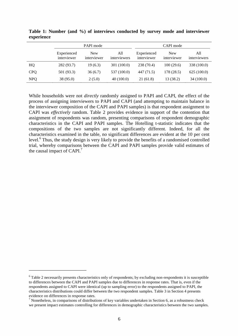
effects on telephone interviewing. Table 1 shows the quantity of HQs, CPQs and NPQs

completed by the mode used and the experience of the interviewer. Interviews conducted by

telephone have been excluded.5 We find that as a result of the greater concentration of new

interviewers assigned to CAPI, a greater proportion of interviews in this group were

completed by interviewers who were new to the HILDA Survey.

4 It was intended that if CAPI proved viable the HF would be fully integrated with the HQ and PQ. Indeed, this

is how it was implemented in Wave 9. 5 As we do not have a variable which records whether the HQ was completed by phone, we have classified an

HQ as being done by phone if all of the PQs completed on the same day as the HQ were by phone or if the HQ

was completed on a different day to the PQs and all of the PQs were completed by phone.

6

Table 1: Number (and %) of interviews conducted by survey mode and interviewer

experience

PAPI mode CAPI mode

Experienced

interviewer

New

interviewer

All

interviewers

Experienced

interviewer

New

interviewer

All

interviewers

HQ 282 (93.7) 19 (6.3) 301 (100.0) 238 (70.4) 100 (29.6) 338 (100.0)

CPQ 501 (93.3) 36 (6.7) 537 (100.0) 447 (71.5) 178 (28.5) 625 (100.0)

NPQ 38 (95.0) 2 (5.0) 40 (100.0) 21 (61.8) 13 (38.2) 34 (100.0)

While households were not directly randomly assigned to PAPI and CAPI, the effect of the

process of assigning interviewers to PAPI and CAPI (and attempting to maintain balance in

the interviewer composition of the CAPI and PAPI samples) is that respondent assignment to

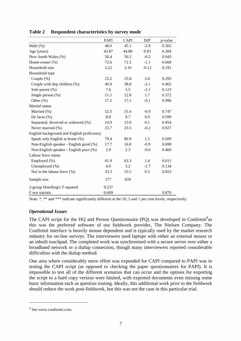
CAPI was effectively random. Table 2 provides evidence in support of the contention that

assignment of respondents was random, presenting comparisons of respondent demographic

characteristics in the CAPI and PAPI samples. The Hotelling t-statistic indicates that the

compositions of the two samples are not significantly different. Indeed, for all the

characteristics examined in the table, no significant differences are evident at the 10 per cent

level.6 Thus, the study design is very likely to provide the benefits of a randomised controlled

trial, whereby comparisons between the CAPI and PAPI samples provide valid estimates of

the causal impact of CAPI.7

6 Table 2 necessarily presents characteristics only of respondents; by excluding non-respondents it is susceptible

to differences between the CAPI and PAPI samples due to differences in response rates. That is, even if the

respondents assigned to CAPI were identical (up to sampling error) to the respondents assigned to PAPI, the

characteristics distributions could differ between the two respondent samples. Table 3 in Section 4 presents

evidence on differences in response rates. 7 Nonetheless, in comparisons of distributions of key variables undertaken in Section 6, as a robustness check

we present impact estimates controlling for differences in demographic characteristics between the two samples.

7

Table 2 Respondent characteristics by survey mode

PAPI CAPI Diff p-value

Male (%) 48.0 45.1 -2.9 0.302

Age (years) 43.87 44.80 0.93 0.384

New South Wales (%) 50.4 50.2 -0.2 0.943

Home-owner (%) 72.6 71.5 -1.1 0.668

Household size 3.22 3.10 -0.12 0.191

Household type

Couple (%) 23.2 25.8 2.6 0.295

Couple with dep children (%) 40.9 38.8 -2.1 0.462

Sole parent (%) 7.6 5.5 -2.1 0.123

Single person (%) 11.1 12.8 1.7 0.372

Other (%) 17.2 17.1 -0.1 0.996

Marital status

Married (%) 52.5 51.6 -0.9 0.747

De facto (%) 8.8 9.7 0.9 0.599

Separated, divorced or widowed (%) 14.9 15.0 0.1 0.954

Never married (%) 23.7 23.5 -0.2 0.927

English background and English proficiency

Speak only English at home (%) 79.4 80.9 1.5 0.509

Non-English speaker - English good (%) 17.7 16.8 -0.9 0.699

Non-English speaker - English poor (%) 2.9 2.3 -0.6 0.460

Labour force status

Employed (%) 61.9 63.3 1.4 0.611

Unemployed (%) 4.9 3.2 -1.7 0.134

Not in the labour force (%) 33.3 33.5 0.3 0.923

Sample size 577 659

2-group Hotelling's T-squared 9.237

F test statistic 0.609 0.870

Note: *, ** and *** indicate significantly different at the 10, 5 and 1 per cent levels, respectively.

Operational Issues

The CAPI script for the HQ and Person Questionnaire (PQ) was developed in Confirmit8as

this was the preferred software of our fieldwork provider, The Nielsen Company. The

Confirmit interface is heavily mouse dependent and is typically used by the market research

industry for on-line surveys. The interviewers used laptops with either an external mouse or

an inbuilt touchpad. The completed work was synchronised with a secure server over either a

broadband network or a dialup connection, though many interviewers reported considerable

difficulties with the dialup method.

One area where considerably more effort was expended for CAPI compared to PAPI was in

testing the CAPI script (as opposed to checking the paper questionnaires for PAPI). It is

impossible to test all of the different scenarios that can occur and the options for exporting

the script to a hard copy version were limited, with exported documents even missing some

basic information such as question routing. Ideally, this additional work prior to the fieldwork

should reduce the work post-fieldwork, but this was not the case in this particular trial.

8 See www.confirmit.com.

8

A final operational issue of note is that only limited use was made of dependent data in the

test. The variables we carried forward from the last interview were: sex, date of birth, date of

last interview, whether the respondent was employed at the last interview and the number of

employers they had. Obviously, the range of dependent data could be considerably extended,

as has been done in the BHPS after a detailed study of the effect (see Jäckle, 2008), and a

staged introduction of dependent data has been planned for the HILDA Survey.

4. Effects of CAPI on the response rates and interview situation

In this section, we consider the impact CAPI has had on the response rates, the respondents,

the interviewers, and the overall length of the interview. We cannot present any evidence

from this study about transcription errors as they cannot be detected without taking a

recording the actual interview and this was beyond the scope of our study.

Response Rates

Our analysis of the effect of CAPI on response rates is complicated by the fact that

interviewers were assigned to a particular mode rather than households: a household

originally approached by a CAPI interviewer may be followed up by a PAPI interviewer and

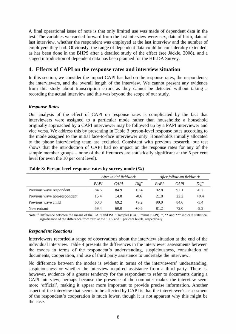
vice versa. We address this by presenting in Table 3 person-level response rates according to

the mode assigned to the initial face-to-face interviewer only. Households initially allocated

to the phone interviewing team are excluded. Consistent with previous research, our test

shows that the introduction of CAPI had no impact on the response rates for any of the

sample member groups – none of the differences are statistically significant at the 5 per cent

level (or even the 10 per cent level).

Table 3: Person-level response rates by survey mode (%)

After initial fieldwork After follow-up fieldwork

PAPI CAPI Diffa PAPI CAPI Diff

a

Previous wave respondent 84.6 84.9 +0.4 92.8 92.1 -0.7

Previous wave non-respondent 15.4 14.8 -0.6 21.8 22.2 +0.4

Previous wave child 60.0 69.2 +9.2 90.0 84.6 -5.4

New entrant 59.4 60.0 +0.6 81.2 72.0 -9.2

Note: a Difference between the means of the CAPI and PAPI samples (CAPI minus PAPI). *, ** and *** indicate statistical

significance of the difference from zero at the 10, 5 and 1 per cent levels, respectively.

Respondent Reactions

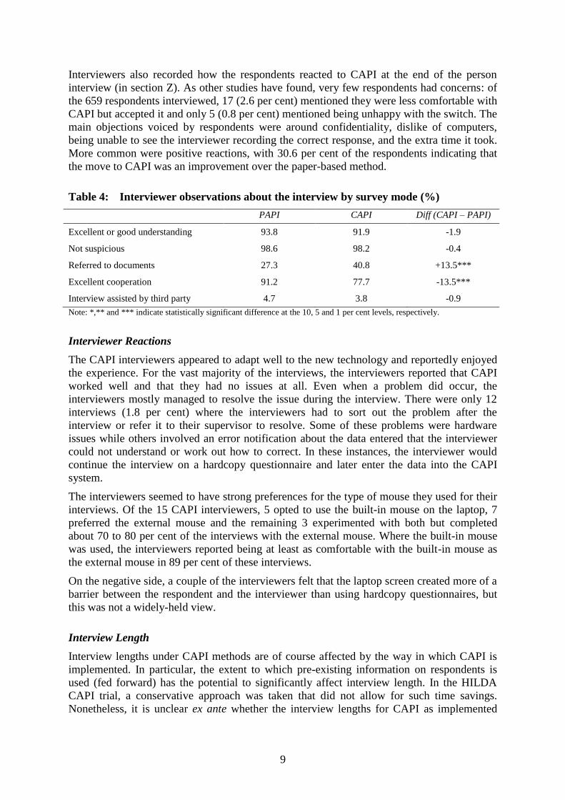
Interviewers recorded a range of observations about the interview situation at the end of the

individual interview. Table 4 presents the differences in the interviewer assessments between

the modes in terms of the respondent’s understanding, suspiciousness, consultation of

documents, cooperation, and use of third party assistance to undertake the interview.

No difference between the modes is evident in terms of the interviewers’ understanding,

suspiciousness or whether the interview required assistance from a third party. There is,

however, evidence of a greater tendency for the respondent to refer to documents during a

CAPI interview, perhaps because the presence of the computer makes the interview seem

more ‘official’, making it appear more important to provide precise information. Another

aspect of the interview that seems to be affected by CAPI is that the interviewer’s assessment

of the respondent’s cooperation is much lower, though it is not apparent why this might be

the case.

9

Interviewers also recorded how the respondents reacted to CAPI at the end of the person

interview (in section Z). As other studies have found, very few respondents had concerns: of

the 659 respondents interviewed, 17 (2.6 per cent) mentioned they were less comfortable with

CAPI but accepted it and only 5 (0.8 per cent) mentioned being unhappy with the switch. The

main objections voiced by respondents were around confidentiality, dislike of computers,

being unable to see the interviewer recording the correct response, and the extra time it took.

More common were positive reactions, with 30.6 per cent of the respondents indicating that

the move to CAPI was an improvement over the paper-based method.

Table 4: Interviewer observations about the interview by survey mode (%)

PAPI CAPI Diff (CAPI – PAPI)

Excellent or good understanding 93.8 91.9 -1.9

Not suspicious 98.6 98.2 -0.4

Referred to documents 27.3 40.8 +13.5***

Excellent cooperation 91.2 77.7 -13.5***

Interview assisted by third party 4.7 3.8 -0.9

Note: *,** and *** indicate statistically significant difference at the 10, 5 and 1 per cent levels, respectively.

Interviewer Reactions

The CAPI interviewers appeared to adapt well to the new technology and reportedly enjoyed

the experience. For the vast majority of the interviews, the interviewers reported that CAPI

worked well and that they had no issues at all. Even when a problem did occur, the

interviewers mostly managed to resolve the issue during the interview. There were only 12

interviews (1.8 per cent) where the interviewers had to sort out the problem after the

interview or refer it to their supervisor to resolve. Some of these problems were hardware

issues while others involved an error notification about the data entered that the interviewer

could not understand or work out how to correct. In these instances, the interviewer would

continue the interview on a hardcopy questionnaire and later enter the data into the CAPI

system.

The interviewers seemed to have strong preferences for the type of mouse they used for their

interviews. Of the 15 CAPI interviewers, 5 opted to use the built-in mouse on the laptop, 7

preferred the external mouse and the remaining 3 experimented with both but completed

about 70 to 80 per cent of the interviews with the external mouse. Where the built-in mouse

was used, the interviewers reported being at least as comfortable with the built-in mouse as

the external mouse in 89 per cent of these interviews.

On the negative side, a couple of the interviewers felt that the laptop screen created more of a

barrier between the respondent and the interviewer than using hardcopy questionnaires, but

this was not a widely-held view.

Interview Length

Interview lengths under CAPI methods are of course affected by the way in which CAPI is

implemented. In particular, the extent to which pre-existing information on respondents is

used (fed forward) has the potential to significantly affect interview length. In the HILDA

CAPI trial, a conservative approach was taken that did not allow for such time savings.

Nonetheless, it is unclear ex ante whether the interview lengths for CAPI as implemented

10

should be shorter or longer than PAPI. There are several factors contributing to shorter

interview lengths under CAPI, including:

1. Questionnaire routing is automated in CAPI.

2. Interviewers do not have to work out what text they should use for specific situations

(such as a child’s name, or text appropriate to people with two or more jobs) as this is

automatically generated in CAPI.

Balanced against this, however, are factors contributing to longer interview lengths in CAPI

than in PAPI:

1. Unusually high or inconsistent answers can be queried and resolved on the spot with

the respondent. This may result in the interviewer having to type in an explanation of

why the apparent difference is correct or they may have to work back through the

questionnaire to correct some previously entered data.

2. The CAPI system will not progress to the next question until the current question is

correctly filled in. (An error message is displayed whenever a response has not been

filled in or has been incorrectly filled in; e.g, a start date is entered but not an end

date, or the start date is after the end date.)

3. In PAPI, interviewers often read ahead and are asking the next question of the

respondent while they are finishing off filling in the answer to the last question. They

cannot do this in CAPI.

4. Many interviewers can write faster than they can type, though the effect of this will be

limited to the number of open-ended or partially-open response categories used.

5. There would be greater learning effects for the CAPI interviewers compared to PAPI.

Many of the interviewers were very experienced in the PAPI environment but none

had worked on a CAPI survey before.

Further, the interview lengths can be different due to different designs of the two systems –

how much use is made of data provided earlier in the interview or previous interviews, how

many questions are displayed on each screen and how questions in grids on the paper

questionnaire are programmed into CAPI.

It is not surprising, therefore, that previous studies have had mixed results regarding

interview length. It would depend on how each of these variables play out in the particular

combination employed by each study.

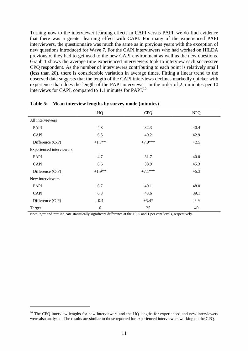
The average interview lengths recorded for both PAPI and CAPI in our Wave 7 test, based on

the recorded start and end times of the face-to-face interviews, are provided in Table 5.9 The

interview lengths for CAPI are longer than PAPI – the HQ is 35 per cent longer and the CPQ

is 24 per cent longer. These differences are more apparent amongst the experienced

interviewers than the new interviewers, perhaps because some of the ways the experienced

interviewers speed up the interview (such as reading ahead) are not possible in CAPI. It is

also likely that the mouse-dependent nature of Confirmit, when implemented in a laptop

environment, may have slowed the interview more than other CAPI software that could have

been used.

9 HQ and PQ times less than 1 minute or more than 90 minutes and PQ times less than 10 minutes or more than 90 minutes

were excluded, on the assumption that these case were due to problems with the timestamps.

11

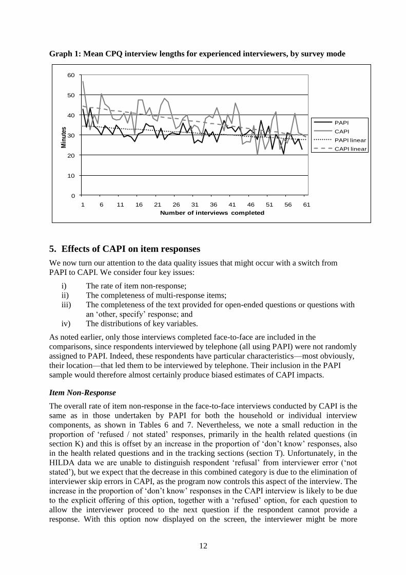
Turning now to the interviewer learning effects in CAPI versus PAPI, we do find evidence

that there was a greater learning effect with CAPI. For many of the experienced PAPI

interviewers, the questionnaire was much the same as in previous years with the exception of

new questions introduced for Wave 7. For the CAPI interviewers who had worked on HILDA

previously, they had to get used to the new CAPI environment as well as the new questions.

Graph 1 shows the average time experienced interviewers took to interview each successive

CPQ respondent. As the number of interviewers contributing to each point is relatively small

(less than 20), there is considerable variation in average times. Fitting a linear trend to the

observed data suggests that the length of the CAPI interviews declines markedly quicker with

experience than does the length of the PAPI interviews—in the order of 2.5 minutes per 10

interviews for CAPI, compared to 1.1 minutes for PAPI.10

Table 5: Mean interview lengths by survey mode (minutes)

HQ CPQ NPQ

All interviewers

PAPI 4.8 32.3 40.4

CAPI 6.5 40.2 42.9

Difference (C-P) +1.7** +7.9*** +2.5

Experienced interviewers

PAPI 4.7 31.7 40.0

CAPI 6.6 38.9 45.3

Difference (C-P) +1.9** +7.1*** +5.3

New interviewers

PAPI 6.7 40.1 48.0

CAPI 6.3 43.6 39.1

Difference (C-P) -0.4 +3.4* -8.9

Target 6 35 40


10

The CPQ interview lengths for new interviewers and the HQ lengths for experienced and new interviewers

were also analysed. The results are similar to those reported for experienced interviewers working on the CPQ.

12

Graph 1: Mean CPQ interview lengths for experienced interviewers, by survey mode

0

10

20

30

40

50

60

1 6 11 16 21 26 31 36 41 46 51 56 61

Min

ute

s

Number of interviews completed

PAPI

CAPI

PAPI linear

CAPI linear

5. Effects of CAPI on item responses

We now turn our attention to the data quality issues that might occur with a switch from

PAPI to CAPI. We consider four key issues:

i) The rate of item non-response;

ii) The completeness of multi-response items;

iii) The completeness of the text provided for open-ended questions or questions with

an ‘other, specify’ response; and

iv) The distributions of key variables.

As noted earlier, only those interviews completed face-to-face are included in the

comparisons, since respondents interviewed by telephone (all using PAPI) were not randomly

assigned to PAPI. Indeed, these respondents have particular characteristics—most obviously,

their location—that led them to be interviewed by telephone. Their inclusion in the PAPI

sample would therefore almost certainly produce biased estimates of CAPI impacts.

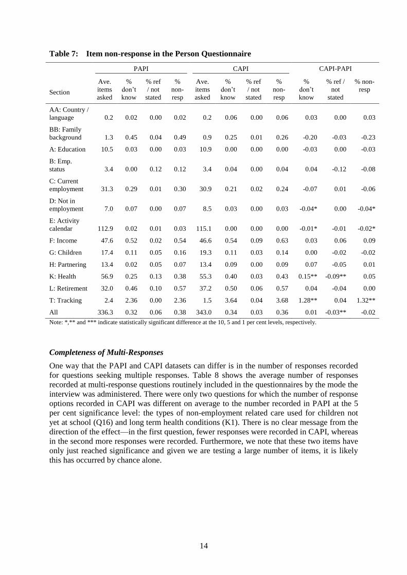
Item Non-Response

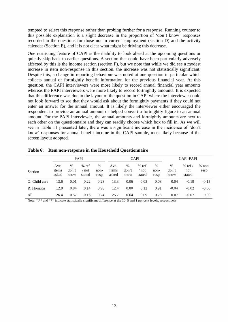
The overall rate of item non-response in the face-to-face interviews conducted by CAPI is the

same as in those undertaken by PAPI for both the household or individual interview

components, as shown in Tables 6 and 7. Nevertheless, we note a small reduction in the

proportion of ‘refused / not stated’ responses, primarily in the health related questions (in

section K) and this is offset by an increase in the proportion of ‘don’t know’ responses, also

in the health related questions and in the tracking sections (section T). Unfortunately, in the

HILDA data we are unable to distinguish respondent ‘refusal’ from interviewer error (‘not

stated’), but we expect that the decrease in this combined category is due to the elimination of

interviewer skip errors in CAPI, as the program now controls this aspect of the interview. The

increase in the proportion of ‘don’t know’ responses in the CAPI interview is likely to be due

to the explicit offering of this option, together with a ‘refused’ option, for each question to

allow the interviewer proceed to the next question if the respondent cannot provide a

response. With this option now displayed on the screen, the interviewer might be more

13

tempted to select this response rather than probing further for a response. Running counter to

this possible explanation is a slight decrease in the proportion of ‘don’t know’ responses

recorded in the questions for those not in current employment (section D) and the activity

calendar (Section E), and it is not clear what might be driving this decrease.

One restricting feature of CAPI is the inability to look ahead at the upcoming questions or

quickly skip back to earlier questions. A section that could have been particularly adversely

affected by this is the income section (section F), but we note that while we did see a modest

increase in item non-response in this section, the increase was not statistically significant.

Despite this, a change in reporting behaviour was noted at one question in particular which

collects annual or fortnightly benefit information for the previous financial year. At this

question, the CAPI interviewers were more likely to record annual financial year amounts

whereas the PAPI interviewers were more likely to record fortnightly amounts. It is expected

that this difference was due to the layout of the question in CAPI where the interviewer could

not look forward to see that they would ask about the fortnightly payments if they could not

enter an answer for the annual amount. It is likely the interviewer either encouraged the

respondent to provide an annual amount or helped convert a fortnightly figure to an annual

amount. For the PAPI interviewer, the annual amounts and fortnightly amounts are next to

each other on the questionnaire and they can readily choose which box to fill in. As we will

see in Table 11 presented later, there was a significant increase in the incidence of ‘don’t

know’ responses for annual benefit income in the CAPI sample, most likely because of the

screen layout adopted.

Table 6: Item non-response in the Household Questionnaire

Section

PAPI CAPI CAPI-PAPI

Ave.

items

asked

%

don’t

know

% ref

/ not

stated

%

non-

resp

Ave.

items

asked

%

don’t

know

% ref

/ not

stated

%

non-

resp

%

don’t

know

% ref /

not

stated

% non-

resp

Q: Child care 13.6 0.01 0.22 0.23 13.3 0.06 0.03 0.08 0.04 -0.19 -0.15

R: Housing 12.8 0.84 0.14 0.98 12.4 0.80 0.12 0.91 -0.04 -0.02 -0.06

All 26.4 0.57 0.16 0.74 25.7 0.64 0.09 0.73 0.07 -0.07 0.00


14

Table 7: Item non-response in the Person Questionnaire

Section

PAPI CAPI CAPI-PAPI

Ave.

items

asked

%

don’t

know

% ref

/ not

stated

%

non-

resp

Ave.

items

asked

%

don’t

know

% ref

/ not

stated

%

non-

resp

%

don’t

know

% ref /

not

stated

% non-

resp

AA: Country /

language 0.2 0.02 0.00 0.02 0.2 0.06 0.00 0.06 0.03 0.00 0.03

BB: Family

background 1.3 0.45 0.04 0.49 0.9 0.25 0.01 0.26 -0.20 -0.03 -0.23

A: Education 10.5 0.03 0.00 0.03 10.9 0.00 0.00 0.00 -0.03 0.00 -0.03

B: Emp.

status 3.4 0.00 0.12 0.12 3.4 0.04 0.00 0.04 0.04 -0.12 -0.08

C: Current

employment 31.3 0.29 0.01 0.30 30.9 0.21 0.02 0.24 -0.07 0.01 -0.06

D: Not in

employment 7.0 0.07 0.00 0.07 8.5 0.03 0.00 0.03 -0.04* 0.00 -0.04*

E: Activity

calendar 112.9 0.02 0.01 0.03 115.1 0.00 0.00 0.00 -0.01* -0.01 -0.02*

F: Income 47.6 0.52 0.02 0.54 46.6 0.54 0.09 0.63 0.03 0.06 0.09

G: Children 17.4 0.11 0.05 0.16 19.3 0.11 0.03 0.14 0.00 -0.02 -0.02

H: Partnering 13.4 0.02 0.05 0.07 13.4 0.09 0.00 0.09 0.07 -0.05 0.01

K: Health 56.9 0.25 0.13 0.38 55.3 0.40 0.03 0.43 0.15** -0.09** 0.05

L: Retirement 32.0 0.46 0.10 0.57 37.2 0.50 0.06 0.57 0.04 -0.04 0.00

T: Tracking 2.4 2.36 0.00 2.36 1.5 3.64 0.04 3.68 1.28** 0.04 1.32**

All 336.3 0.32 0.06 0.38 343.0 0.34 0.03 0.36 0.01 -0.03** -0.02


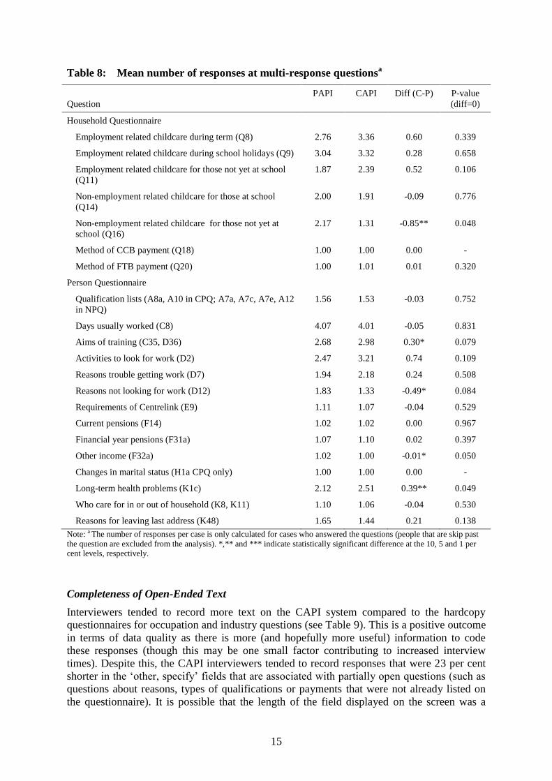
Completeness of Multi-Responses

One way that the PAPI and CAPI datasets can differ is in the number of responses recorded

for questions seeking multiple responses. Table 8 shows the average number of responses

recorded at multi-response questions routinely included in the questionnaires by the mode the

interview was administered. There were only two questions for which the number of response

options recorded in CAPI was different on average to the number recorded in PAPI at the 5

per cent significance level: the types of non-employment related care used for children not

yet at school (Q16) and long term health conditions (K1). There is no clear message from the

direction of the effect—in the first question, fewer responses were recorded in CAPI, whereas

in the second more responses were recorded. Furthermore, we note that these two items have

only just reached significance and given we are testing a large number of items, it is likely

this has occurred by chance alone.

15

Table 8: Mean number of responses at multi-response questionsa

Question

PAPI CAPI Diff (C-P) P-value

(diff=0)

Household Questionnaire

Employment related childcare during term (Q8) 2.76 3.36 0.60 0.339

Employment related childcare during school holidays (Q9) 3.04 3.32 0.28 0.658

Employment related childcare for those not yet at school

(Q11)

1.87 2.39 0.52 0.106

Non-employment related childcare for those at school

(Q14)

2.00 1.91 -0.09 0.776

Non-employment related childcare for those not yet at

school (Q16)

2.17 1.31 -0.85** 0.048

Method of CCB payment (Q18) 1.00 1.00 0.00 -

Method of FTB payment (Q20) 1.00 1.01 0.01 0.320

Person Questionnaire

Qualification lists (A8a, A10 in CPQ; A7a, A7c, A7e, A12

in NPQ)

1.56 1.53 -0.03 0.752

Days usually worked (C8) 4.07 4.01 -0.05 0.831

Aims of training (C35, D36) 2.68 2.98 0.30* 0.079

Activities to look for work (D2) 2.47 3.21 0.74 0.109

Reasons trouble getting work (D7) 1.94 2.18 0.24 0.508

Reasons not looking for work (D12) 1.83 1.33 -0.49* 0.084

Requirements of Centrelink (E9) 1.11 1.07 -0.04 0.529

Current pensions (F14) 1.02 1.02 0.00 0.967

Financial year pensions (F31a) 1.07 1.10 0.02 0.397

Other income (F32a) 1.02 1.00 -0.01* 0.050

Changes in marital status (H1a CPQ only) 1.00 1.00 0.00 -

Long-term health problems (K1c) 2.12 2.51 0.39** 0.049

Who care for in or out of household (K8, K11) 1.10 1.06 -0.04 0.530

Reasons for leaving last address (K48) 1.65 1.44 0.21 0.138

Note: a The number of responses per case is only calculated for cases who answered the questions (people that are skip past

the question are excluded from the analysis). *,** and *** indicate statistically significant difference at the 10, 5 and 1 per

cent levels, respectively.

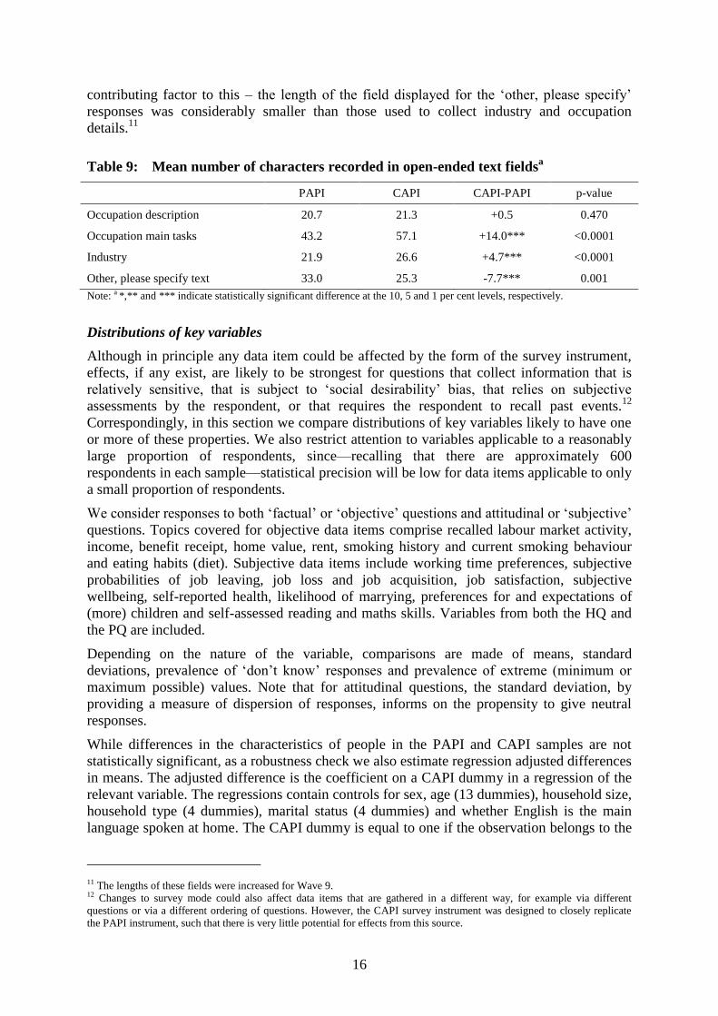
Completeness of Open-Ended Text

Interviewers tended to record more text on the CAPI system compared to the hardcopy

questionnaires for occupation and industry questions (see Table 9). This is a positive outcome

in terms of data quality as there is more (and hopefully more useful) information to code

these responses (though this may be one small factor contributing to increased interview

times). Despite this, the CAPI interviewers tended to record responses that were 23 per cent

shorter in the ‘other, specify’ fields that are associated with partially open questions (such as

questions about reasons, types of qualifications or payments that were not already listed on

the questionnaire). It is possible that the length of the field displayed on the screen was a

16

contributing factor to this – the length of the field displayed for the ‘other, please specify’

responses was considerably smaller than those used to collect industry and occupation

details.11

Table 9: Mean number of characters recorded in open-ended text fieldsa

PAPI CAPI CAPI-PAPI p-value

Occupation description 20.7 21.3 +0.5 0.470

Occupation main tasks 43.2 57.1 +14.0*** <0.0001

Industry 21.9 26.6 +4.7*** <0.0001

Other, please specify text 33.0 25.3 -7.7*** 0.001

Note: a *,** and *** indicate statistically significant difference at the 10, 5 and 1 per cent levels, respectively.

Distributions of key variables

Although in principle any data item could be affected by the form of the survey instrument,

effects, if any exist, are likely to be strongest for questions that collect information that is

relatively sensitive, that is subject to ‘social desirability’ bias, that relies on subjective

assessments by the respondent, or that requires the respondent to recall past events.12

Correspondingly, in this section we compare distributions of key variables likely to have one

or more of these properties. We also restrict attention to variables applicable to a reasonably

large proportion of respondents, since—recalling that there are approximately 600

respondents in each sample—statistical precision will be low for data items applicable to only

a small proportion of respondents.

We consider responses to both ‘factual’ or ‘objective’ questions and attitudinal or ‘subjective’

questions. Topics covered for objective data items comprise recalled labour market activity,

income, benefit receipt, home value, rent, smoking history and current smoking behaviour

and eating habits (diet). Subjective data items include working time preferences, subjective

probabilities of job leaving, job loss and job acquisition, job satisfaction, subjective

wellbeing, self-reported health, likelihood of marrying, preferences for and expectations of

(more) children and self-assessed reading and maths skills. Variables from both the HQ and

the PQ are included.

Depending on the nature of the variable, comparisons are made of means, standard

deviations, prevalence of ‘don’t know’ responses and prevalence of extreme (minimum or

maximum possible) values. Note that for attitudinal questions, the standard deviation, by

providing a measure of dispersion of responses, informs on the propensity to give neutral

responses.

While differences in the characteristics of people in the PAPI and CAPI samples are not

statistically significant, as a robustness check we also estimate regression adjusted differences

in means. The adjusted difference is the coefficient on a CAPI dummy in a regression of the

relevant variable. The regressions contain controls for sex, age (13 dummies), household size,

household type (4 dummies), marital status (4 dummies) and whether English is the main

language spoken at home. The CAPI dummy is equal to one if the observation belongs to the

11 The lengths of these fields were increased for Wave 9. 12 Changes to survey mode could also affect data items that are gathered in a different way, for example via different

questions or via a different ordering of questions. However, the CAPI survey instrument was designed to closely replicate

the PAPI instrument, such that there is very little potential for effects from this source.

17

CAPI sample and zero if the observation belongs to the PAPI sample. The coefficient

provides an estimate of the difference in means controlling for differences in the sex, age,

household size and type, marital status and language spoken composition of the two samples.

For each distributional comparison, we exclude observations with ‘missing’ values (due to

non-response or non-applicability of the data item), although note that ‘don’t know’ is treated

as a valid response (and therefore not missing). For continuous financial variables, we also

exclude observations with top-coded values.

Objective data

Table 10 compares means and standard deviations of various labour market-related variables

that require the respondent to recall past events. While there is some potential for sensitivity

and social desirability bias, for example in relationship to unemployment experience and

leave taken, the most likely source of difference between PAPI and CAPI responses is

differences in the way past events are recalled. The top two panels of Table 10 are derived

from responses to the employment and education calendar, which requires respondents to

report on labour market and education activity in each third of each month since the

beginning of the previous year. The variables reported in the table relate to the 2006 calendar

year. No significant differences in means or standard deviations are evident for the

percentage of time spent in each labour force state, but there is a difference in the mean

reported number of jobs of 0.07, which is significant at the 10 per cent level in the case of the

raw difference and significant at the 5 per cent level in the case of the regression-adjusted

difference. The mean number is higher for CAPI, but it is not clear whether this translates to

more or less recall bias.

The second panel presents comparisons for reported number of days of each of three types of

leave taken in the 12 months leading up to the interview. PAPI and CAPI means are not

significantly different, but it appears that dispersion in reports of unpaid leave taken is greater

for the CAPI mode. The bottom panel compares total length of tenure in current job and in

current occupation. In both cases, the estimated mean is not significantly different between

the two survey modes, but the standard deviation is significantly greater for CAPI. Greater

dispersion in reported tenure might reflect more accurate reporting, or simply greater random

variation (noise).

18

Table 10: Distributions of variables for recalled labour market activity

Mean Standard deviation

PAPI CAPI Diff a

p-valueb

Adj diff a

p-valueb

PAPI CAPI Ratioc

p-valued

No. of jobs last year 0.79 0.86 0.07 0.084* 0.07 0.050** 0.66 0.74 1.12 0.247

Percentage of last year…

…employed 61.6 61.9 0.3 0.919 -0.1 0.954 46.9 46.2 0.99 0.213

…unemployed 3.4 4.2 0.8 0.393 0.9 0.341 15.2 16.3 1.07 0.134

…not in the labour force 35.0 33.9 -1.0 0.692 -0.7 0.726 46.1 45.9 1.00 0.497

Annual leave taken (days) 8.5 8.8 0.3 0.758 0.1 0.579 12.4 12.2 0.98 0.777

Sick leave taken (days) 2.1 2.3 0.3 0.454 0.2 0.641 5.7 4.9 0.86 0.330

Unpaid leave taken (days) 1.2 2.4 1.2 0.103 1.0 0.161 4.6 13.5 2.93*** 0.002

Job tenure (years) 6.6 7.0 0.4 0.477 0.0 0.934 7.6 8.7 1.14** 0.045

Occupation tenure (years) 8.8 9.8 1.0 0.169 0.6 0.347 10.0 10.6 1.06* 0.053

Notes: a. Difference between the means of the CAPI and PAPI samples (CAPI minus PAPI). *, **, *** indicated

statistical significance of the difference from zero at the 10, 5 and 1 per cent levels, respectively.

b. p-value is the significance level of the difference in the means from zero.

c. Ratio of the CAPI standard deviation to the PAPI standard deviation. *, **, *** indicate the ratio of the

standard deviations is significantly different from one at the 10, 5 and 1 per cent levels, respectively, based on

Levene's (1960) statistic.

d. p-value is the significance level of the difference of the ratio of the standard deviations from one.

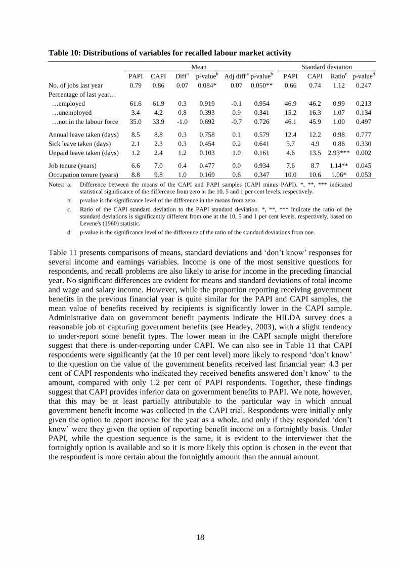
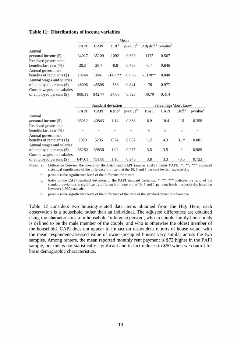
Table 11 presents comparisons of means, standard deviations and ‘don’t know’ responses for

several income and earnings variables. Income is one of the most sensitive questions for

respondents, and recall problems are also likely to arise for income in the preceding financial

year. No significant differences are evident for means and standard deviations of total income

and wage and salary income. However, while the proportion reporting receiving government

benefits in the previous financial year is quite similar for the PAPI and CAPI samples, the

mean value of benefits received by recipients is significantly lower in the CAPI sample.

Administrative data on government benefit payments indicate the HILDA survey does a

reasonable job of capturing government benefits (see Headey, 2003), with a slight tendency

to under-report some benefit types. The lower mean in the CAPI sample might therefore

suggest that there is under-reporting under CAPI. We can also see in Table 11 that CAPI

respondents were significantly (at the 10 per cent level) more likely to respond ‘don’t know’

to the question on the value of the government benefits received last financial year: 4.3 per

cent of CAPI respondents who indicated they received benefits answered don’t know’ to the

amount, compared with only 1.2 per cent of PAPI respondents. Together, these findings

suggest that CAPI provides inferior data on government benefits to PAPI. We note, however,

that this may be at least partially attributable to the particular way in which annual

government benefit income was collected in the CAPI trial. Respondents were initially only

given the option to report income for the year as a whole, and only if they responded ‘don’t

know’ were they given the option of reporting benefit income on a fortnightly basis. Under

PAPI, while the question sequence is the same, it is evident to the interviewer that the

fortnightly option is available and so it is more likely this option is chosen in the event that

the respondent is more certain about the fortnightly amount than the annual amount.

19

Table 11: Distributions of income variables

Mean

PAPI CAPI Diff a

p-valueb

Adj diff a

p-valueb

Annual

personal income ($) 34017 35109 1092 0.639 1175 0.567

Received government

benefits last year (%) 29.5 28.7 -0.8 0.763 -0.4 0.846

Annual government

benefits of recipients ($) 10244 8841 -1403** 0.036 -1370** 0.040

Annual wages and salaries

of employed persons ($) 46096 45508 -588 0.841 -76 0.977

Current wages and salaries

of employed persons ($) 908.11 942.77 34.66 0.528 40.79 0.414

Standard deviation Percentage 'don't know'

PAPI CAPI Ratioc

p-valued

PAPI CAPI Diff a

p-valueb

Annual

personal income ($) 35912 40843 1.14 0.386 8.9 10.4 1.5 0.358

Received government

benefits last year (%) - - - - 0 0 0 -

Annual government

benefits of recipients ($) 7020 5205 0.74 0.657 1.2 4.3 3.1* 0.081

Annual wages and salaries

of employed persons ($) 38260 39836 1.04 0.975 3.5 3.5 0 0.989

Current wages and salaries

of employed persons ($) 647.01 751.98 1.16 0.246 3.8 3.3 -0.5 0.722



b. p-value is the significance level of the difference from zero.





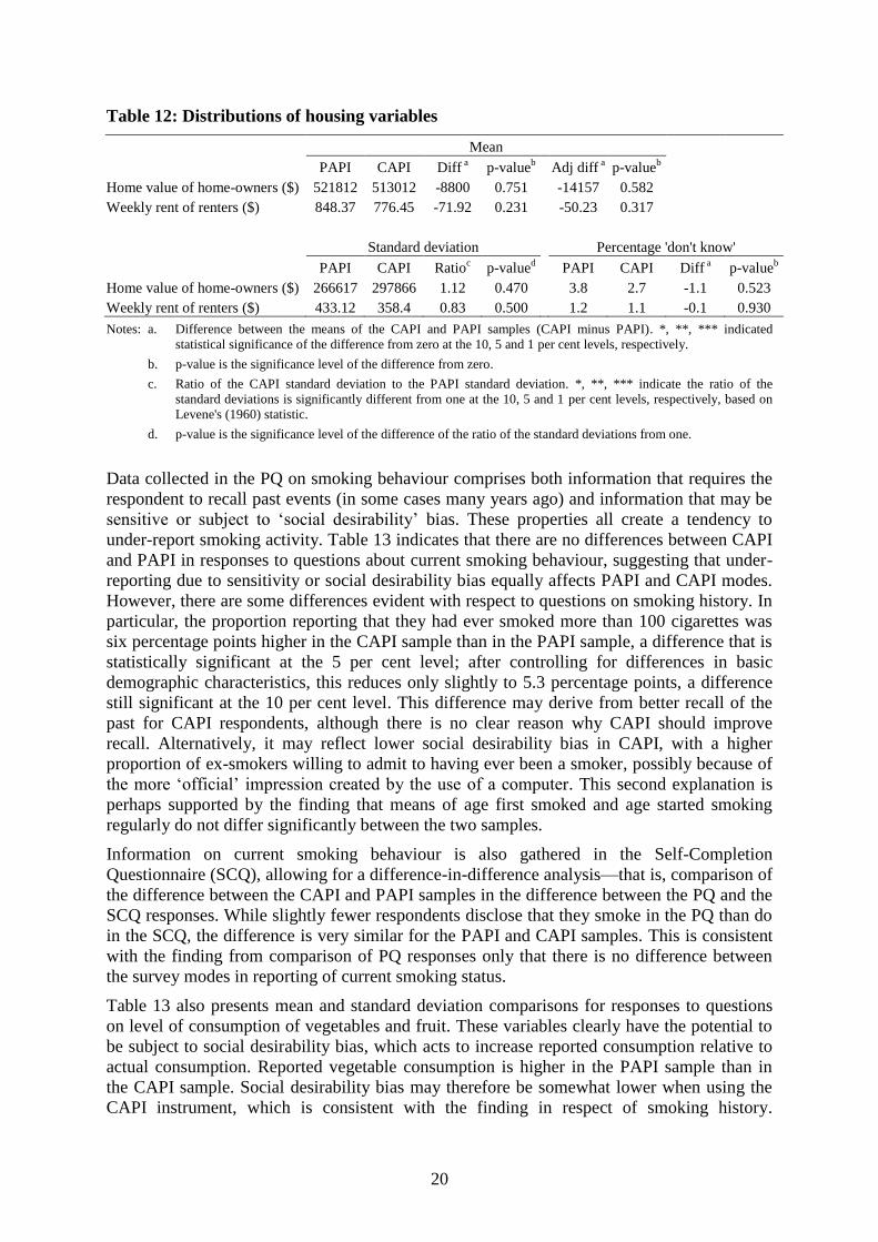
Table 12 considers two housing-related data items obtained from the HQ. Here, each

observation is a household rather than an individual. The adjusted differences are obtained

using the characteristics of a household ‘reference person’, who in couple-family households

is defined to be the male member of the couple, and who is otherwise the oldest member of

the household. CAPI does not appear to impact on respondent reports of house value, with

the mean respondent-assessed value of owner-occupied houses very similar across the two

samples. Among renters, the mean reported monthly rent payment is $72 higher in the PAPI

sample, but this is not statistically significant and in fact reduces to $50 when we control for

basic demographic characteristics.

20

Table 12: Distributions of housing variables

Mean

PAPI CAPI Diff a

p-valueb

Adj diff a

p-valueb

Home value of home-owners ($) 521812 513012 -8800 0.751 -14157 0.582

Weekly rent of renters ($) 848.37 776.45 -71.92 0.231 -50.23 0.317

Standard deviation Percentage 'don't know'

PAPI CAPI Ratioc

p-valued

PAPI CAPI Diff a

p-valueb

Home value of home-owners ($) 266617 297866 1.12 0.470 3.8 2.7 -1.1 0.523

Weekly rent of renters ($) 433.12 358.4 0.83 0.500 1.2 1.1 -0.1 0.930








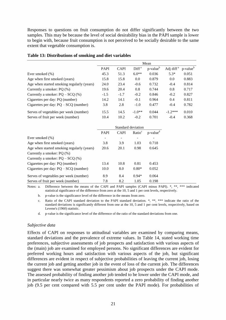
Data collected in the PQ on smoking behaviour comprises both information that requires the

respondent to recall past events (in some cases many years ago) and information that may be

sensitive or subject to ‘social desirability’ bias. These properties all create a tendency to

under-report smoking activity. Table 13 indicates that there are no differences between CAPI

and PAPI in responses to questions about current smoking behaviour, suggesting that under-

reporting due to sensitivity or social desirability bias equally affects PAPI and CAPI modes.

However, there are some differences evident with respect to questions on smoking history. In

particular, the proportion reporting that they had ever smoked more than 100 cigarettes was

six percentage points higher in the CAPI sample than in the PAPI sample, a difference that is

statistically significant at the 5 per cent level; after controlling for differences in basic

demographic characteristics, this reduces only slightly to 5.3 percentage points, a difference

still significant at the 10 per cent level. This difference may derive from better recall of the

past for CAPI respondents, although there is no clear reason why CAPI should improve

recall. Alternatively, it may reflect lower social desirability bias in CAPI, with a higher

proportion of ex-smokers willing to admit to having ever been a smoker, possibly because of

the more ‘official’ impression created by the use of a computer. This second explanation is

perhaps supported by the finding that means of age first smoked and age started smoking

regularly do not differ significantly between the two samples.

Information on current smoking behaviour is also gathered in the Self-Completion

Questionnaire (SCQ), allowing for a difference-in-difference analysis—that is, comparison of

the difference between the CAPI and PAPI samples in the difference between the PQ and the

SCQ responses. While slightly fewer respondents disclose that they smoke in the PQ than do

in the SCQ, the difference is very similar for the PAPI and CAPI samples. This is consistent

with the finding from comparison of PQ responses only that there is no difference between

the survey modes in reporting of current smoking status.

Table 13 also presents mean and standard deviation comparisons for responses to questions

on level of consumption of vegetables and fruit. These variables clearly have the potential to

be subject to social desirability bias, which acts to increase reported consumption relative to

actual consumption. Reported vegetable consumption is higher in the PAPI sample than in

the CAPI sample. Social desirability bias may therefore be somewhat lower when using the

CAPI instrument, which is consistent with the finding in respect of smoking history.

21

Responses to questions on fruit consumption do not differ significantly between the two

samples. This may be because the level of social desirability bias in the PAPI sample is lower

to begin with, because fruit consumption is not perceived to be socially desirable to the same

extent that vegetable consumption is.

Table 13: Distributions of smoking and diet variables

Mean

PAPI CAPI Diff a

p-valueb

Adj diff a

p-valueb

Ever smoked (%) 45.3 51.3 6.0** 0.036 5.3* 0.051

Age when first smoked (years) 15.8 15.8 0.0 0.879 0.0 0.883

Age when started smoking regularly (years) 24.0 23.4 -0.6 0.732 -0.4 0.814

Currently a smoker: PQ (%) 19.6 20.4 0.8 0.744 0.8 0.717

Currently a smoker: PQ – SCQ (%) -1.5 -1.7 -0.2 0.846 -0.2 0.827

Cigarettes per day: PQ (number) 14.2 14.1 -0.1 0.964 0.4 0.811

Cigarettes per day: PQ – SCQ (number) 3.8 2.8 -1.0 0.477 -0.4 0.782

Serves of vegetables per week (number) 15.5 14.5 -1.0** 0.044 -1.2*** 0.010

Serves of fruit per week (number) 10.4 10.2 -0.2 0.701 -0.4 0.368

Standard deviation

PAPI CAPI Ratioc

p-valued

Ever smoked (%) - - - -

Age when first smoked (years) 3.8 3.9 1.03 0.718

Age when started smoking regularly (years) 20.6 20.1 0.98 0.645

Currently a smoker: PQ (%)

Currently a smoker: PQ – SCQ (%)

Cigarettes per day: PQ (number) 13.4 10.8 0.81 0.453

Cigarettes per day: PQ – SCQ (number) 10.0 8.0 0.80* 0.052

Serves of vegetables per week (number) 8.9 8.4 0.94* 0.064

Serves of fruit per week (number) 7.8 8.2 1.05 0.198



b. p-value is the significance level of the difference in the means from zero.





Subjective data

Effects of CAPI on responses to attitudinal variables are examined by comparing means,

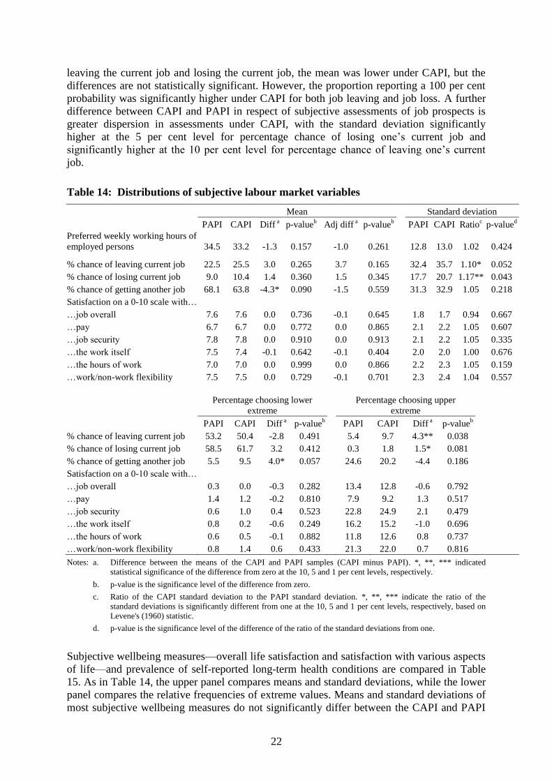
standard deviations and the prevalence of extreme values. In Table 14, stated working time

preferences, subjective assessments of job prospects and satisfaction with various aspects of

the (main) job are examined for employed persons. No significant differences are evident for

preferred working hours and satisfaction with various aspects of the job, but significant

differences are evident in respect of subjective probabilities of leaving the current job, losing

the current job and getting another job in the event of loss of the current job. The differences

suggest there was somewhat greater pessimism about job prospects under the CAPI mode.

The assessed probability of finding another job tended to be lower under the CAPI mode, and

in particular nearly twice as many respondents reported a zero probability of finding another

job (9.5 per cent compared with 5.5 per cent under the PAPI mode). For probabilities of

22

leaving the current job and losing the current job, the mean was lower under CAPI, but the

differences are not statistically significant. However, the proportion reporting a 100 per cent

probability was significantly higher under CAPI for both job leaving and job loss. A further

difference between CAPI and PAPI in respect of subjective assessments of job prospects is

greater dispersion in assessments under CAPI, with the standard deviation significantly

higher at the 5 per cent level for percentage chance of losing one’s current job and

significantly higher at the 10 per cent level for percentage chance of leaving one’s current

job.

Table 14: Distributions of subjective labour market variables


PAPI CAPI Diff a

p-valueb

Adj diff a

p-valueb

PAPI CAPI Ratioc

p-valued

Preferred weekly working hours of

employed persons 34.5 33.2 -1.3 0.157 -1.0 0.261 12.8 13.0 1.02 0.424

% chance of leaving current job 22.5 25.5 3.0 0.265 3.7 0.165 32.4 35.7 1.10* 0.052

% chance of losing current job 9.0 10.4 1.4 0.360 1.5 0.345 17.7 20.7 1.17** 0.043

% chance of getting another job 68.1 63.8 -4.3* 0.090 -1.5 0.559 31.3 32.9 1.05 0.218

Satisfaction on a 0-10 scale with…

…job overall 7.6 7.6 0.0 0.736 -0.1 0.645 1.8 1.7 0.94 0.667

…pay 6.7 6.7 0.0 0.772 0.0 0.865 2.1 2.2 1.05 0.607

…job security 7.8 7.8 0.0 0.910 0.0 0.913 2.1 2.2 1.05 0.335

…the work itself 7.5 7.4 -0.1 0.642 -0.1 0.404 2.0 2.0 1.00 0.676

…the hours of work 7.0 7.0 0.0 0.999 0.0 0.866 2.2 2.3 1.05 0.159

…work/non-work flexibility 7.5 7.5 0.0 0.729 -0.1 0.701 2.3 2.4 1.04 0.557

Percentage choosing lower

extreme

Percentage choosing upper

extreme

PAPI CAPI Diff a

p-valueb

PAPI CAPI Diff a

p-valueb

% chance of leaving current job 53.2 50.4 -2.8 0.491 5.4 9.7 4.3** 0.038

% chance of losing current job 58.5 61.7 3.2 0.412 0.3 1.8 1.5* 0.081

% chance of getting another job 5.5 9.5 4.0* 0.057 24.6 20.2 -4.4 0.186


…job overall 0.3 0.0 -0.3 0.282 13.4 12.8 -0.6 0.792

…pay 1.4 1.2 -0.2 0.810 7.9 9.2 1.3 0.517

…job security 0.6 1.0 0.4 0.523 22.8 24.9 2.1 0.479

…the work itself 0.8 0.2 -0.6 0.249 16.2 15.2 -1.0 0.696

…the hours of work 0.6 0.5 -0.1 0.882 11.8 12.6 0.8 0.737

…work/non-work flexibility 0.8 1.4 0.6 0.433 21.3 22.0 0.7 0.816








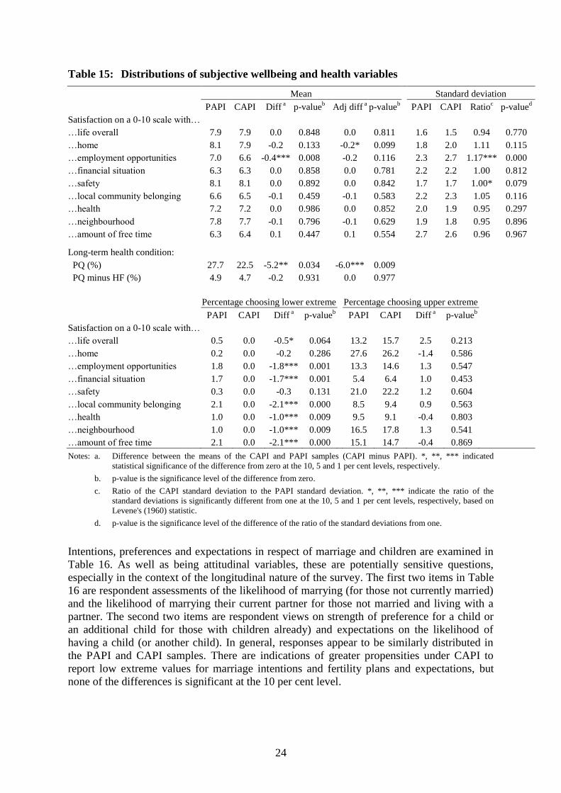
Subjective wellbeing measures—overall life satisfaction and satisfaction with various aspects

of life—and prevalence of self-reported long-term health conditions are compared in Table

15. As in Table 14, the upper panel compares means and standard deviations, while the lower

panel compares the relative frequencies of extreme values. Means and standard deviations of

most subjective wellbeing measures do not significantly differ between the CAPI and PAPI

23

samples. The notable exception is that mean satisfaction with employment opportunities is

substantially lower in the CAPI sample, and the standard deviation for this variable is

considerably higher in the CAPI sample. This may suggest less propensity to give a neutral

response to this question, with this decrease in neutrality more often leading to a more

negative assessment than a more positive assessment.

The results on percentages reporting extreme values show that no respondent in the CAPI

sample selected the lowest value for satisfaction (complete dissatisfaction) with any aspect of

life—including employment opportunities. Percentages choosing this option in the PAPI

sample were also low, but in all cases exceeded zero and in fact were in all but two cases

significantly different from the CAPI sample. There is thus some indication of lower

propensity to report (low) extreme values under CAPI, although it is curious that this is not

found in relation to job satisfaction of employees (Table 14).

Information on the presence of a long-term health condition is available for each respondent

from both the HF and the PQ. PAPI-CAPI comparisons of the proportion of respondents with

a long-term health condition are presented for the PQ variable. The proportion reporting a

condition is 5.2 percentage points higher in the PAPI sample, a difference which is significant

at the 5 per cent level. Controlling for differences in basic demographic characteristics, the

difference increases to 6 percentage points, which is significant at the 1 per cent level. One

interpretation of this CAPI-PAPI difference in PQ responses is that there is a slightly lower

propensity to report long-term health conditions when the survey is CAPI administered. For

example, it may be that the presence of a computer creates a greater sense of formality or that

the survey is somehow more ‘official’, causing respondents to be less likely to report less-

serious health conditions.

Another interpretation of the difference in the PQ measure of the presence of a long-term

health condition is that the CAPI and PAPI samples genuinely have different proportions

with long-term health conditions. We can investigate this interpretation by drawing on the HF

measure of the presence of a long-term health condition in a similar manner as was done with

smoking status using the SCQ. Specifically, using the fact that the HF was administered by

PAPI methods in both the PAPI and CAPI samples, we can examine whether the difference

between the HF and PQ measure is different for the PAPI and CAPI samples. Thus, Table 15

presents this ‘difference-in-difference’. As might be expected, in both samples the proportion

of respondents classified as having a long-term health condition is higher when the PQ is

used, since the HF information is gathered for all household members from only one member

of the household. However, the raw difference-in-difference estimate of 0.2 is not

significantly different from zero, while the regression-adjusted difference-in-difference

estimate is zero. That is, the difference between the HF and the PQ is essentially the same for

the PAPI and CAPI samples.

The HF-PQ difference-in-difference finding supports the contention that the CAPI sample

does genuinely have a lower incidence of long-term health conditions. However, a counter

argument is that the use of CAPI for the PQ could still affect HF responses, because of the

presence of the computer, or because the survey mode of the PQ affects how interviewers

record HF information. We cannot determine which of the two hypotheses is correct –

although, if the difference was a mode effect, one would expect it to be stronger for the PQ

than the HF, which it is not.

24

Table 15: Distributions of subjective wellbeing and health variables


PAPI CAPI Diff a

p-valueb

Adj diff a

p-valueb

PAPI CAPI Ratioc

p-valued


…life overall 7.9 7.9 0.0 0.848 0.0 0.811 1.6 1.5 0.94 0.770

…home 8.1 7.9 -0.2 0.133 -0.2* 0.099 1.8 2.0 1.11 0.115

…employment opportunities 7.0 6.6 -0.4*** 0.008 -0.2 0.116 2.3 2.7 1.17*** 0.000

…financial situation 6.3 6.3 0.0 0.858 0.0 0.781 2.2 2.2 1.00 0.812

…safety 8.1 8.1 0.0 0.892 0.0 0.842 1.7 1.7 1.00* 0.079

…local community belonging 6.6 6.5 -0.1 0.459 -0.1 0.583 2.2 2.3 1.05 0.116

…health 7.2 7.2 0.0 0.986 0.0 0.852 2.0 1.9 0.95 0.297

…neighbourhood 7.8 7.7 -0.1 0.796 -0.1 0.629 1.9 1.8 0.95 0.896

…amount of free time 6.3 6.4 0.1 0.447 0.1 0.554 2.7 2.6 0.96 0.967

Long-term health condition:

PQ (%) 27.7 22.5 -5.2** 0.034 -6.0*** 0.009

PQ minus HF (%) 4.9 4.7 -0.2 0.931 0.0 0.977

Percentage choosing lower extreme Percentage choosing upper extreme

PAPI CAPI Diff a

p-valueb

PAPI CAPI Diff a

p-valueb


…life overall 0.5 0.0 -0.5* 0.064 13.2 15.7 2.5 0.213

…home 0.2 0.0 -0.2 0.286 27.6 26.2 -1.4 0.586

…employment opportunities 1.8 0.0 -1.8*** 0.001 13.3 14.6 1.3 0.547

…financial situation 1.7 0.0 -1.7*** 0.001 5.4 6.4 1.0 0.453

…safety 0.3 0.0 -0.3 0.131 21.0 22.2 1.2 0.604

…local community belonging 2.1 0.0 -2.1*** 0.000 8.5 9.4 0.9 0.563

…health 1.0 0.0 -1.0*** 0.009 9.5 9.1 -0.4 0.803

…neighbourhood 1.0 0.0 -1.0*** 0.009 16.5 17.8 1.3 0.541

…amount of free time 2.1 0.0 -2.1*** 0.000 15.1 14.7 -0.4 0.869








Intentions, preferences and expectations in respect of marriage and children are examined in

Table 16. As well as being attitudinal variables, these are potentially sensitive questions,

especially in the context of the longitudinal nature of the survey. The first two items in Table

16 are respondent assessments of the likelihood of marrying (for those not currently married)

and the likelihood of marrying their current partner for those not married and living with a

partner. The second two items are respondent views on strength of preference for a child or

an additional child for those with children already) and expectations on the likelihood of

having a child (or another child). In general, responses appear to be similarly distributed in

the PAPI and CAPI samples. There are indications of greater propensities under CAPI to

report low extreme values for marriage intentions and fertility plans and expectations, but

none of the differences is significant at the 10 per cent level.

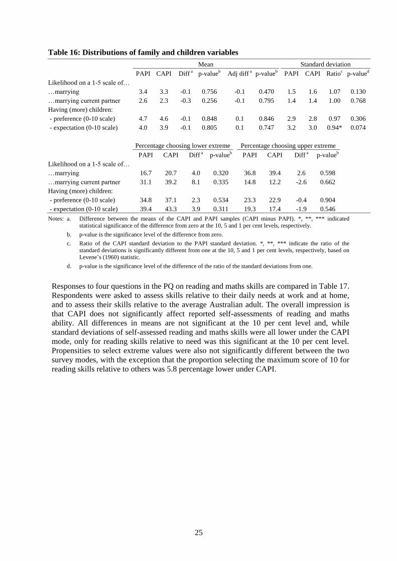
25

Table 16: Distributions of family and children variables


PAPI CAPI Diff a

p-valueb

Adj diff a

p-valueb

PAPI CAPI Ratioc

p-valued

Likelihood on a 1-5 scale of…

…marrying 3.4 3.3 -0.1 0.756 -0.1 0.470 1.5 1.6 1.07 0.130

…marrying current partner 2.6 2.3 -0.3 0.256 -0.1 0.795 1.4 1.4 1.00 0.768

Having (more) children:

- preference (0-10 scale) 4.7 4.6 -0.1 0.848 0.1 0.846 2.9 2.8 0.97 0.306

- expectation (0-10 scale) 4.0 3.9 -0.1 0.805 0.1 0.747 3.2 3.0 0.94* 0.074


PAPI CAPI Diff a

p-valueb

PAPI CAPI Diff a

p-valueb

Likelihood on a 1-5 scale of…

…marrying 16.7 20.7 4.0 0.320 36.8 39.4 2.6 0.598

…marrying current partner 31.1 39.2 8.1 0.335 14.8 12.2 -2.6 0.662

Having (more) children:

- preference (0-10 scale) 34.8 37.1 2.3 0.534 23.3 22.9 -0.4 0.904

- expectation (0-10 scale) 39.4 43.3 3.9 0.311 19.3 17.4 -1.9 0.546






Levene’s (1960) statistic.


Responses to four questions in the PQ on reading and maths skills are compared in Table 17.

Respondents were asked to assess skills relative to their daily needs at work and at home,

and to assess their skills relative to the average Australian adult. The overall impression is

that CAPI does not significantly affect reported self-assessments of reading and maths

ability. All differences in means are not significant at the 10 per cent level and, while

standard deviations of self-assessed reading and maths skills were all lower under the CAPI

mode, only for reading skills relative to need was this significant at the 10 per cent level.

Propensities to select extreme values were also not significantly different between the two

survey modes, with the exception that the proportion selecting the maximum score of 10 for

reading skills relative to others was 5.8 percentage lower under CAPI.

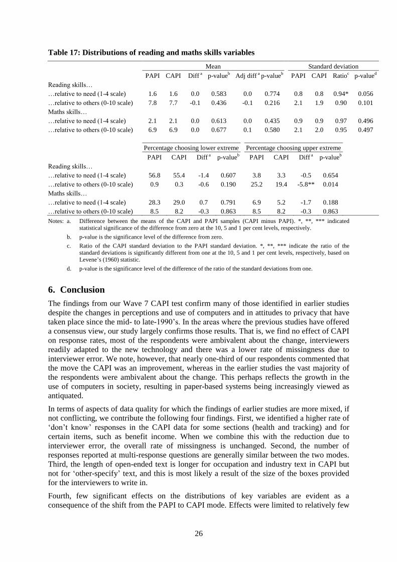
26

Table 17: Distributions of reading and maths skills variables


PAPI CAPI Diff a

p-valueb

Adj diff a

p-valueb

PAPI CAPI Ratioc

p-valued

Reading skills…

…relative to need (1-4 scale) 1.6 1.6 0.0 0.583 0.0 0.774 0.8 0.8 0.94* 0.056

…relative to others (0-10 scale) 7.8 7.7 -0.1 0.436 -0.1 0.216 2.1 1.9 0.90 0.101

Maths skills…

…relative to need (1-4 scale) 2.1 2.1 0.0 0.613 0.0 0.435 0.9 0.9 0.97 0.496

…relative to others (0-10 scale) 6.9 6.9 0.0 0.677 0.1 0.580 2.1 2.0 0.95 0.497


PAPI CAPI Diff a

p-valueb

PAPI CAPI Diff a

p-valueb

Reading skills…

…relative to need (1-4 scale) 56.8 55.4 -1.4 0.607 3.8 3.3 -0.5 0.654

…relative to others (0-10 scale) 0.9 0.3 -0.6 0.190 25.2 19.4 -5.8** 0.014

Maths skills…

…relative to need (1-4 scale) 28.3 29.0 0.7 0.791 6.9 5.2 -1.7 0.188

…relative to others (0-10 scale) 8.5 8.2 -0.3 0.863 8.5 8.2 -0.3 0.863






Levene’s (1960) statistic.


6. Conclusion

The findings from our Wave 7 CAPI test confirm many of those identified in earlier studies

despite the changes in perceptions and use of computers and in attitudes to privacy that have

taken place since the mid- to late-1990’s. In the areas where the previous studies have offered

a consensus view, our study largely confirms those results. That is, we find no effect of CAPI

on response rates, most of the respondents were ambivalent about the change, interviewers

readily adapted to the new technology and there was a lower rate of missingness due to

interviewer error. We note, however, that nearly one-third of our respondents commented that

the move the CAPI was an improvement, whereas in the earlier studies the vast majority of

the respondents were ambivalent about the change. This perhaps reflects the growth in the

use of computers in society, resulting in paper-based systems being increasingly viewed as

antiquated.

In terms of aspects of data quality for which the findings of earlier studies are more mixed, if

not conflicting, we contribute the following four findings. First, we identified a higher rate of

‘don’t know’ responses in the CAPI data for some sections (health and tracking) and for

certain items, such as benefit income. When we combine this with the reduction due to

interviewer error, the overall rate of missingness is unchanged. Second, the number of

responses reported at multi-response questions are generally similar between the two modes.

Third, the length of open-ended text is longer for occupation and industry text in CAPI but

not for ‘other-specify’ text, and this is most likely a result of the size of the boxes provided

for the interviewers to write in.

Fourth, few significant effects on the distributions of key variables are evident as a

consequence of the shift from the PAPI to CAPI mode. Effects were limited to relatively few

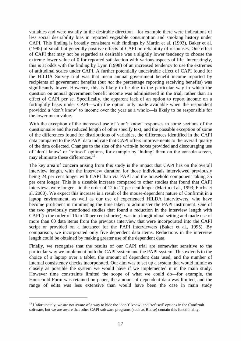
27

variables and were usually in the desirable direction—for example there were indications of

less social desirability bias in reported vegetable consumption and smoking history under

CAPI. This finding is broadly consistent with findings by Martin et al. (1993), Baker et al.

(1995) of small but generally positive effects of CAPI on reliability of responses. One effect

of CAPI that may not be regarded as desirable was a slightly lower tendency to choose the

extreme lower value of 0 for reported satisfaction with various aspects of life. Interestingly,

this is at odds with the finding by Lynn (1998) of an increased tendency to use the extremes

of attitudinal scales under CAPI. A further potentially undesirable effect of CAPI found for

the HILDA Survey trial was that mean annual government benefit income reported by

recipients of government benefits (but not the percentage reporting receiving benefits) was

significantly lower. However, this is likely to be due to the particular way in which the

question on annual government benefit income was administered in the trial, rather than an

effect of CAPI per se. Specifically, the apparent lack of an option to report income on a

fortnightly basis under CAPI—with the option only made available when the respondent

provided a ‘don’t know’ to income over the year as a whole—is likely to be responsible for

the lower mean value.

With the exception of the increased use of ‘don’t know’ responses in some sections of the

questionnaire and the reduced length of other specify text, and the possible exception of some

of the differences found for distributions of variables, the differences identified in the CAPI

data compared to the PAPI data indicate that CAPI offers improvements to the overall quality

of the data collected. Changes to the size of the write-in boxes provided and discouraging use

of ‘don’t know’ or ‘refused’ options, for example by ‘hiding’ them on the console screen,

may eliminate these differences.13

The key area of concern arising from this study is the impact that CAPI has on the overall

interview length, with the interview duration for those individuals interviewed previously

being 24 per cent longer with CAPI than via PAPI and the household component taking 35

per cent longer. This is a sizeable increase compared to other studies that found that CAPI

interviews were longer – in the order of 12 to 17 per cent longer (Martin el al., 1993; Fuchs et

al. 2000). We expect this increase is a result of the mouse-dependent nature of Confirmit in a

laptop environment, as well as our use of experienced HILDA interviewers, who have

become proficient in minimising the time taken to administer the PAPI instrument. One of

the two previously mentioned studies that found a reduction in the interview length with

CAPI (in the order of 16 to 20 per cent shorter), was in a longitudinal setting and made use of

more than 60 data items from the previous interview that were incorporated into the CAPI

script or provided on a factsheet for the PAPI interviewers (Baker et al., 1995). By

comparison, we incorporated only five dependent data items. Reductions in the interview

length could be obtained by making greater use of the dependent data.

Finally, we recognise that the results of our CAPI trial are somewhat sensitive to the

particular way we implement both the CAPI system and the PAPI system. This extends to the

choice of a laptop over a tablet, the amount of dependent data used, and the number of

internal consistency checks incorporated. Our aim was to set up a system that would mimic as

closely as possible the system we would have if we implemented it in the main study.

However time constraints limited the scope of what we could do—for example, the

Household Form was retained on paper, the amount of dependent data was limited, and the

range of edits was less extensive than would have been the case in main study

13

Unfortunately, we are not aware of a way to hide the ‘don’t’ know’ and ‘refused’ options in the Confirmit

software, but we are aware that other CAPI software programs (such as Blaise) contain this functionality.

28

implementation. Apart from the interviewer learning effects that are evident in the interview

lengths, there were also learning effects at the programming and management level which

would lead to improvements in CAPI implementation and fieldwork monitoring.

Nevertheless, the findings of this CAPI trial provides some solid contemporary information

for implementation of a full-scale CAPI system—and indeed it did provide valuable guidance

for the CAPI system implemented in Wave 9 of the HILDA Survey.

References

ABS (2004), ‘Labour Force: Australia, August 2004’, ABS Cat. No. 6202.0, Canberra.

Baker, R.P., Bradburn, N.M., and Johnson, R.A. (1995), ‘Computer-assisted Personal

Interviewing: An experimental evaluation of data quality and costs’, Journal of Official

Statistics, Vol. 11, No. 4, pp. 413-431.

Barresi, J., Finlay, D., and Sutcliffe, A. (2002), ‘CAI screen design project’, Methodology

Advisory Committee paper, Australian Bureau of Statistics, Canberra.

Couper, M.P. (2000), ‘Usability evaluation of computer-assisted survey instruments’, Social

Science Computer Review, Vol. 18, No. 4, pp. 384-396.

Couper, M.P., and Nicholls II, W.L. (1998), ‘The history and development of computer

assisted survey information collection methods’, in Couper, M.P. et al., editor, Computer

Assisted Survey Information Collection, Wiley, New York.

Dielman, L. and Couper, M.P. (1995), ‘Data quality in a CAPI survey: Keying errors’,

Journal of Official Statistics, Vol. 11, No. 2, pp. 141-146.

Banks, R. and Laurie, H. (2000), ‘From PAPI to CAPI: The case of the British Household

Panel Survey’, Social Science Computer Review, Vol. 18, No. 4, pp. 397-406.

de Leeuw, E., Hox, J., and Snijkers, G. (1995), ‘The effect of computer-assisted interviewing

on data quality’, Journal of the Market Research Society, Vol. 37, No. 4, pp. 325-344.

Fuchs, M., Couper, M. and Hansen, S.E. (2000), ‘Technology effects: Do CAPI or PAPI

interviews take longer?’, Journal of Official Statistics, vol. 16,no. 3., pp. 273-286.

Jäckle, A. (2008), ‘Dependent Interviewing: Effects on Respondent Burden and Efficiency of

Data Collection’, Journal of Official Statistics, Vol. 24, No. 3, pp. 411-430.

Headey, B. (2003), ‘How Best To Impute Taxes And Measure Public Transfers?’, HILDA

Discussion Paper Series No. 2/10, Melbourne Institute of Applied Economic and Social

Research, University of Melbourne.

Laurie, H. (2003), ‘From PAPI to CAPI: Consequences for data quality on the British

Household Panel Survey’, Working Papers of the Institute for Social and Economic Research,

No. 2003-14, University of Essex, Colchester.

Lepkowski, J.M., Sadosky, S.A., and Weiss, P.S. (1998), ‘Mode, behaviour, and data

recording error’, in Couper, M.P. et al., editor, Computer Assisted Survey Information

Collection, Wiley, New York, pp. 367-388.

Lynn, P. (1998), ‘Data collection mode effects on responses to attitudinal questions’, Journal

of Official Statistics, Vol. 14, No. 2, pp. 1-14.

Martin, J., O’Muircheartaigh, C. and Curtice, J. (1993) ‘The use of CAPI for attitude surveys:

An experimental comparison with traditional methods’, Journal of Official Statistics, Vol. 9,

No. 3, pp. 641-661.

29

Nicoletti, C. and Peracchi, F. (2003), ‘Survey response and survey characteristcs: Micro-level

evidence from ECHP’, Economics and Statistics Discussion Paper No. 15/04.

Schräpler, J., Schupp, J., and Wagner, G.G. (2006), ‘Changing from PAPI to CAPI: A

longitudinal study of mode-effects based on an experimental design’, DIW Discussion Paper

No. 593, Berlin.

Tourangeau, R, and Smith, T. (1996), ‘Asking sensitive questions’, Public Opinion

Quarterly, Vol. 60, pp. 275-304.

van Bastelaer, A., Kerssemakers, F., and Sikkel, D. (1988), ‘Data collection with hand-held

computers: Contributions to questionnaire design’, Journal of Official Statistics, Vol. 4, No.

2, pp. 141-154.

Watson, N. (2010), ‘The impact of the transition to CAPI and a new fieldwork provider on

the HILDA Survey’, HILDA Discussion Paper Series No. 2/10, Melbourne Institute of

Applied Economic and Social Research, University of Melbourne.

Wooden, M. and Watson, N. (2007), ‘The HILDA Survey and its Contribution to Economic

and Social Research (So Far)’, The Economic Record, vol. 83, no. 261, pp. 208–231.

Documents

HILDA PROJECT DISCUSSION PAPER SERIES No. … · HILDA PROJECT DISCUSSION PAPER SERIES ... checking inconsistencies in the data with the respondent as ... requiring choice of a position