Embed Size (px)
Citation preview
Hilary Hoynes UC Davis 230A Lecture: Effects of income on health and other outcomes Gordon Dahl and Lance Lochner, “The Impact of Family Income on Child Achievement: Evidence from Changes in the Earned Income Tax Credit”, American Economic Review 2012 Hoynes, Miller and Simon, “Income, the Earned Income Tax Credit, and Infant Health,”mimeo Evans and Garthwaite “Giving Mom a Break: The Impact of Higher EITC Payments on Maternal Health?
Effect of Income on Outcomes
• Does money matter? First order important. • Challenge: endogeneity of income • Cross section: low income may be correlated with other
“bads” (neighborhood, family stability, schools) • Changes (family FE models): year to year changes in
family income (e.g. job change, job loss) may also change other outcomes in the family.
• A few recent papers use the EITC as a plausibly credible source of exogenous variation in (after tax) income.
• Also part of a growing literature that examines the health impacts of non-health programs and interventions
Other studies with credible-designs of income and health
• Impacts on adult mortality using shocks to income: – Social security payments (Snyder and Evans 2005): social security
notch – Agricultural income (Banerjee et al., 2007): disease to wine crop
leading to shocks to birth year – province income in childhood – South African pensions (Case 2004) – Inheritance (Meer, Miller and Rosen, 2003)
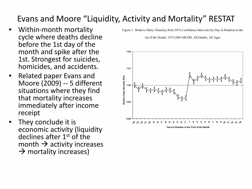
Evans and Moore “Liquidity, Activity and Mortality” RESTAT • Within-month mortality
cycle where deaths decline before the 1st day of the month and spike after the 1st. Strongest for suicides, homicides, and accidents.
• Related paper Evans and Moore (2009) -- 5 different situations where they find that mortality increases immediately after income receipt
• They conclude it is economic activity (liquidity declines after 1st of the month activity increases mortality increases)
Other studies with credible-designs of income and health
• Income support programs: – Rollout of food stamps (Almond, Hoynes and Schanzenbach 2011) and
WIC (Hoynes, Page and Stevens 2011) leads to improvement in infant health.
– Conditional cash transfer programs improve infant health: Amarante et al (2011), Barber and Gertler (2008).
Other studies with credible-designs of income and health
• Recessions and business cycles – Infant health decreases in recessions due in part to selection of
mothers (Dehejia and Lleras-Muney 2004) – Infant health rises with layoffs (Lindo 2011). – Mortality is pro-cyclical (Ruhn). Stevens et al (2012) show that it is
concentrated among the oldest old; due to labor market for nursing home workers (tight labor market turnover / staffing problems higher mortality)
Other studies with credible-designs of income and health
• Mixed evidence whether maternal education increases infant health (Currie and Moretti 2003 -- Yes; McCrary and Royer 2010 – No)
• Milligan and Stabile (2009) use variation across Canadian provinces in child tax benefits – find improvement in child outcomes
• Løken 2010, Løken, Mogstad and Wiswall 2010 use variation in economic boom following Norway’s oil discovery and find increases in education and IQ.
EITC, Income and Incentives
• EITC leads to increase in after-tax income due to tax refund (or reduction in tax liability)
• The EITC requires earned income for single earners incentivizes employment increase in income but reduction in time with children
• The EITC increases with number of children may incentivize fertility (but more work may lead to opposite prediction) – Weak and small impacts on fertility (Baughman and Dickert-
Conlin, 2009) • Complex incentives for marriage (depends on who has
the children and who has the earnings) – Weak and small impacts on marriage (Eissa and Hoynes 2004,
Dickert-Conlin 2002, Ellwood 2000, Herbst 2011)
Possible channels: EITC and Infant Health (or child development)
Increases in infant health: • Child health is a normal good (more income better inputs) • More income increases well being of mother [lower stress, Evans
and Garthwaite 2010] which may improve infant health [Aizer et al 2009, Camacho 2009]
Uncertain effects on infant health: • Increase in work ? Infant health [mixed evidence: Baum 2005,Del
Bono et al 2008, Gelber and Mitchell 2011—EITC reduces leisure and home production but no effect on child time ]
• Changes in fertility (composition effect) , probably negative if low SES women increase fertility
Decreases in infant health • Income could increase spending on bad inputs, e.g. smoking
and drinking
The New Biology of Poverty: SES, Stress and Cortisol
• It has been known for some time that socio-economic status (SES) is correlated with self-reported stress and the stress-hormone cortisol.
• Cortisol is released in response to both psychological and physiological strain. Chronic elevations of cortisol can lead to dysfunction in metabolic and immune systems (Sterling and Eyer 1988; McEwan and Stellar,
1993; McEwen, 1998) and this stress may accelerate cell aging (Epel et al., 2004; Cherkas et al., 2006).
10
• Exciting new research suggests a causal linkage: – Conditional cash transfers (Oportunidades in rural Mexico)
lead to reduction in cortisol among children 2-6 (Fernald and Gunnar 2009)
– Negative rainfall shocks lead to higher cortisol in Kenya (Haushofer et al 2012)
– Expansion of in-work benefits (EITC) lowers risky biomarkers in mothers (Evans and Garthwaite 2011)
– Prenatal maternal cortisol negatively affects the health, cognition, and education of children (Aizer, Stroud and Buka 2009)
• This suggests that increases in income – through government policy – can reduce cortisol. 11
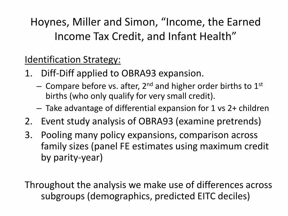
Hoynes, Miller and Simon, “Income, the Earned Income Tax Credit, and Infant Health”
Identification Strategy: 1. Diff-Diff applied to OBRA93 expansion.
– Compare before vs. after, 2nd and higher order births to 1st births (who only qualify for very small credit).
– Take advantage of differential expansion for 1 vs 2+ children 2. Event study analysis of OBRA93 (examine pretrends) 3. Pooling many policy expansions, comparison across
family sizes (panel FE estimates using maximum credit by parity-year)
Throughout the analysis we make use of differences across
subgroups (demographics, predicted EITC deciles)
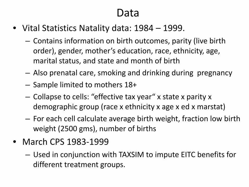
Data • Vital Statistics Natality data: 1984 – 1999.
– Contains information on birth outcomes, parity (live birth order), gender, mother’s education, race, ethnicity, age, marital status, and state and month of birth
– Also prenatal care, smoking and drinking during pregnancy – Sample limited to mothers 18+ – Collapse to cells: “effective tax year“ x state x parity x
demographic group (race x ethnicity x age x ed x marstat) – For each cell calculate average birth weight, fraction low birth
weight (2500 gms), number of births
• March CPS 1983-1999 – Used in conjunction with TAXSIM to impute EITC benefits for
different treatment groups.
14
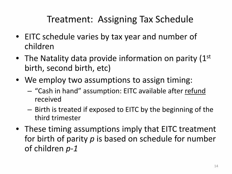
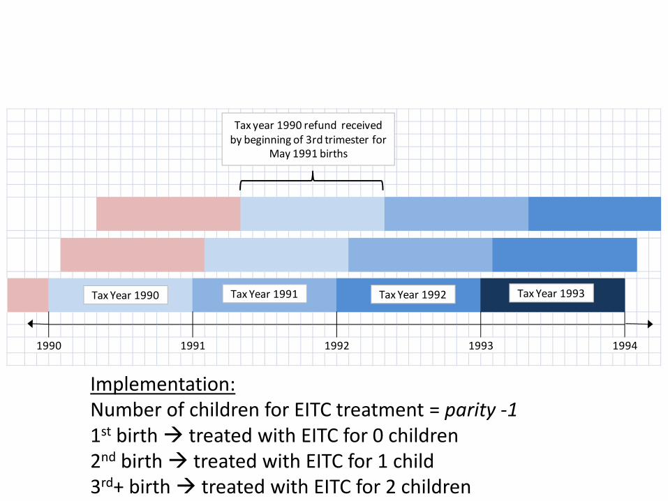
Treatment: Assigning Tax Schedule
• EITC schedule varies by tax year and number of children
• The Natality data provide information on parity (1st birth, second birth, etc)
• We employ two assumptions to assign timing: – “Cash in hand” assumption: EITC available after refund
received – Birth is treated if exposed to EITC by the beginning of the
third trimester • These timing assumptions imply that EITC treatment
for birth of parity p is based on schedule for number of children p-1
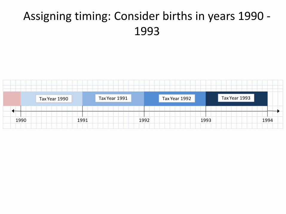
Assigning timing: Consider births in years 1990 - 1993
1992 1993 199419911990
Tax Year 1990 Tax Year 1991 Tax Year 1992 Tax Year 1993
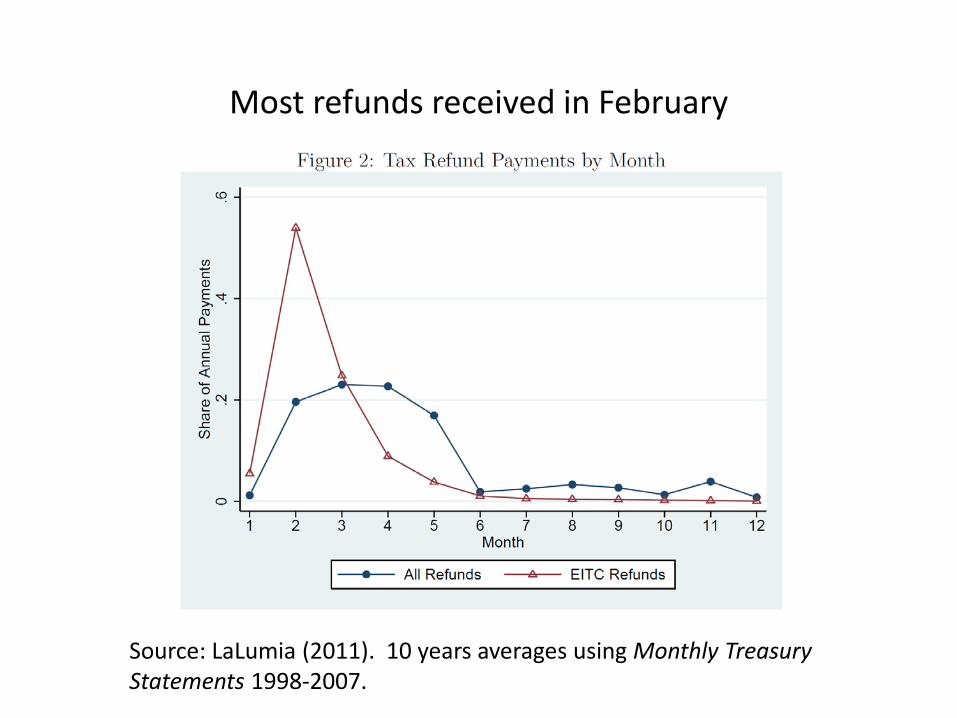
Source: LaLumia (2011). 10 years averages using Monthly Treasury Statements 1998-2007.
Most refunds received in February
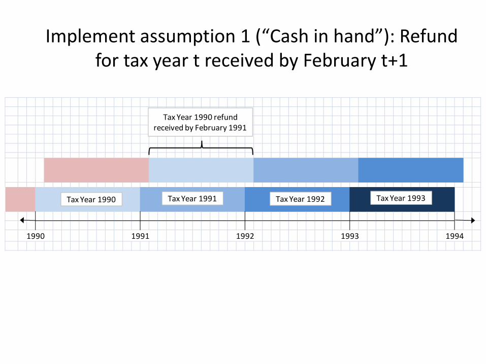
Implement assumption 1 (“Cash in hand”): Refund for tax year t received by February t+1
1990 1991 1992 1993 1994
Tax Year 1990 Tax Year 1991 Tax Year 1992 Tax Year 1993
Tax Year 1990 refundreceived by February 1991
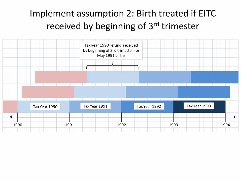
Implement assumption 2: Birth treated if EITC received by beginning of 3rd trimester
1990 1991 1992 1993 1994
Tax Year 1990 Tax Year 1991 Tax Year 1992 Tax Year 1993
Tax year 1990 refund received by beginning of 3rd trimester for
May 1991 births
1990 1991 1992 1993 1994
Tax Year 1990 Tax Year 1991 Tax Year 1992 Tax Year 1993
Tax year 1990 refund received by beginning of 3rd trimester for
May 1991 births
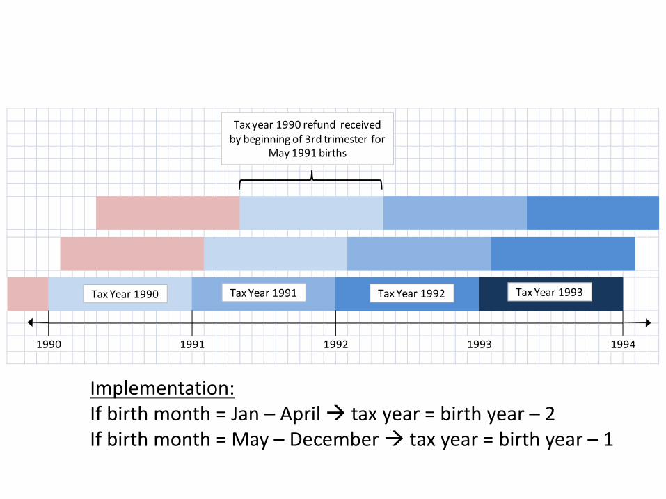
Implementation: If birth month = Jan – April tax year = birth year – 2 If birth month = May – December tax year = birth year – 1
1990 1991 1992 1993 1994
Tax Year 1990 Tax Year 1991 Tax Year 1992 Tax Year 1993
Tax year 1990 refund received by beginning of 3rd trimester for
May 1991 births
Implementation: Number of children for EITC treatment = parity -1 1st birth treated with EITC for 0 children 2nd birth treated with EITC for 1 child 3rd+ birth treated with EITC for 2 children
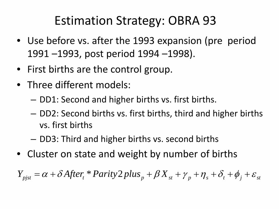
Estimation Strategy: OBRA 93 • Use before vs. after the 1993 expansion (pre period
1991 –1993, post period 1994 –1998). • First births are the control group. • Three different models:
– DD1: Second and higher births vs. first births. – DD2: Second births vs. first births, third and higher births
vs. first births – DD3: Third and higher births vs. second births
• Cluster on state and weight by number of births
* 2pjst t p st p s t j stY After Parity plus Xα δ β γ η δ φ ε= + + + + + + +
$0
$500
$1,000
$1,500
$2,000
$2,500
$3,000
$3,500
$4,000
$4,500
1983 1985 1987 1989 1991 1993 1995 1997 1999
Tax Year
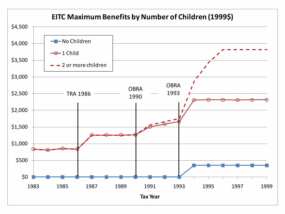
EITC Maximum Benefits by Number of Children (1999$)
No Children
1 Child
2 or more children
TRA 1986OBRA1993
OBRA1990TRA 1986
OBRA1993
OBRA1990
High impact sample • Our main results are for single women with a high
school education or less • This sample is commonly used in the EITC literature • We will also show results for broader samples, and
placebo groups • We focus on percent low birth weight as our main
outcome
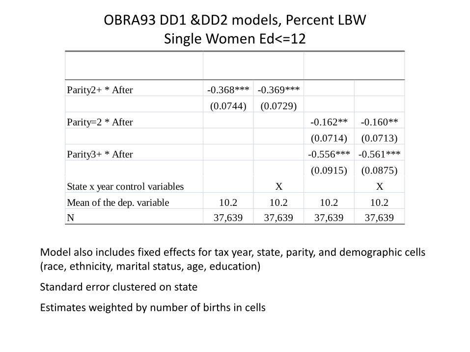
OBRA93 DD1 &DD2 models, Percent LBW Single Women Ed<=12
Model also includes fixed effects for tax year, state, parity, and demographic cells (race, ethnicity, marital status, age, education)
Standard error clustered on state
Estimates weighted by number of births in cells
Parity2+ * After -0.368*** -0.369***(0.0744) (0.0729)
Parity=2 * After -0.162** -0.160**(0.0714) (0.0713)
Parity3+ * After -0.556*** -0.561***(0.0915) (0.0875)
State x year control variables X XMean of the dep. variable 10.2 10.2 10.2 10.2N 37,639 37,639 37,639 37,639
Event time analysis
• Replace pre/post analysis with year by year comparison of the treated vs. control group
• Advantages: – Estimate pre-trends; test for validity of the design – Examine overtime pattern of treatment effect
• Practically: replace After and Parity dummies with full set of year dummies and year dummies interacted with Parity
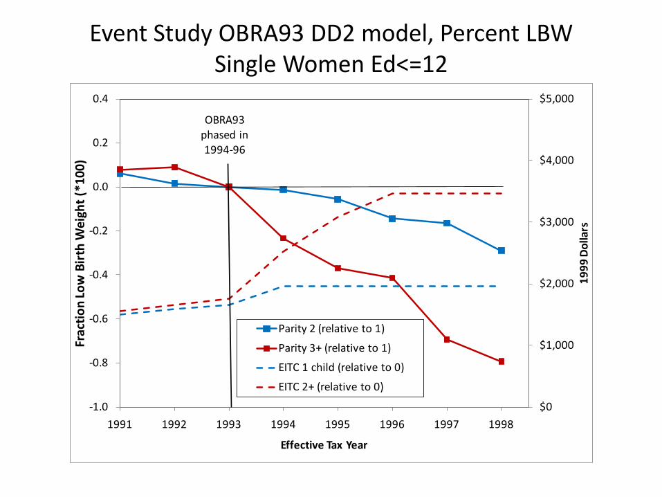
Event Study OBRA93 DD2 model, Percent LBW Single Women Ed<=12
$0
$1,000
$2,000
$3,000
$4,000
$5,000
-1.0
-0.8
-0.6
-0.4
-0.2
0.0
0.2
0.4
1991 1992 1993 1994 1995 1996 1997 1998
1999
Dol
lars
Frac
tion
Low
Birt
h W
eigh
t (*1
00)
Effective Tax Year
Parity 2 (relative to 1)
Parity 3+ (relative to 1)
EITC 1 child (relative to 0)
EITC 2+ (relative to 0)
OBRA93phased in 1994-96
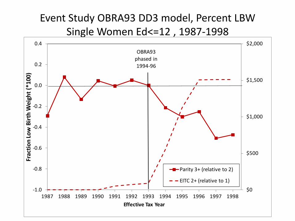
Event Study OBRA93 DD3 model, Percent LBW Single Women Ed<=12 , 1987-1998
$0
$500
$1,000
$1,500
$2,000
-1.0
-0.8
-0.6
-0.4
-0.2
0.0
0.2
0.4
1987 1988 1989 1990 1991 1992 1993 1994 1995 1996 1997 1998
Frac
tion
Low
Birt
h W
eigh
t (*1
00)
Effective Tax Year
Parity 3+ (relative to 2)
EITC 2+ (relative to 1)
OBRA93phased in 1994-96
Magnitudes: Interpreting the Reduced Form
• We use the 1993-1999 March CPS combined with TAXSIM to impute the magnitude of the OBRA93 EITC “treatment” – Sample of women 18-45 with children<3 (proxy for “new
births sample”) – Use observed marital status and number of children to
assign tax schedule for effective tax year – Impute EITC using TAXSIM (using CPS earnings/income)
• Estimate difference-in-difference impact on EITC income (e.g. by parity and pre/post) OBRA93 EITC treatment
• Assume effects operate through EITC $ amount
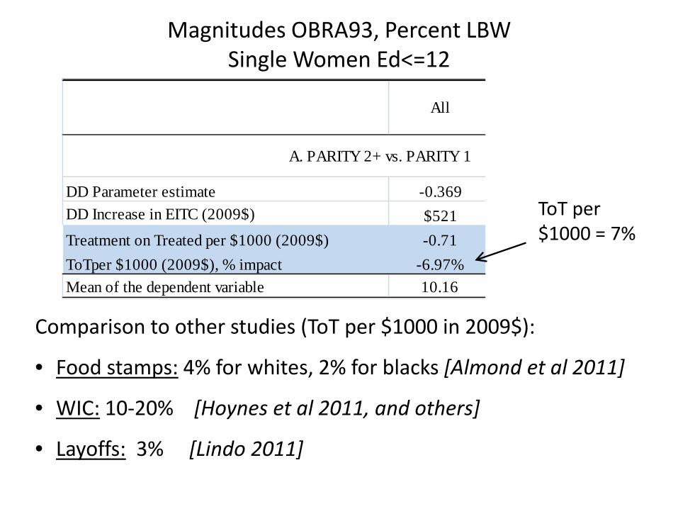
Magnitudes OBRA93, Percent LBW Single Women Ed<=12
All White Black
DD Parameter estimate -0.369 -0.169 -0.741DD Increase in EITC (2009$) $521 $471 $624Treatment on Treated per $1000 (2009$) -0.71 -0.36 -1.19ToTper $1000 (2009$), % impact -6.97% -4.41% -8.23%Mean of the dependent variable 10.16 8.14 14.43
A. PARITY 2+ vs. PARITY 1
Comparison to other studies (ToT per $1000 in 2009$):
• Food stamps: 4% for whites, 2% for blacks [Almond et al 2011]
• WIC: 10-20% [Hoynes et al 2011, and others]
• Layoffs: 3% [Lindo 2011]
ToT per $1000 = 7%
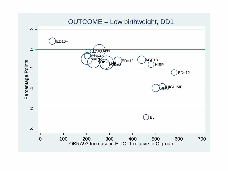
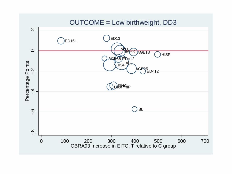
Subgroup Analysis
• Thus far we have shown average treatment effects for our high impact sample
• The likelihood of being impacted the EITC varies across groups.
• We use the full sample and estimate the same models on subgroups: race (white, black), ethnicity (Hispanic), Non-Hispanic), age (18-24, 25-34, 35+), education (<12,=12,13-15,16+), marital status (married, single), and (for continuity) the high impact sample.
• We use the CPS and TAXSIM to calculate the DD impact on EITC income as above.
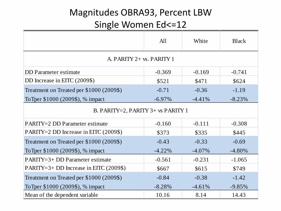
Magnitudes OBRA93, Percent LBW Single Women Ed<=12
All White Black
DD Parameter estimate -0.369 -0.169 -0.741DD Increase in EITC (2009$) $521 $471 $624Treatment on Treated per $1000 (2009$) -0.71 -0.36 -1.19ToTper $1000 (2009$), % impact -6.97% -4.41% -8.23%
PARITY=2 DD Parameter estimate -0.160 -0.111 -0.308PARITY=2 DD Increase in EITC (2009$) $373 $335 $445Treatment on Treated per $1000 (2009$) -0.43 -0.33 -0.69ToTper $1000 (2009$), % impact -4.22% -4.07% -4.80%PARITY=3+ DD Parameter estimate -0.561 -0.231 -1.065PARITY=3+ DD Increase in EITC (2009$) $667 $615 $749Treatment on Treated per $1000 (2009$) -0.84 -0.38 -1.42ToTper $1000 (2009$), % impact -8.28% -4.61% -9.85%Mean of the dependent variable 10.16 8.14 14.43
A. PARITY 2+ vs. PARITY 1
B. PARITY=2, PARITY 3+ vs PARITY 1
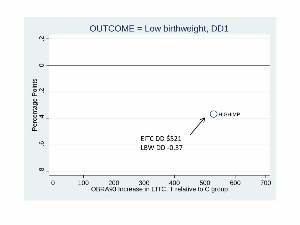
HIGHIMP
-.8-.6
-.4-.2
0.2
Per
cent
age
Poi
nts
0 100 200 300 400 500 600 700OBRA93 Increase in EITC, T relative to C group
OUTCOME = Low birthweight, DD1
EITC DD $521 LBW DD -0.37
ED16+
MARRED13AGE35
NHISP
WH
AGE25ALL ED=12 AGE18
BL
HISP
SINGHIGHIMP
ED<12
-.8-.6
-.4-.2
0.2
Per
cent
age
Poi
nts
0 100 200 300 400 500 600 700OBRA93 Increase in EITC, T relative to C group
OUTCOME = Low birthweight, DD1
ED16+
AGE35
ED13
NHISP
HIGHIMPSING
WH
ED=12
MARR
ALLAGE25
AGE18
BL
ED<12
HISP
-.8-.6
-.4-.2
0.2
Per
cent
age
Poi
nts
0 100 200 300 400 500 600 700OBRA93 Increase in EITC, T relative to C group
OUTCOME = Low birthweight, DD3
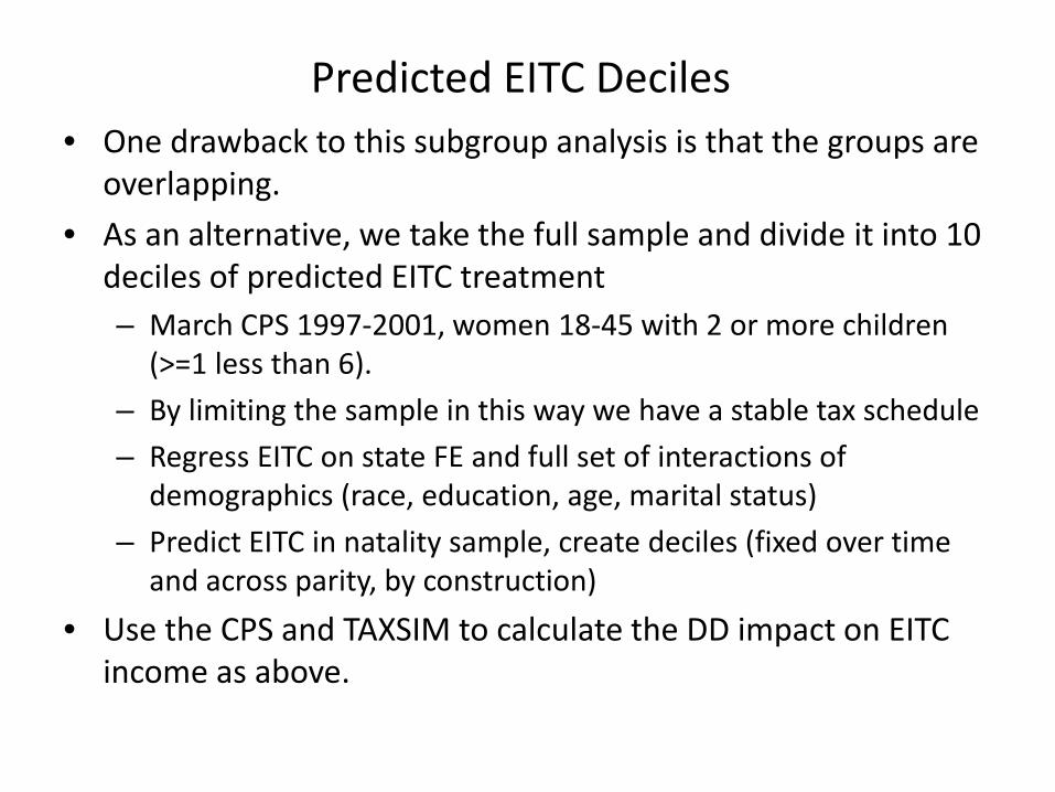
Predicted EITC Deciles • One drawback to this subgroup analysis is that the groups are
overlapping. • As an alternative, we take the full sample and divide it into 10
deciles of predicted EITC treatment – March CPS 1997-2001, women 18-45 with 2 or more children
(>=1 less than 6). – By limiting the sample in this way we have a stable tax schedule – Regress EITC on state FE and full set of interactions of
demographics (race, education, age, marital status) – Predict EITC in natality sample, create deciles (fixed over time
and across parity, by construction) • Use the CPS and TAXSIM to calculate the DD impact on EITC
income as above.
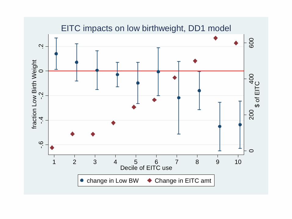
020
040
060
0$
of E
ITC
-.6-.4
-.20
.2fra
ctio
n Lo
w B
irth
Wei
ght
1 2 3 4 5 6 7 8 9 10Decile of EITC use
change in Low BW Change in EITC amt
EITC impacts on low birthweight, DD1 model
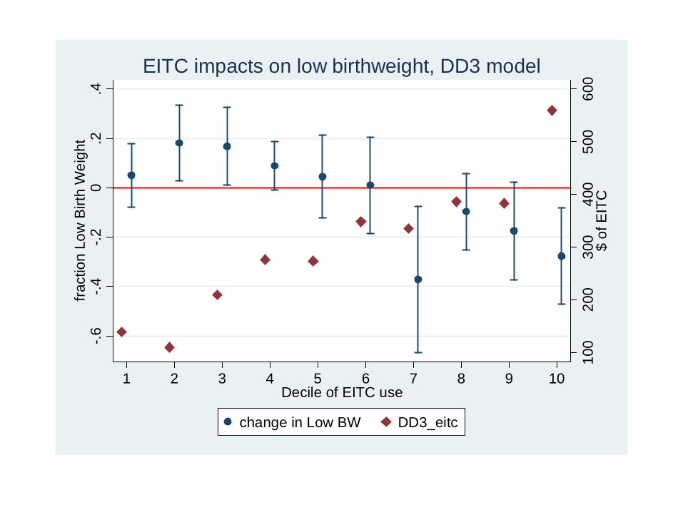
100
200
300
400
500
600
$ of
EIT
C
-.6-.4
-.20
.2.4
fract
ion
Low
Birt
h W
eigh
t
1 2 3 4 5 6 7 8 9 10Decile of EITC use
change in Low BW DD3_eitc
EITC impacts on low birthweight, DD3 model
Threats to the design: endogenous births
• If EITC changes fertility (composition of births) then the results could be biased [most likely downward]. – Increase in births among disadvantaged? – Increase in fetal survival?
• We apply the same identification strategy and examine impacts on number and composition of births.
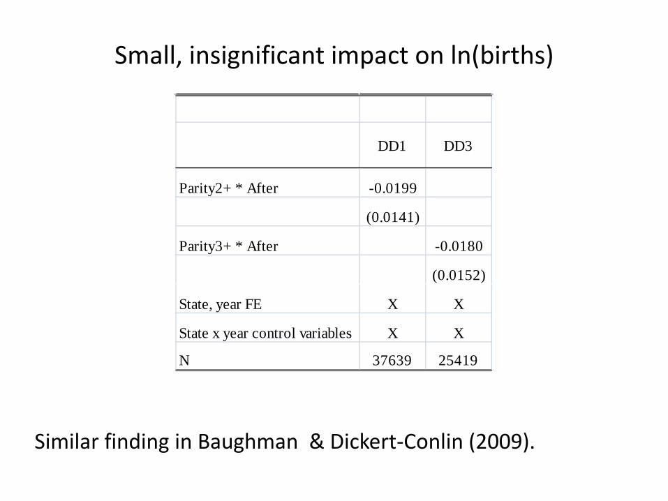
Small, insignificant impact on ln(births)
DD1 DD3
Parity2+ * After -0.0199
(0.0141)
Parity3+ * After -0.0180
(0.0152)
State, year FE X X
State x year control variables X X
N 37639 25419
Similar finding in Baughman & Dickert-Conlin (2009).
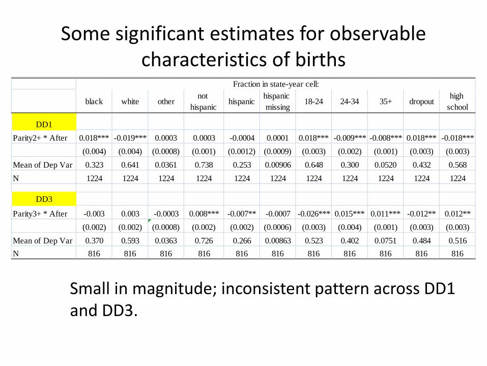
Some significant estimates for observable characteristics of births
Small in magnitude; inconsistent pattern across DD1 and DD3.
black white othernot
hispanichispanic
hispanic missing
18-24 24-34 35+ dropouthigh
school
DD1Parity2+ * After 0.018*** -0.019*** 0.0003 0.0003 -0.0004 0.0001 0.018*** -0.009*** -0.008*** 0.018*** -0.018***
(0.004) (0.004) (0.0008) (0.001) (0.0012) (0.0009) (0.003) (0.002) (0.001) (0.003) (0.003)Mean of Dep Var 0.323 0.641 0.0361 0.738 0.253 0.00906 0.648 0.300 0.0520 0.432 0.568N 1224 1224 1224 1224 1224 1224 1224 1224 1224 1224 1224
DD3
Parity3+ * After -0.003 0.003 -0.0003 0.008*** -0.007** -0.0007 -0.026*** 0.015*** 0.011*** -0.012** 0.012**(0.002) (0.002) (0.0008) (0.002) (0.002) (0.0006) (0.003) (0.004) (0.001) (0.003) (0.003)
Mean of Dep Var 0.370 0.593 0.0363 0.726 0.266 0.00863 0.523 0.402 0.0751 0.484 0.516N 816 816 816 816 816 816 816 816 816 816 816
Fraction in state-year cell:
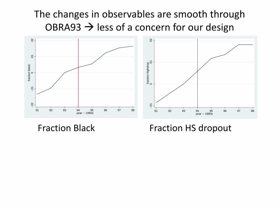
The changes in observables are smooth through OBRA93 less of a concern for our design
-.02
-.01
0.0
1.0
2fra
ctio
n bl
ack
91 92 93 94 95 96 97 98year -- 1990s
-.01
0.0
1.0
2fra
ctio
n hi
ghdr
op
91 92 93 94 95 96 97 98year -- 1990s
Fraction Black Fraction HS dropout
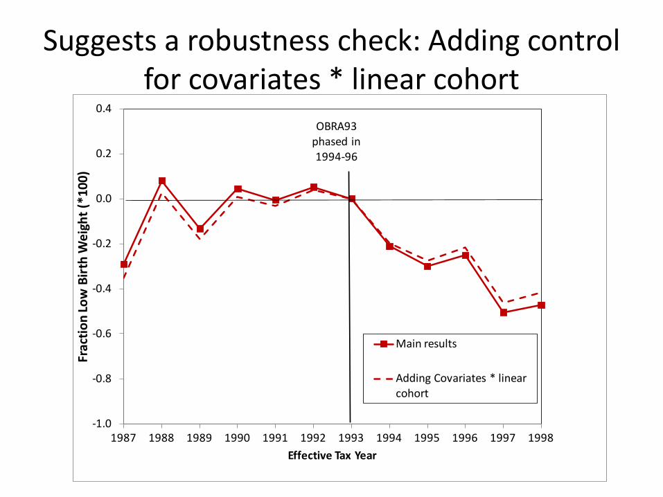
Suggests a robustness check: Adding control for covariates * linear cohort
-1.0
-0.8
-0.6
-0.4
-0.2
0.0
0.2
0.4
1987 1988 1989 1990 1991 1992 1993 1994 1995 1996 1997 1998
Frac
tion
Low
Birt
h W
eigh
t (*1
00)
Effective Tax Year
Main results
Adding Covariates * linear cohort
OBRA93phased in 1994-96
Evidence on possible mechanisms
• We take advantage of additional information on the birth certificate: prenatal care, any smoking during pregnancy, any drinking during pregnancy, gestation
• We estimate the same models as presented above.
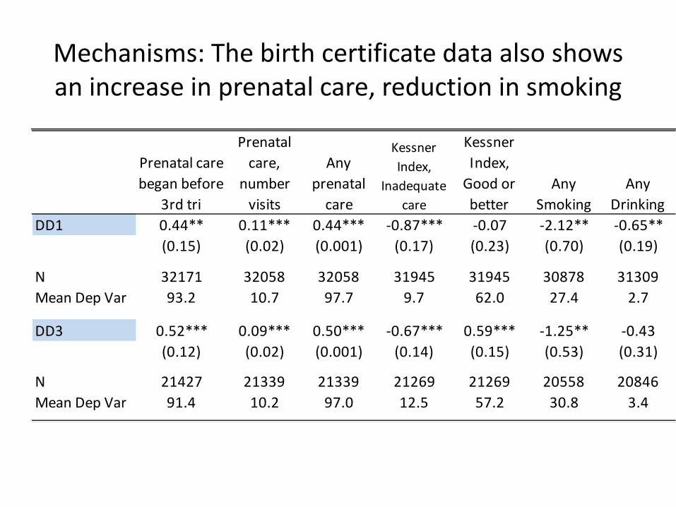
Mechanisms: The birth certificate data also shows an increase in prenatal care, reduction in smoking
Prenatal care began before
3rd tri
Prenatal care,
number visits
Any prenatal
care
Kessner Index,
Inadequate care
Kessner Index,
Good or better
Any Smoking
Any Drinking
DD1 0.44** 0.11*** 0.44*** -0.87*** -0.07 -2.12** -0.65**(0.15) (0.02) (0.001) (0.17) (0.23) (0.70) (0.19)
N 32171 32058 32058 31945 31945 30878 31309Mean Dep Var 93.2 10.7 97.7 9.7 62.0 27.4 2.7
DD3 0.52*** 0.09*** 0.50*** -0.67*** 0.59*** -1.25** -0.43(0.12) (0.02) (0.001) (0.14) (0.15) (0.53) (0.31)
N 21427 21339 21339 21269 21269 20558 20846Mean Dep Var 91.4 10.2 97.0 12.5 57.2 30.8 3.4
Exploring a possible role of health insurance
• We know that the EITC leads to an increase in the extensive margin of labor supply, and transitions from welfare to work
• We would expect a reduction in Medicaid coverage and, possibly, an increase in private health insurance
• To explore this, we use the March CPS 1991-1998 and construct treatment and control groups to match our OBRA analysis
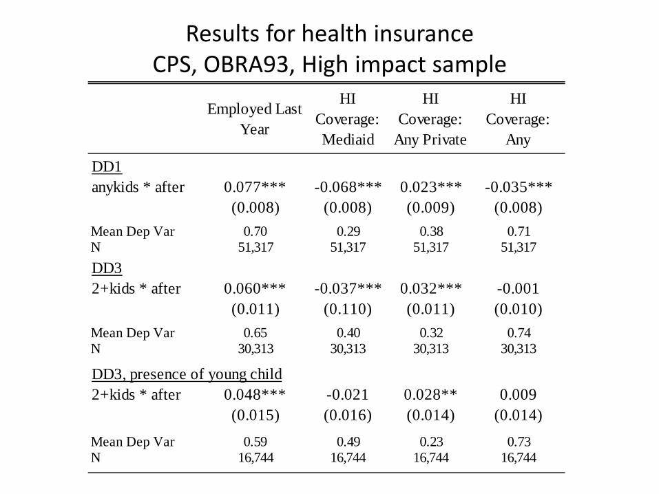
Results for health insurance CPS, OBRA93, High impact sample
Employed Last Year
HI Coverage: Mediaid
HI Coverage:
Any Private
HI Coverage:
Any
DD1anykids * after 0.077*** -0.068*** 0.023*** -0.035***
(0.008) (0.008) (0.009) (0.008)Mean Dep Var 0.70 0.29 0.38 0.71N 51,317 51,317 51,317 51,317DD32+kids * after 0.060*** -0.037*** 0.032*** -0.001
(0.011) (0.110) (0.011) (0.010)Mean Dep Var 0.65 0.40 0.32 0.74N 30,313 30,313 30,313 30,313
DD3, presence of young child2+kids * after 0.048*** -0.021 0.028** 0.009
(0.015) (0.016) (0.014) (0.014)
Mean Dep Var 0.59 0.49 0.23 0.73N 16,744 16,744 16,744 16,744
Mechanisms
• Increases in prenatal care and reductions in smoking are part of the pathway for our results for improving infant health
• This could be generated by additional income (affordability of prenatal care), employment (less smoking)
• Overall health insurance, if anything, declines. But there could be an effect for some of an “upgrading” due to the increase in private insurance
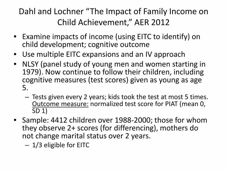
Dahl and Lochner “The Impact of Family Income on Child Achievement,” AER 2012
• Examine impacts of income (using EITC to identify) on child development; cognitive outcome
• Use multiple EITC expansions and an IV approach • NLSY (panel study of young men and women starting in
1979). Now continue to follow their children, including cognitive measures (test scores) given as young as age 5. – Tests given every 2 years; kids took the test at most 5 times.
Outcome measure: normalized test score for PIAT (mean 0, SD 1)
• Sample: 4412 children over 1988-2000; those for whom they observe 2+ scores (for differencing), mothers do not change marital status over 2 years. – 1/3 eligible for EITC
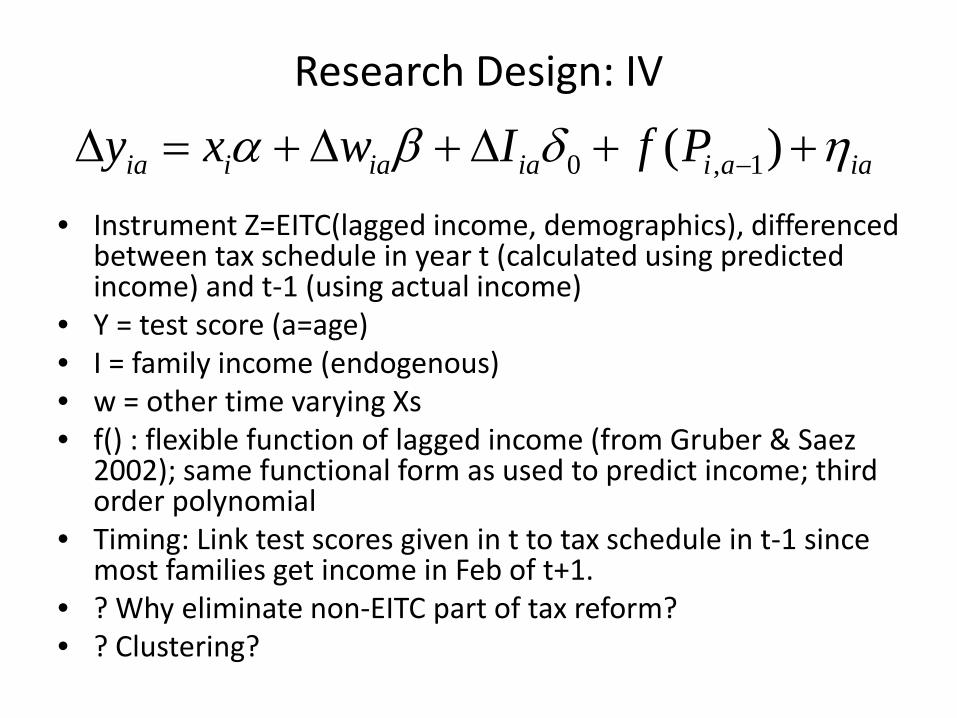
Research Design: IV
• Instrument Z=EITC(lagged income, demographics), differenced between tax schedule in year t (calculated using predicted income) and t-1 (using actual income)
• Y = test score (a=age) • I = family income (endogenous) • w = other time varying Xs • f() : flexible function of lagged income (from Gruber & Saez
2002); same functional form as used to predict income; third order polynomial
• Timing: Link test scores given in t to tax schedule in t-1 since most families get income in Feb of t+1.
• ? Why eliminate non-EITC part of tax reform? • ? Clustering?
0 , 1( )ia i ia ia i a iay x w I f Pα β δ η−∆ = + ∆ + ∆ + +
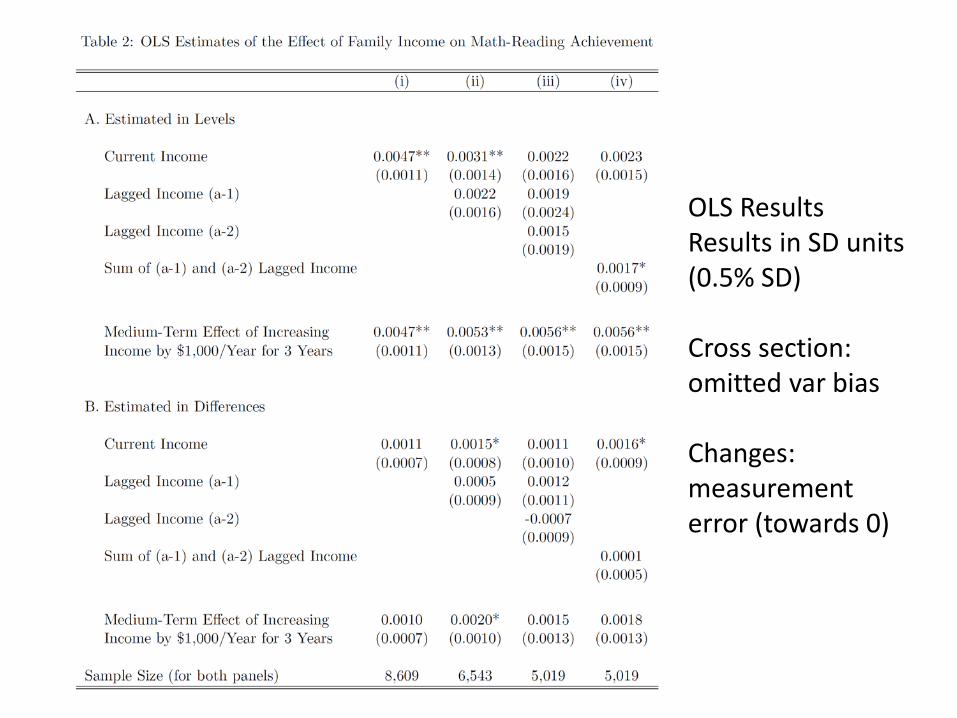
OLS Results Results in SD units (0.5% SD) Cross section: omitted var bias Changes: measurement error (towards 0)
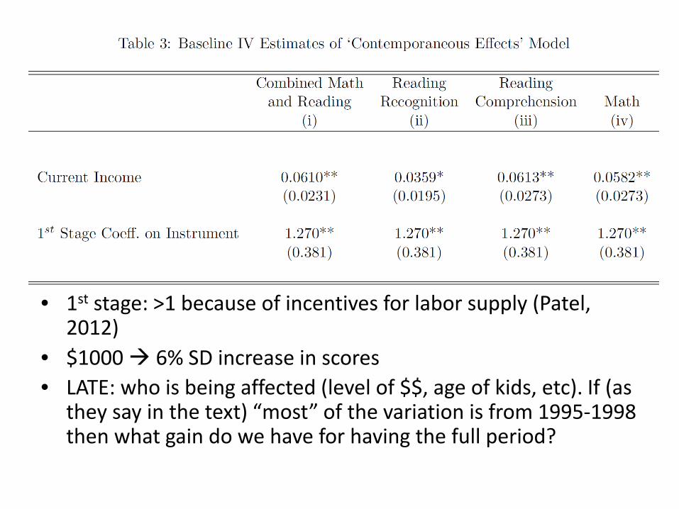
• 1st stage: >1 because of incentives for labor supply (Patel, 2012)
• $1000 6% SD increase in scores • LATE: who is being affected (level of $$, age of kids, etc). If (as
they say in the text) “most” of the variation is from 1995-1998 then what gain do we have for having the full period?
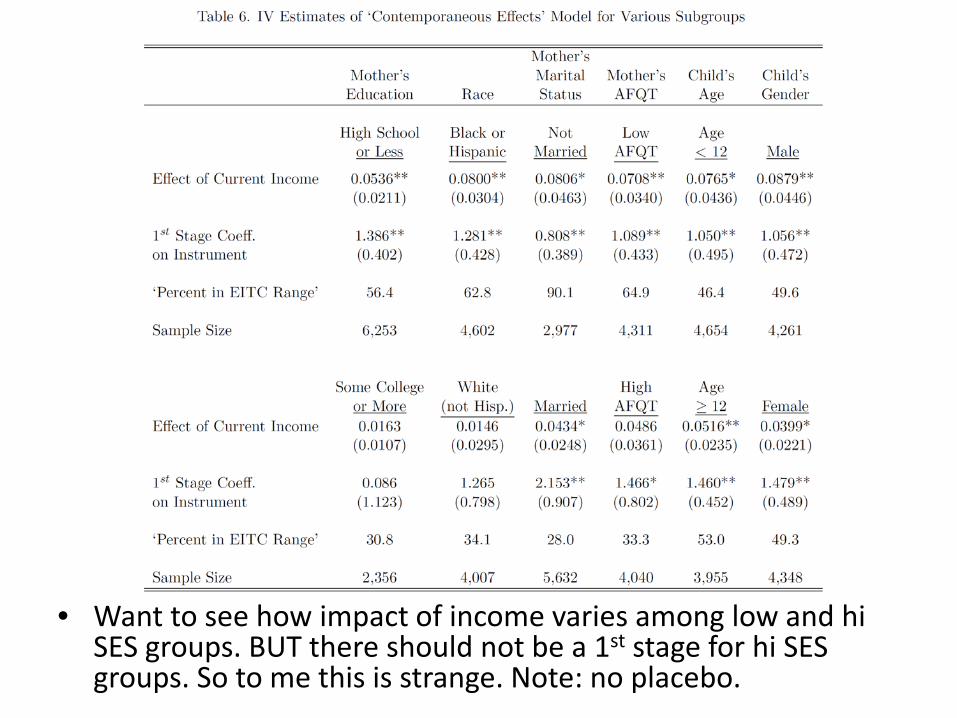
• Want to see how impact of income varies among low and hi SES groups. BUT there should not be a 1st stage for hi SES groups. So to me this is strange. Note: no placebo.
General challenge with EITC as instrument for income
• It also changes (single) women’s employment this could also affect the outcome. AND we only have one instrument.