Embed Size (px)
Citation preview
HIGHWAY TO HITLER*
Nico Voigtländer
UCLA and NBER
Hans‐Joachim Voth
University of Zurich and CEPR
First draft: February 2014
This draft: October 2014
Abstract: Can infrastructure investment win “hearts and minds”? We analyze a famous
case in the early stages of dictatorship – the building of the motorway network in Nazi
Germany. The Autobahn was one of the most important projects of the Hitler
government. It was intended to reduce unemployment, and was widely used for
propaganda purposes. We examine its role in increasing support for the Nazi regime by
analyzing new data on motorway construction and the 1934 plebiscite, which gave
Hitler greater powers as head of state. Our results suggest that road building was highly
effective, reducing opposition to the nascent Nazi regime.
Keywords: political economy, infrastructure spending, establishment of
dictatorships, pork‐barrel politics, Nazi regime
JEL Classification: H54, P16, N44, N94
* For helpful comments, we thank Paula Bustos, Julia Cage, Vasco Carvalho, Ruben Enikolopov,
Rick Hornbeck, Jose Luis Peydro, Diego Puga, Giacomo Ponzetto, Kurt Schmidheiny, Moritz
Schularick, and David Strömberg. Seminar audiences at Basel University, Bonn University, the
Juan March Institute, Carlos III, Madrid, the Barcelona Summer Forum, and CREI offered useful
suggestions. We are grateful to Hans‐Christian Boy, Vicky Fouka and Cathrin Mohr for
outstanding research assistance. Voth thanks the European Research Council.
2
I. Introduction
The idea that political support can effectively be bought has a long lineage – from
the days of the Roman emperors to modern democracies, `bread and circus’ have
been used to boost the popularity of politicians. A large literature in economics
argues more generally that political support can be ‘bought’. For example,
democracy may commit elites to future redistribution, reducing the risk of
inflation (Acemoglu and Robinson 2000).1 “Political budget cycles” are common
(Drazen 2001); their existence is predicated on the assumption that electoral
support can be increased by well‐targeted public spending (Drazen and Eslava
2010).
The literature on political transitions has mostly focused on the establishment or
overthrow of democracies (Acemoglu and Robinson 2006). Less attention has
been paid to factors allowing nascent dictatorships to become firmly established.
Elections play an important role: Many authoritarian regimes aim to demonstrate
“Soviet‐style” levels of support close to 100% (Jessen and Richter 2011). The
spectacle of generalized affirmation may serve as a public signal that helps to
align privately‐held beliefs (Acemoglu and Jackson 2011), and thus strengthening
a dictatorship (Smith 2006). 2 To succeed, dictatorships need to convince
previously opposed groups. Since existing studies have focused on democratic
settings, they identify switching of voters with preferences close to the
government agenda. – setting different ‐ In general, there is no consensus that
large‐scale government projects are a reliable and effective way of garnering
support, independent of the nature of the regime. While some studies find
minimal effects (Stein and Bickers 1994; Feldman and Jondrow 1984), others
document that government programs and income transfers in democracies can
increase electoral support (Levitt and Snyder 1997; Manacorda, Miguel, and
Vigorito 2011; Litschig and Morrison 2010). 3 The extent to which new
1 As the threat of revolution increases, democratization becomes more attractive for the ruling
elite (see also Aidt and Franck 2013). Conversely, rebellions are more common when incomes fall
(Brückner and Ciccone 2011; Miguel, Satyanath, and Sergenti 2004). 2 Public acts of preference falsification may make it harder to convince others that there are
doubts about the leadership, and that opposition is actually politically feasible (Kuran 1995). 3 Government spending is typically focused on the more informed and politically active parts of
the electorate (Strömberg 2004; Besley and Burgess 2002). Also, deficit spending before elections
is not reliably associated with electoral success (Brender and Drazen 2008; Brender and Drazen
2005).
3
dictatorships can buy their way into the hearts and minds of the populace is
largely unexplored.4
In this paper, we analyze the political benefits of building the worldʹs first
nationwide highway network in Germany after 1933 – one of the canonical cases
of government infrastructure investment. We show that building the Autobahn
was highly effective in reducing opposition to the Hitler regime. To measure
popular support, we use results from the November 1933 parliamentary election
and the August 1934 referendum – both took place after the Nazi party had
seized power. This information is then combined with detailed historical data on
the geography of Germanyʹs growing highway network. According to our
estimates, one in every ten persons switched from opposing to supporting the
Hitler regime in areas that saw new highway construction during the 9 months
in between the two elections. We consider this a lower bound on the true effect.
Our findings show that infrastructure spending can effectively enhance the
political entrenchment of a dictatorship.
We exploit rich local variation in support for the Nazi regime. Support in the
1933 election and the 1934 referendum was high overall – around 90 percent of
Germans voted in favor. Some towns and cities gave almost unanimous support;
in others, fewer than two votes out of three were supported the regime. For
example, in Garrel, Lower Saxony, only 60 percent of voters said yes. At the
other end of the spectrum, Wendlingen (in the South‐West of Germany) recorded
support of 99.9 percent.6 Because of intimidation at the polls, we do not assume
that the share of yes‐votes cast is an unbiased indicator of support for the regime
(Evans 2006). Instead, we focus on changes over time in the local level of dissent
– the share of votes cast against the Nazi Regime. It was between November 1933
and August 1933 that work got under way in most districts traversed by the first
sections of motorway. Specifically, we examine differences in the share of “no”
votes between November 1933 and August 1934. In a non‐democratic setting,
this is a more appropriate outcome variable than the share of voters saying “yes”
– we cannot be certain that those voting “yes” were in favor of the regime, but
given how potentially costly voting “no” was, these votes are clearly a sign of
4 In a different context, Beath et al. (2011) show that support for the government in Afghanistan
increased alongside local spending on community development. There is also some evidence that
infrastructure spending targeted at rebel areas during the Iraq occupation induced civilians to
share information about insurgents, and thus helped to reduce violence (Berman, Shapiro, and
Felter 2011). 6 Even large cities recorded substantial differences: In Aachen, for example, 24% voted “no”; in
Nuremberg, on the other hand, only 4.6% voted against the government proposition.
4
opposition. This also means that estimated effects are a lower bound on the
actual shift in attitudes induced by the Autobahn.7
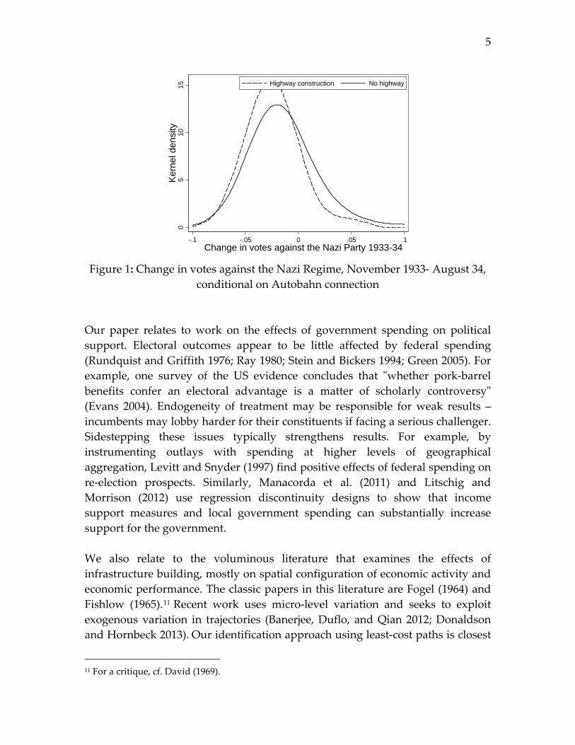
Figure 1 illustrates our main finding. It shows how much the building of the new
highways changed election results in each district, by plotting the distribution of
changes in the share of voters opposed to the Nazi regime between November
1933 and August 1934. There is a clear shift towards lower values – a faster
decline in opposition – for areas traversed by the new motorways. In an average
district, votes against the regime declined by 1.6 percentage points over this 9‐
month period (starting from already low levels).8 In precincts where the Autobahn
runs, the decline was 1.5‐times faster, amounting to an extra percentage point
reduction in opposition.9
In addition, we consider potential endogeneity problems – motorway planning
may have followed a political lead after 1933. To this end, we construct least‐cost
paths between terminal cities. These reflect the roughness of the terrain, the
number of rivers to be traversed, etc. We then use these least‐cost path as an
instrument for actual construction. The results suggest large effects of highway
construction even if we only focus on the part of the variation driven by
geographical characteristics.
What accounts for the Autobahn’s success in winning “hearts and minds”? We
discuss the economic and transport benefits. In the aggregate, these have been
shown to be minimal (Ritschl 1998; Vahrenkamp 2010). While these may have
played a role locally, we argue that the motorways also increased support
because they could be exploited by propaganda as powerful symbols of
competent, energetic government.10
7 In addition, building the Autobahn increased support for the Nazi regime country‐wide. Here,
we only identify the differential local effects. 8 Note that we use electoral results at the district level as our unit of observation. Nation‐wide,
the share of yes‐votes declined (with increases in many small districts and reductions in large
cities). 9 These results still hold if we control for a wide range of other variables and the selection of
precincts through which the highway ran, see Section 4. 10 This is in the spirit of Rogoff (1990).
5
05
10
15
Ker
nel d
ensi
ty
-.1 -.05 0 .05 .1Change in votes against the Nazi Party 1933-34
Highway construction No highway
Figure 1: Change in votes against the Nazi Regime, November 1933‐ August 34,
conditional on Autobahn connection
Our paper relates to work on the effects of government spending on political
support. Electoral outcomes appear to be little affected by federal spending
(Rundquist and Griffith 1976; Ray 1980; Stein and Bickers 1994; Green 2005). For
example, one survey of the US evidence concludes that ʺwhether pork‐barrel
benefits confer an electoral advantage is a matter of scholarly controversyʺ
(Evans 2004). Endogeneity of treatment may be responsible for weak results –
incumbents may lobby harder for their constituents if facing a serious challenger.
Sidestepping these issues typically strengthens results. For example, by
instrumenting outlays with spending at higher levels of geographical
aggregation, Levitt and Snyder (1997) find positive effects of federal spending on
re‐election prospects. Similarly, Manacorda et al. (2011) and Litschig and
Morrison (2012) use regression discontinuity designs to show that income
support measures and local government spending can substantially increase
support for the government.
We also relate to the voluminous literature that examines the effects of
infrastructure building, mostly on spatial configuration of economic activity and
economic performance. The classic papers in this literature are Fogel (1964) and
Fishlow (1965).11 Recent work uses micro‐level variation and seeks to exploit
exogenous variation in trajectories (Banerjee, Duflo, and Qian 2012; Donaldson
and Hornbeck 2013). Our identification approach using least‐cost paths is closest
11 For a critique, cf. David (1969).
6
in spirit to Faber (2014), who analyzes the effects of China’s national road
network construction on growth in areas that were not connected. Similar to
Donaldson (2014), we use information on earlier plans to add further credibility
to our identification exercise.
Relative to the existing literature, we make a number of contributions: First, we
show that infrastructure projects can turn opposition voters into supporters of
the regime. The fact that government spending can win over votes from the
opposition suggests that its effect must be substantial: in theory, changing voting
behavior will be harder the more remote voter’s tastes are from a given party’s
program (Lindbeck and Weibull, 1987). Second, while previous studies have
focused on elections in democracies, our results emerge in the context of a
nascent dictatorship: The construction of the German highway system helped to
entrench Hitler’s regime. We thus also contribute to a rich literature that studies
regime change in general and the rise of the Nazis in Germany more specifically
(King et al. 2008; Bracher 1978).
The paper proceeds as follows. We first explain the historical background and
context of motorway building in section II, and summarize key facts about
elections under the Nazi regime. We then describe our data in section III before
presenting our main empirical results (section IV). Next, we test the robustness of
our findings (section V). Section VI concludes.
II. Historical Background
In this section, we briefly describe motivations behind the building of the
Autobahn network and its antecedents. We also discuss the nature of early Nazi
elections and the growing strength of the regime.
Motorway building under the Nazis
The Hitler government pursued two aims with the building of the motorway
network. First, it aimed for a propaganda success, demonstrating its competence
by “getting things done”. This aim was pursued vigorously and with success –
many elderly Germans still point to the motorway network to argue that the
Nazi regime had some positive sides, too. Second, the government sought to
create employment.
7
The first sod of earth for building the Autobahn was turned by Adolf Hitler
himself, in September 1933. The weekly news reel shows him addressing a huge
crowd of workers, proclaiming that the “gigantic undertaking” was to bear
witness to the regime’s resolve and vision. He then told his audience to “get to
work”. Together with rearmament, the Autobahn is widely seen as a key part of
Keynesian demand‐stimulus by the Hitler government. In line with the regime’s
propaganda, many observers took it for granted that building the new highway
network reduced unemployment substantially. Quantitative research has since
established that neither military spending nor highway construction were
important in explaining Germany’s nascent recovery after 1933. Initially planned
to employ up to 600,000 workers, motorway building never came close to
creating such a number of jobs. At its peak, only 125,000 Germans were working
in highway construction. 12 Instead, the rapid rise in output under Hitler is
typically explained by the strength of a cyclical upswing, helped by an end to
deflation and declining uncertainty over the economy (Ritschl 1998).
Immediately after coming to power, the Nazi government began to push for new
road building projects. At the Berlin Motor Show – only 11 days after coming to
power – Hitler proposed far‐reaching plans on how to ‘motorize’ the German
people, providing not just roads but cheaper, compact cars. The new regime
could draw on earlier plans: Long before the Nazi government began to build
highways, a private think tank, the so‐called STUFA, developed detailed plans
for a comprehensive motorway network in Germany (Vahrenkamp 2010). In the
Rhineland, another – unrelated – project connected Bonn and Cologne. Konrad
Adenauer, later Chancellor of the Federal Republic of Germany, coordinated the
effort in a bid to reduce unemployment. It opened in 1932.14 By the summer of
1933, a new publicly‐owned company had been founded to build and operate the
new motorways. The network was planned with the help of a network of local
enthusiasts (Vahrenkamp 2010). The exact trajectory in several cases was decided
by Hitler himself, who insisted on scenic routes.
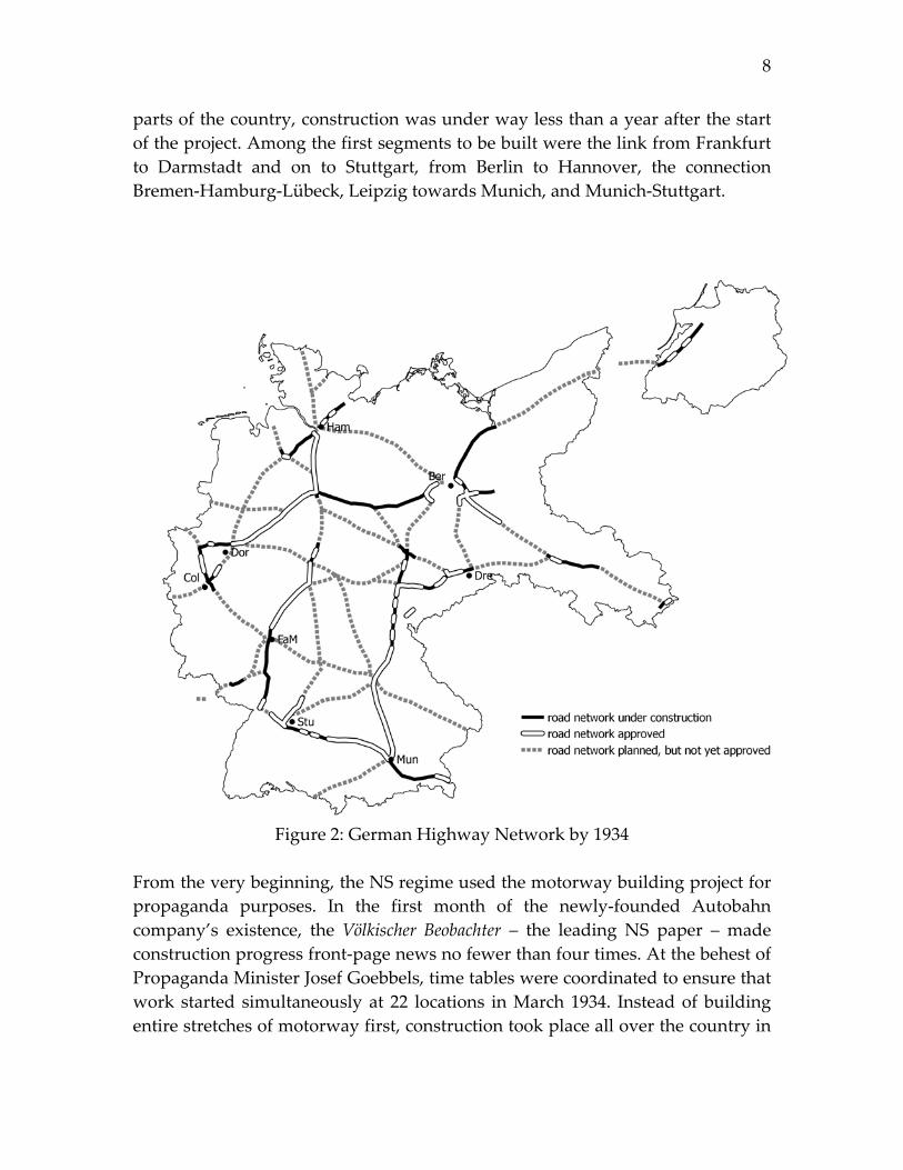
To maximize work creation and to demonstrate that the government was serious
about road building, construction began at many points simultaneously. Figure 2
shows the 1934 highway network. Black segments were under construction;
broad white segments were approved for construction, but not yet begun; and
dashed lines indicate planned segments not yet approved for construction. In 11
12 This should be compared with a decline in unemployment from 6 million in January 1933 to 2.5
million in the summer of 1934. 14 At the time, Italy had already completed the first high‐speed roads reserved for car traffic
8
parts of the country, construction was under way less than a year after the start
of the project. Among the first segments to be built were the link from Frankfurt
to Darmstadt and on to Stuttgart, from Berlin to Hannover, the connection
Bremen‐Hamburg‐Lübeck, Leipzig towards Munich, and Munich‐Stuttgart.
Figure 2: German Highway Network by 1934
From the very beginning, the NS regime used the motorway building project for
propaganda purposes. In the first month of the newly‐founded Autobahn
company’s existence, the Völkischer Beobachter – the leading NS paper – made
construction progress front‐page news no fewer than four times. At the behest of
Propaganda Minister Josef Goebbels, time tables were coordinated to ensure that
work started simultaneously at 22 locations in March 1934. Instead of building
entire stretches of motorway first, construction took place all over the country in
9
a bid to showcase NS economic policy. Speeches and news coverage emphasized
economic benefits, especially the reduction in unemployment.
As new stretches of motorway opened to the public, the regime celebrated its
successes. The first segment was finished in May 1935. Some 90,000 supporters
lined the road as Hitler was driven from Frankfurt to Darmstadt. By 1936, some
1,000 km of road (out of 9,000 planned) had been finished; the simultaneous
opening of 17 segments of motorway was used for ceremonies all over Germany.
Again, these events were used to high effect by the NS regime’s propaganda
machine. In addition, the Autobahn was also celebrated as an aesthetic innovation.
The Autobahn company commissioned a number of artists to produce paintings
of road segments, bridges, ramps, and construction work. A book containing
reproductions of these paintings sold over 50,000 copies.
Interestingly, motorway workers themselves were typically skeptical of the NS
regime – a fact that works against our finding. Recruited from the unemployed,
many were unskilled. A substantial share sympathized with the Social
Democratic Party or the Communist movement. While supporters of highway
construction had expected workers to be recruited locally, they were instead
often drafted from among the unemployed to work far from their homes, often
living in barracks, where they were subjected to harsh discipline, and received
only a minimal wage. They frequently expressed dissatisfaction with working
conditions, pay, and harsh discipline. Disaffected workers painted anti‐Nazi
slogans on lorries used for motorway construction (Evans 2006). In one incident,
workers demanded pay supplements. When their demands were not met, they
went on strike, singing “The International” – the anthem of the socialist and
communist workers’ movements. Work only resumed after the ringleaders were
sent to Dachau concentration camp.
The direct economic benefits of new roads were limited. Car ownership rates in
Germany in 1933 were low – approximately one quarter of those in England or
France. Most transport of goods and people took place via rail. The new regime
intended to boost the German car industry by all means possible, and not simply
via road‐building. Hitler had high hopes for the automobile industry as a future
source of employment, and because its factories could easily be converted to war
production. A tax exemption for the purchase of new automobiles from March
1933 onwards boosted car production, and accelerated the recovery of private car
purchases (which had begun to rise in the fall of 1932). Between 1932 and 1938,
the total number of cars, motorcycles and trucks on German roads doubled
(Evans 2006).
10
The military advantages of road‐building were relatively unimportant. While the
invasion of Austria used the Autobahn for moving tanks, almost all troop and
supply movements before and during World War II took place by rail. Since the
Hitler government planned wars of aggression which would take troops far
beyond the borders of the Reich, the importance of internal communications was
limited. If there was an aspect of road building that mattered militarily, it was
motor vehicle production. Boosting the mobility of army units was a general aim
of most armed forces after 1920. Increasing car ownership and the number of
trucks in Germany was considered desirable because private vehicles could be
confiscated in wartime. Indeed, the invasion of France used some 15,000 trucks
requisitioned from private industry (Vahrenkamp 2010).
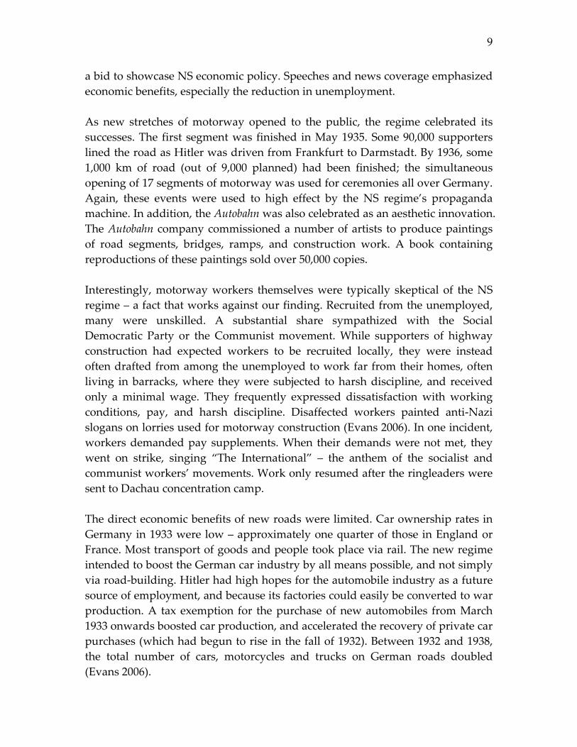
1933 Elections and the 1934 Plebiscite
We use two principal measures of opposition ‐‐ votes against the NSDAP in
November 1933, and the share of no‐votes in the plebiscite in 1934. In addition,
we use data from the March 1933 election for robustness checks, and to gauge
plausible magnitudes of actual vote shifts (since the later elections only provide
inflated measures of support) Figure 3 illustrates the timeline of elections and
highway building.
Figure 3: Timeline of events
When Germans went to the polls in March 1933, the Hitler government had
already been in power for over a month. Nonetheless, elections were still
relatively fair, with intimidation at the polls limited compared to what happened
on later occasions. Except for the Communist Party, which had been banned, all
parties that had competed during the last free election in November 1932 were
still on the ballot paper. Despite a massive propaganda campaign, the NSDAP
failed to win an absolute majority, receiving 44 percent of the total vote.
In November 1933, the regime held new elections. Over the summer, all parties
except the NSDAP had been banned. In addition to Nazi MPs, the NS list before
Last semi-free
elections
Highway planning. Breaking ground
in Sep ‘33
Election with NSDAP as the
only party.
Large-scale construction begins
in 131 counties.
19 Aug.1934 12 Nov.1933 Summer 1933 5 Mar.1933
Plebiscite granting vast
powers to Hitler
11
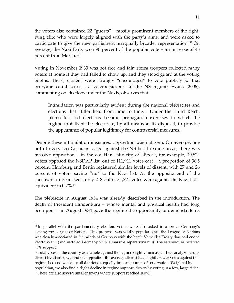
the voters also contained 22 “guests” – mostly prominent members of the right‐
wing elite who were largely aligned with the party’s aims, and were asked to
participate to give the new parliament marginally broader representation. 15 On
average, the Nazi Party won 90 percent of the popular vote – an increase of 48
percent from March.16
Voting in November 1933 was not free and fair; storm troopers collected many
voters at home if they had failed to show up, and they stood guard at the voting
booths. There, citizens were strongly “encouraged” to vote publicly so that
everyone could witness a voter’s support of the NS regime. Evans (2006),
commenting on elections under the Nazis, observes that
Intimidation was particularly evident during the national plebiscites and
elections that Hitler held from time to time… Under the Third Reich,
plebiscites and elections became propaganda exercises in which the
regime mobilized the electorate, by all means at its disposal, to provide
the appearance of popular legitimacy for controversial measures.
Despite these intimidation measures, opposition was not zero. On average, one
out of every ten Germans voted against the NS list. In some areas, there was
massive opposition – in the old Hanseatic city of Lübeck, for example, 40,824
voters opposed the NSDAP list, out of 111,911 votes cast – a proportion of 36.5
percent. Hamburg and Berlin registered similar levels of dissent, with 27 and 26
percent of voters saying ”no” to the Nazi list. At the opposite end of the
spectrum, in Pirmasens, only 218 out of 31,371 votes were against the Nazi list –
equivalent to 0.7%.17
The plebiscite in August 1934 was already described in the introduction. The
death of President Hindenburg – whose mental and physical health had long
been poor – in August 1934 gave the regime the opportunity to demonstrate its
15 In parallel with the parliamentary election, voters were also asked to approve Germany’s
leaving the League of Nations. This proposal was wildly popular since the League of Nations
was closely associated in the minds of Germans with the harsh Versailles Treaty that had ended
World War I (and saddled Germany with a massive reparations bill). The referendum received
95% support. 16 Total votes in the country as a whole against the regime slightly increased. If we analyze results
district by district, we find the opposite – the average district had slightly fewer votes against the
regime, because we count all districts as equally‐important units of observation. Weighted by
population, we also find a slight decline in regime support, driven by voting in a few, large cities. 17 There are also several smaller towns where support reached 100%.
12
popularity. The official union of the offices of President and Chancellor removed
the last de facto checks and balances that the Nazi state had inherited from the
Weimar constitution.
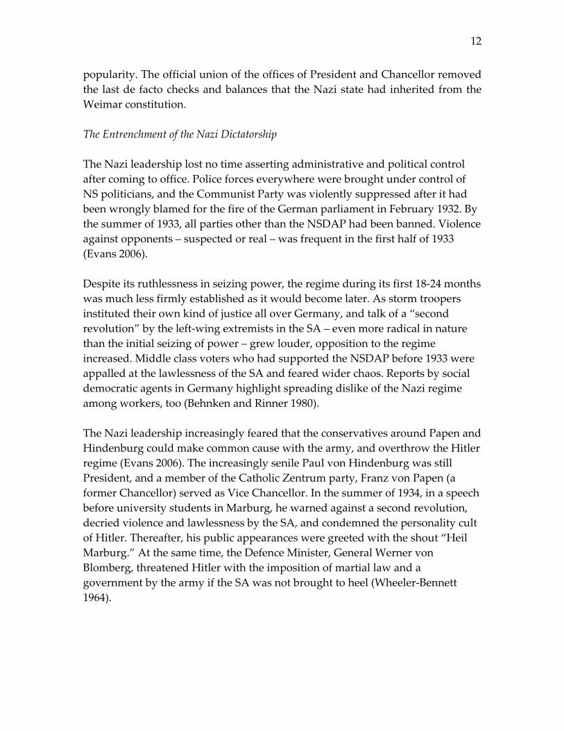
The Entrenchment of the Nazi Dictatorship
The Nazi leadership lost no time asserting administrative and political control
after coming to office. Police forces everywhere were brought under control of
NS politicians, and the Communist Party was violently suppressed after it had
been wrongly blamed for the fire of the German parliament in February 1932. By
the summer of 1933, all parties other than the NSDAP had been banned. Violence
against opponents – suspected or real – was frequent in the first half of 1933
(Evans 2006).
Despite its ruthlessness in seizing power, the regime during its first 18‐24 months
was much less firmly established as it would become later. As storm troopers
instituted their own kind of justice all over Germany, and talk of a “second
revolution” by the left‐wing extremists in the SA – even more radical in nature
than the initial seizing of power – grew louder, opposition to the regime
increased. Middle class voters who had supported the NSDAP before 1933 were
appalled at the lawlessness of the SA and feared wider chaos. Reports by social
democratic agents in Germany highlight spreading dislike of the Nazi regime
among workers, too (Behnken and Rinner 1980).
The Nazi leadership increasingly feared that the conservatives around Papen and
Hindenburg could make common cause with the army, and overthrow the Hitler
regime (Evans 2006). The increasingly senile Paul von Hindenburg was still
President, and a member of the Catholic Zentrum party, Franz von Papen (a
former Chancellor) served as Vice Chancellor. In the summer of 1934, in a speech
before university students in Marburg, he warned against a second revolution,
decried violence and lawlessness by the SA, and condemned the personality cult
of Hitler. Thereafter, his public appearances were greeted with the shout “Heil
Marburg.” At the same time, the Defence Minister, General Werner von
Blomberg, threatened Hitler with the imposition of martial law and a
government by the army if the SA was not brought to heel (Wheeler‐Bennett
1964).

13
The conflicts and threats of the summer of 1934 show that Nazi regime was still
very far from its omnipotent position at this stage, and that popular support
could by no means be taken for granted. It is for these reasons that the regime
tried hard to win “hearts and minds”, and why it cared about displays of
overwhelming popular support. It was only after the wholesale murder of the
SA‐leadership (plus several leading figures of the conservative opposition) in
1934, and after Hitler became both Chancellor and President, that the Nazi
regime became fully entrenched.
III. Data
We have voting records for 901 counties, covering the entire country. These data
are combined with information from the 1925 and 1933 censuses. To this, we add
geographical information from maps of the German road network in the
interwar period. We digitized separately the 1920s plans for the STUFA network,
and the various stages of expansion of the actual motorway network built after
the summer of 1933. In addition, we use information on pre‐existing transport
infrastructure in the form of rail and waterway links.
As shown in Table 1, of the 901 counties in our sample, 408 were scheduled to be
traversed by the Autobahn according to the general plan (shown in Figure 2),
while more than half – 493 – would not be touched by the new roads. Out of the
408 districts scheduled to be part of the network, there was construction by 1934
in 131 – roughly a third of the planned total.
Table 1: Number of Electoral Districts in Sample,
Conditional on Highway Construction
Part of
National
Highway
plan?
Highway under
construction in 1934
No Yes Total
No 493 0 493
Yes 277 131 408
Total 770 131 901
Since elections after 1933 were no longer fair and free, the support for the regime
as expressed at the polls surged. As the share of “yes” votes in many districts
approaches 100%, differences in the level of support naturally decline. Figure 4
plots the level of support in the three elections we analyze – the March 33
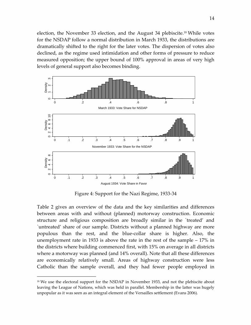
14
election, the November 33 election, and the August 34 plebiscite.18 While votes
for the NSDAP follow a normal distribution in March 1933, the distributions are
dramatically shifted to the right for the later votes. The dispersion of votes also
declined, as the regime used intimidation and other forms of pressure to reduce
measured opposition; the upper bound of 100% approval in areas of very high
levels of general support also becomes binding.
01
23
De
nsity
0 .2 .4 .6 .8 1
March 1933: Vote Share for NSDAP
02
46
810
De
nsity
0 .1 .2 .3 .4 .5 .6 .7 .8 .9 1
November 1933: Vote Share for the NSDAP
02
46
8D
ens
ity
0 .1 .2 .3 .4 .5 .6 .7 .8 .9 1
August 1934: Vote Share in Favor
Figure 4: Support for the Nazi Regime, 1933‐34
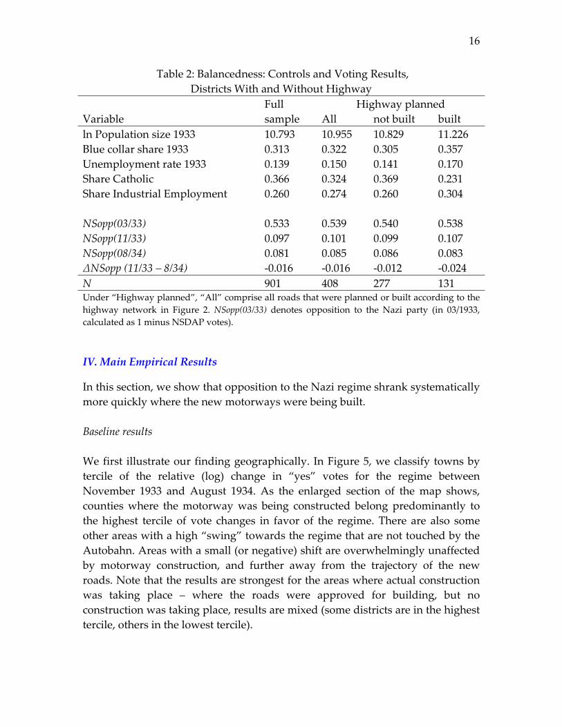
Table 2 gives an overview of the data and the key similarities and differences
between areas with and without (planned) motorway construction. Economic
structure and religious composition are broadly similar in the `treated’ and
`untreated’ share of our sample. Districts without a planned highway are more
populous than the rest, and the blue‐collar share is higher. Also, the
unemployment rate in 1933 is above the rate in the rest of the sample – 17% in
the districts where building commenced first, with 15% on average in all districts
where a motorway was planned (and 14% overall). Note that all these differences
are economically relatively small. Areas of highway construction were less
Catholic than the sample overall, and they had fewer people employed in
18 We use the electoral support for the NSDAP in November 1933, and not the plebiscite about
leaving the League of Nations, which was held in parallel. Membership in the latter was hugely
unpopular as it was seen as an integral element of the Versailles settlement (Evans 2006).
15
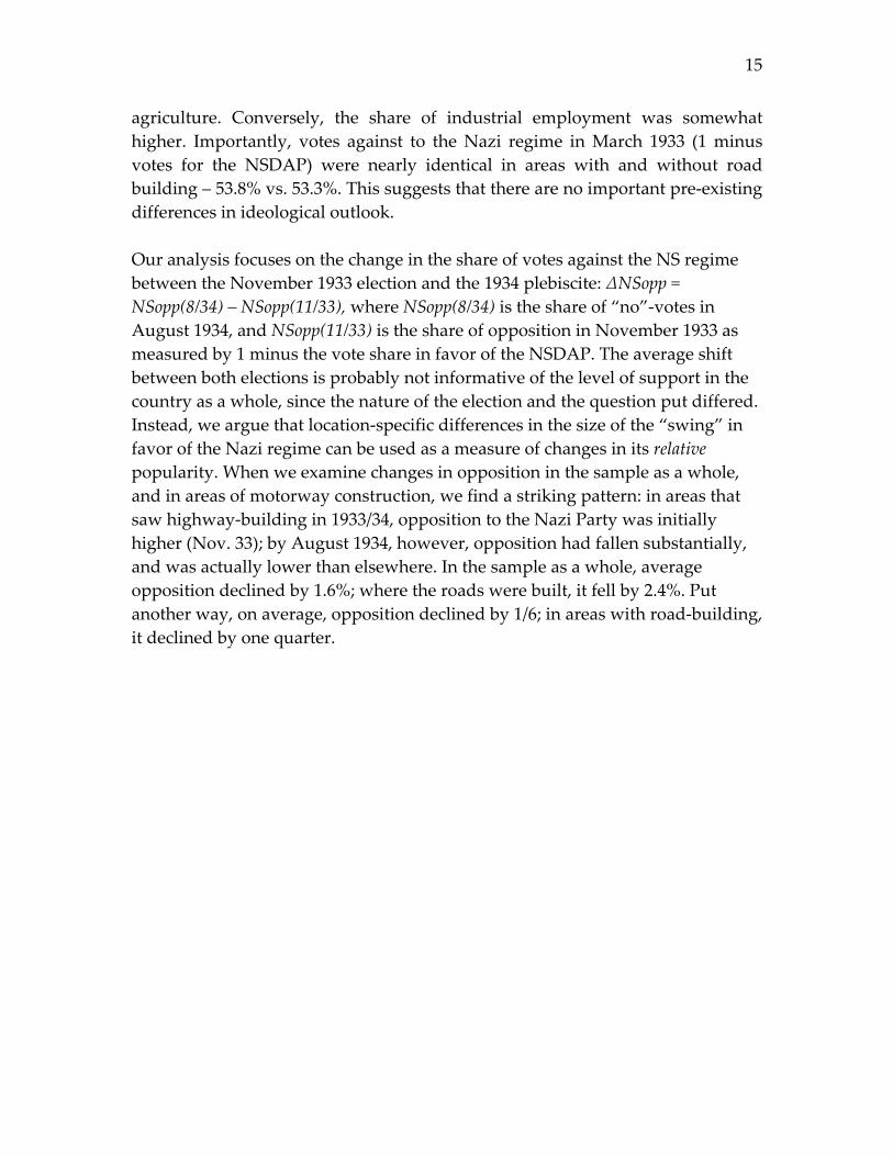
agriculture. Conversely, the share of industrial employment was somewhat
higher. Importantly, votes against to the Nazi regime in March 1933 (1 minus
votes for the NSDAP) were nearly identical in areas with and without road
building – 53.8% vs. 53.3%. This suggests that there are no important pre‐existing
differences in ideological outlook.
Our analysis focuses on the change in the share of votes against the NS regime
between the November 1933 election and the 1934 plebiscite: ∆NSopp =
NSopp(8/34) – NSopp(11/33), where NSopp(8/34) is the share of “no”‐votes in
August 1934, and NSopp(11/33) is the share of opposition in November 1933 as
measured by 1 minus the vote share in favor of the NSDAP. The average shift
between both elections is probably not informative of the level of support in the
country as a whole, since the nature of the election and the question put differed.
Instead, we argue that location‐specific differences in the size of the “swing” in
favor of the Nazi regime can be used as a measure of changes in its relative
popularity. When we examine changes in opposition in the sample as a whole,
and in areas of motorway construction, we find a striking pattern: in areas that
saw highway‐building in 1933/34, opposition to the Nazi Party was initially
higher (Nov. 33); by August 1934, however, opposition had fallen substantially,
and was actually lower than elsewhere. In the sample as a whole, average
opposition declined by 1.6%; where the roads were built, it fell by 2.4%. Put
another way, on average, opposition declined by 1/6; in areas with road‐building,
it declined by one quarter.
16
Table 2: Balancedness: Controls and Voting Results,
Districts With and Without Highway
Full Highway planned
Variable sample All not built built
ln Population size 1933 10.793 10.955 10.829 11.226
Blue collar share 1933 0.313 0.322 0.305 0.357
Unemployment rate 1933 0.139 0.150 0.141 0.170
Share Catholic 0.366 0.324 0.369 0.231
Share Industrial Employment 0.260 0.274 0.260 0.304
NSopp(03/33) 0.533 0.539 0.540 0.538
NSopp(11/33) 0.097 0.101 0.099 0.107
NSopp(08/34) 0.081 0.085 0.086 0.083
∆NSopp (11/33 – 8/34) ‐0.016 ‐0.016 ‐0.012 ‐0.024
N 901 408 277 131 Under “Highway planned”, “All” comprise all roads that were planned or built according to the
highway network in Figure 2. NSopp(03/33) denotes opposition to the Nazi party (in 03/1933,
calculated as 1 minus NSDAP votes).
IV. Main Empirical Results
In this section, we show that opposition to the Nazi regime shrank systematically
more quickly where the new motorways were being built.
Baseline results
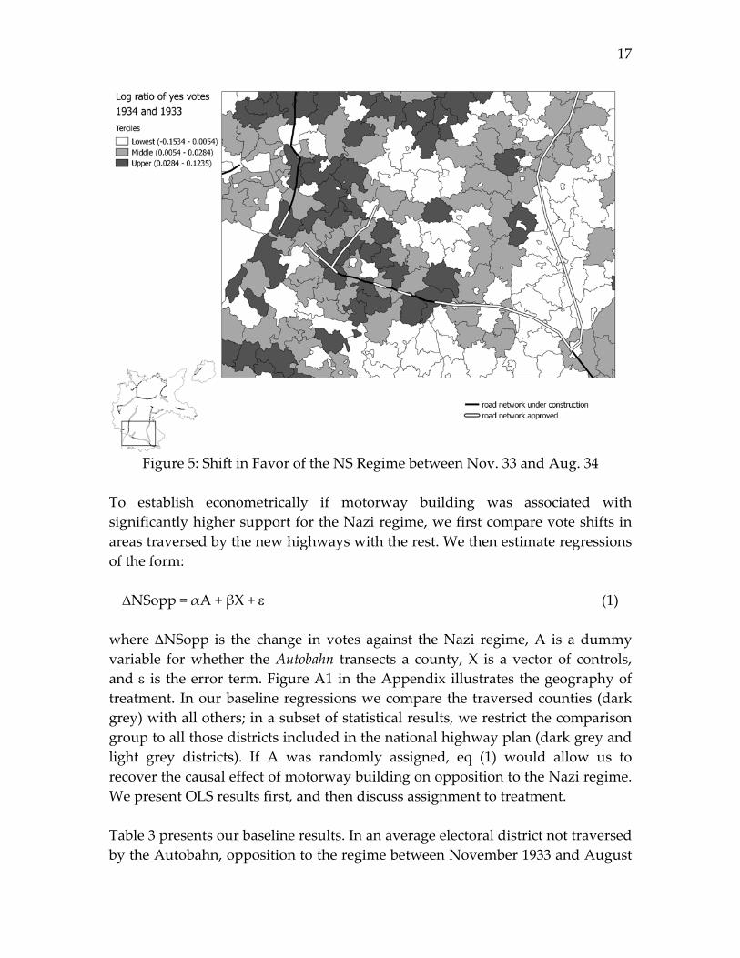
We first illustrate our finding geographically. In Figure 5, we classify towns by
tercile of the relative (log) change in “yes” votes for the regime between
November 1933 and August 1934. As the enlarged section of the map shows,
counties where the motorway was being constructed belong predominantly to
the highest tercile of vote changes in favor of the regime. There are also some
other areas with a high “swing” towards the regime that are not touched by the
Autobahn. Areas with a small (or negative) shift are overwhelmingly unaffected
by motorway construction, and further away from the trajectory of the new
roads. Note that the results are strongest for the areas where actual construction
was taking place – where the roads were approved for building, but no
construction was taking place, results are mixed (some districts are in the highest
tercile, others in the lowest tercile).
17
Figure 5: Shift in Favor of the NS Regime between Nov. 33 and Aug. 34
To establish econometrically if motorway building was associated with
significantly higher support for the Nazi regime, we first compare vote shifts in
areas traversed by the new highways with the rest. We then estimate regressions
of the form:
NSopp = αA + βX + (1)
where NSopp is the change in votes against the Nazi regime, A is a dummy
variable for whether the Autobahn transects a county, X is a vector of controls,
and is the error term. Figure A1 in the Appendix illustrates the geography of
treatment. In our baseline regressions we compare the traversed counties (dark
grey) with all others; in a subset of statistical results, we restrict the comparison
group to all those districts included in the national highway plan (dark grey and
light grey districts). If A was randomly assigned, eq (1) would allow us to
recover the causal effect of motorway building on opposition to the Nazi regime.
We present OLS results first, and then discuss assignment to treatment.
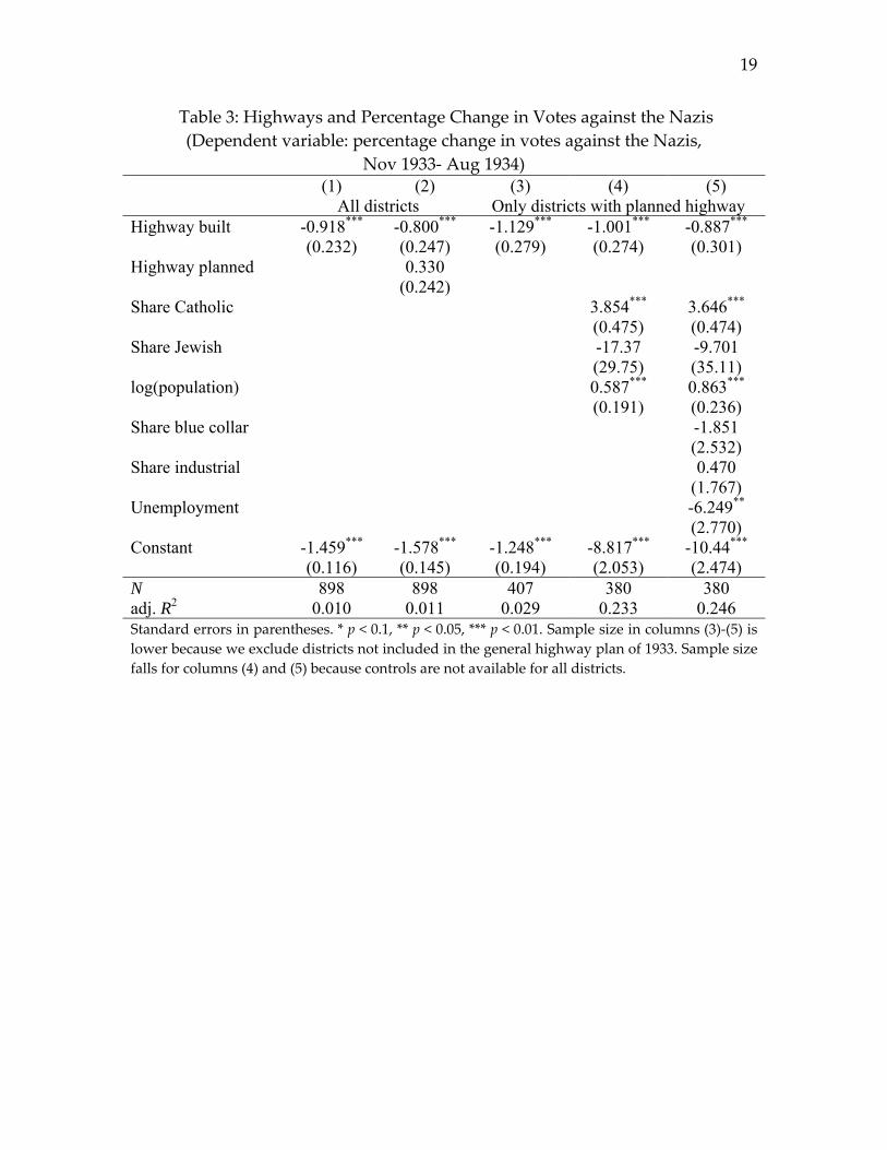
Table 3 presents our baseline results. In an average electoral district not traversed
by the Autobahn, opposition to the regime between November 1933 and August
18
1934 declined by 1.5 percentage points; where the new motorways were being
built, opposition declined by an additional 0.92 percentage points (col 1). In
relative terms, this is a large effect – highway building reduced opposition by an
additional 60 percent, relative to the baseline decline. In col 2, we add a dummy
variable for districts where highways – according to the general plan – were
going to be built in the future, but were not under construction in 1934. We find
no significant effect in districts where road‐building was merely planned. This
finding is important because it reduces the likelihood that some unobserved
factor that made road‐building feasible or desirable is responsible for the shift in
voting patterns.
In cols 3‐5, we focus on only those districts that were scheduled to become part
of the German highway network – roughly half of our sample. We also include
socioeconomic controls from the 1920s and 30s. The decline in opposition was
smaller in Catholic areas and in large cities, as implied by the positive
coefficients on these variables in cols 4 and 5. Where unemployment was high in
1933, opposition to the Nazis fell more strongly until August 1934 (col 5).
Industrial employment shares and the proportion of blue collar workers, on the
other hand, are not significantly associated with changes in opposition. In the
restricted sample in cols 3‐5, we find that building the Autobahn reduced
opposition by 0.85 to 1.1 percentage points. The result holds independent of the
socioeconomic characteristics that we add as controls. In terms of magnitude, the
effect of highway construction is substantial when compared to other
socioeconomic controls: a one standard deviation increase in Catholic population
raised opposition by 1.3 percentage points, and a one standard deviation increase
in initial unemployment lowered votes against the Nazis by 0.5 p.p. Below, we
discuss the size of these effects at greater length.
19
Table 3: Highways and Percentage Change in Votes against the Nazis
(Dependent variable: percentage change in votes against the Nazis,
Nov 1933‐ Aug 1934) (1) (2) (3) (4) (5) All districts Only districts with planned highway Highway built -0.918*** -0.800*** -1.129*** -1.001*** -0.887*** (0.232) (0.247) (0.279) (0.274) (0.301) Highway planned 0.330 (0.242) Share Catholic 3.854*** 3.646*** (0.475) (0.474) Share Jewish -17.37 -9.701 (29.75) (35.11) log(population) 0.587*** 0.863*** (0.191) (0.236) Share blue collar -1.851 (2.532) Share industrial 0.470 (1.767) Unemployment -6.249** (2.770) Constant -1.459*** -1.578*** -1.248*** -8.817*** -10.44*** (0.116) (0.145) (0.194) (2.053) (2.474) N 898 898 407 380 380 adj. R2 0.010 0.011 0.029 0.233 0.246 Standard errors in parentheses. * p < 0.1, ** p < 0.05, *** p < 0.01. Sample size in columns (3)‐(5) is
lower because we exclude districts not included in the general highway plan of 1933. Sample size
falls for columns (4) and (5) because controls are not available for all districts.
20
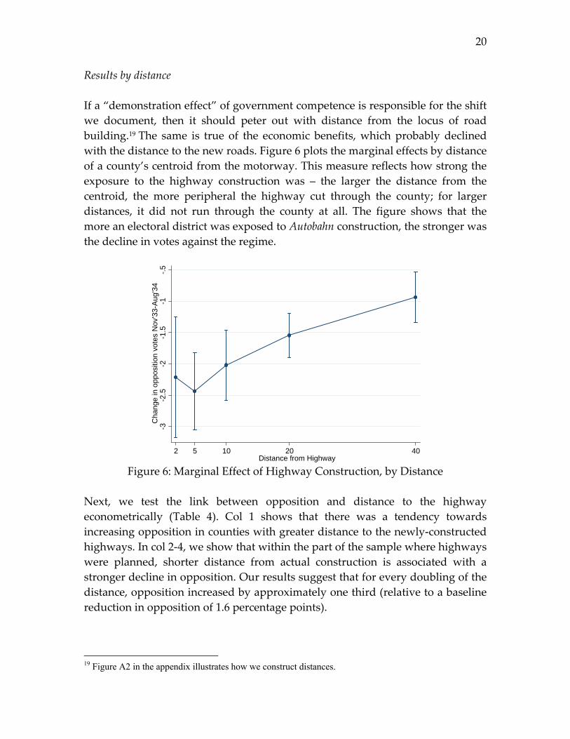
Results by distance
If a “demonstration effect” of government competence is responsible for the shift
we document, then it should peter out with distance from the locus of road
building.19 The same is true of the economic benefits, which probably declined
with the distance to the new roads. Figure 6 plots the marginal effects by distance
of a county’s centroid from the motorway. This measure reflects how strong the
exposure to the highway construction was – the larger the distance from the
centroid, the more peripheral the highway cut through the county; for larger
distances, it did not run through the county at all. The figure shows that the
more an electoral district was exposed to Autobahn construction, the stronger was
the decline in votes against the regime.
-3-2
.5-2
-1.5
-1-.
5C
hang
e in
opp
ositi
on v
otes
Nov
'33-
Aug
'34
2 5 10 20 40Distance from Highway
Figure 6: Marginal Effect of Highway Construction, by Distance
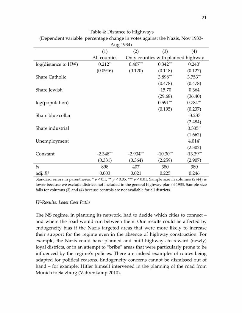
Next, we test the link between opposition and distance to the highway
econometrically (Table 4). Col 1 shows that there was a tendency towards
increasing opposition in counties with greater distance to the newly‐constructed
highways. In col 2‐4, we show that within the part of the sample where highways
were planned, shorter distance from actual construction is associated with a
stronger decline in opposition. Our results suggest that for every doubling of the
distance, opposition increased by approximately one third (relative to a baseline
reduction in opposition of 1.6 percentage points).
19 Figure A2 in the appendix illustrates how we construct distances.
21
Table 4: Distance to Highways
(Dependent variable: percentage change in votes against the Nazis, Nov 1933‐
Aug 1934)
(1) (2) (3) (4)
All counties Only counties with planned highway
log(distance to HW) 0.212** 0.407*** 0.342*** 0.240*
(0.0946) (0.120) (0.118) (0.127)
Share Catholic 3.898*** 3.753***
(0.478) (0.478)
Share Jewish ‐15.70 0.364
(29.68) (36.40)
log(population) 0.591*** 0.784***
(0.195) (0.237)
Share blue collar ‐3.237
(2.484)
Share industrial 3.335**
(1.662)
Unemployment 4.014*
(2.302)
Constant ‐2.348*** ‐2.904*** ‐10.30*** ‐13.39***
(0.331) (0.364) (2.259) (2.907)
N 898 407 380 380
adj. R2 0.003 0.021 0.225 0.246 Standard errors in parentheses. * p < 0.1, ** p < 0.05, *** p < 0.01. Sample size in columns (2)‐(4) is
lower because we exclude districts not included in the general highway plan of 1933. Sample size
falls for columns (3) and (4) because controls are not available for all districts.
IV‐Results: Least Cost Paths
The NS regime, in planning its network, had to decide which cities to connect –
and where the road would run between them. Our results could be affected by
endogeneity bias if the Nazis targeted areas that were more likely to increase
their support for the regime even in the absence of highway construction. For
example, the Nazis could have planned and built highways to reward (newly)
loyal districts, or in an attempt to “bribe” areas that were particularly prone to be
influenced by the regime’s policies. There are indeed examples of routes being
adapted for political reasons. Endogeneity concerns cannot be dismissed out of
hand – for example, Hitler himself intervened in the planning of the road from
Munich to Salzburg (Vahrenkamp 2010).
22
To avoid possible biases from roads being built to influence voters, or to reward
a pre‐existing shift towards the Nazis, we construct least‐cost paths for road
construction based on geographic characteristics. We then instrument actual
highway building with the least‐costs plans, and show that the variation in
building activity driven by the terrain predicts large declines in opposition to the
NS regime.21
Road construction is highly sensitive to the slope of the traversed terrain. We
calculate least‐cost paths to determine the cheapest way to connect cities that
appear in official German publications as terminal cities for the first wave of
highway construction.22 We then construct an indicator variable that takes on
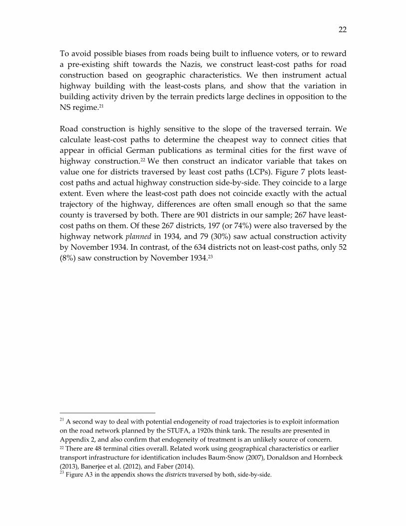
value one for districts traversed by least cost paths (LCPs). Figure 7 plots least‐
cost paths and actual highway construction side‐by‐side. They coincide to a large
extent. Even where the least‐cost path does not coincide exactly with the actual
trajectory of the highway, differences are often small enough so that the same
county is traversed by both. There are 901 districts in our sample; 267 have least‐
cost paths on them. Of these 267 districts, 197 (or 74%) were also traversed by the
highway network planned in 1934, and 79 (30%) saw actual construction activity
by November 1934. In contrast, of the 634 districts not on least‐cost paths, only 52
(8%) saw construction by November 1934.23
21 A second way to deal with potential endogeneity of road trajectories is to exploit information
on the road network planned by the STUFA, a 1920s think tank. The results are presented in
Appendix 2, and also confirm that endogeneity of treatment is an unlikely source of concern. 22 There are 48 terminal cities overall. Related work using geographical characteristics or earlier
transport infrastructure for identification includes Baum‐Snow (2007), Donaldson and Hornbeck
(2013), Banerjee et al. (2012), and Faber (2014). 23 Figure A3 in the appendix shows the districts traversed by both, side-by-side.
23
Figure 7: Least Costs Paths and Actual Highway Construction
(countries traversed highlighted)
Before presenting our IV results, we briefly discuss their interpretation.
Importantly, least cost paths affect the planning of highways, while the electoral
effects we are interested in are due to actual construction.24 In other words, least
cost paths affect voting via the planning of highways, which in turn translates
into highway construction in some districts – depending on the timing of
construction. The timing of construction, in turn, may still be endogenous.
Consequently, while we can address potential endogeneity in the location of
highways, we cannot do so for the timing of actual construction. Thus, we only
interpret the magnitude of the average effect of being located on a least cost path,
which is not affected by timing in the construction.
Table 5 presents our IV results. We present results using both planned highway
segments (odd columns) and actual construction (even columns). We also use
24 Cf. for example col 2 in Table 3, showing that only highway segments under construction, but
not those that were planned, drive our results.
24
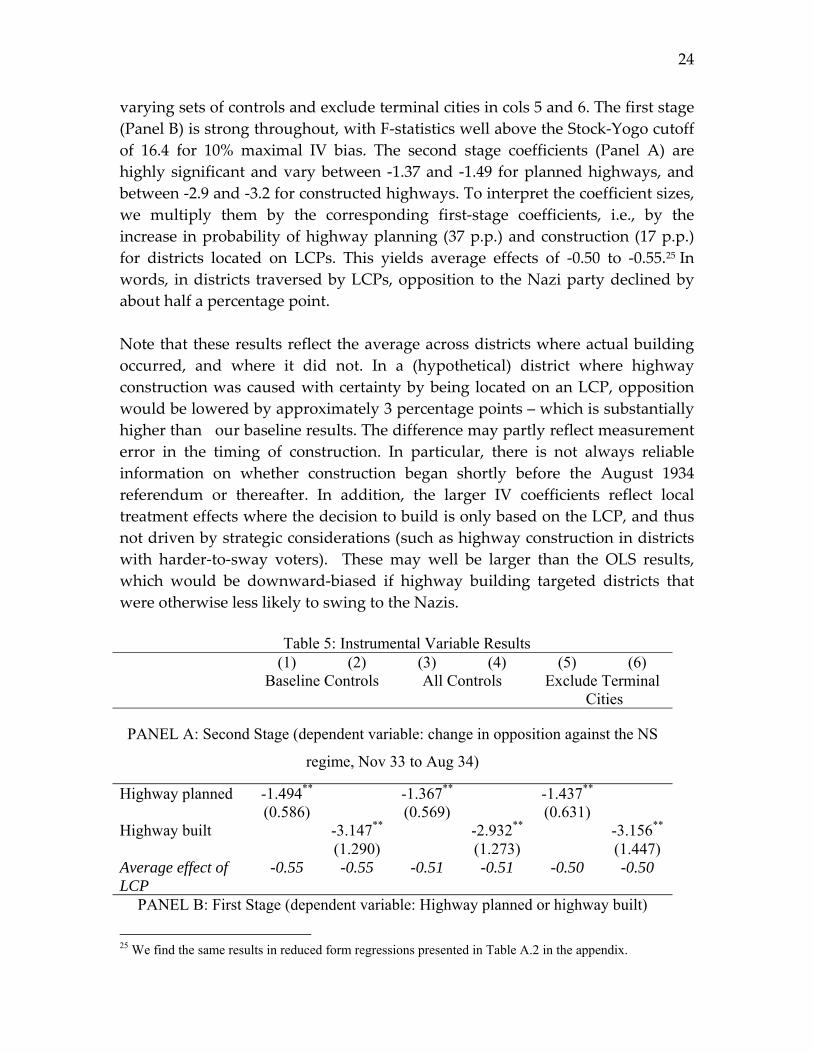
varying sets of controls and exclude terminal cities in cols 5 and 6. The first stage
(Panel B) is strong throughout, with F‐statistics well above the Stock‐Yogo cutoff
of 16.4 for 10% maximal IV bias. The second stage coefficients (Panel A) are
highly significant and vary between ‐1.37 and ‐1.49 for planned highways, and
between ‐2.9 and ‐3.2 for constructed highways. To interpret the coefficient sizes,
we multiply them by the corresponding first‐stage coefficients, i.e., by the
increase in probability of highway planning (37 p.p.) and construction (17 p.p.)
for districts located on LCPs. This yields average effects of ‐0.50 to ‐0.55.25 In
words, in districts traversed by LCPs, opposition to the Nazi party declined by
about half a percentage point.
Note that these results reflect the average across districts where actual building
occurred, and where it did not. In a (hypothetical) district where highway
construction was caused with certainty by being located on an LCP, opposition
would be lowered by approximately 3 percentage points – which is substantially
higher than our baseline results. The difference may partly reflect measurement
error in the timing of construction. In particular, there is not always reliable
information on whether construction began shortly before the August 1934
referendum or thereafter. In addition, the larger IV coefficients reflect local
treatment effects where the decision to build is only based on the LCP, and thus
not driven by strategic considerations (such as highway construction in districts
with harder‐to‐sway voters). These may well be larger than the OLS results,
which would be downward‐biased if highway building targeted districts that
were otherwise less likely to swing to the Nazis.
Table 5: Instrumental Variable Results
(1) (2) (3) (4) (5) (6) Baseline Controls All Controls Exclude Terminal
Cities
PANEL A: Second Stage (dependent variable: change in opposition against the NS
regime, Nov 33 to Aug 34)
Highway planned -1.494** -1.367** -1.437** (0.586) (0.569) (0.631) Highway built -3.147** -2.932** -3.156** (1.290) (1.273) (1.447) Average effect of LCP
-0.55 -0.55 -0.51 -0.51 -0.50 -0.50
PANEL B: First Stage (dependent variable: Highway planned or highway built)
25 We find the same results in reduced form regressions presented in Table A.2 in the appendix.
25
District on LCP 0.368*** 0.175*** 0.374*** 0.174*** 0.349*** 0.159*** (0.0361) (0.0307) (0.0358) (0.0304) (0.0382) (0.0316)F-Statistic 104.4 32.4 109.1 31.2 83.5 25.3 R2 0.149 0.116 0.156 0.138 0.115 0.111 [for both Panels:] BaselineControls Yes Yes Yes Yes Yes Yes AdditionalControls Yes Yes Yes Yes Observations 851 851 851 851 812 812 Standard errors in parentheses * p < 0.1, ** p < 0.05, *** p < 0.01. “LCP” is a dummy that takes on value one for counties cut by the Least Cost Path of construction that connects two terminal cities. BaselineControls include share Catholic, share of Jews (both in 1925), and log of population in 1933. AdditionalControls include the share of blue collar workers, the share of agricultural and industrial employment, and unemployment (all in 1933).
V. Robustness and Discussion
In this section, we discuss the possibility of differential intimidation driving our
results, and we show that our results hold across a wide range of subsamples.
We also present results from a number of placebo tests, use matching estimation,
and present an analysis of voting results in levels. The latter addresses the
question whether highways were built where electoral support for the Nazis was
already strong. Finally, we investigate the possibility of electoral fraud.
Differential voter intimidation
One obvious concern with our data is that (changes in) votes for the opposition
do not reflect genuine changes in preferences, but instead capture differential
increases in the regime’s repressive activities. In particular – given that public
officials were under pressure to show that “their” districts supported the regime
– it is entirely possible that districts with highway construction saw greater levels
of intimidation at the polling station.
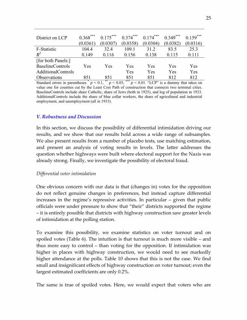
To examine this possibility, we examine statistics on voter turnout and on
spoiled votes (Table 6). The intuition is that turnout is much more visible – and
thus more easy to control – than voting for the opposition. If intimidation was
higher in places with highway construction, we would need to see markedly
higher attendance at the polls. Table 10 shows that this is not the case. We find
small and insignificant effects of highway construction on voter turnout; even the
largest estimated coefficients are only 0.2%.
The same is true of spoiled votes. Here, we would expect that voters who are
26
afraid ‐ because votes against the regime might be monitored and could lead to
repression – would be more likely to register their opposition by spoiling their
ballot papers instead, since this could always be construed as an honest mistake.
This is not what we find. Where the highways ran or were built, voters were
overall less likely to spoil their votes. The effect is insignificant in all
specifications except for col (8). In combination, these results suggest that there is
no reason to think that differential repression is a likely driver of our results.
Table 6: Election Turnout and Spoiled Votes
(1) (2) (3) (4) (5) (6) (7) (8)
Turnout 11/33 Turnout 8/34 Spoiled 11/33 Spoiled 8/34
Sample All HW‡ All HW‡ All HW‡ All HW‡
HW 0.194 0.0531 0.209 0.0626 -0.231 -0.522 -0.123 -0.174**
built (0.176) (0.187) (0.170) (0.177) (0.270) (0.323) (0.0790) (0.0869)
Controls yes yes yes yes yes yes yes yes
N 851 380 851 380 851 380 851 380
adj. R2 0.138 0.240 0.132 0.233 0.338 0.382 0.252 0.192Dependent variable is election turnout (max. 100) in cols 1‐4, and spoiled votes (defined as
100×invalid votes/votes cast) in cols 5‐8. Standard errors in parentheses. * p < 0.1, ** p < 0.05, *** p
< 0.01. Controls are the same as those used in Table 3. ‡Districts with planned highway construction
Sample splits
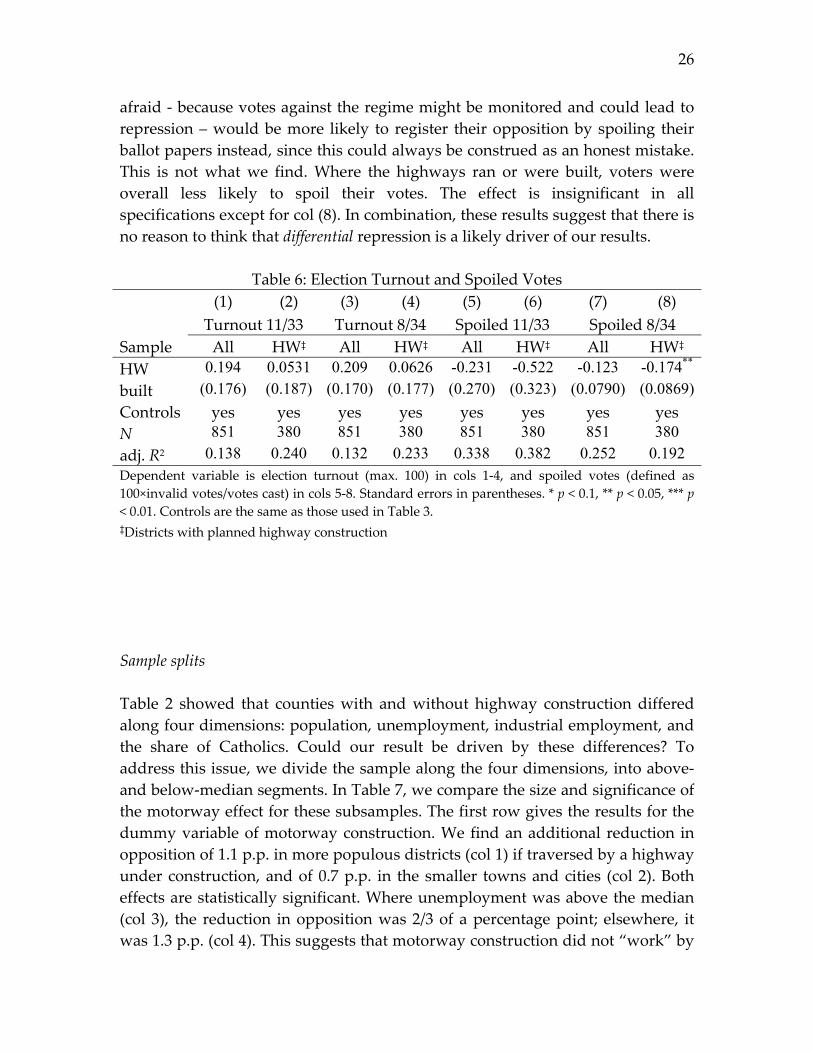
Table 2 showed that counties with and without highway construction differed
along four dimensions: population, unemployment, industrial employment, and
the share of Catholics. Could our result be driven by these differences? To
address this issue, we divide the sample along the four dimensions, into above‐
and below‐median segments. In Table 7, we compare the size and significance of
the motorway effect for these subsamples. The first row gives the results for the
dummy variable of motorway construction. We find an additional reduction in
opposition of 1.1 p.p. in more populous districts (col 1) if traversed by a highway
under construction, and of 0.7 p.p. in the smaller towns and cities (col 2). Both
effects are statistically significant. Where unemployment was above the median
(col 3), the reduction in opposition was 2/3 of a percentage point; elsewhere, it
was 1.3 p.p. (col 4). This suggests that motorway construction did not “work” by
27
targeting depressed areas and offering support for the unemployed. Along
similar lines, higher industrial employment is also associated with smaller
reductions in opposition. Finally, the highway construction is associated with a
reduction in opposition in both Catholic and Protestant counties (cols 7,8). The
effect is somewhat smaller in pre‐dominantly Protestant areas, where the Nazi
party received higher levels of support during its rise to power (Falter 1991). The
stronger effect in Catholic areas suggests that highway construction was
particularly powerful in overcoming opposition in areas that had earlier been
less receptive to the Nazi program and propaganda.
Table 7: Sample Splits
(1) (2) (3) (4) (5) (6) (7) (8)
Population Unemployment Industry Emp. Share Catholic
Rel. to
median
Above Below Above Below Above Below Above Below
HW
built
‐1.130*** ‐0.742* ‐0.667* ‐1.274*** ‐
0.675**
‐
1.230***
‐
1.816***
‐0.479*
(0.343) (0.426) (0.343) (0.413) (0.341) (0.464) (0.546) (0.250)
HW
planned
0.947*** 0.342 0.359 0.849*** 0.294 0.857*** 0.635* 0.570**
(0.335) (0.277) (0.310) (0.313) (0.329) (0.292) (0.358) (0.231)
Baseline
Controls
yes yes yes yes yes yes yes yes
N 420 431 427 424 427 424 431 420
adj. R2 0.319 0.135 0.174 0.246 0.175 0.218 0.074 0.007 Standard errors in parentheses. * p < 0.1, ** p < 0.05, *** p < 0.01. Baseline controls include the share
of Catholics, share of Jews (both in 1925), and log county population in 1933.
Earlier electoral support for the NSDAP and road‐building
Next, we examine the relationship between road‐building and (i) NSDAP votes
in March 1933, and (ii) the change in votes against the NSDAP between March
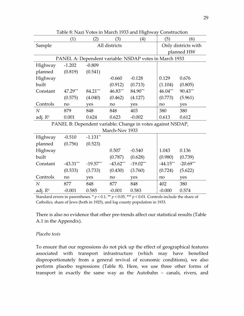
and November. Table 8 gives the results. In Panel A we find that there is no
significant association between election results in March 1933 and inclusion in
the planned highway network (cols 1‐2); nor is the actual building of the
Autobahn associated with the NSDAP’s electoral success in the last semi‐free
election in March 1933 (cols 3‐6). If we restrict the analysis to areas included in
the 1934 plan, we find small and insignificant positive coefficients. Overall, votes
28
for NSDAP in March 1933 in districts with future Autobahn construction were
statistically indistinguishable from the rest.
In Panel B we analyze the decline in votes against the Nazis between March and
November 1933, i.e., before most of the building had started, but when the routes
were known. Overall, votes against the NSDAP fell by 43 p.p. – from 53% to
10%.27 Our results in cols 1 and 2 suggest that this decline in opposition was
marginally stronger in counties that were included in the Reich’s Autobahn‐
network. This suggests that anticipated building had a (limited) effect on votes in
the expected direction. However, highway building itself did not change
opposition to the Nazis between March and November 1933. This is close to a
placebo check of our results: because actual building began in earnest after the
fall of 1933, we should expect small or no effects of building on votes.
27 As we mentioned above, the levels of the two election results cannot be readily compared.
However, the differential decline of opposition in the cross‐section is probably informative of the
relative changes in support in different counties.
29
Table 8: Nazi Votes in March 1933 and Highway Construction
(1) (2) (3) (4) (5) (6)
Sample All districts Only districts with
planned HW
PANEL A: Dependent variable: NSDAP votes in March 1933
Highway ‐1.202 ‐0.809
planned (0.819) (0.541)
Highway ‐0.660 ‐0.128 0.129 0.676
built (0.912) (0.713) (1.104) (0.805)
Constant 47.29*** 84.21*** 46.83*** 84.90*** 46.04*** 90.43***
(0.575) (4.040) (0.462) (4.127) (0.773) (5.961)
Controls no yes no yes no yes
N 879 848 848 403 380 380
adj. R2 0.001 0.624 0.623 ‐0.002 0.613 0.612
PANEL B: Dependent variable: Change in votes against NSDAP,
March‐Nov 1933
Highway ‐0.510 ‐1.131**
planned (0.756) (0.523)
Highway 0.507 ‐0.540 1.043 0.136
built (0.787) (0.628) (0.980) (0.739)
Constant ‐43.31*** ‐19.57*** ‐43.62*** ‐19.02*** ‐44.15*** ‐20.69***
(0.533) (3.733) (0.430) (3.760) (0.724) (5.622)
Controls no yes no yes no yes
N 877 848 877 848 402 380
adj. R2 ‐0.001 0.585 ‐0.001 0.583 ‐0.000 0.574 Standard errors in parentheses. * p < 0.1, ** p < 0.05, *** p < 0.01. Controls include the share of
Catholics, share of Jews (both in 1925), and log county population in 1933.
There is also no evidence that other pre‐trends affect our statistical results (Table
A.1 in the Appendix).
Placebo tests
To ensure that our regressions do not pick up the effect of geographical features
associated with transport infrastructure (which may have benefited
disproportionately from a general revival of economic conditions), we also
perform placebo regressions (Table 8). Here, we use three other forms of
transport in exactly the same way as the Autobahn – canals, rivers, and
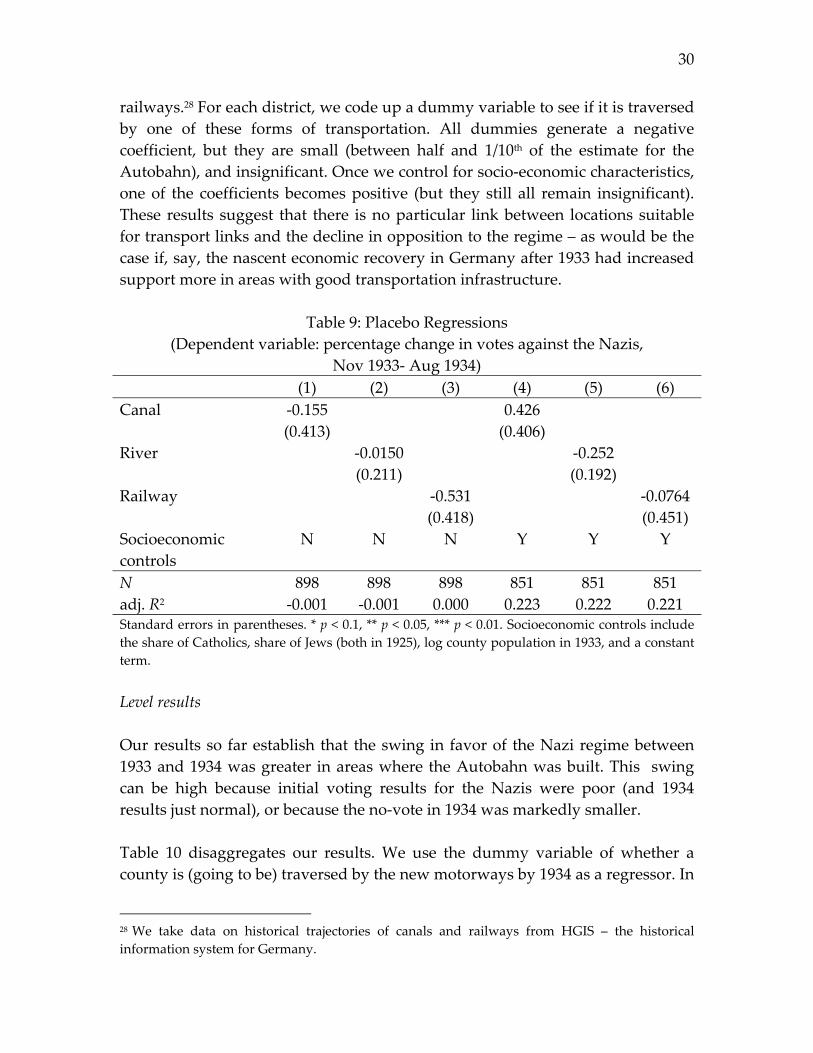
30
railways.28 For each district, we code up a dummy variable to see if it is traversed
by one of these forms of transportation. All dummies generate a negative
coefficient, but they are small (between half and 1/10th of the estimate for the
Autobahn), and insignificant. Once we control for socio‐economic characteristics,
one of the coefficients becomes positive (but they still all remain insignificant).
These results suggest that there is no particular link between locations suitable
for transport links and the decline in opposition to the regime – as would be the
case if, say, the nascent economic recovery in Germany after 1933 had increased
support more in areas with good transportation infrastructure.
Table 9: Placebo Regressions
(Dependent variable: percentage change in votes against the Nazis,
Nov 1933‐ Aug 1934)
(1) (2) (3) (4) (5) (6)
Canal ‐0.155 0.426
(0.413) (0.406)
River ‐0.0150 ‐0.252
(0.211) (0.192)
Railway ‐0.531 ‐0.0764
(0.418) (0.451)
Socioeconomic
controls
N N N Y Y Y
N 898 898 898 851 851 851
adj. R2 ‐0.001 ‐0.001 0.000 0.223 0.222 0.221 Standard errors in parentheses. * p < 0.1, ** p < 0.05, *** p < 0.01. Socioeconomic controls include
the share of Catholics, share of Jews (both in 1925), log county population in 1933, and a constant
term.
Level results
Our results so far establish that the swing in favor of the Nazi regime between
1933 and 1934 was greater in areas where the Autobahn was built. This swing
can be high because initial voting results for the Nazis were poor (and 1934
results just normal), or because the no‐vote in 1934 was markedly smaller.
Table 10 disaggregates our results. We use the dummy variable of whether a
county is (going to be) traversed by the new motorways by 1934 as a regressor. In
28 We take data on historical trajectories of canals and railways from HGIS – the historical
information system for Germany.
31
col 1, we examine if these areas saw a higher level of opposition in 1933. The
coefficient on whether a county sees road building is small and positive, but
insignificant (in line with results in Table 7). This suggests that (non‐)Nazi votes
did not differ in areas that would see the construction of highways a year later.
Beginning in col 2, we use votes against the Nazis in August 1934 as dependent
variable. For this election, which occurred after highway building had started,
we find a significantly lower level of opposition. This is also true if we control for
the level of votes against the Nazis in March 1933 (col 3). Also, the positive
coefficient on votes against the Nazis in March 1933 implies that local opposition
is persistent – areas that opposed the Nazi in March 1933 did so again in 1934 to
a significant extent. In col 4, we add information on motorways planned, but not
yet built. These themselves do not create significant shifts in levels, but they also
do not affect the size or significance of our main finding. Finally, in col 5 we
control for the vote shares for other parties in March 1933 – the Communists, the
Social Democrats, and the Centre Party. Our main result is unchanged – highway
building led to a significant reduction in opposition to the NS regime between
November 1933 and August 1934.
32
Table 10: Level of Votes Against the Nazi Regime and Highway Construction
Dep. Var.: Share of “no” votes in August 1934
(1) (2) (3) (4) (5)
Dep. Var. non‐NSDAP
03/33
“no“
08/34
“no“
08/34
“no“
08/34
“no“
08/34
Highway built 0.128 ‐0.867** ‐0.896** ‐0.849** ‐0.825**
(0.770) (0.382) (0.349) (0.359) (0.375)
non‐NSDAP 03/33 16.10*** 16.06***
(1.766) (1.765)
Road planned 0.118
(0.295)
Socioeconomic
controls
Y Y Y Y Y
Other party vote
shares*
N N N N Y
N 848 851 848 848 848
adj. R2 0.623 0.311 0.381 0.381 0.349 * Other parties include the votes shares in March 1933 for the Communist Party (KPD), the
Centre Party (Zentrum), and the Social Democratic Party (SPD). non‐NSDAP 03/33 is 1‐voteshare
of the NSDAP in the March 1933 election; “no“ 08/34 is the share of no‐votes in the August 1934
plebiscite.
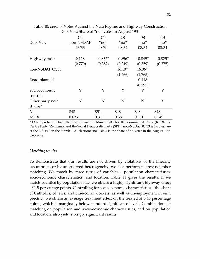
Matching results
To demonstrate that our results are not driven by violations of the linearity
assumption, or by unobserved heterogeneity, we also perform nearest‐neighbor
matching. We match by three types of variables – population characteristics,
socio‐economic characteristics, and location. Table 11 gives the results. If we
match counties by population size, we obtain a highly significant highway effect
of 1.5 percentage points. Controlling for socioeconomic characteristics – the share
of Catholics, of Jews, and blue‐collar workers, as well as unemployment in each
precinct, we obtain an average treatment effect on the treated of 0.43 percentage
points, which is marginally below standard significance levels. Combinations of
matching on population and socio‐economic characteristics, and on population
and location, also yield strongly significant results.
33
Table 11: Matching Results
matching variables SATT Z‐score p‐value
Population ‐1.454 3.55 0.0001
Socio‐economic ‐0.43 1.61 0.107
Population + socio‐economic ‐0.52 2.08 0.038
Population + location ‐0.76 2.83 0.005 Note: SATT – treatment effect for the treated. We use the nnmatch routine from Abadie et al.
(2004), with nearest neighbor matching for the three nearest matches. Matching on location is
based on the latitude and longitude of the centroid of each county.
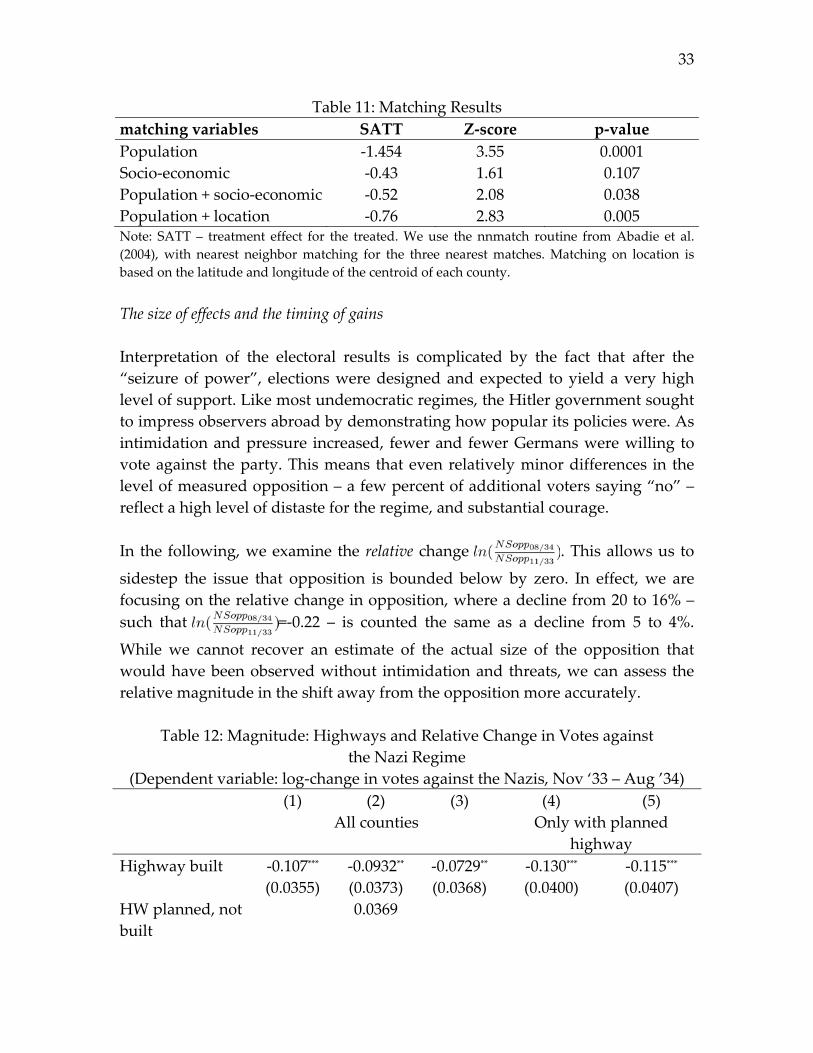
The size of effects and the timing of gains
Interpretation of the electoral results is complicated by the fact that after the
“seizure of power”, elections were designed and expected to yield a very high
level of support. Like most undemocratic regimes, the Hitler government sought
to impress observers abroad by demonstrating how popular its policies were. As
intimidation and pressure increased, fewer and fewer Germans were willing to
vote against the party. This means that even relatively minor differences in the
level of measured opposition – a few percent of additional voters saying “no” –
reflect a high level of distaste for the regime, and substantial courage.
In the following, we examine the relative change . This allows us to
sidestep the issue that opposition is bounded below by zero. In effect, we are
focusing on the relative change in opposition, where a decline from 20 to 16% –
such that =‐0.22 – is counted the same as a decline from 5 to 4%.
While we cannot recover an estimate of the actual size of the opposition that
would have been observed without intimidation and threats, we can assess the
relative magnitude in the shift away from the opposition more accurately.
Table 12: Magnitude: Highways and Relative Change in Votes against
the Nazi Regime
(Dependent variable: log‐change in votes against the Nazis, Nov ‘33 – Aug ’34)
(1) (2) (3) (4) (5)
All counties Only with planned
highway
Highway built ‐0.107*** ‐0.0932** ‐0.0729** ‐0.130*** ‐0.115***
(0.0355) (0.0373) (0.0368) (0.0400) (0.0407)
HW planned, not
built
0.0369
34
(0.0296)
Controls Yes Yes
Constant ‐0.238*** ‐0.251*** ‐1.123*** ‐0.214*** ‐1.666***
(0.0144) (0.0183) (0.216) (0.0232) (0.283)
N 898 898 851 407 380
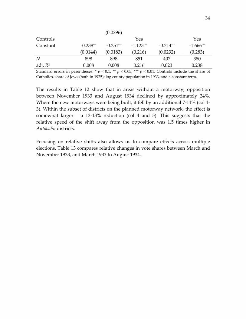
adj. R2 0.008 0.008 0.216 0.023 0.238 Standard errors in parentheses. * p < 0.1, ** p < 0.05, *** p < 0.01. Controls include the share of
Catholics, share of Jews (both in 1925); log county population in 1933, and a constant term.
The results in Table 12 show that in areas without a motorway, opposition
between November 1933 and August 1934 declined by approximately 24%.
Where the new motorways were being built, it fell by an additional 7‐11% (col 1‐
3). Within the subset of districts on the planned motorway network, the effect is
somewhat larger – a 12‐13% reduction (col 4 and 5). This suggests that the
relative speed of the shift away from the opposition was 1.5 times higher in
Autobahn districts.
Focusing on relative shifts also allows us to compare effects across multiple
elections. Table 13 compares relative changes in vote shares between March and
November 1933, and March 1933 to August 1934.
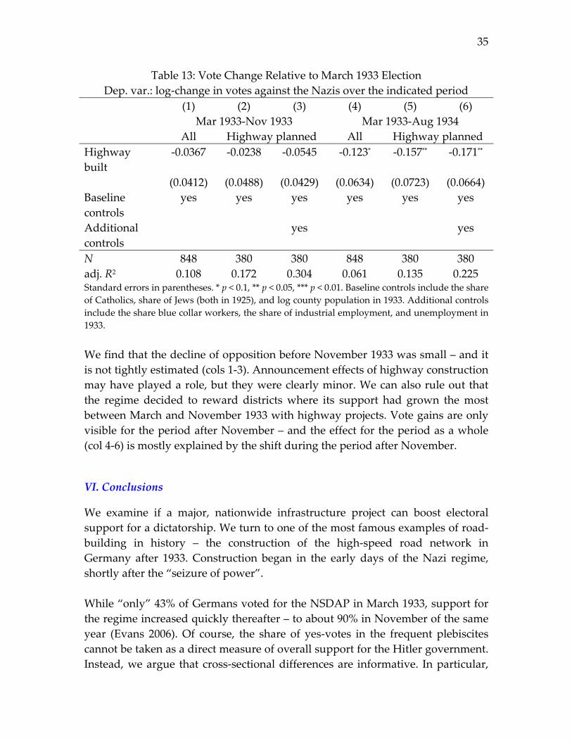
35
Table 13: Vote Change Relative to March 1933 Election
Dep. var.: log‐change in votes against the Nazis over the indicated period
(1) (2) (3) (4) (5) (6)
Mar 1933‐Nov 1933 Mar 1933‐Aug 1934
All Highway planned All Highway planned
Highway
built
‐0.0367 ‐0.0238 ‐0.0545 ‐0.123* ‐0.157** ‐0.171**
(0.0412) (0.0488) (0.0429) (0.0634) (0.0723) (0.0664)
Baseline
controls
yes yes yes yes yes yes
Additional
controls
yes yes
N 848 380 380 848 380 380
adj. R2 0.108 0.172 0.304 0.061 0.135 0.225 Standard errors in parentheses. * p < 0.1, ** p < 0.05, *** p < 0.01. Baseline controls include the share
of Catholics, share of Jews (both in 1925), and log county population in 1933. Additional controls
include the share blue collar workers, the share of industrial employment, and unemployment in
1933.
We find that the decline of opposition before November 1933 was small – and it
is not tightly estimated (cols 1‐3). Announcement effects of highway construction
may have played a role, but they were clearly minor. We can also rule out that
the regime decided to reward districts where its support had grown the most
between March and November 1933 with highway projects. Vote gains are only
visible for the period after November – and the effect for the period as a whole
(col 4‐6) is mostly explained by the shift during the period after November.
VI. Conclusions
We examine if a major, nationwide infrastructure project can boost electoral
support for a dictatorship. We turn to one of the most famous examples of road‐
building in history – the construction of the high‐speed road network in
Germany after 1933. Construction began in the early days of the Nazi regime,
shortly after the “seizure of power”.
While “only” 43% of Germans voted for the NSDAP in March 1933, support for
the regime increased quickly thereafter – to about 90% in November of the same
year (Evans 2006). Of course, the share of yes‐votes in the frequent plebiscites
cannot be taken as a direct measure of overall support for the Hitler government.
Instead, we argue that cross‐sectional differences are informative. In particular,
36
we examine the size of the electoral swing in favor of the regime during a
relatively short period of time – between November 1933 and August 1934.
While the layout of the road network was largely determined by the fall of 1933,
spending on road building only reached significant levels by the spring of 1934.
We find that electoral opposition to the nascent dictatorship declined
significantly in districts traversed by the Autobahn. This effect is much bigger
after November 1933 than before, in line with spending patterns over time. There
is a clear gradient to the collapse in opposition – the further away from the
highways a district was, the smaller the reduction in opposition.
The effects are both large and likely to be causal. We find that the decline in
opposition was about 50% faster in districts with an Autobahn connection than in
the rest. By comparing changes in districts that would have been traversed by the
motorways planned in 1926 with those in areas that actually saw construction,
we also establish that roads added or altered by the Nazi planners are not
responsible for the additional vote shifts we document – the decline in
opposition was identical in Autobahn districts included in early plans and those
added after 1933. This rules out that the revised 1933 plans “chased” growing
support in some districts.
Why did motorway building reduce opposition to the regime? We cannot
directly establish the channels through which the Autobahn helped to win the
“hearts and minds” of Germans. The Nazi regime prioritized road‐building as
an economic stimulus measure. Original plans were for 600,000 workers to be
employed; the actual maximum was 125,000. Recent analysis suggests that
economic effects in the aggregate were modest (Ritschl 1998). The benefits in
terms of transport were also minimal – Germany had one of the lowest rates of
car ownership in Europe (Evans 2006).
Nonetheless, it is possible that local effects were much larger. Workers were
initially housed in private homes in the villages and towns where the roads were
being built; barracks were only built later. Those employed in building the road
also spent money in inns and shops; construction crews organized film showings,
and construction sites became minor local attractions – a popular destination for
weekend trips (Eichner‐Ramm 2008).
An alternative channel is that the Autobahn demonstrated the new government’s
determination and competence in a convincing fashion. Voters may have
perceived motorway construction as a sign of “competence”, along the lines of
Rogoff (1990). Similarly, the Autobahn served as a convincing proof of Nazi
37
Germany’s ability to get things done – a project to showcase the ruthless energy
and organizational capabilities of the new regime, as Hitler promised in his
speech inaugurating the project. Emphasized as a key factor for economic revival,
the rapid fall in unemployment after 1933 convinced many that road‐building
had “worked”. After the perceived incompetence and gridlock of Weimar
politics, many Germans were undoubtedly impressed by the rapid progress in
road‐building. The propaganda machine took particular care to connect the
roads in the public imagination with Adolf Hitler himself – the motorways were
called “roads of the Führer,” piggybacking off the leader’s popularity and
enhancing his image still further. While these effects would have affected voting
in the country as a whole, it is plausible that the regime’s accomplishments in
building the Autobahn were more salient for voters in districts where the new
roads were taking shape (Gennaioli and Shleifer 2010).
Our results suggest that infrastructure spending can indeed create electoral
support for a nascent dictatorship – it can win the “hearts and minds” of the
populace. In the case of Germany, direct economic benefits of pork‐barrel
spending in affected districts may have played a role. In addition, in the hands of
Goebbel’s propaganda, the “Führer’s highways” became the seemingly
incontrovertible, concrete proof of the regime’s claim that it had the,
organizational ability to overcome Weimar Germany’s constant gridlock
(Vahrenkamp 2010).
References
Acemoglu, Daron, and James Robinson. 2000. “Why Did the West Extend the Franchise?
Democracy, Inequality, and Growth in Historical Perspective.” Quarterly Journal of Economics 115 (4): 1167–99.
Acemoglu, Daron, and James A. Robinson. 2006. Economic Origins of Dictatorship and Democracy. Cambridge ; New York: Cambridge University Press. http://www.loc.gov/catdir/toc/ecip0511/2005011262.html http://www.loc.gov/catdir/enhancements/fy0633/2005011262-d.html http://www.loc.gov/catdir/enhancements/fy0733/2005011262-b.html.
Banerjee, Abhijit, Esther Duflo, and Nancy Qian. 2012. On the Road: Access to Transportation Infrastructure and Economic Growth in China. National Bureau of Economic Research.
Baum-Snow, Nathaniel. 2007. “Did Highways Cause Suburbanization?” The Quarterly Journal of Economics, 775–805.
Beath, Andrew, Fotini Christia, and Ruben Enikolopov. 2011. Winning Hearts and Minds through Development Aid: Evidence from a Field Experiment in Afghanistan.
Behnken, Klaus, and Erich Rinner. 1980. Deutschland-Berichte Der
38
Sozialdemokratischen Partei Deutschlands (Sopade): 1934-1940: Jg. 6. Nettelbeck.
Berman, Eli, Jacob N Shapiro, and Joseph H Felter. 2011. “Can Hearts and Minds Be Bought? The Economics of Counterinsurgency in Iraq.” Journal of Political Economy 119 (4): 766–819.
Besley, Timothy, and Robin Burgess. 2002. “The Political Economy of Government Responsiveness: Theory and Evidence from India.” The Quarterly Journal of Economics 117 (4): 1415–51.
Bracher, KD. 1978. Die Auflösung der Weimarer Republik. Athenäum-Verlag. Brender, Adi, and Allan Drazen. 2005. “Political Budget Cycles in New versus
Established Democracies.” Journal of Monetary Economics 52 (7): 1271–95. ———. 2008. “How Do Budget Deficits and Economic Growth Affect Reelection
Prospects? Evidence from a Large Panel of Countries.” The American Economic Review, 2203–20.
Brückner, Markus, and Antonio Ciccone. 2011. “Rain and the Democratic Window of Opportunity.” Econometrica 79 (3): 923–47.
David, Paul A. 1969. “Transport Innovation and Economic Growth: Professor Fogel on and off the Rails.” The Economic History Review 22 (3): 506–25.
Donaldson, Dave. 2014. “Railroads and the Raj: The Economic Impact of Transportation Infrastructure.” American Economic Review.
Donaldson, Dave, and Richard Hornbeck. 2013. Railroads and American Economic Growth: A “market Access” Approach. National Bureau of Economic Research.
Drazen, Allan. 2001. “The Political Business Cycle after 25 Years.” In NBER Macroeconomics Annual 2000, Volume 15, 75–138. MIT PRess.
Drazen, Allan, and Marcela Eslava. 2010. “Electoral Manipulation via Voter-Friendly Spending: Theory and Evidence.” Journal of Development Economics 92 (1): 39–52.
Eichner-Ramm, Britta. 2008. 70 Jahre Autobahn Göttingen - Kassel: Zeitzeugen berichten. Göttinger Tageblatt-Verlag.
Evans, Richard J. 2006. The Third Reich in Power. Penguin. Faber, Benjamin. 2014. “Trade Integration, Market Size, and Industrialization: Evidence
from China’s National Trunk Highway System*.” The Review of Economic Studies, rdu010.
Falter, Jurgen W. 1991. Hitlers Wähler. Beck. Feldman, Paul, and James Jondrow. 1984. “Congressional Elections and Local Federal
Spending.” American Journal of Political Science 28: 147–64. Fishlow, Albert. 1965. American Railroads and the Transformation of the Ante-Bellum
Economy. Vol. 127. Harvard University Press Cambridge. Fogel, R.W. 1964. Railroads and American Economic Growth. Cambridge Univ Press. Gennaioli, Nicola, and Andrei Shleifer. 2010. “What Comes to Mind.” The Quarterly
Journal of Economics 125 (4): 1399–1433. King, Gary, Ori Rosen, Martin Tanner, and Alexander F. Wagner. 2008. “Ordinary
Economic Voting Behavior in the Extraordinary Election of Adolf Hitler.” The Journal of Economic History 68 (04): 951–96.
Levitt, Steven D, and James M Snyder. 1997. “The Impact of Federal Spending on House Election Outcomes.” The Journal of Political Economy 105 (1): 30–53.
39
Litschig, Stephan, and Kevin Morrison. 2010. “Government Spending and Re-Election: Quasi-Experimental Evidence from Brazilian Municipalities.” Universitat Pompeu Fabra, Manuscript.
Manacorda, Marco, Edward Andrew Miguel, and Andrea Vigorito. 2011. “Government Transfers and Political Support.” American Economic Journal: Applied Economics 3 (3): 1–28.
Miguel, Edward, Shanker Satyanath, and Ernest Sergenti. 2004. “Economic Shocks and Civil Conflict: An Instrumental Variables Approach.” Journal of Political Economy 112 (4): 725–53.
Ritschl, Albrecht. 1998. “Reparation Transfers, the Borchardt Hypothesis and the Great Depression in Germany, 1929–32: A Guided Tour for Hard-Headed Keynesians.” European Review of Economic History 2 (1): 49–72.
Rogoff, Kenneth. 1990. “Equilibrium Political Budget Cycles.” The American Economic Review 80 (1): 21–36.
Stein, Robert M., and Kenneth N. Bickers. 1994. “Congressional Elections and the Pork Barrel.” The Journal of Politics 56 (02): 377–99. doi:10.2307/2132144.
Strömberg, David. 2004. “Radio’s Impact on Public Spending.” The Quarterly Journal of Economics 119 (1): 189–221.
Vahrenkamp, Richard. 2010. The German Autobahn 1920-1945: Hafraba Visions and Mega Projects. BoD – Books on Demand.
Wheeler-Bennett, Sir John Wheeler. 1964. The Nemesis of Power: The German Army in Politics, 1918-1945. Macmillan London.
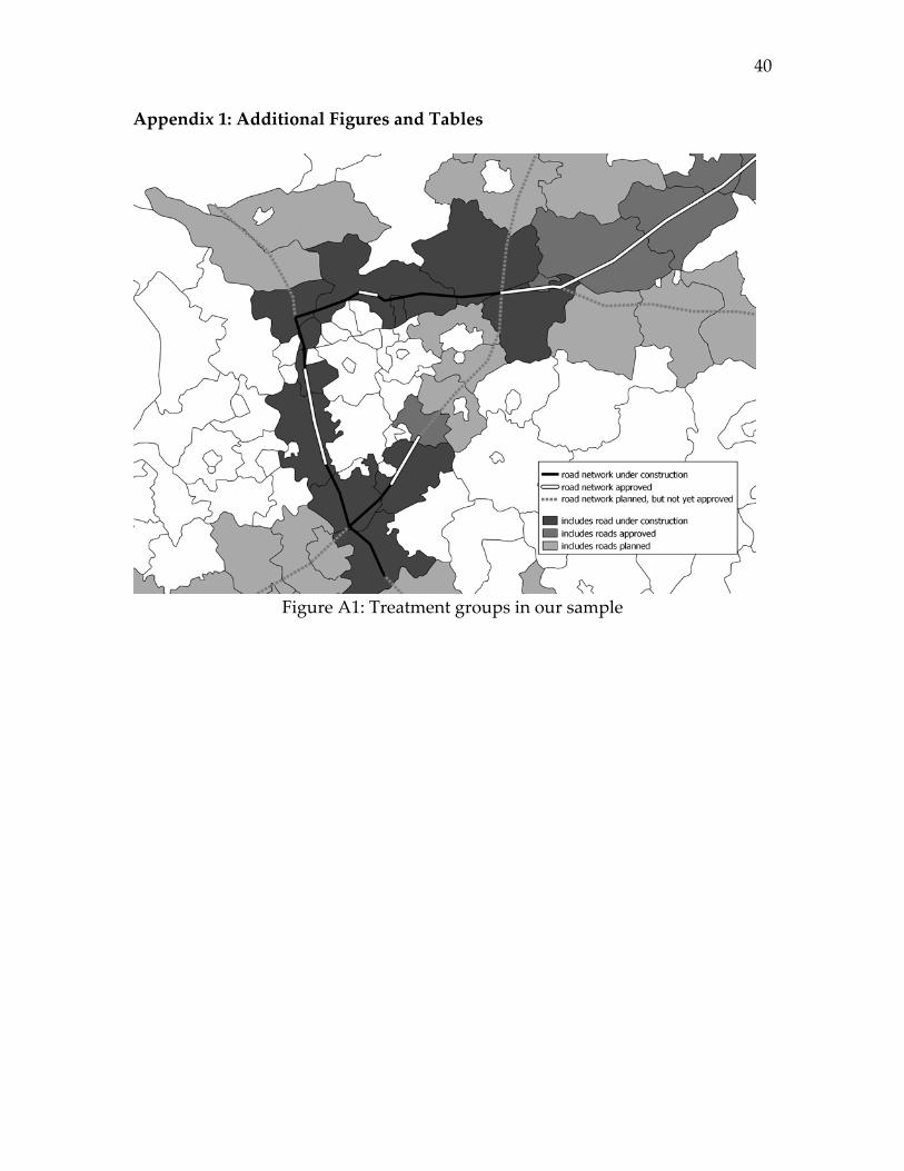
40
Appendix 1: Additional Figures and Tables
Figure A1: Treatment groups in our sample
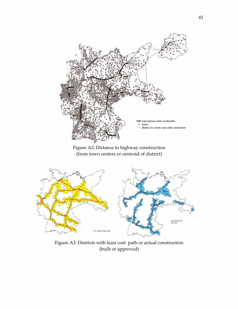
41
Figure A2: Distance to highway construction
(from town centers or centroid of district)
Figure A3: Districts with least cost path or actual construction
(built or approved)
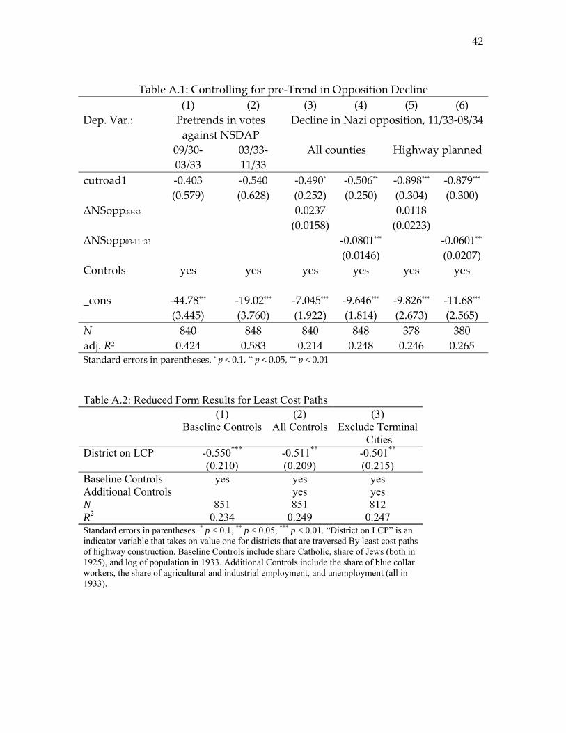
42
Table A.1: Controlling for pre‐Trend in Opposition Decline
(1) (2) (3) (4) (5) (6)
Dep. Var.: Pretrends in votes
against NSDAP
Decline in Nazi opposition, 11/33‐08/34
09/30‐
03/33
03/33‐
11/33
All counties Highway planned
cutroad1 ‐0.403 ‐0.540 ‐0.490* ‐0.506** ‐0.898*** ‐0.879***
(0.579) (0.628) (0.252) (0.250) (0.304) (0.300)
ΔNSopp30‐33 0.0237 0.0118
(0.0158) (0.0223)
ΔNSopp03‐11 ‘33 ‐0.0801*** ‐0.0601***
(0.0146) (0.0207)
Controls yes yes yes yes yes yes
_cons ‐44.78*** ‐19.02*** ‐7.045*** ‐9.646*** ‐9.826*** ‐11.68***
(3.445) (3.760) (1.922) (1.814) (2.673) (2.565)
N 840 848 840 848 378 380
adj. R2 0.424 0.583 0.214 0.248 0.246 0.265 Standard errors in parentheses. * p < 0.1, ** p < 0.05, *** p < 0.01
Table A.2: Reduced Form Results for Least Cost Paths (1) (2) (3) Baseline Controls All Controls Exclude Terminal
Cities District on LCP -0.550*** -0.511** -0.501** (0.210) (0.209) (0.215) Baseline Controls yes yes yes Additional Controls yes yes N 851 851 812 R2 0.234 0.249 0.247 Standard errors in parentheses. * p < 0.1, ** p < 0.05, *** p < 0.01. “District on LCP” is an indicator variable that takes on value one for districts that are traversed By least cost paths of highway construction. Baseline Controls include share Catholic, share of Jews (both in 1925), and log of population in 1933. Additional Controls include the share of blue collar workers, the share of agricultural and industrial employment, and unemployment (all in 1933).
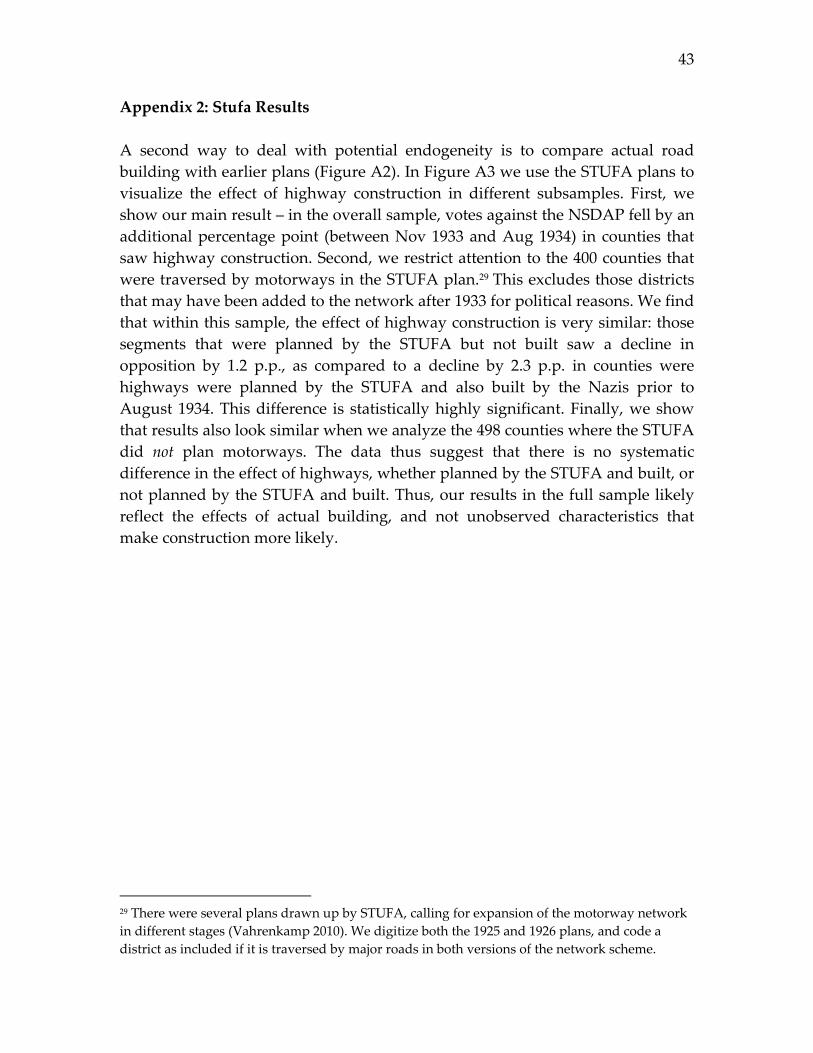
43
Appendix 2: Stufa Results
A second way to deal with potential endogeneity is to compare actual road
building with earlier plans (Figure A2). In Figure A3 we use the STUFA plans to
visualize the effect of highway construction in different subsamples. First, we
show our main result – in the overall sample, votes against the NSDAP fell by an
additional percentage point (between Nov 1933 and Aug 1934) in counties that
saw highway construction. Second, we restrict attention to the 400 counties that
were traversed by motorways in the STUFA plan.29 This excludes those districts
that may have been added to the network after 1933 for political reasons. We find
that within this sample, the effect of highway construction is very similar: those
segments that were planned by the STUFA but not built saw a decline in
opposition by 1.2 p.p., as compared to a decline by 2.3 p.p. in counties were
highways were planned by the STUFA and also built by the Nazis prior to
August 1934. This difference is statistically highly significant. Finally, we show
that results also look similar when we analyze the 498 counties where the STUFA
did not plan motorways. The data thus suggest that there is no systematic
difference in the effect of highways, whether planned by the STUFA and built, or
not planned by the STUFA and built. Thus, our results in the full sample likely
reflect the effects of actual building, and not unobserved characteristics that
make construction more likely.
29 There were several plans drawn up by STUFA, calling for expansion of the motorway network
in different stages (Vahrenkamp 2010). We digitize both the 1925 and 1926 plans, and code a
district as included if it is traversed by major roads in both versions of the network scheme.
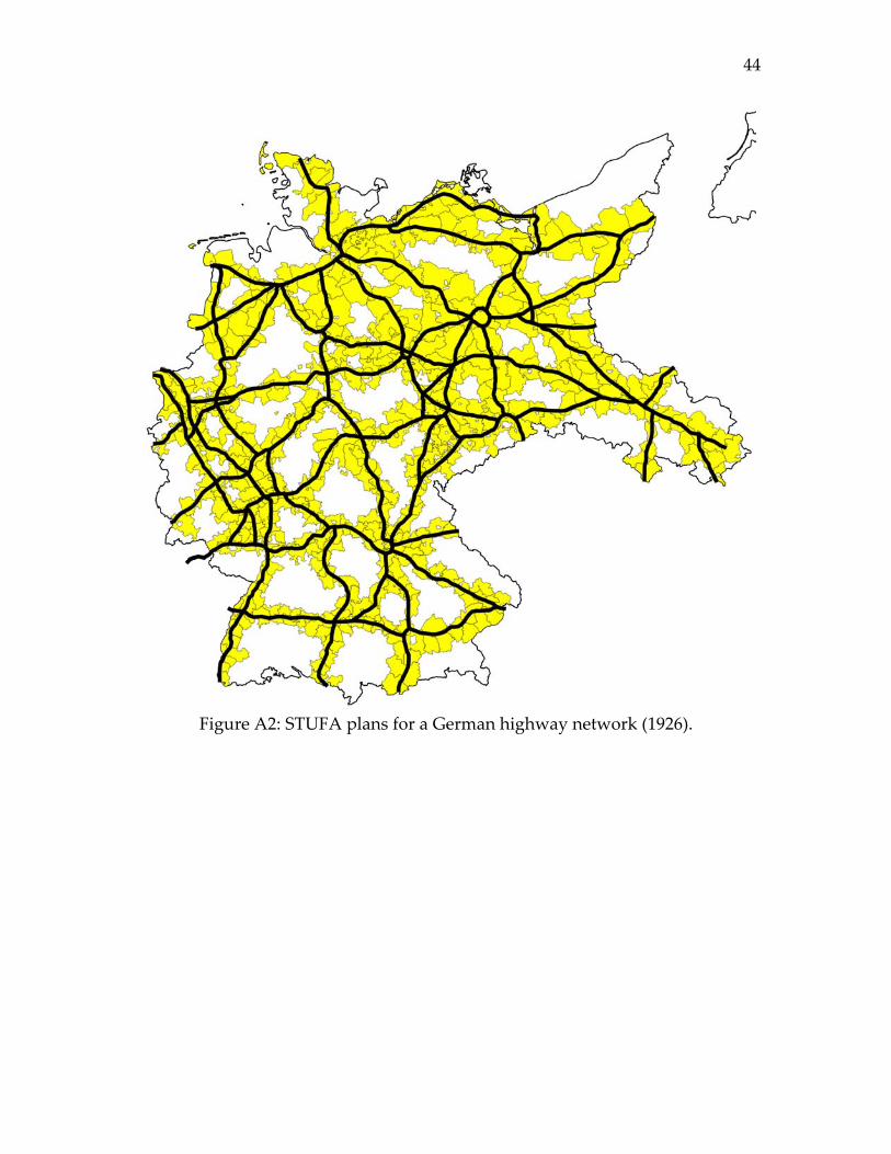
44
Figure A2: STUFA plans for a German highway network (1926).
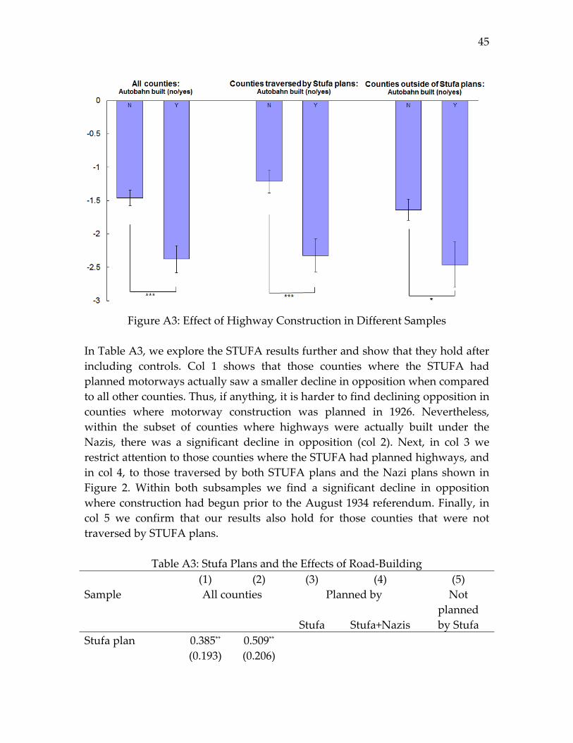
45
Figure A3: Effect of Highway Construction in Different Samples
In Table A3, we explore the STUFA results further and show that they hold after
including controls. Col 1 shows that those counties where the STUFA had
planned motorways actually saw a smaller decline in opposition when compared
to all other counties. Thus, if anything, it is harder to find declining opposition in
counties where motorway construction was planned in 1926. Nevertheless,
within the subset of counties where highways were actually built under the
Nazis, there was a significant decline in opposition (col 2). Next, in col 3 we
restrict attention to those counties where the STUFA had planned highways, and
in col 4, to those traversed by both STUFA plans and the Nazi plans shown in
Figure 2. Within both subsamples we find a significant decline in opposition
where construction had begun prior to the August 1934 referendum. Finally, in
col 5 we confirm that our results also hold for those counties that were not
traversed by STUFA plans.
Table A3: Stufa Plans and the Effects of Road‐Building
(1) (2) (3) (4) (5)
Sample All counties Planned by Not
planned
Stufa Stufa+Nazis by Stufa
Stufa plan 0.385** 0.509**
(0.193) (0.206)
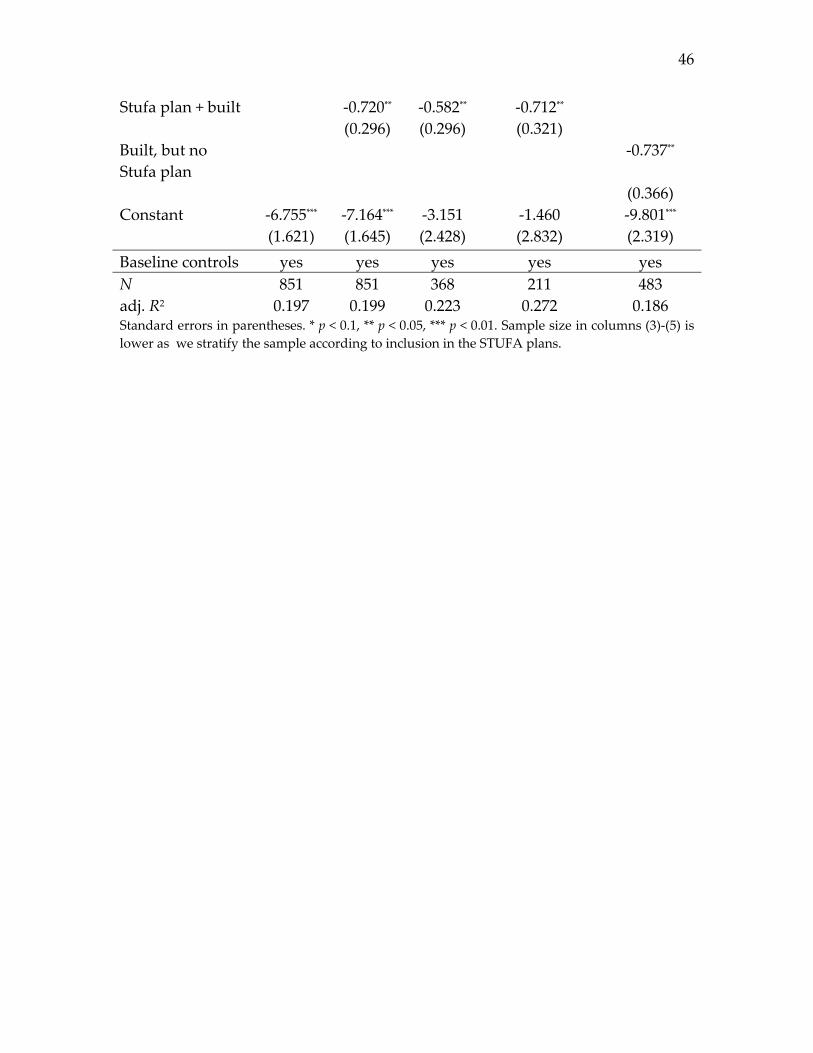
46
Stufa plan + built ‐0.720** ‐0.582** ‐0.712**
(0.296) (0.296) (0.321)
Built, but no
Stufa plan
‐0.737**
(0.366)
Constant ‐6.755*** ‐7.164*** ‐3.151 ‐1.460 ‐9.801***
(1.621) (1.645) (2.428) (2.832) (2.319)
Baseline controls yes yes yes yes yes
N 851 851 368 211 483
adj. R2 0.197 0.199 0.223 0.272 0.186 Standard errors in parentheses. * p < 0.1, ** p < 0.05, *** p < 0.01. Sample size in columns (3)‐(5) is
lower as we stratify the sample according to inclusion in the STUFA plans.