Highway Hierarchies and the Efficient Provision of Road

Services

-David Levinson

-Bhanu Yerra

Levinson, David and Bhanu Yerra (2002) Highway Costs and the Efficient Mix of State and Local Funds Transportation Research Record: Journal of the Transportation Research Board 1812 27-36. http://nexus.umn.edu/Papers/Hierarchy.pdf

Pacific Regional Science Conference, Portland 2002

Introduction

• Hierarchies in Highways and Governments

• Government layers responsible for a Highway class

• Scale Economies?

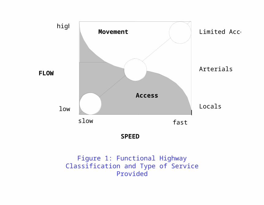
Access

Movement Limited Access

Locals

SPEED

FLOW

slow fast

high

low

Arterials

Figure 1: Functional Highway Classification and Type of Service Provided

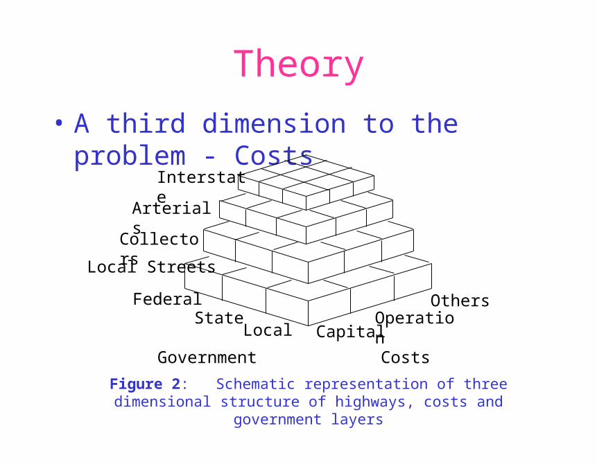
Theory

• A third dimension to the problem - Costs

CostsGovernment

Local Streets

Collectors

Arterials

Interstate

LocalState

Federal

CapitalOperation

Others

Figure 2: Schematic representation of three dimensional structure of highways, costs and government layers

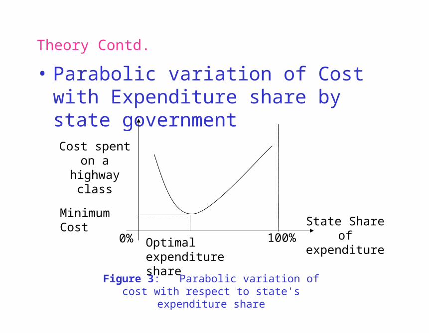
Theory Contd.

• Parabolic variation of Cost with Expenditure share by state government

State Share of expenditure

Cost spent on ahighway class

Minimum Cost

Optimal expenditure share

Figure 3: Parabolic variation of cost with respect to state's expenditure share

0% 100%

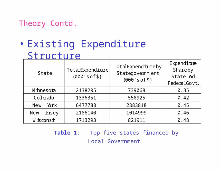
Theory Contd.

• Existing Expenditure Structure

StateTotal Expenditure

(000's of $)

Total Expenditure byState government

(000's of $)

ExpenditureShare byState And

Federal Govt.Minnesota 2138205 739068 0.35

Colorado 1336351 558925 0.42

New York 6477788 2883818 0.45

New J ersey 2186140 1014999 0.46

Wisconsin 1713293 821911 0.48

Table 1: Top five states financed by Local Government

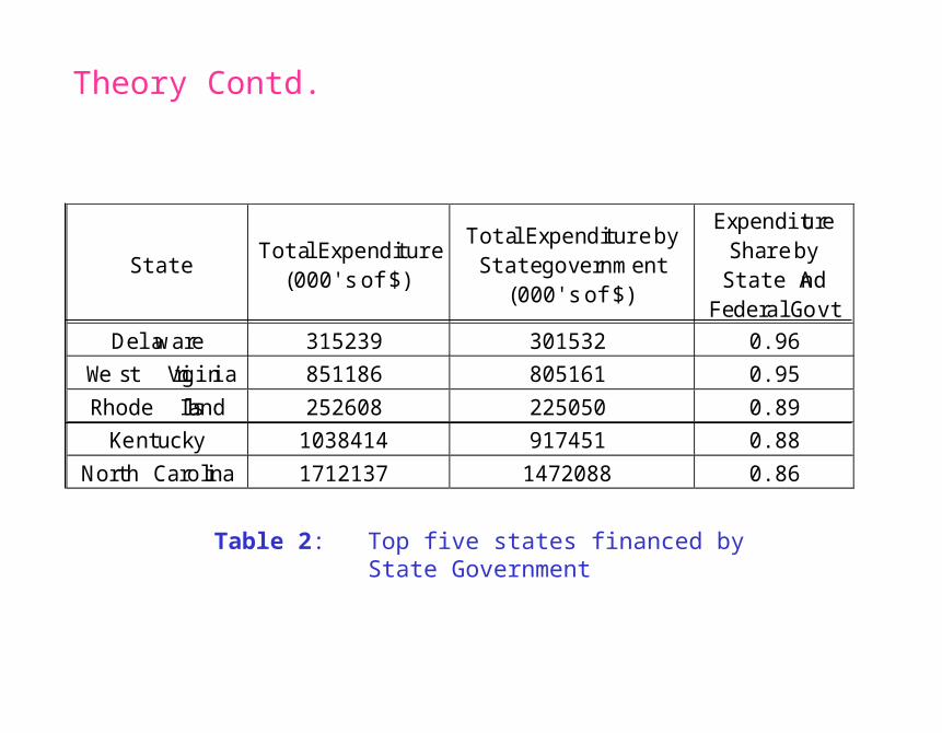
Theory Contd.

StateTotal Expenditure

(000's of $)

Total Expenditure byState government

(000's of $)

ExpenditureShare byState And

Federal GovtDelaware 315239 301532 0.96

West Virginia 851186 805161 0.95

Rhode Island 252608 225050 0.89

Kentucky 1038414 917451 0.88

North Carolina 1712137 1472088 0.86

Table 2: Top five states financed by State Government

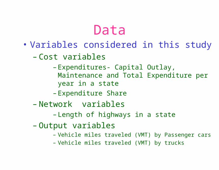
Data• Variables considered in this study

– Cost variables– Expenditures- Capital Outlay, Maintenance and

Total Expenditure per year in a state

– Expenditure Share

– Network variables– Length of highways in a state

– Output variables– Vehicle miles traveled (VMT) by Passenger cars

– Vehicle miles traveled (VMT) by trucks

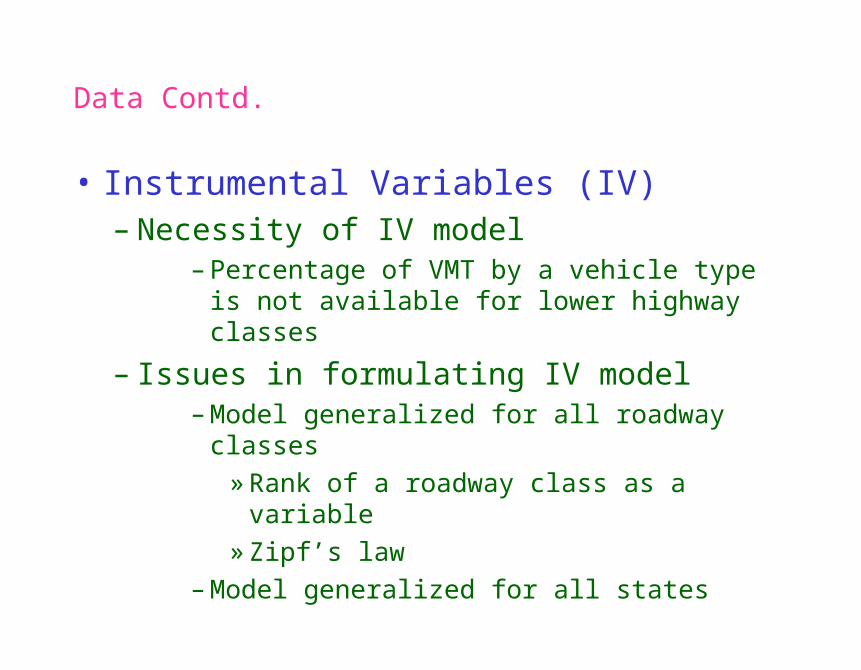
Data Contd.

• Instrumental Variables (IV)– Necessity of IV model

– Percentage of VMT by a vehicle type is not available for lower highway classes

– Issues in formulating IV model– Model generalized for all roadway classes

» Rank of a roadway class as a variable

» Zipf’s law

– Model generalized for all states

Data Contd.

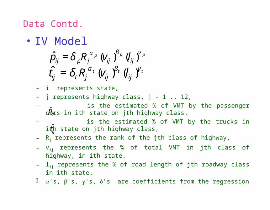
• IV Model

– i represents state,

– j represents highway class, j - 1 .. 12,

– is the estimated % of VMT by the passenger cars in ith state on jth highway class,

– is the estimated % of VMT by the trucks in ith state on jth highway class,

– Rj represents the rank of the jth class of highway,

– vij represents the % of total VMT in jth class of highway, in ith state,

– lij represents the % of road length of jth roadway class in ith state,

's, 's, 's, 's are coefficients from the regression

ˆ p ij =δpRjα p (vij )

βp (lij)γp

ˆ t ij =δtRjαt (vij )

βt (lij )γt

ˆ p ij

ˆ t ij

Data Contd.

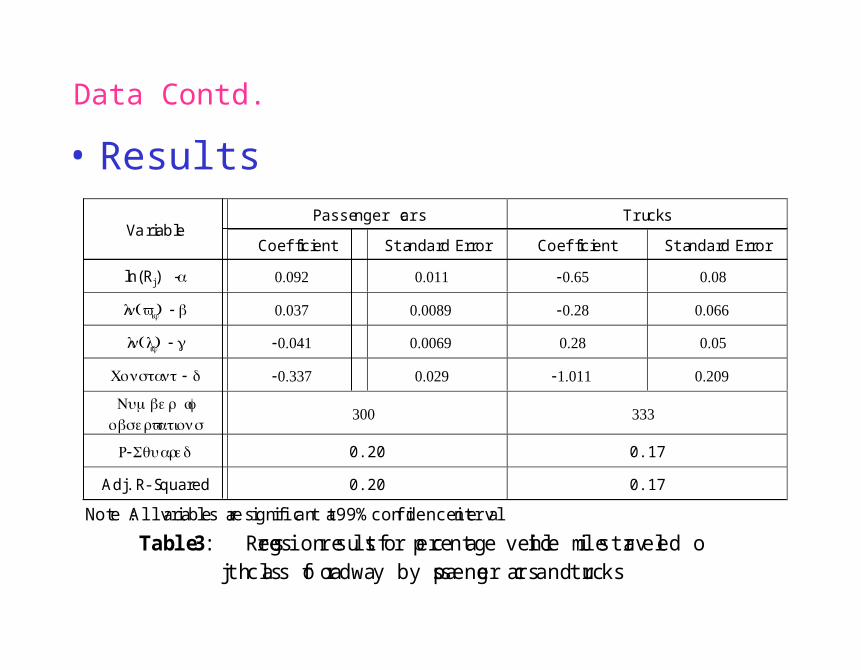
• ResultsPassenger cars Trucks

VariableCoefficient Standard Error Coefficient Standard Error

ln(Rj) - 0.092 0.011 -0.65 0.08

l (n vij) - 0.037 0.0089 -0.28 0.066

l (n lij) - -0.041 0.0069 0.28 0.05

Constan t - -0.337 0.029 -1.011 0.209

Numbe r ofobservations

300 333

-R Squared 0.20 0.17

Adj. R-Squared 0.20 0.17

Note : All variables are significant at 99% confidence interval

Table 3: Regression results for percentage vehicle miles traveled onjth class of roadway by passenger cars and trucks

Data Contd.

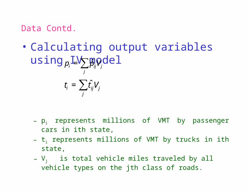
• Calculating output variables using IV model

– pi represents millions of VMT by passenger cars in ith state,

– ti represents millions of VMT by trucks in ith state,

– Vj is total vehicle miles traveled by all vehicle types on the jth class of roads.

pi = ˆ p ijVjj

∑

ti = ˆ t ijVjj

∑

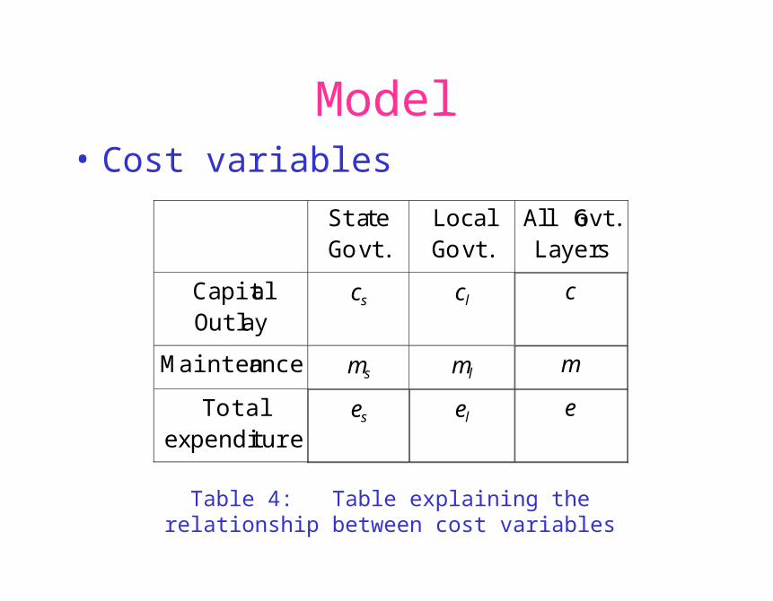
Model• Cost variables

StateGovt.

LocalGovt.

All Govt.Layers

CapitalOutlay

cs cl c

Mainten ance ms ml m

To tale xpendi t ure

es el e

Table 4: Table explaining the relationship between cost variables

Model Contd.

• Cost variables Contd.– e is total cost of capital outlay and maintenance,

– c is capital outlay cost,

– m is maintenance cost,

– es is total cost financed by state and federal government,

– el is total cost financed by local government,

– cs is capital outlay financed by state and federal government,

– cl is capital outlay financed by local government,

– ms is maintenance cost financed by state and federal government,

– ml is maintenance cost financed by the local government.

Model Contd.

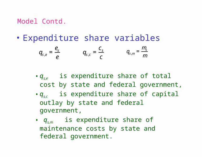
• Expenditure share variables

• qs,e is expenditure share of total cost by state and federal government,

• qs,c is expenditure share of capital outlay by state and federal government,

• qs,m is expenditure share of maintenance costs by state and federal government.

qs,e =es

eqs,c =

cs

cqs,m =

ms

m

Model Contd.

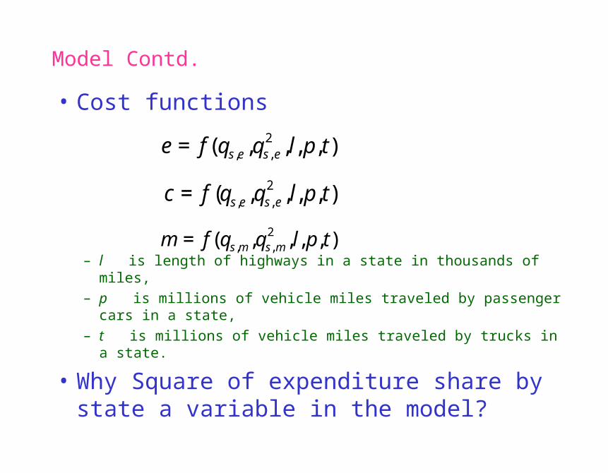
• Cost functions

– l is length of highways in a state in thousands of miles,

– p is millions of vehicle miles traveled by passenger cars in a state,

– t is millions of vehicle miles traveled by trucks in a state.

• Why Square of expenditure share by state a variable in the model?

e= f(qs,e,qs,e2 ,l,p,t)

c = f (qs,e,qs,e2 ,l,p,t)

m= f(qs,m,qs,m2 ,l,p,t)

Model Contd.

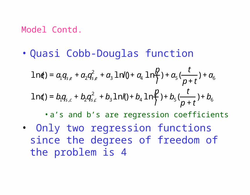
• Quasi Cobb-Douglas function

• a’s and b’s are regression coefficients

• Only two regression functions since the degrees of freedom of the problem is 4

ln(e) =a1qs,e +a2qs,e2 +a3 ln(l)+a4 ln(

pl) +a5(

tp+t

) +a6

ln(c) =b1qs,c +b2qs,c2 +b3ln(l)+b4 ln(

pl)+b5(

tp+t

)+b6

Model Contd.

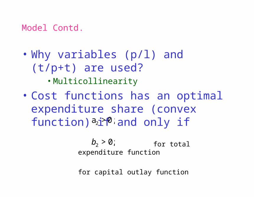
• Why variables (p/l) and (t/p+t) are used?• Multicollinearity

• Cost functions has an optimal expenditure share (convex function) if and only if

for total expenditure function

for capital outlay function

a2 >0;

b2 >0;

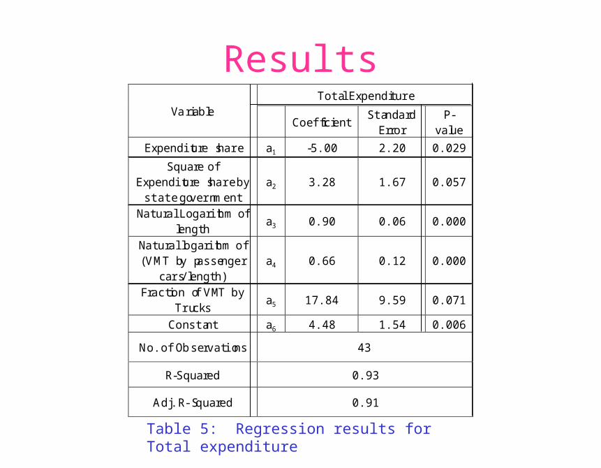
ResultsTotal Expenditure

VariableCoefficient

StandardError

P-value

Expenditure share a1 -5.00 2.20 0.029

Square ofExpenditure share by

state governmenta2 3.28 1.67 0.057

Natural Logarithm oflength

a3 0.90 0.06 0.000

Natural logarithm of(VMT by passenger

cars/ length)a4 0.66 0.12 0.000

Fraction of VMT byTrucks

a5 17.84 9.59 0.071

Constant a6 4.48 1.54 0.006

No. of Observations 43

R-Squared 0.93

Adj. R-Squared 0.91

Table 5: Regression results for Total expenditure

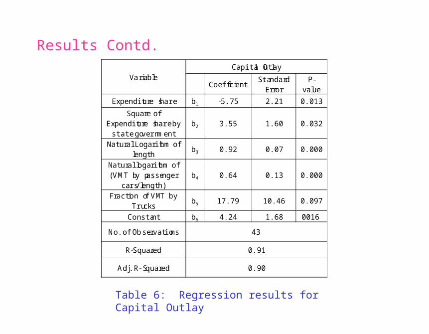
Results Contd.Capital Outlay

VariableCoefficient

StandardError

P-value

Expenditure share b1 -5.75 2.21 0.013

Square ofExpenditure share by

state governmentb2 3.55 1.60 0.032

Natural Logarithm oflength

b3 0.92 0.07 0.000

Natural logarithm of(VMT by passenger

cars/ length)b4 0.64 0.13 0.000

Fraction of VMT byTrucks

b5 17.79 10.46 0.097

Constant b6 4.24 1.68 0016

No. of Observations 43

R-Squared 0.91

Adj. R-Squared 0.90

Table 6: Regression results for Capital Outlay

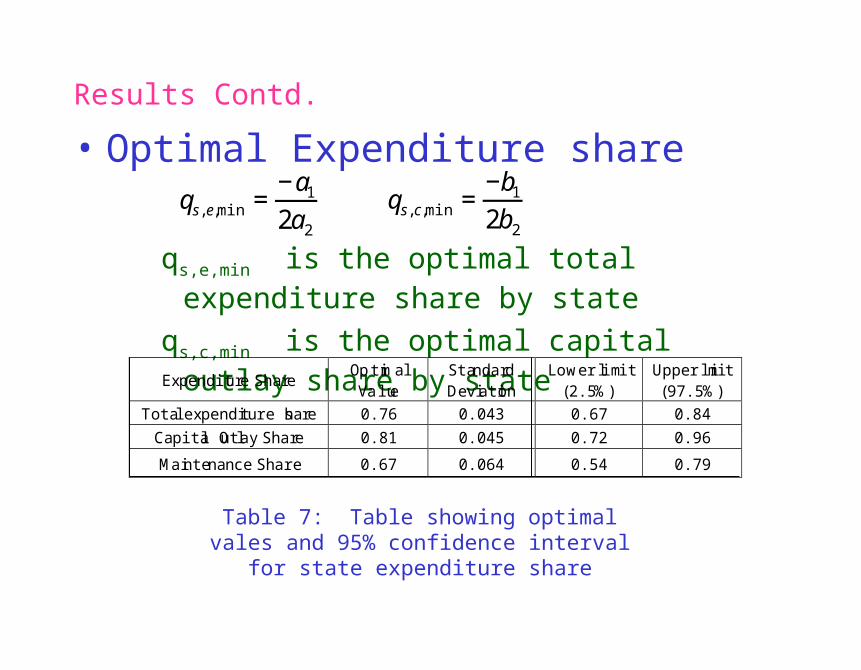
Results Contd.

• Optimal Expenditure share

qs,e,min is the optimal total expenditure share by state

qs,c,min is the optimal capital outlay share by state

qs,e,min =−a1

2a2

qs,c,min =−b1

2b2

Expenditure ShareOptimalValue

StandardDeviation

Lower limit(2.5%)

Upper limit(97.5%)

Total expenditure share 0.76 0.043 0.67 0.84

Capital Outlay Share 0.81 0.045 0.72 0.96

Maintenance Share 0.67 0.064 0.54 0.79

Table 7: Table showing optimal vales and 95% confidence interval for state expenditure share

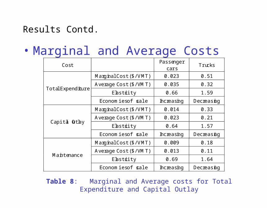
Results Contd.

• Marginal and Average CostsCost

Passengercars

Trucks

Marginal Cost ($/ VMT) 0.023 0.51

Average Cost ($/ VMT) 0.035 0.32

Elasticity 0.66 1.59Total Expenditure

Economies of scale Increasing Decreasing

Marginal Cost ($/ VMT) 0.014 0.33

Average Cost ($/ VMT) 0.023 0.21

Elasticity 0.64 1.57Capital Outlay

Economies of scale Increasing Decreasing

Marginal Cost ($/ VMT) 0.009 0.18

Average Cost ($/ VMT) 0.013 0.11

Elasticity 0.69 1.64Maintenance

Economies of scale Increasing Decreasing

Table 8: Marginal and Average costs for Total Expenditure and Capital Outlay

Conclusion and Recommendations• Parabolic nature of cost functions

• Most of the states are within the 95% confidence interval of optimal expenditure share of capital outlay

• Most of the states are out of the 95% confidence interval of optimal expenditure share of Total expenditure

• All states together can save $10 billion if all of them are at optimal point.

• Financial policies