HIGHLY IONIZED GAS IN THE GALACTIC HALO AND THE HIGH-VELOCITY

HIGHLY IONIZED GAS IN THE GALACTIC HALO AND THE HIGH-VELOCITYCLOUDS TOWARD PG 1116+2151

Rajib Ganguly,2Kenneth R. Sembach,

2Todd M. Tripp,

3and Blair D. Savage

4

Receivved 2004 October 21; accepted 2004 December 17

ABSTRACT

We have obtained high-resolution Far Ultraviolet Spectroscopic Explorer (FUSE ) and Hubble Space Telescope(HST ) Space Telescope Imaging Spectrograph (STIS) echelle observations of the quasar PG 1116þ 215 (zem ¼0:1765, l ¼ 223N36, b ¼ þ68N21). The semicontinuous coverage of the ultraviolet spectrum over the wavelengthrange 916–2800 8 provides detections of Galactic and high-velocity cloud (HVC) absorption over a wide rangeof ionization species: H i, C ii–iv, N i–ii , O i , O vi, Mg ii, Si ii–iv, P ii , S ii, and Fe ii over the velocity range�100 km s�1 < vLSR < þ200 km s�1. The high dispersion of these spectra (6.5–20 km s�1) reveals that low-ionization species consist of five discrete components: three at low and intermediate velocities (vLSR � �44, �7,+56 km s�1) and two at high velocities (vLSR � þ100, +184 km s�1). Over the same velocity range, the higherionization species (C iii–iv, O vi , Si iv)—those with ionization potentials larger than 40 eV—show continuousabsorption with column density peaks at vLSR � 10 km s�1, the expected velocity of halo gas corotating with theGalactic disk, and vLSR � þ184 km s�1, the velocity of the higher velocity HVC. The velocity coincidence of bothlow- and high-ionization species in the vLSR � þ184 km s�1 HVC gas suggests that they arise in a commonstructure, though not necessarily in the same gaseous phase. The absorption structure in the high-ionization gas,which extends to very low velocities, suggests a scenario in which a moderately dense cloud of gas is streamingaway from the Galaxy through a hot external medium (either the Galactic halo or corona) that is stripping gas fromthis cloud. The cloud core produces the observed neutral atoms and low-ionization species. The stripped material isthe likely source of the high-ionization species. Among the host of collisionally ionized nonequilibriummodels, wefind that shock ionization and conductive interfaces can account for the column density ratios of high-ionizationspecies. The nominal metallicity of the neutral gas using the O i and H i column densities is ½O=H� ��0:66, with asubstantial uncertainty caused by the saturation of the H i Lyman series in the FUSE band. The ionization of thecloud core is likely dominated by photons, and assuming the source of ionizing photons is the extragalactic UVbackground, we estimate the cloud has a density of 10�2.7 cm�3 with a thermal pressure p=k � 24 cm�3 K. Ifphotons escaping the Galactic disk are also included (i.e., if the cloud lies closer than the outer halo), the density andthermal pressure could be higher by as much as 2 dex. In either case, the relative abundances of O, Si, and Fe in thecloud core are readily explained without departures from the solar pattern. We compare the column density ratios ofthe HVCs toward the PG 1116+215 to other isolated HVCs as well as Complex C. Magellanic Stream gas (either adiffuse extension of the leading arm or gas stripped from a prior passage) is a possible origin for this gas and isconsistent with the location of the high-velocity gas on the sky, as well as its high positive velocity, the ionization ,and metallicity.

Subject headinggs: Galaxy: evolution — Galaxy: halo — ISM: abundances — ISM: clouds

Online material: color figures

1. INTRODUCTION

Recent observations with the Far Ultraviolet SpectroscopicExplorer (FUSE ) have revealed a complex network of highlyionized high-velocity gas in the vicinity of the Galaxy. This newinformation demonstrates that the high-velocity material is farmore complex than originally thought and is providing newinsight into the formation and evolution of the Milky Way. The

primary diagnostic of this gas is the O vi k1031.926 line, whichis seen in absorption at velocities exceeding�100 km s�1 in thelocal standard of rest in at least 60% of the AGN/QSO sightlines observed in the first few years of FUSE operations(Wakker et al. 2003). Sembach et al. (2003) have attributed thehigh-velocity O vi to collisionally ionized gas at the boundariesbetween warm circumgalactic clouds and a highly extended(Rk70 kpc), hot (T >106 K), low-density (nP10�4 cm�3)Galactic corona or Local Group medium. This result is sup-ported by detailed investigations of the relationship between thehighly ionized gas and lower ionization species (e.g., C ii, C iv,Si ii–iv) in high-velocity cloud Complex C (Fox et al. 2004)and the high-velocity clouds (HVCs) along the sight line towardPKS 2155�304 (Sembach et al. 1999; Collins et al. 2005). Analternate explanation for the origin of the high-velocity O vi—photoionization in a low-density plasma—has also been con-sidered (Nicastro et al. 2002) but is difficult to reconcile with dataavailable for the other O viHVCs (Sembach et al. 2004b; Collinset al. 2005).

1 Based on observations made with the NASA/ESA Hubble Space Tele-scope, which is operated by the Association of Universities for Research inAstronomy, Inc., under NASA contract NAS 5-26555. Also based on observa-tions made with the NASA-CNES-CSA Far Ultraviolet Spectroscopic Ex-plorer, which is operated for NASA by Johns Hopkins University under NASAcontract NAS 5-32985.

2 Space Telescope Science Institute, 3700 San Martin Drive, Baltimore,MD 21218.

3 Department of Astronomy, University of Massachusetts, Amherst,MA 01003.

4 Department of Astronomy, University of Wisconsin—Madison, 475North Charter Street, Madison, WI 53706.

A

251

The Astrophysical Journal Supplement Series, 157:251–278, 2005 April

# 2005. The American Astronomical Society. All rights reserved. Printed in U.S.A.

Establishing the relationship of the high-velocity O vi withlower ionization gas and pinpointing its possible origins re-quires high-resolution observations of other ionization stageswith the Hubble Space Telescope (HST ). We have obtainedSpace Telescope Imaging Spectrograph (STIS) observations ofthe bright quasar PG 1116+215 (l ¼ 223N36, b ¼ þ68N21,mV �15:2, zem ¼ 0:1765) to study the high-velocity O vi in a direc-tion that is well away from large concentrations of high-velocityH i observable in 21 cm emission (e.g., the Magellanic Stream,Complexes A, C, M). High-velocity gas in this sight line wasfirst noted by Tripp et al. (1998), using HST observations withthe Goddard High Resolution Spectrograph. The sight line con-tains high-velocity O vi at vLSR � þ184 km s�1 (Sembach et al.2003). High-velocity gas in this general region of the sky isoften purported to be extragalactic in nature based upon itskinematical properties (Blitz et al. 1999;Nicastro et al. 2003—butsee B. P. Wakker 2005, in preparation, for a rebuttal to thesearguments). PG 1116+215 is on the opposite side of the sky fromthe PKS 2155�304 and Mrk 509 sight lines, which are the onlyother isolated HVCs to have had their ionization properties stud-ied in detail. It therefore presents an excellent case to test whetherthe ionization and kinematical properties of the O vi and otherionization stages are consistent with an extragalactic location.The sight line passes through the hot gas of the Galactic halo aswell as several intermediate-velocity clouds located within a fewkiloparsecs of the Galactic disk (e.g., Wakker 2004 and refer-ences therein). Thus, observations of this single sight line alsoprovide self-contained absorption fiducials against which to judgethe character of the high-velocity absorption.

A complete spectral catalog of the FUSE and HST SpaceTelescope Imaging Spectrograph (STIS) observations for thePG 1116+215 sight line is presented in a companion studyby Sembach et al. (2004a). Information about the intergalacticabsorption-line systems along the PG 1116+215 sight line canbe found in that paper. In x 2, we present the spectroscopic dataavailable for the Galactic and high-velocity absorption in thesight line. In x 3, we provide a general overview of the absorp-tion profiles and make preliminary assessments of the kinemat-ics of the Galactic absorption and the high-velocity gas. In x 4,we describe our methodology for line measurements (e.g., equiv-alent widths, column densities) and present these for selectedregions of the absorption profiles. In addition, we present com-posite apparent column density profiles for a sample of impor-tant species. In the following sections, we discuss and analyzethe Galactic and intermediate-velocity absorption (x 5), thehigh-velocity absorption at vLSR � 100 km s�1 (x 6), and thehigh-velocity absorption at vLSR � 184 km s�1 (x 7). Finally,we discuss the implications of this study and summarize ourfindings in xx 8 and 9, respectively.

2. OBSERVATIONS AND DATA PROCESSING

We observed PG 1116+215 with FUSE on two separate oc-casions in 2000 April and 2001 April. For all observations PG1116+215 was aligned in the center of the LiF1 channel LWRS(3000 ; 3000) aperture used for guiding. The remaining channels(SiC1, SiC2, and LiF2) were coaligned throughout the obser-vations. The total exposure time was 77 ks in the LiF channelsand 64 ks in the SiC channels after screening the time-taggedphoton event lists for valid data. We processed the FUSE datawith a customized version of the standard FUSE pipeline soft-ware (CALFUSE ver. 2.2.2). The data have continuum signal-to-noise ratios S=N�18 and 14 per 0.07 8 (20–22 km s�1)spectral resolution element in the LiF1 and LiF2 channels at

1050 8, and S=N� 8 and 13 at 950 8 in the SiC1 and SiC2channels. The zero-point velocity uncertainty and cross-channelrelative velocity uncertainties are roughly 5 km s�1. Further in-formation about the acquisition and processing of the FUSE datacan be found in Sembach et al. (2004a). A description of FUSEand its on-orbit performance can be found in articles by Mooset al. (2000) and Sahnow et al. (2000).We observed PG 1116+215 with HST STIS in 2000 May–

June with the E140M grating and 0B2 ; 0B06 slit for an exposuretime of 20 ks. We also obtained 5.6 ks of E230M data throughthe 0B2 ; 0B09 slit. We followed the standard data reduction andcalibration procedures used in our previous STIS investigations(see Tripp et al. 2001; Sembach et al. 2004a). The STIS data havea spectral resolution of 6.5 km s�1 (FWHM) for the E140Mgrating, and 10 km s�1 (FWHM) for the E230M grating , bothwith a sampling of 2–3 pixels per resolution element. The zero-point heliocentric velocity uncertainty is about 0.5 pixels, or�1.5 km s�1 for E140M, and �2.5 km s�1 for E230M (Proffittet al. 2002). The E140M spectra have S=N � 14 15 per reso-lution element at 1300 and 1500 8. The E230M spectra haveS=N � 6:6 8 per resolution element at 2400 and 2800 8. Foradditional information about STIS, see Woodgate et al. (1998),Kimble et al. (1998), and Proffitt et al. (2002). We plot sampleFUSE and STIS spectra in Figure 1. The three panels are scaledto cover the same total velocity extent. Interstellar absorptionfeatures are labeled , and high-velocity lines are indicated withoffset tic marks.

Fig. 1.—Portions of the spectra from the three observations used in thispaper: FUSE (top), HST STIS-E140M (middle), and HST STIS-E230M (bot-tom). The plotted regions are centered around key transitions from each obser-vation, and the wavelength scale shown spans about 3300 km s�1 in all threepanels. In each panel, the Galactic ISM profiles are labeled with the absorbingspecies, and the corresponding +184 km s�1 HVC absorption are indicated bythe offset tic marks.

GANGULY ET AL.252 Vol. 157

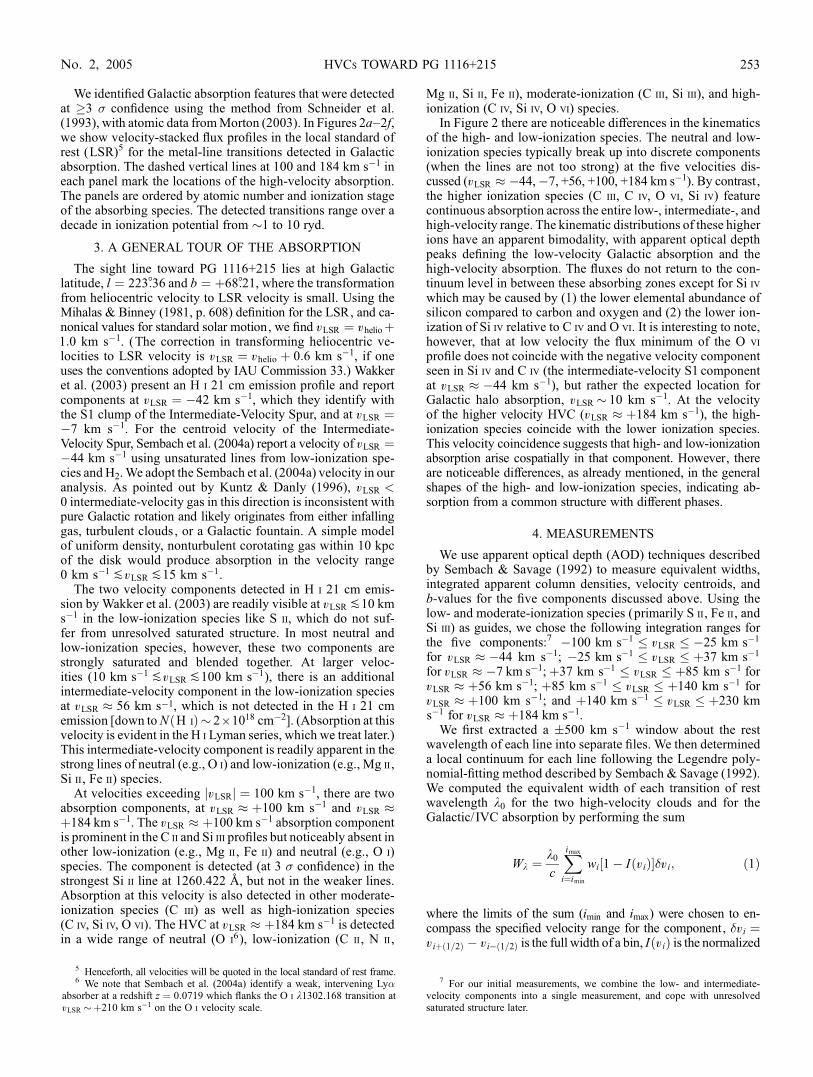
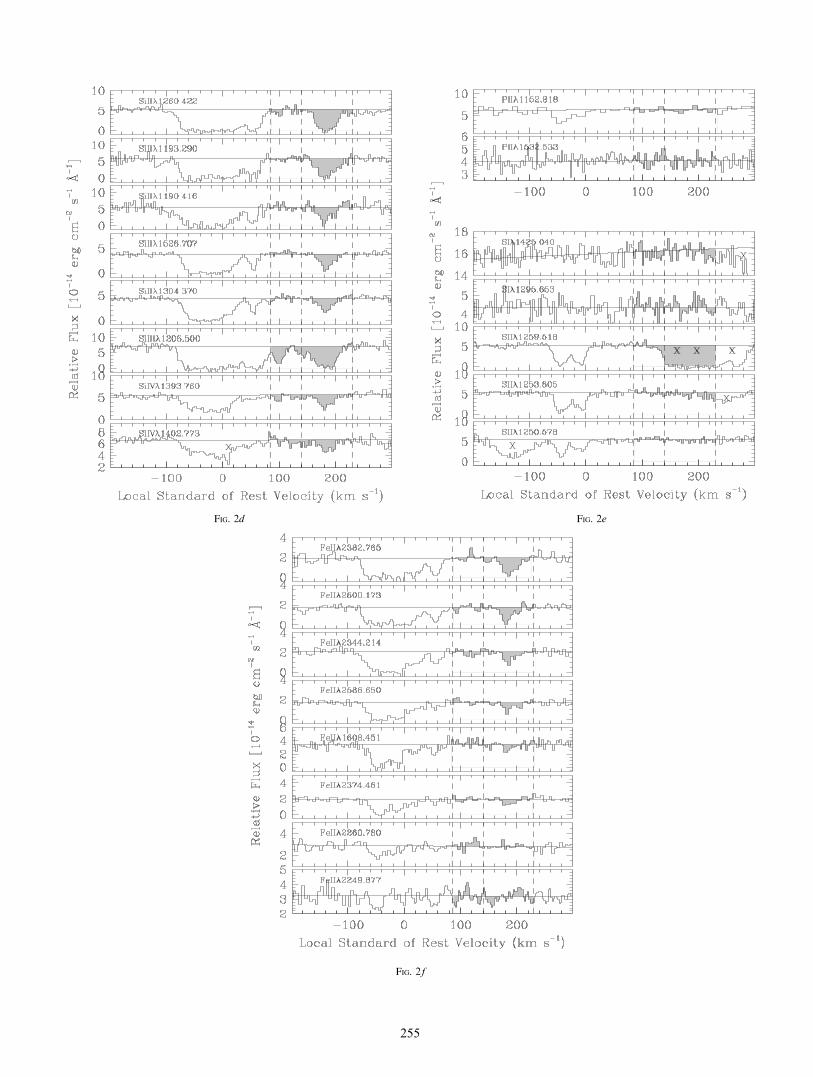
We identified Galactic absorption features that were detectedat �3 � confidence using the method from Schneider et al.(1993), with atomic data fromMorton (2003). In Figures 2a–2f,we show velocity-stacked flux profiles in the local standard ofrest (LSR)5 for the metal-line transitions detected in Galacticabsorption. The dashed vertical lines at 100 and 184 km s�1 ineach panel mark the locations of the high-velocity absorption.The panels are ordered by atomic number and ionization stageof the absorbing species. The detected transitions range over adecade in ionization potential from �1 to 10 ryd.

3. A GENERAL TOUR OF THE ABSORPTION

The sight line toward PG 1116+215 lies at high Galacticlatitude, l ¼ 223N36 and b ¼ þ68N21, where the transformationfrom heliocentric velocity to LSR velocity is small. Using theMihalas & Binney (1981, p. 608) definition for the LSR, and ca-nonical values for standard solar motion, we find vLSR ¼ v helioþ1:0 km s�1. (The correction in transforming heliocentric ve-locities to LSR velocity is vLSR ¼ v helio þ 0:6 km s�1, if oneuses the conventions adopted by IAU Commission 33.) Wakkeret al. (2003) present an H i 21 cm emission profile and reportcomponents at vLSR ¼ �42 km s�1, which they identify withthe S1 clump of the Intermediate-Velocity Spur, and at vLSR ¼�7 km s�1. For the centroid velocity of the Intermediate-Velocity Spur, Sembach et al. (2004a) report a velocity of vLSR ¼�44 km s�1 using unsaturated lines from low-ionization spe-cies and H2.We adopt the Sembach et al. (2004a) velocity in ouranalysis. As pointed out by Kuntz & Danly (1996), vLSR <0 intermediate-velocity gas in this direction is inconsistent withpure Galactic rotation and likely originates from either infallinggas, turbulent clouds , or a Galactic fountain. A simple modelof uniform density, nonturbulent corotating gas within 10 kpcof the disk would produce absorption in the velocity range0 km s�1 PvLSR P15 km s�1.

The two velocity components detected in H i 21 cm emis-sion by Wakker et al. (2003) are readily visible at vLSR P10 kms�1 in the low-ionization species like S ii, which do not suf-fer from unresolved saturated structure. In most neutral andlow-ionization species, however, these two components arestrongly saturated and blended together. At larger veloc-ities (10 km s�1 PvLSR P100 km s�1), there is an additionalintermediate-velocity component in the low-ionization speciesat vLSR � 56 km s�1, which is not detected in the H i 21 cmemission [down toNðH iÞ � 2 ; 1018 cm�2]. (Absorption at thisvelocity is evident in the H i Lyman series, which we treat later.)This intermediate-velocity component is readily apparent in thestrong lines of neutral (e.g., O i) and low-ionization (e.g., Mg ii ,Si ii, Fe ii) species.

At velocities exceeding jvLSRj ¼ 100 km s�1, there are twoabsorption components, at vLSR � þ100 km s�1 and vLSR �þ184 km s�1. The vLSR � þ100 km s�1 absorption componentis prominent in the C ii and Si iii profiles but noticeably absent inother low-ionization (e.g., Mg ii, Fe ii) and neutral (e.g., O i)species. The component is detected (at 3 � confidence) in thestrongest Si ii line at 1260.422 8, but not in the weaker lines.Absorption at this velocity is also detected in other moderate-ionization species (C iii) as well as high-ionization species(C iv, Si iv, O vi). The HVC at vLSR � þ184 km s�1 is detectedin a wide range of neutral (O i

6), low-ionization (C ii, N ii ,

Mg ii, Si ii, Fe ii), moderate-ionization (C iii, Si iii), and high-ionization (C iv, Si iv, O vi) species.

In Figure 2 there are noticeable differences in the kinematicsof the high- and low-ionization species. The neutral and low-ionization species typically break up into discrete components(when the lines are not too strong) at the five velocities dis-cussed (vLSR � �44,�7, +56, +100, +184 km s�1). By contrast,the higher ionization species (C iii, C iv, O vi, Si iv) featurecontinuous absorption across the entire low-, intermediate-, andhigh-velocity range. The kinematic distributions of these higherions have an apparent bimodality, with apparent optical depthpeaks defining the low-velocity Galactic absorption and thehigh-velocity absorption. The fluxes do not return to the con-tinuum level in between these absorbing zones except for Si ivwhich may be caused by (1) the lower elemental abundance ofsilicon compared to carbon and oxygen and (2) the lower ion-ization of Si iv relative to C iv and O vi. It is interesting to note,however, that at low velocity the flux minimum of the O vi

profile does not coincide with the negative velocity componentseen in Si iv and C iv (the intermediate-velocity S1 componentat vLSR � �44 km s�1), but rather the expected location forGalactic halo absorption, vLSR � 10 km s�1. At the velocityof the higher velocity HVC (vLSR � þ184 km s�1), the high-ionization species coincide with the lower ionization species.This velocity coincidence suggests that high- and low-ionizationabsorption arise cospatially in that component. However, thereare noticeable differences, as already mentioned, in the generalshapes of the high- and low-ionization species, indicating ab-sorption from a common structure with different phases.

4. MEASUREMENTS

We use apparent optical depth (AOD) techniques describedby Sembach & Savage (1992) to measure equivalent widths,integrated apparent column densities, velocity centroids, andb-values for the five components discussed above. Using thelow- and moderate-ionization species (primarily S ii, Fe ii, andSi iii) as guides, we chose the following integration ranges forthe five components:7 �100 km s�1 � vLSR � �25 km s�1

for vLSR � �44 km s�1; �25 km s�1 � vLSR � þ37 km s�1

for vLSR � �7 km s�1;þ37 km s�1 � vLSR � þ85 km s�1 forvLSR � þ56 km s�1; þ85 km s�1 � vLSR � þ140 km s�1 forvLSR � þ100 km s�1; and þ140 km s�1 � vLSR � þ230 kms�1 for vLSR � þ184 km s�1.We first extracted a �500 km s�1 window about the rest

wavelength of each line into separate files. We then determineda local continuum for each line following the Legendre poly-nomial-fitting method described by Sembach & Savage (1992).We computed the equivalent width of each transition of restwavelength k0 for the two high-velocity clouds and for theGalactic/ IVC absorption by performing the sum

Wk ¼k0c

Ximax

i¼imin

wi½1� Iðv iÞ��v i; ð1Þ

where the limits of the sum (imin and imax) were chosen to en-compass the specified velocity range for the component, �v i ¼v iþð1=2Þ � v i�ð1=2Þ is the full width of a bin, Iðv iÞ is the normalized

7 For our initial measurements, we combine the low- and intermediate-velocity components into a single measurement, and cope with unresolvedsaturated structure later.

5 Henceforth, all velocities will be quoted in the local standard of rest frame.6 We note that Sembach et al. (2004a) identify a weak, intervening Ly�

absorber at a redshift z ¼ 0:0719 which flanks the O i k1302.168 transition atvLSR �þ210 km s�1 on the O i velocity scale.

HVCs TOWARD PG 1116+215 253No. 2, 2005

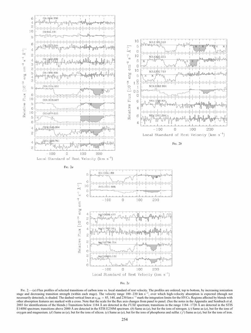
Fig. 2aFig. 2bFig. 2cFig. 2dFig. 2eFig. 2fFig. 2.—(a) Flux profiles of selected transitions of carbon ions vs. local standard of rest velocity. The profiles are ordered, top to bottom, by increasing ionization

stage and decreasing transition strength (within each stage). The velocity range 100–230 km s�1, over which high-velocity absorption is expected (though notnecessarily detected), is shaded. The dashed vertical lines at vLSR ¼ 85, 140, and 230 km s�1 mark the integration limits for the HVCs. Regions affected by blends withother absorption features are marked with a cross. Note that the scale for the flux axis changes from panel to panel. (See the notes in the Appendix and Sembach et al.2003 for identifications of the blends.) Transitions below 1184 8 are detected in the FUSE spectrum; transitions in the range 1184–1720 8 are detected in the STISE140M spectrum; transitions above 2000 8 are detected in the STIS E230M spectrum. (b) Same as (a), but for the ions of nitrogen. (c) Same as (a), but for the ions ofoxygen and magnesium. (d ) Same as (a), but for the ions of silicon. (e) Same as (a), but for the ions of phosphorus and sulfur. ( f ) Same as (a), but for the ions of iron.

Fig. 2b

Fig. 2a

Fig. 2c

254

255

Fig. 2 f

Fig. 2d Fig. 2e

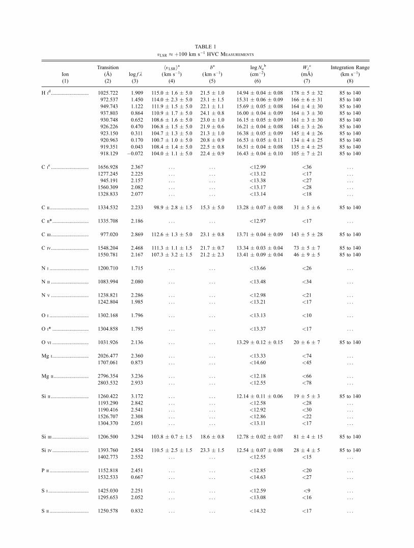
TABLE 1

vLSR � þ100 km s�1HVC Measurements

Ion

(1)

Transition

(8)(2)

log f k(3)

hvLSRia( km s�1)

(4)

ba

( km s�1)

(5)

logNab

(cm�2)

(6)

Wkc

(m8)(7)

Integration Range

(km s�1)

(8)

H id ............................ 1025.722 1.909 115.0 � 1.6 � 5.0 21.5 � 1.0 14.94 � 0.04 � 0.08 178 � 5 � 32 85 to 140

972.537 1.450 114.0 � 2.3 � 5.0 23.1 � 1.5 15.31 � 0.06 � 0.09 166 � 6 � 31 85 to 140

949.743 1.122 111.9 � 1.5 � 5.0 22.1 � 1.1 15.69 � 0.05 � 0.08 164 � 4 � 30 85 to 140

937.803 0.864 110.9 � 1.7 � 5.0 24.1 � 0.8 16.00 � 0.04 � 0.09 164 � 3 � 30 85 to 140

930.748 0.652 108.6 � 1.6 � 5.0 23.0 � 1.0 16.15 � 0.05 � 0.09 161 � 3 � 30 85 to 140

926.226 0.470 106.8 � 1.5 � 5.0 21.9 � 0.6 16.21 � 0.04 � 0.08 148 � 3 � 26 85 to 140

923.150 0.311 104.7 � 1.3 � 5.0 21.3 � 1.0 16.38 � 0.05 � 0.09 145 � 4 � 26 85 to 140

920.963 0.170 100.7 � 1.0 � 5.0 20.8 � 0.9 16.53 � 0.05 � 0.11 134 � 4 � 25 85 to 140

919.351 0.043 108.4 � 1.4 � 5.0 22.5 � 0.8 16.51 � 0.04 � 0.08 135 � 4 � 25 85 to 140

918.129 �0.072 104.0 � 1.1 � 5.0 22.4 � 0.9 16.43 � 0.04 � 0.10 105 � 7 � 21 85 to 140

C ie ............................ 1656.928 2.367 . . . . . . <12.99 <36 . . .

1277.245 2.225 . . . . . . <13.12 <17 . . .945.191 2.157 . . . . . . <13.38 <27 . . .

1560.309 2.082 . . . . . . <13.17 <28 . . .

1328.833 2.077 . . . . . . <13.14 <18 . . .

C ii............................. 1334.532 2.233 98.9 � 2.8 � 1.5 15.3 � 5.0 13.28 � 0.07 � 0.08 31 � 5 � 6 85 to 140

C ii*........................... 1335.708 2.186 . . . . . . <12.97 <17 . . .

C iii............................ 977.020 2.869 112.6 � 1.3 � 5.0 23.1 � 0.8 13.71 � 0.04 � 0.09 143 � 5 � 28 85 to 140

C iv............................ 1548.204 2.468 111.3 � 1.1 � 1.5 21.7 � 0.7 13.34 � 0.03 � 0.04 73 � 5 � 7 85 to 140

1550.781 2.167 107.3 � 3.2 � 1.5 21.2 � 2.3 13.41 � 0.09 � 0.04 46 � 9 � 5 85 to 140

N i ............................. 1200.710 1.715 . . . . . . <13.66 <26 . . .

N ii ............................ 1083.994 2.080 . . . . . . <13.48 <34 . . .

N v ............................ 1238.821 2.286 . . . . . . <12.98 <21 . . .1242.804 1.985 . . . . . . <13.21 <17 . . .

O i ............................. 1302.168 1.796 . . . . . . <13.13 <10 . . .

O i* ........................... 1304.858 1.795 . . . . . . <13.37 <17 . . .

O vi ........................... 1031.926 2.136 . . . . . . 13.29 � 0.12 � 0.15 20 � 6 � 7 85 to 140

Mg i........................... 2026.477 2.360 . . . . . . <13.33 <74 . . .

1707.061 0.873 . . . . . . <14.60 <45 . . .

Mg ii.......................... 2796.354 3.236 . . . . . . <12.18 <66 . . .

2803.532 2.933 . . . . . . <12.55 <78 . . .

Si ii ............................ 1260.422 3.172 . . . . . . 12.14 � 0.11 � 0.06 19 � 5 � 3 85 to 140

1193.290 2.842 . . . . . . <12.58 <28 . . .

1190.416 2.541 . . . . . . <12.92 <30 . . .

1526.707 2.308 . . . . . . <12.86 <22 . . .

1304.370 2.051 . . . . . . <13.11 <17 . . .

Si iii ........................... 1206.500 3.294 103.8 � 0.7 � 1.5 18.6 � 0.8 12.78 � 0.02 � 0.07 81 � 4 � 15 85 to 140

Si iv ........................... 1393.760 2.854 110.5 � 2.5 � 1.5 23.3 � 1.5 12.54 � 0.07 � 0.08 28 � 4 � 5 85 to 140

1402.773 2.552 . . . . . . <12.55 <15 . . .

P ii ............................. 1152.818 2.451 . . . . . . <12.85 <20 . . .1532.533 0.667 . . . . . . <14.63 <27 . . .

S i .............................. 1425.030 2.251 . . . . . . <12.59 <9 . . .

1295.653 2.052 . . . . . . <13.08 <16 . . .

S ii ............................. 1250.578 0.832 . . . . . . <14.32 <17 . . .

flux profile as a function of velocity, and wi is a weight that ac-counts for the fractional bins at the edges of the summation.

The integrated apparent column density, AOD-weighted cen-troid velocity, and b-value are all derived as moments of theapparent optical depth distribution. To compute these quanti-ties , we first transform the normalized flux profiles to apparentcolumn density (ACD) profiles via

Naðv iÞ ¼mec

�e21

f k0ln

1

Iðv iÞ

� �; ð2Þ

where f is the oscillator strength of the transition. From theACD profiles, the desired quantities are computed via

N ð jÞa ¼

Ximax

i¼imin

wivjNaðv iÞ�v i

Na ¼ N ð0Þa

hvi ¼ N ð1Þa =N ð0Þ

a

b2 ¼ 2 ;N ð2Þa =N ð0Þ

a : ð3Þ

In the integrations involving moments of the apparent columndensity for strongly saturated lines, we treat pixels with negativeflux (due to statistics) as having the flux equal to the rms un-certainty derived from the fit to the continuum regions adjoiningthe line. We note that this causes the derived NaðvÞ to be smallerthan the true NaðvÞ (see eq. [2]) and the derived values of Na, hvi,and b will also be affected (see eq. [3]). All other pixels aretreated in the normal way, including those with fluxes above thecontinuum level where the implied apparent column density isnegative. Since the moments of the optical depth for weak/nar-row features are very sensitive to the choice of integration range,we only report mean velocities and b-values for lines whoseequivalent width exceeds 5 times its 1 � error.

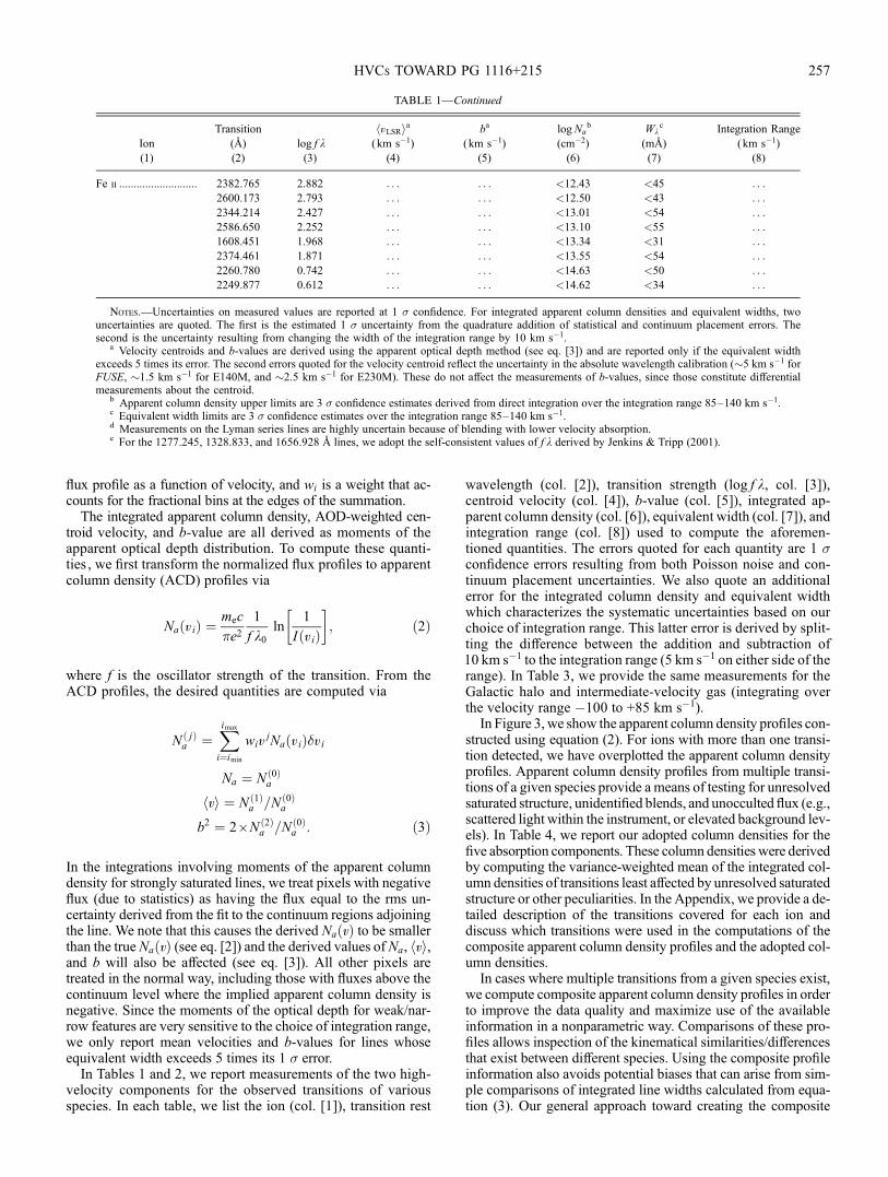
In Tables 1 and 2, we report measurements of the two high-velocity components for the observed transitions of variousspecies. In each table, we list the ion (col. [1]), transition rest

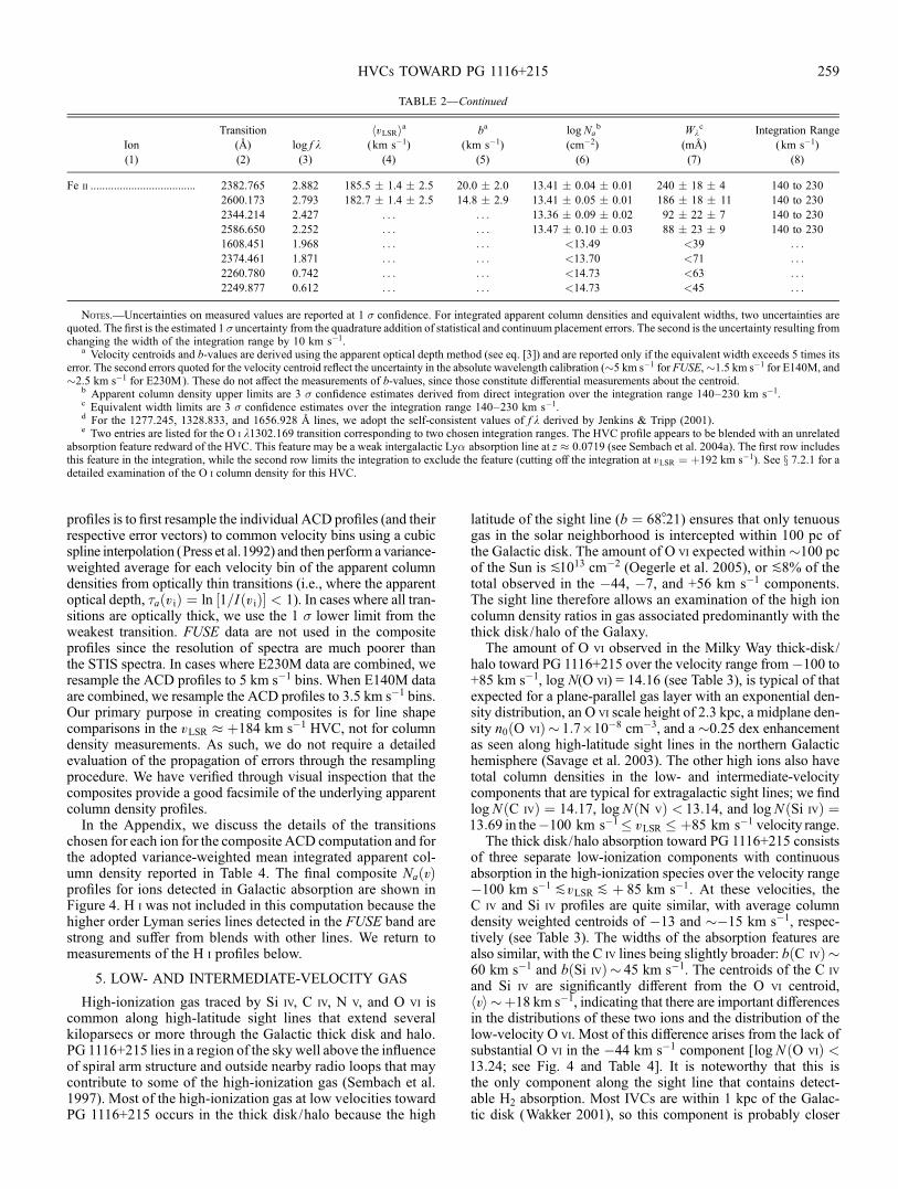
wavelength (col. [2]), transition strength (log f k, col. [3]),centroid velocity (col. [4]), b-value (col. [5]), integrated ap-parent column density (col. [6]), equivalent width (col. [7]), andintegration range (col. [8]) used to compute the aforemen-tioned quantities. The errors quoted for each quantity are 1 �confidence errors resulting from both Poisson noise and con-tinuum placement uncertainties. We also quote an additionalerror for the integrated column density and equivalent widthwhich characterizes the systematic uncertainties based on ourchoice of integration range. This latter error is derived by split-ting the difference between the addition and subtraction of10 km s�1 to the integration range (5 km s�1 on either side of therange). In Table 3, we provide the same measurements for theGalactic halo and intermediate-velocity gas (integrating overthe velocity range �100 to +85 km s�1).

In Figure 3, we show the apparent column density profiles con-structed using equation (2). For ions with more than one transi-tion detected, we have overplotted the apparent column densityprofiles. Apparent column density profiles from multiple transi-tions of a given species provide a means of testing for unresolvedsaturated structure, unidentified blends, and unocculted flux (e.g.,scattered light within the instrument, or elevated background lev-els). In Table 4, we report our adopted column densities for thefive absorption components. These column densities were derivedby computing the variance-weighted mean of the integrated col-umn densities of transitions least affected by unresolved saturatedstructure or other peculiarities. In the Appendix, we provide a de-tailed description of the transitions covered for each ion anddiscuss which transitions were used in the computations of thecomposite apparent column density profiles and the adopted col-umn densities.

In cases where multiple transitions from a given species exist,we compute composite apparent column density profiles in orderto improve the data quality and maximize use of the availableinformation in a nonparametric way. Comparisons of these pro-files allows inspection of the kinematical similarities/differencesthat exist between different species. Using the composite profileinformation also avoids potential biases that can arise from sim-ple comparisons of integrated line widths calculated from equa-tion (3). Our general approach toward creating the composite

TABLE 1—Continued

Ion

(1)

Transition

(8)(2)

log f k(3)

hvLSRia( km s�1)

(4)

ba

( km s�1)

(5)

logNab

(cm�2)

(6)

Wkc

(m8)(7)

Integration Range

(km s�1)

(8)

Fe ii ........................... 2382.765 2.882 . . . . . . <12.43 <45 . . .2600.173 2.793 . . . . . . <12.50 <43 . . .

2344.214 2.427 . . . . . . <13.01 <54 . . .

2586.650 2.252 . . . . . . <13.10 <55 . . .1608.451 1.968 . . . . . . <13.34 <31 . . .

2374.461 1.871 . . . . . . <13.55 <54 . . .

2260.780 0.742 . . . . . . <14.63 <50 . . .

2249.877 0.612 . . . . . . <14.62 <34 . . .

Notes.—Uncertainties on measured values are reported at 1 � confidence. For integrated apparent column densities and equivalent widths, twouncertainties are quoted. The first is the estimated 1 � uncertainty from the quadrature addition of statistical and continuum placement errors. Thesecond is the uncertainty resulting from changing the width of the integration range by 10 km s�1.

a Velocity centroids and b-values are derived using the apparent optical depth method (see eq. [3]) and are reported only if the equivalent widthexceeds 5 times its error. The second errors quoted for the velocity centroid reflect the uncertainty in the absolute wavelength calibration (�5 km s�1 forFUSE, �1.5 km s�1 for E140M, and �2.5 km s�1 for E230M). These do not affect the measurements of b-values, since those constitute differentialmeasurements about the centroid.

b Apparent column density upper limits are 3 � confidence estimates derived from direct integration over the integration range 85–140 km s�1.c Equivalent width limits are 3 � confidence estimates over the integration range 85–140 km s�1.d Measurements on the Lyman series lines are highly uncertain because of blending with lower velocity absorption.e For the 1277.245, 1328.833, and 1656.928 8 lines, we adopt the self-consistent values of f k derived by Jenkins & Tripp (2001).

HVCs TOWARD PG 1116+215 257

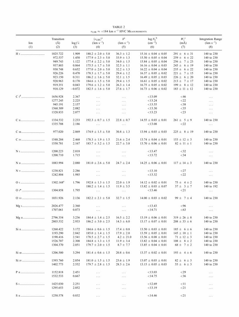
TABLE 2

vLSR � þ184 km s�1HVC Measurements

Ion

(1)

Transition

(8)(2)

log f k(3)

hvLSRia( km s�1)

(4)

ba

( km s�1)

(5)

logNab

(cm�2)

(6)

Wkc

(m8)(7)

Integration Range

(km s�1)

(8)

H i ............................... 1025.722 1.909 180.2 � 2.0 � 5.0 36.3 � 1.2 15.16 � 0.04 � 0.05 291 � 6 � 31 140 to 230

972.537 1.450 177.9 � 2.3 � 5.0 33.9 � 1.3 15.50 � 0.05 � 0.04 259 � 6 � 22 140 to 230

949.743 1.122 177.4 � 2.2 � 5.0 34.0 � 1.5 15.84 � 0.05 � 0.04 256 � 7 � 23 140 to 230

937.803 0.864 175.5 � 1.7 � 5.0 32.5 � 1.1 16.16 � 0.04 � 0.03 245 � 6 � 19 140 to 230

930.748 0.652 177.0 � 2.0 � 5.0 32.2 � 1.3 16.22 � 0.04 � 0.04 235 � 6 � 22 140 to 230

926.226 0.470 178.3 � 1.7 � 5.0 29.4 � 1.2 16.37 � 0.05 � 0.02 221 � 7 � 15 140 to 230

923.150 0.311 186.2 � 1.6 � 5.0 32.1 � 1.5 16.49 � 0.05 � 0.03 226 � 6 � 20 140 to 230

920.963 0.170 184.6 � 1.5 � 5.0 29.4 � 1.5 16.61 � 0.05 � 0.02 213 � 7 � 17 140 to 230

919.351 0.043 179.6 � 1.2 � 5.0 26.3 � 1.4 16.75 � 0.05 � 0.02 199 � 8 � 12 140 to 230

918.129 �0.072 182.5 � 1.6 � 5.0 27.6 � 1.7 16.73 � 0.06 � 0.02 183 � 11 � 12 140 to 230

C id .............................. 1656.928 2.367 . . . . . . <13.09 <46 . . .

1277.245 2.225 . . . . . . <13.24 <22 . . .945.191 2.157 . . . . . . <13.55 <38 . . .

1560.309 2.082 . . . . . . <13.30 <35 . . .

1328.833 2.077 . . . . . . <13.23 <23 . . .

C ii............................... 1334.532 2.233 192.3 � 0.7 � 1.5 22.8 � 0.7 14.55 � 0.03 � 0.01 261 � 5 � 9 140 to 230

1335.708 2.186 . . . . . . <13.08 <22 . . .

C iii.............................. 977.020 2.869 174.9 � 1.5 � 5.0 30.8 � 1.3 13.94 � 0.03 � 0.03 225 � 8 � 19 140 to 230

C iv.............................. 1548.204 2.468 178.3 � 1.9 � 1.5 21.6 � 2.4 13.74 � 0.04 � 0.01 153 � 12 � 3 140 to 230

1550.781 2.167 183.7 � 3.2 � 1.5 22.7 � 3.8 13.70 � 0.06 � 0.01 82 � 11 � 1 140 to 230

N i ............................... 1200.223 2.018 . . . . . . <13.47 <32 . . .

1200.710 1.715 . . . . . . <13.72 <34 . . .

N ii .............................. 1083.994 2.080 181.0 � 2.6 � 5.0 24.7 � 2.4 14.25 � 0.06 � 0.01 117 � 14 � 3 140 to 230

N v .............................. 1238.821 2.286 . . . . . . <13.10 <27 . . .1242.804 1.985 . . . . . . <13.32 <22 . . .

O i ............................... 1302.168e 1.796 192.8 � 1.3 � 1.5 22.0 � 1.9 14.12 � 0.02 � 0.01 75 � 4 � 2 140 to 230

180.2 � 1.4 � 1.5 11.9 � 3.5 13.82 � 0.03 � 0.07 37 � 3 � 7 140 to 192

O i* ............................. 1304.858 1.795 . . . . . . <13.46 <21 . . .

O vi ............................. 1031.926 2.136 182.2 � 2.1 � 5.0 32.7 � 1.5 14.00 � 0.03 � 0.02 99 � 7 � 4 140 to 230

Mg i............................. 2026.477 2.360 . . . . . . <13.43 <96 . . .

1707.061 0.873 . . . . . . <14.71 <63 . . .

Mg ii ............................ 2796.354 3.236 184.4 � 1.4 � 2.5 16.5 � 2.2 13.19 � 0.06 � 0.01 319 � 26 � 8 140 to 230

2803.532 2.933 186.2 � 3.0 � 2.5 14.3 � 6.0 13.17 � 0.07 � 0.01 208 � 33 � 6 140 to 230

Si ii .............................. 1260.422 3.172 184.6 � 0.6 � 1.5 17.4 � 0.8 13.50 � 0.03 � 0.01 185 � 6 � 6 140 to 230

1193.290 2.842 185.0 � 1.4 � 1.5 17.9 � 2.0 13.59 � 0.05 � 0.01 145 � 10 � 1 140 to 230

1190.416 2.541 178.5 � 2.7 � 1.5 4.2 � 21.0 13.56 � 0.08 � 0.01 71 � 12 � 3 140 to 230

1526.707 2.308 184.8 � 1.3 � 1.5 11.9 � 3.4 13.82 � 0.04 � 0.01 108 � 8 � 2 140 to 230

1304.370 2.051 179.7 � 2.0 � 1.5 8.7 � 7.7 13.85 � 0.04 � 0.01 68 � 7 � 2 140 to 230

Si iii ............................. 1206.500 3.294 181.4 � 0.6 � 1.5 20.8 � 0.6 13.37 � 0.02 � 0.01 193 � 4 � 6 140 to 230

Si iv ............................. 1393.760 2.854 181.0 � 1.5 � 1.5 23.6 � 1.9 13.07 � 0.03 � 0.01 82 � 6 � 3 140 to 230

1402.773 2.552 179.7 � 2.8 � 1.5 28.3 � 2.6 13.15 � 0.05 � 0.03 55 � 6 � 3 140 to 230

P ii ............................... 1152.818 2.451 . . . . . . <13.03 <29 . . .1532.533 0.667 . . . . . . <14.75 <36 . . .

S i ................................ 1425.030 2.251 . . . . . . <12.69 <11 . . .

1295.653 2.052 . . . . . . <13.19 <21 . . .

S ii ............................... 1250.578 0.832 . . . . . . <14.46 <21 . . .

profiles is to first resample the individual ACD profiles (and theirrespective error vectors) to common velocity bins using a cubicspline interpolation (Press et al.1992) and then perform a variance-weighted average for each velocity bin of the apparent columndensities from optically thin transitions (i.e., where the apparentoptical depth, �aðv iÞ ¼ ln ½1=Iðv iÞ� < 1). In cases where all tran-sitions are optically thick, we use the 1 � lower limit from theweakest transition. FUSE data are not used in the compositeprofiles since the resolution of spectra are much poorer thanthe STIS spectra. In cases where E230M data are combined, weresample the ACD profiles to 5 km s�1 bins. When E140M dataare combined, we resample the ACD profiles to 3.5 km s�1 bins.Our primary purpose in creating composites is for line shapecomparisons in the vLSR � þ184 km s�1 HVC, not for columndensity measurements. As such, we do not require a detailedevaluation of the propagation of errors through the resamplingprocedure. We have verified through visual inspection that thecomposites provide a good facsimile of the underlying apparentcolumn density profiles.

In the Appendix, we discuss the details of the transitionschosen for each ion for the composite ACD computation and forthe adopted variance-weighted mean integrated apparent col-umn density reported in Table 4. The final composite NaðvÞprofiles for ions detected in Galactic absorption are shown inFigure 4. H i was not included in this computation because thehigher order Lyman series lines detected in the FUSE band arestrong and suffer from blends with other lines. We return tomeasurements of the H i profiles below.

5. LOW- AND INTERMEDIATE-VELOCITY GAS

High-ionization gas traced by Si iv, C iv, N v, and O vi iscommon along high-latitude sight lines that extend severalkiloparsecs or more through the Galactic thick disk and halo.PG 1116+215 lies in a region of the sky well above the influenceof spiral arm structure and outside nearby radio loops that maycontribute to some of the high-ionization gas (Sembach et al.1997). Most of the high-ionization gas at low velocities towardPG 1116+215 occurs in the thick disk/halo because the high

latitude of the sight line (b ¼ 68N21) ensures that only tenuousgas in the solar neighborhood is intercepted within 100 pc ofthe Galactic disk. The amount of O vi expected within�100 pcof the Sun is P1013 cm�2 (Oegerle et al. 2005), or P8% of thetotal observed in the �44, �7, and +56 km s�1 components.The sight line therefore allows an examination of the high ioncolumn density ratios in gas associated predominantly with thethick disk/halo of the Galaxy.

The amount of O vi observed in the Milky Way thick-disk/halo toward PG 1116+215 over the velocity range from�100 to+85 km s�1, log N(O vi) = 14.16 (see Table 3), is typical of thatexpected for a plane-parallel gas layer with an exponential den-sity distribution, an O vi scale height of 2.3 kpc, a midplane den-sity n0ðO viÞ � 1:7 ; 10�8 cm�3, and a �0.25 dex enhancementas seen along high-latitude sight lines in the northern Galactichemisphere (Savage et al. 2003). The other high ions also havetotal column densities in the low- and intermediate-velocitycomponents that are typical for extragalactic sight lines; we findlog NðC ivÞ ¼ 14:17, log NðN vÞ < 13:14, and logNðSi ivÞ ¼13:69 in the�100 km s�1� vLSR � þ85 km s�1 velocity range.

The thick disk/halo absorption toward PG 1116+215 consistsof three separate low-ionization components with continuousabsorption in the high-ionization species over the velocity range�100 km s�1 PvLSR P þ 85 km s�1. At these velocities, theC iv and Si iv profiles are quite similar, with average columndensity weighted centroids of �13 and ��15 km s�1, respec-tively (see Table 3). The widths of the absorption features arealso similar, with the C iv lines being slightly broader: bðC ivÞ �60 km s�1 and bðSi ivÞ � 45 km s�1. The centroids of the C iv

and Si iv are significantly different from the O vi centroid,hvi �þ18 km s�1, indicating that there are important differencesin the distributions of these two ions and the distribution of thelow-velocity O vi. Most of this difference arises from the lack ofsubstantial O vi in the �44 km s�1 component [logNðO viÞ <13:24; see Fig. 4 and Table 4]. It is noteworthy that this isthe only component along the sight line that contains detect-able H2 absorption. Most IVCs are within 1 kpc of the Galac-tic disk (Wakker 2001), so this component is probably closer

TABLE 2—Continued

Ion

(1)

Transition

(8)(2)

log f k(3)

hvLSRia(km s�1)

(4)

ba

(km s�1)

(5)

log Nab

(cm�2)

(6)

Wkc

(m8)(7)

Integration Range

(km s�1)

(8)

Fe ii .................................... 2382.765 2.882 185.5 � 1.4 � 2.5 20.0 � 2.0 13.41 � 0.04 � 0.01 240 � 18 � 4 140 to 230

2600.173 2.793 182.7 � 1.4 � 2.5 14.8 � 2.9 13.41 � 0.05 � 0.01 186 � 18 � 11 140 to 230

2344.214 2.427 . . . . . . 13.36 � 0.09 � 0.02 92 � 22 � 7 140 to 230

2586.650 2.252 . . . . . . 13.47 � 0.10 � 0.03 88 � 23 � 9 140 to 230

1608.451 1.968 . . . . . . <13.49 <39 . . .

2374.461 1.871 . . . . . . <13.70 <71 . . .

2260.780 0.742 . . . . . . <14.73 <63 . . .

2249.877 0.612 . . . . . . <14.73 <45 . . .

Notes.—Uncertainties on measured values are reported at 1 � confidence. For integrated apparent column densities and equivalent widths, two uncertainties arequoted. The first is the estimated 1 � uncertainty from the quadrature addition of statistical and continuum placement errors. The second is the uncertainty resulting fromchanging the width of the integration range by 10 km s�1.

a Velocity centroids and b-values are derived using the apparent optical depth method (see eq. [3]) and are reported only if the equivalent width exceeds 5 times itserror. The second errors quoted for the velocity centroid reflect the uncertainty in the absolute wavelength calibration (�5 km s�1 for FUSE,�1.5 km s�1 for E140M, and�2.5 km s�1 for E230M). These do not affect the measurements of b-values, since those constitute differential measurements about the centroid.

b Apparent column density upper limits are 3 � confidence estimates derived from direct integration over the integration range 140–230 km s�1.c Equivalent width limits are 3 � confidence estimates over the integration range 140–230 km s�1.d For the 1277.245, 1328.833, and 1656.928 8 lines, we adopt the self-consistent values of f k derived by Jenkins & Tripp (2001).e Two entries are listed for the O i k1302.169 transition corresponding to two chosen integration ranges. The HVC profile appears to be blended with an unrelated

absorption feature redward of the HVC. This feature may be a weak intergalactic Ly� absorption line at z � 0:0719 (see Sembach et al. 2004a). The first row includesthis feature in the integration, while the second row limits the integration to exclude the feature (cutting off the integration at vLSR ¼ þ192 km s�1). See x 7.2.1 for adetailed examination of the O i column density for this HVC.


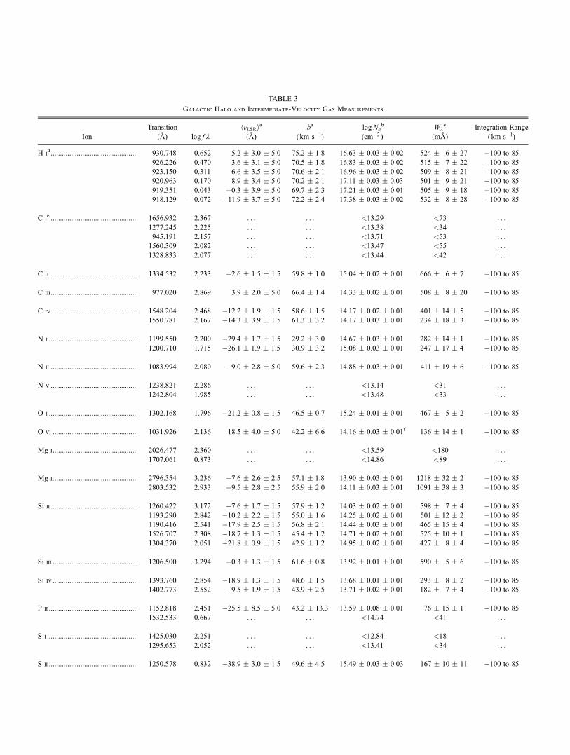
TABLE 3

Galactic Halo and Intermediate-Velocity Gas Measurements

Ion

Transition

(8) log f khvLSRia(8)

ba

( km s�1)

logNab

(cm�2 )

Wkc

(m8)Integration Range

(km s�1)

H id.............................................. 930.748 0.652 5.2 � 3.0 � 5.0 75.2 � 1.8 16.63 � 0.03 � 0.02 524 � 6 � 27 �100 to 85

926.226 0.470 3.6 � 3.1 � 5.0 70.5 � 1.8 16.83 � 0.03 � 0.02 515 � 7 � 22 �100 to 85

923.150 0.311 6.6 � 3.5 � 5.0 70.6 � 2.1 16.96 � 0.03 � 0.02 509 � 8 � 21 �100 to 85

920.963 0.170 8.9 � 3.4 � 5.0 70.2 � 2.1 17.11 � 0.03 � 0.03 501 � 9 � 21 �100 to 85

919.351 0.043 �0.3 � 3.9 � 5.0 69.7 � 2.3 17.21 � 0.03 � 0.01 505 � 9 � 18 �100 to 85

918.129 �0.072 �11.9 � 3.7 � 5.0 72.2 � 2.4 17.38 � 0.03 � 0.02 532 � 8 � 28 �100 to 85

C ie .............................................. 1656.932 2.367 . . . . . . <13.29 <73 . . .

1277.245 2.225 . . . . . . <13.38 <34 . . .

945.191 2.157 . . . . . . <13.71 <53 . . .1560.309 2.082 . . . . . . <13.47 <55 . . .

1328.833 2.077 . . . . . . <13.44 <42 . . .

C ii............................................... 1334.532 2.233 �2.6 � 1.5 � 1.5 59.8 � 1.0 15.04 � 0.02 � 0.01 666 � 6 � 7 �100 to 85

C iii.............................................. 977.020 2.869 3.9 � 2.0 � 5.0 66.4 � 1.4 14.33 � 0.02 � 0.01 508 � 8 � 20 �100 to 85

C iv.............................................. 1548.204 2.468 �12.2 � 1.9 � 1.5 58.6 � 1.5 14.17 � 0.02 � 0.01 401 � 14 � 5 �100 to 85

1550.781 2.167 �14.3 � 3.9 � 1.5 61.3 � 3.2 14.17 � 0.03 � 0.01 234 � 18 � 3 �100 to 85

N i ............................................... 1199.550 2.200 �29.4 � 1.7 � 1.5 29.2 � 3.0 14.67 � 0.03 � 0.01 282 � 14 � 1 �100 to 85

1200.710 1.715 �26.1 � 1.9 � 1.5 30.9 � 3.2 15.08 � 0.03 � 0.01 247 � 17 � 4 �100 to 85

N ii .............................................. 1083.994 2.080 �9.0 � 2.8 � 5.0 59.6 � 2.3 14.88 � 0.03 � 0.01 411 � 19 � 6 �100 to 85

N v .............................................. 1238.821 2.286 . . . . . . <13.14 <31 . . .

1242.804 1.985 . . . . . . <13.48 <33 . . .

O i ............................................... 1302.168 1.796 �21.2 � 0.8 � 1.5 46.5 � 0.7 15.24 � 0.01 � 0.01 467 � 5 � 2 �100 to 85

O vi ............................................. 1031.926 2.136 18.5 � 4.0 � 5.0 42.2 � 6.6 14.16 � 0.03 � 0.01f 136 � 14 � 1 �100 to 85

Mg i............................................. 2026.477 2.360 . . . . . . <13.59 <180 . . .

1707.061 0.873 . . . . . . <14.86 <89 . . .

Mg ii ............................................ 2796.354 3.236 �7.6 � 2.6 � 2.5 57.1 � 1.8 13.90 � 0.03 � 0.01 1218 � 32 � 2 �100 to 85

2803.532 2.933 �9.5 � 2.8 � 2.5 55.9 � 2.0 14.11 � 0.03 � 0.01 1091 � 38 � 3 �100 to 85

Si ii .............................................. 1260.422 3.172 �7.6 � 1.7 � 1.5 57.9 � 1.2 14.03 � 0.02 � 0.01 598 � 7 � 4 �100 to 85

1193.290 2.842 �10.2 � 2.2 � 1.5 55.0 � 1.6 14.25 � 0.02 � 0.01 501 � 12 � 2 �100 to 85

1190.416 2.541 �17.9 � 2.5 � 1.5 56.8 � 2.1 14.44 � 0.03 � 0.01 465 � 15 � 4 �100 to 85

1526.707 2.308 �18.7 � 1.3 � 1.5 45.4 � 1.2 14.71 � 0.02 � 0.01 525 � 10 � 1 �100 to 85

1304.370 2.051 �21.8 � 0.9 � 1.5 42.9 � 1.2 14.95 � 0.02 � 0.01 427 � 8 � 4 �100 to 85

Si iii ............................................. 1206.500 3.294 �0.3 � 1.3 � 1.5 61.6 � 0.8 13.92 � 0.01 � 0.01 590 � 5 � 6 �100 to 85

Si iv ............................................. 1393.760 2.854 �18.9 � 1.3 � 1.5 48.6 � 1.5 13.68 � 0.01 � 0.01 293 � 8 � 2 �100 to 85

1402.773 2.552 �9.5 � 1.9 � 1.5 43.9 � 2.5 13.71 � 0.02 � 0.01 182 � 7 � 4 �100 to 85

P ii ............................................... 1152.818 2.451 �25.5 � 8.5 � 5.0 43.2 � 13.3 13.59 � 0.08 � 0.01 76 � 15 � 1 �100 to 85

1532.533 0.667 . . . . . . <14.74 <41 . . .

S i ................................................ 1425.030 2.251 . . . . . . <12.84 <18 . . .

1295.653 2.052 . . . . . . <13.41 <34 . . .

S ii ............................................... 1250.578 0.832 �38.9 � 3.0 � 1.5 49.6 � 4.5 15.49 � 0.03 � 0.03 167 � 10 � 11 �100 to 85

than some of the other low-velocity Si iv and C iv absorptionfeatures.

Strong low-ionization features, such as C ii k1334.532, havea negative velocity absorption cutoff at essentially the samevelocity as C iv or Si iv (vLSR ��90 km s�1). This indicates thatthe high- and low-ionization species in the�44 km s�1 IVC areclosely coupled kinematically and, by inference, spatially. Theintermediate-ionization C iii k977.020 line closely approx-imates this behavior as well; its great strength suggests thatthere may be a small amount of gas at slightly more negativevelocities. The column density ratio of NðC ivÞ=NðSi ivÞ � 3in this component is typical of that for clouds in the generalinterstellar medium (see Sembach et al. 1997). Savage et al.(1994) have suggested that the constancy of the C iv-to-Si ivratio along many different directions through the Galactic diskand low halo can be attributed to regulation of the ionization byconductive interfaces, a result born out by their high-resolutionGHRS data that shows a close kinematical relationship betweenthe high ions and lower ionization velocity components alongthe HD 167756 sight line. The same ratio of �3 is found in theother low- and intermediate-velocity features toward PG 1116+215 as well. The upper limits on N v and O vi in the�44 km s�1

component place limits on the age of the conduction front. Thepredicted strength of O vi is generally less than that of C iv forconduction front ages P105 yr (Borkowski et al. 1990). Thus, ifconduction is important in regulating the Si iv and C iv columndensities in this component, the front must be in an early stageof evolution.

The ionization of the Galactic thick disk and halo gas towardPG 1116+215 is likely a hybrid of different collisional ioniza-tion processes as no single model seems to be able to explain thehigh ion column density ratios in all of the observed compo-nents. We list the observed ratios of Si iv, C iv, and N v to O vi

in Table 5 together with the corresponding ratios predicted fordifferent ionization mechanisms. The sources of the theoreticalmodel predictions are listed in the footnotes of Table 5 as well asthe ranges of model parameters considered in computing thecolumn density ratios. All values listed are appropriate for solar

abundance gas, which should be a reasonable approximationfor the thick disk/halo and IVC components considered here.Previous studies have shown that multiple ionization mecha-nisms are required to explain the total high ion column densityratios along sight lines through the halo (e.g., Sembach &Savage 1992; Savage et al. 1997, 2003; Indebetouw & Shull2004), and PG 1116+215 is no exception. This is not surprisinggiven the range of ion ratios observed in the three components.For example, both the Si iv/O vi and C iv/O vi column densityratios differ dramatically between the two components at �44and �7 km s�1, while the C iv/Si iv ratio is �3 in both cases.Apparently, the high-ionization gas is sufficiently complex thatno single process dominates the observed ionization signatureof the Galactic disk and halo gas along the sight line.

6. HIGH-VELOCITY GAS AT vLSR � þ100 km s�1

As described in x 3, there are clear signs of a high-velocitycloud at vLSR � þ100 km s�1. A discrete feature at this velocitycan be seen in the profiles of C ii, Si ii (in the 1260.422 8 line),and Si iii. The gas is not detected in any neutral ions covered bythe spectra; there are no indications of significant column den-sities in C i, N i, or O i. Likewise, the cloud is not detected inany singly ionized species other than C ii and Si ii; there is nosignificant column density in N ii, Mg ii, P ii, S ii, or Fe ii.Absorption in the C iii 977.020 8 line is also present, but it isaffected by unresolved saturation. There is significant columndensity at vLSR � þ100 km s�1 in the higher ionization species,but it is difficult to associate the high-ionization gas with thiscomponent for two reasons: (1) the kinematics of the high-ionization species is peaked at the vLSR � þ184 km s�1 HVCwith a trailing absorption wing extending down to this velocity(see x 7); and (2) the (nonzero) minimum in the apparent col-umn density profiles occurs near this velocity. For this reason,the column densities of high-ionization species listed in Table 1for this component should be treated with care in the interpre-tation of the ionization of this gas.

It is interesting to note that the +100 km s�1 HVC has prop-erties that are quite similar to those of an intergalactic gas cloud

TABLE 3—Continued

Ion

Transition

(8) log f khvLSRia(8)

ba

( km s�1)

logNab

(cm�2 )

Wkc

(m8)Integration Range

(km s�1)

Fe ii .......................................... 2382.765 2.882 �12.4 � 2.2 � 2.5 55.7 � 1.6 14.13 � 0.02 � 0.01 924 � 23 � 3 �100 to 85

2600.173 2.793 �13.3 � 1.7 � 2.5 51.7 � 1.4 14.22 � 0.02 � 0.01 966 � 23 � 10 �100 to 85

2344.214 2.427 �21.2 � 1.7 � 2.5 42.0 � 1.9 14.55 � 0.03 � 0.01 760 � 28 � 3 �100 to 85

2586.650 2.252 �23.9 � 1.9 � 2.5 38.6 � 2.3 14.61 � 0.04 � 0.01 689 � 29 � 6 �100 to 85

1608.451 1.968 �27.5 � 1.8 � 1.5 40.1 � 2.6 14.79 � 0.03 � 0.01 373 � 16 � 2 �100 to 85

2374.461 1.871 �28.4 � 2.2 � 2.5 40.8 � 3.3 14.86 � 0.03 � 0.01 513 � 30 � 7 �100 to 85

2260.780 0.742 �21.1 � 7.9 � 2.5 44.5 � 12.0 15.16 � 0.06 � 0.01 134 � 23 � 3 �100 to 85

2249.877 0.612 . . . . . . 15.04 � 0.11 � 0.03 73 � 24 � 5 �100 to 85

Notes.—Uncertainties on measured values are reported at 1 � confidence. For integrated apparent column densities and equivalent widths, two uncertainties arequoted. The first is the estimated 1 � uncertainty from the quadrature addition of statistical and continuum placement errors. The second is the uncertainty resulting fromchanging the width of the integration range by 10 km s�1.

a Velocity centroids and b-values are derived using the apparent optical depth method (see eq. [3]) and are reported only if the equivalent width exceeds 5 times itserror. The second errors quoted for the velocity centroid reflect the uncertainty in the absolute wavelength calibration (�5 km s�1 for FUSE,�1.5 km s�1 for E140M, and�2.5 km s�1 for E230M). These do not affect the measurements of b-values, since those constitute differential measurements about the centroid.

b Apparent column density upper limits are 3 � confidence estimates derived from direct integration over the integration range �100 to +85 km s�1.c Equivalent width limits are reported to 3 � confidence over the integration range �100 to +85 km s�1.d The Ly�–Ly� absorption lines at low velocities are contaminated by geocoronal emission. Consequently, we do not present measurements of these lines.

Moreover, the apparent increases in the equivalent widths of the Ly� (919.351 8) and Lyk (918.129 8) lines are due to blends in the region of the high-order Lymanseries with higher order Lyman series absorption, high-velocity Lyman series absorption features, and O i absorption.

e For the 1277.245, 1328.833, and 1656.928 8 lines, we adopt the self-consistent values of f k derived by Jenkins & Tripp (2001).f We note that Savage et al. (2003) find logNðO viÞ ¼ 14:26 � 0:03 over the velocity range �55 to +115 km s�1, which agrees well with the listed value if the

column density of the +100 km s�1 component listed in Table 1 is included with our estimate.


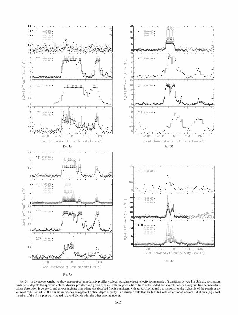
Fig. 3aFig. 3bFig. 3cFig. 3d

Fig. 3.—In the above panels, we show apparent column density profiles vs. local standard of rest velocity for a sample of transitions detected in Galactic absorption.Each panel depicts the apparent column density profiles for a given species, with the profile transitions color-coded and overplotted. A histogram line connects binswhere absorption is detected, and arrows indicate bins where the absorbed flux is consistent with zero. A horizontal bar is shown on the right side of the panels at thevalue of NaðvÞ for which the transition reaches an apparent optical depth of unity. For clarity, pixels that are blended with other transitions are not shown (e.g., eachmember of the N i triplet was cleaned to avoid blends with the other two members).

Fig. 3a Fig. 3b

Fig. 3c

Fig. 3d

262

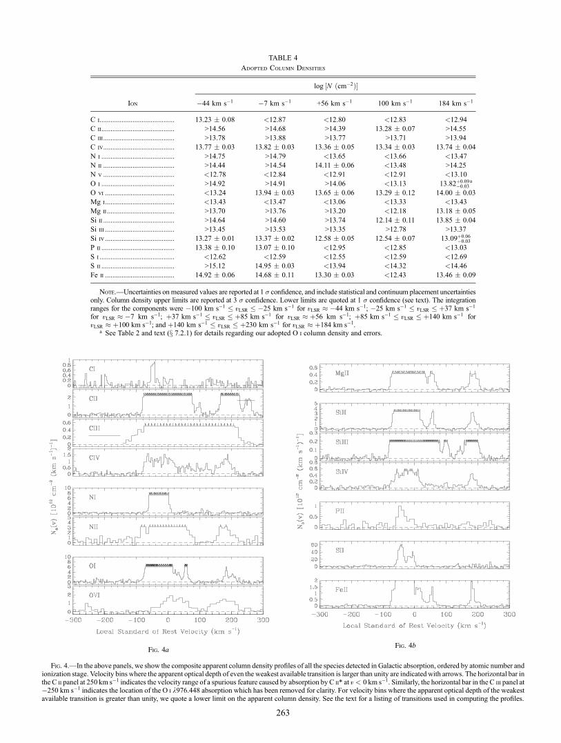
TABLE 4

Adopted Column Densities

log ½N ðcm�2Þ�

Ion �44 km s�1 �7 km s�1 +56 km s�1 100 km s�1 184 km s�1

C i......................................... 13.23 � 0.08 <12.87 <12.80 <12.83 <12.94

C ii........................................ >14.56 >14.68 >14.39 13.28 � 0.07 >14.55

C iii....................................... >13.78 >13.88 >13.77 >13.71 >13.94

C iv....................................... 13.77 � 0.03 13.82 � 0.03 13.36 � 0.05 13.34 � 0.03 13.74 � 0.04

N i ........................................ >14.75 >14.79 <13.65 <13.66 <13.47

N ii ....................................... >14.44 >14.54 14.11 � 0.06 <13.48 >14.25

N v ....................................... <12.78 <12.84 <12.91 <12.91 <13.10

O i ........................................ >14.92 >14.91 >14.06 <13.13 13:82þ0:09�0:03

a

O vi ...................................... <13.24 13.94 � 0.03 13.65 � 0.06 13.29 � 0.12 14.00 � 0.03

Mg i...................................... <13.43 <13.47 <13.06 <13.33 <13.43

Mg ii ..................................... >13.70 >13.76 >13.20 <12.18 13.18 � 0.05

Si ii ....................................... >14.64 >14.60 >13.74 12.14 � 0.11 13.85 � 0.04

Si iii ...................................... >13.45 >13.53 >13.35 >12.78 >13.37

Si iv ...................................... 13.27 � 0.01 13.37 � 0.02 12.58 � 0.05 12.54 � 0.07 13:09þ0:06�0:03

P ii ........................................ 13.38 � 0.10 13.07 � 0.10 <12.95 <12.85 <13.03

S i ......................................... <12.62 <12.59 <12.55 <12.59 <12.69

S ii ........................................ >15.12 14.95 � 0.03 <13.94 <14.32 <14.46

Fe ii ...................................... 14.92 � 0.06 14.68 � 0.11 13.30 � 0.03 <12.43 13.46 � 0.09

Note.—Uncertainties on measured values are reported at 1 � confidence, and include statistical and continuum placement uncertaintiesonly. Column density upper limits are reported at 3 � confidence. Lower limits are quoted at 1 � confidence (see text). The integrationranges for the components were �100 km s�1 � vLSR � �25 km s�1 for vLSR � �44 km s�1; �25 km s�1 � vLSR � þ37 km s�1

for vLSR � �7 km s�1; þ37 km s�1 � vLSR � þ85 km s�1 for vLSR � þ56 km s�1; þ85 km s�1 � vLSR � þ140 km s�1 forvLSR � þ100 km s�1; and þ140 km s�1 � vLSR � þ230 km s�1 for vLSR � þ184 km s�1.

a See Table 2 and text (x 7.2.1) for details regarding our adopted O i column density and errors.

Fig. 4aFig. 4b

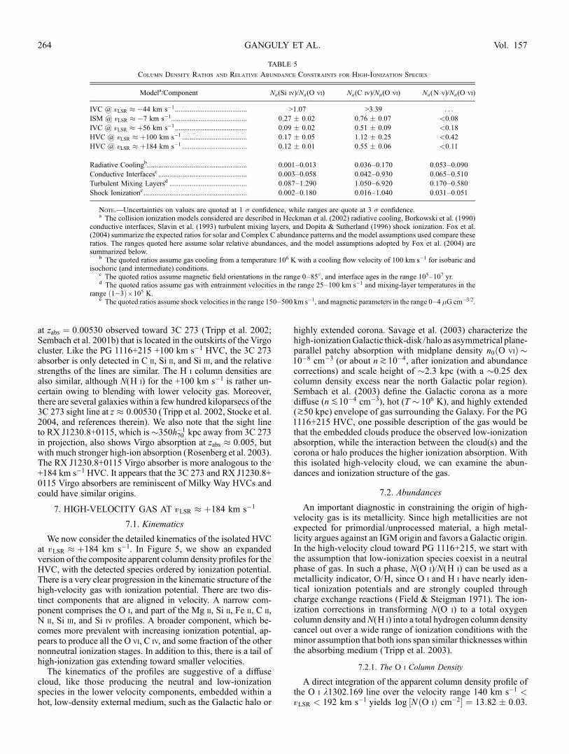
Fig. 4.—In the above panels, we show the composite apparent column density profiles of all the species detected in Galactic absorption, ordered by atomic number andionization stage. Velocity bins where the apparent optical depth of even the weakest available transition is larger than unity are indicated with arrows. The horizontal bar inthe C ii panel at 250 km s�1 indicates the velocity range of a spurious feature caused by absorption by C ii* at v < 0 km s�1. Similarly, the horizontal bar in the C iii panel at�250 km s�1 indicates the location of the O i k976.448 absorption which has been removed for clarity. For velocity bins where the apparent optical depth of the weakestavailable transition is greater than unity, we quote a lower limit on the apparent column density. See the text for a listing of transitions used in computing the profiles.

Fig. 4aFig. 4b

263

at zabs ¼ 0:00530 observed toward 3C 273 (Tripp et al. 2002;Sembach et al. 2001b) that is located in the outskirts of the Virgocluster. Like the PG 1116+215 +100 km s�1 HVC, the 3C 273absorber is only detected in C ii, Si ii, and Si iii, and the relativestrengths of the lines are similar. The H i column densities arealso similar, although N(H i) for the +100 km s�1 is rather un-certain owing to blending with lower velocity gas. Moreover,there are several galaxies within a few hundred kiloparsecs of the3C 273 sight line at z � 0:00530 (Tripp et al. 2002, Stocke et al.2004, and references therein). We also note that the sight lineto RX J1230.8+0115, which is�350h�1

70 kpc away from 3C 273in projection, also shows Virgo absorption at zabs � 0:005, butwith much stronger high-ion absorption (Rosenberg et al. 2003).The RX J1230.8+0115 Virgo absorber is more analogous to the+184 km s�1 HVC. It appears that the 3C 273 and RX J1230.8+0115 Virgo absorbers are reminiscent of Milky Way HVCs andcould have similar origins.

7. HIGH-VELOCITY GAS AT vLSR � þ184 km s�1

7.1. Kinematics

We now consider the detailed kinematics of the isolated HVCat vLSR � þ184 km s�1. In Figure 5, we show an expandedversion of the composite apparent column density profiles for theHVC, with the detected species ordered by ionization potential.There is a very clear progression in the kinematic structure of thehigh-velocity gas with ionization potential. There are two dis-tinct components that are aligned in velocity. A narrow com-ponent comprises the O i, and part of the Mg ii, Si ii, Fe ii, C ii,N ii, Si iii, and Si iv profiles. A broader component, which be-comes more prevalent with increasing ionization potential, ap-pears to produce all the O vi, C iv, and some fraction of the othernonneutral ionization stages. In addition to this, there is a tail ofhigh-ionization gas extending toward smaller velocities.

The kinematics of the profiles are suggestive of a diffusecloud, like those producing the neutral and low-ionizationspecies in the lower velocity components, embedded within ahot, low-density external medium, such as the Galactic halo or

highly extended corona. Savage et al. (2003) characterize thehigh-ionizationGalactic thick-disk/halo as asymmetrical plane-parallel patchy absorption with midplane density n0ðO viÞ �10�8 cm�3 (or about nk10�4, after ionization and abundancecorrections) and scale height of �2.3 kpc (with a �0.25 dexcolumn density excess near the north Galactic polar region).Sembach et al. (2003) define the Galactic corona as a morediffuse (nP10�4 cm�3), hot (T � 106 K), and highly extended(k50 kpc) envelope of gas surrounding the Galaxy. For the PG1116+215 HVC, one possible description of the gas would bethat the embedded clouds produce the observed low-ionizationabsorption, while the interaction between the cloud(s) and thecorona or halo produces the higher ionization absorption. Withthis isolated high-velocity cloud, we can examine the abun-dances and ionization structure of the gas.

7.2. Abundances

An important diagnostic in constraining the origin of high-velocity gas is its metallicity. Since high metallicities are notexpected for primordial /unprocessed material, a high metal-licity argues against an IGM origin and favors a Galactic origin.In the high-velocity cloud toward PG 1116+215, we start withthe assumption that low-ionization species coexist in a neutralphase of gas. In such a phase, N(O i)/N(H i) can be used as ametallicity indicator, O/H, since O i and H i have nearly iden-tical ionization potentials and are strongly coupled throughcharge exchange reactions (Field & Steigman 1971). The ion-ization corrections in transforming N(O i) to a total oxygencolumn density andN(H i) into a total hydrogen column densitycancel out over a wide range of ionization conditions with theminor assumption that both ions span similar thicknesses withinthe absorbing medium (Tripp et al. 2003).

7.2.1. The O i Column Density

A direct integration of the apparent column density profile ofthe O i k1302.169 line over the velocity range 140 km s�1 <vLSR < 192 km s�1 yields log ½NðO iÞ cm�2� ¼ 13:82 � 0:03.

TABLE 5

Column Density Ratios and Relative Abundance Constraints for High-Ionization Species

Modela/Component Na(Si iv)/Na(O vi) Na(C iv)/Na(O vi) Na(N v)/Na(O vi)

IVC @ vLSR � �44 km s�1....................................... >1.07 >3.39 . . .

ISM @ vLSR � �7 km s�1......................................... 0.27 � 0.02 0.76 � 0.07 <0.08

IVC @ vLSR � þ56 km s�1....................................... 0.09 � 0.02 0.51 � 0.09 <0.18

HVC @ vLSR � þ100 km s�1 ................................... 0.17 � 0.05 1.12 � 0.25 <0.42

HVC @ vLSR � þ184 km s�1 ................................... 0.12 � 0.01 0.55 � 0.06 <0.11

Radiative Coolingb...................................................... 0.001–0.013 0.036–0.170 0.053–0.090

Conductive Interfacesc ................................................ 0.003–0.058 0.042–0.930 0.065–0.510

Turbulent Mixing Layersd .......................................... 0.087–1.290 1.050–6.920 0.170–0.580

Shock Ionizatione........................................................ 0.002–0.180 0.016–1.040 0.031–0.051

Note.—Uncertainties on values are quoted at 1 � confidence, while ranges are quote at 3 � confidence.a The collision ionization models considered are described in Heckman et al. (2002) radiative cooling, Borkowski et al. (1990)

conductive interfaces, Slavin et al. (1993) turbulent mixing layers, and Dopita & Sutherland (1996) shock ionization. Fox et al.(2004) summarize the expected ratios for solar and Complex C abundance patterns and the model assumptions used compare theseratios. The ranges quoted here assume solar relative abundances, and the model assumptions adopted by Fox et al. (2004) aresummarized below.

b The quoted ratios assume gas cooling from a temperature 106 K with a cooling flow velocity of 100 km s�1 for isobaric andisochoric (and intermediate) conditions.

c The quoted ratios assume magnetic field orientations in the range 0–85�, and interface ages in the range 105–107 yr.d The quoted ratios assume gas with entrainment velocities in the range 25–100 km s�1 and mixing-layer temperatures in the

range ð1 3Þ ; 105 K.e The quoted ratios assume shock velocities in the range 150–500 km s�1, and magnetic parameters in the range 0–4 G cm�3/2.


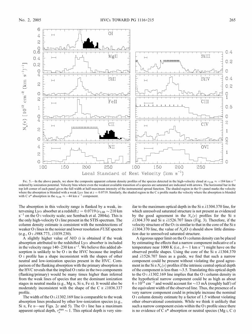
The absorption in this velocity range is flanked by a weak, in-tervening Ly� absorber at a redshift z ¼ 0:0719 (vLSR � 210 kms�1 on the O i velocity scale; see Sembach et al. 2004a). This isthe only high-velocity O i line present in the STIS spectrum. Thecolumn density estimate is consistent with the nondetections ofweaker O i lines in the noisier and lower resolution FUSE spectra(e.g., O i k988.773, k1039.230).

A slightly higher value of N(O i) is obtained if the weakabsorption attributed to the redshifted Ly� absorber is includedin the velocity range 140–230 km s�1. We believe this added ab-sorption is unlikely to be O i in the HVC because the impliedO i profile has a shape inconsistent with the shapes of otherneutral and low-ionization species present in the HVC. Com-parison of the flanking absorption with the primary absorption inthe HVC reveals that the implied O i ratio in the two components(flanking/primary) would be many times higher than inferredfrom the weak lines of species that are the dominant ionizationstages in neutral media (e.g., Mg ii, Si ii, Fe ii). It would also bemoderately inconsistent with the shape of the C ii k1036.337profile.

The width of the O i k1302.169 line is comparable to the weakabsorption lines produced by other low-ionization species (e.g.,Si ii, Fe ii—see Figs. 2c and 5). The O i line has a maximumapparent optical depth, �max

a � 1. This optical depth is very sim-

ilar to the maximum optical depth in the Si ii k1304.370 line, forwhich unresolved saturated structure is not present as evidencedby the good agreement in the NaðvÞ profiles for the Si ii

k1304.370 and Si ii k1526.707 lines (Fig. 3). Therefore, if thevelocity structure of the O i is similar to that in the core of the Si iik1304.370 line, the value of Na(O i) should show little diminu-tion due to unresolved saturated structure.

A rigorous upper limit on the O i column density can be placedby estimating the effects that a narrow component indicative of atemperature near 1000 K (i.e., b� 1 km s�1) might have on theobserved profile shapes. Using the core of the Si ii k1304.370and k1526.707 lines as a guide, we find that such a narrowcomponent could be present without violating the good agree-ment in the Si iiNaðvÞ profiles if the intrinsic central optical depthof the component is less than�3.5. Translating this optical depthto the O i k1302.169 line implies that the O i column density inthe hypothetical narrow component could be as high as about6 ; 1014 cm�2 and would account for�13 m8 (roughly half ) ofthe equivalent width of the observed line. Thus, the presence of avery narrow component could in principle increase the nominalO i column density estimate by a factor of 1.5 without violatingother observational constraints. While we think it unlikely thatsuch a narrow component exists within the O i profile since thereis no evidence of C ii* absorption or neutral species (Mg i, C i)

Fig. 5.—In the above panels, we show the composite apparent column density profiles of the species detected in the high-velocity cloud at vLSR � þ184 km s�1

ordered by ionization potential. Velocity bins where even the weakest available transition of a species are saturated are indicated with arrows. The horizontal bar in thetop left corner of each panel gives the full width at half-maximum intensity of the instrumental spread function. The shaded region in the O i panel marks the velocitywhere the absorption is blended with a weak Ly� line at z ¼ 0:0719. Similarly, the shaded region in the C ii profile marks the velocity where the absorption is blendedwith C ii* absorption in the vLSR � �44 km s�1 component.

HVCs TOWARD PG 1116+215 265No. 2, 2005

that would favor its presence, we nevertheless adopt a conser-vative logarithmic O i column density range of 13.79–13.91, orlog NðO iÞ ¼ 13:82þ0:09

�0:03 in our discussions of the O i columndensity below. This value is reported in Table 4.

7.2.2. The H i Column Density

From the direct integration of the H i Lyk line in the FUSEspectrum, and the nondetection of the H i 21 cm emission fromWakker et al. (2003), the HVCH i column density must lie in therange ð5:2 200Þ ; 1016 cm�2. To further constrain this range, wetake two approaches to measuring the H i column density—profile-fitting the higher order Lyman series, and a curve ofgrowth fit to the H i equivalent widths reported in Table 2.

In our first approach, we have attempted to fit the higher orderLyman series detected in the FUSE spectrum. Since the higherorder Lyman series lines of the vLSR � þ184 km s�1 HVC areblended with both the H i lines from intermediate-velocity andGalactic absorption, and with several O i transitions, we firstconsidered the available constraints on the kinematics, columndensities, and intrinsic line widths from these lines prior to thefitting the H i profile of the HVC. In our consideration, it is onlyimportant to construct a model which accurately reproduces theshapes of the absorption profiles. Consequently, in constructingthe model, we started with the information already provided bythe H i 21 cm emission profiles from Wakker et al. (2003), thehigh-velocity O i column density derived above, and the kine-matic information for the low-ionization lines from x 3. Thus,our model contains five kinematic components at velocitiesvLSR � �44,�7, +56, +100, and +184 km s�1. From a fit to theH i 21 cm emission, Wakker et al. (2003) report H i columndensities of 1019.83 and 1019.70 cm�2, and b-values of 15.5 and14.7 km s�1 for the vLSR � �44 km s�1 and vLSR � �7 km s�1

components, respectively. To further reduce the number of freeparameters, we fixed the O i column densities of these twocomponents to that implied by a solar metallicity: log NðO iÞ ¼16:49 for vLSR � �44 km s�1, and log NðO iÞ ¼ 16:36 forvLSR � �7 km s�1.

Before proceeding with a fit to the higher order Lyman seriesin the FUSE spectrum, we first used the above information onthe kinematics, column densities, and line widths to fit the O i

k1302.168 profile in the STIS E140M spectrum. The purpose

of this fit was to constrain the O i line widths for all compo-nents, and the O i column densities for the vLSR � þ56 and100 km s�1 components, in addition to determining the optimalvelocities of all components. We fixed the O i column densityof the vLSR � þ184 km s�1 component to the value derived inthe previous section. We also added a weak Ly� feature at z ¼0:0719 in order to deblend the high-velocity O i absorption (seeSembach et al. 2004a). In this preliminary fit, we synthesized theprofile assuming the components were subject to Voigt broad-ening and convolved the resulting profile with a normal distribu-tion having a full width at half-maximum intensity of 6.5 km s�1

to mimic the STIS instrumental resolution. We varied all re-maining parameters (column densities, b-values, and componentvelocities) to produce a least-squares fit to the data. We foundthat the component at vLSR � 100 km s�1 did not contributesignificantly to the O i profile, so this component was removedfrom the O i fit (as expected from the nondetection, see x 6).Conversely, we found that a component was needed at vLSR �þ26 km s�1 to provide a good match to the observed profile.With this fit of the O i profile in hand, we proceeded to model

the higher order Lyman series lines (in particular, the Ly�–Lylines detected in the FUSE SiC2a spectrum). In this H i model,we fixed all the parameters from the fit to the O i profile[component velocity, b(O i), N(O i)]. We also fixed the H i

column densities of the vLSR � �44, �7, +27, and +56 km s�1

components to the values implied by a solar metallicity:log NðH iÞ ¼ 19:83, 19.70, 17.29, and 17.58, respectively. Weadded the vLSR � 100 km s�1 component back in, fixing thevelocity, but allowing the H i column density and b-value (aswell as the b-values of the components not detected by Wakkeret al. 2003) to vary. Instead of allowing the H i column densityof the vLSR � þ184 km s�1 HVC to freely vary, we consideredtwo extreme cases, the limits implied by the direct integration ofthe Lyk profile ½ logNðH iÞ � 16:73�, and the nondetection inthe Wakker et al. (2003) 21 cm spectrum ½ logNðH iÞ � 18:3�.We fixed the H i column density of the HVC at these two val-ues and allowed the b-value to vary. These new models weresynthesized assuming Voigt-broadened components and thenconvolved with a normal distribution having a full width at half-maximum intensity of 20 km s�1 to mimic the FUSE instru-mental resolution. The least-squares optimized fit parameters

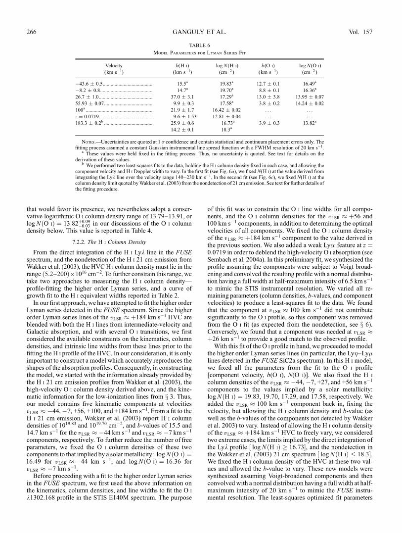
TABLE 6

Model Parameters for Lyman Series Fit

Velocity

(km s�1)

b(H i)

(km s�1)

logN (H i)

(cm�2 )

b(O i)

(km s�1)

logN (O i)

(cm�2 )

�43.6 � 0.5...................................... 15.5a 19.83a 12.7 � 0.1 16.49a

�8.2 � 0.8........................................ 14.7a 19.70a 8.8 � 0.1 16.36a

26.7 � 1.0......................................... 37.0 � 3.1 17.29a 13.0 � 3.8 13.95 � 0.07

55.93 � 0.07..................................... 9.9 � 0.3 17.58a 3.8 � 0.2 14.24 � 0.02

100a ................................................... 21.9 � 1.7 16.42 � 0.02 . . . . . .

z ¼ 0:0719......................................... 9.6 � 1.53 12.81 � 0.04 . . . . . .183.3 � 0.2b ..................................... 25.9 � 0.6 16.73a 3.9 � 0.3 13.82a

14.2 � 0.1 18.3a

Notes.—Uncertainties are quoted at 1 � confidence and contain statistical and continuum placement errors only. Thefitting process assumed a constant Gaussian instrumental line spread function with a FWHM resolution of 20 km s�1.

a These values were held fixed in the fitting process. Thus, no uncertainty is quoted. See text for details on thederivation of these values.

b We performed two least-squares fits to the data, holding the H i column density fixed in each case, and allowing thecomponent velocity and H i Doppler width to vary. In the first fit (see Fig. 6a), we fixed N(H i) at the value derived fromintegrating the Lyk line over the velocity range 140–230 km s�1. In the second fit (see Fig. 6c), we fixed N(H i) at thecolumn density limit quoted byWakker et al. (2003) from the nondetection of 21 cm emission. See text for further details ofthe fitting procedure.


are listed in Table 6 (along with the corresponding O i param-eters from the preliminary fit). In Figure 6 (panels a and c), weshow the best-fit models for the two extreme cases, along withthe same model without the contribution of the HVC, for thehigher order Lyman series. In addition, we show the contributionof the O i absorption. The differences in the two extreme casesare minor, with the most significant change arising in the Lytransition. Neither model can be clearly ruled out at the 2 � level.We therefore consider this full range a 95% confidence intervalfor the H i column density.

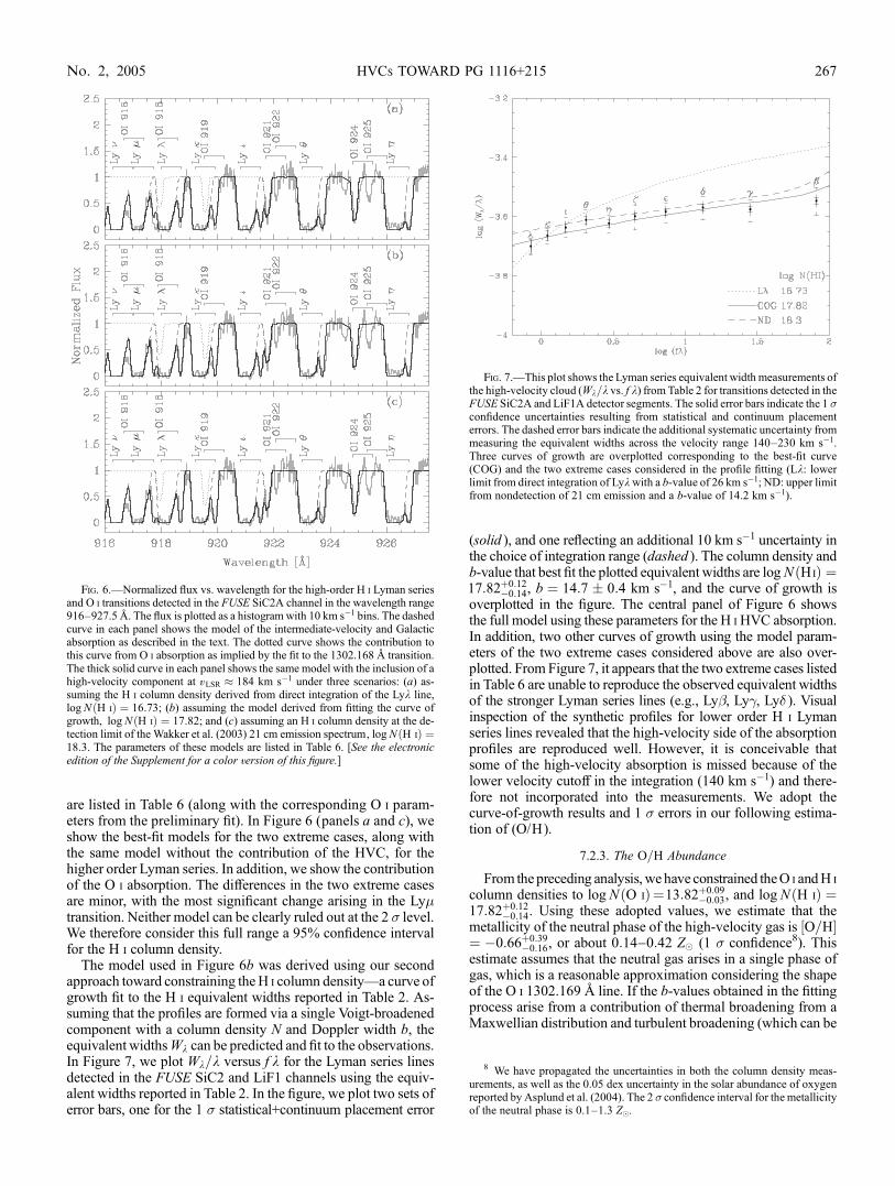
The model used in Figure 6b was derived using our secondapproach toward constraining theH i column density—a curve ofgrowth fit to the H i equivalent widths reported in Table 2. As-suming that the profiles are formed via a single Voigt-broadenedcomponent with a column density N and Doppler width b, theequivalent widthsWk can be predicted and fit to the observations.In Figure 7, we plot Wk=k versus f k for the Lyman series linesdetected in the FUSE SiC2 and LiF1 channels using the equiv-alent widths reported in Table 2. In the figure, we plot two sets oferror bars, one for the 1 � statistical+continuum placement error

(solid ), and one reflecting an additional 10 km s�1 uncertainty inthe choice of integration range (dashed ). The column density andb-value that best fit the plotted equivalent widths are log NðH iÞ ¼17:82þ0:12

�0:14, b ¼ 14:7 � 0:4 km s�1, and the curve of growth isoverplotted in the figure. The central panel of Figure 6 showsthe full model using these parameters for the H iHVC absorption.In addition, two other curves of growth using the model param-eters of the two extreme cases considered above are also over-plotted. From Figure 7, it appears that the two extreme cases listedin Table 6 are unable to reproduce the observed equivalent widthsof the stronger Lyman series lines (e.g., Ly�, Ly, Ly� ). Visualinspection of the synthetic profiles for lower order H i Lymanseries lines revealed that the high-velocity side of the absorptionprofiles are reproduced well. However, it is conceivable thatsome of the high-velocity absorption is missed because of thelower velocity cutoff in the integration (140 km s�1) and there-fore not incorporated into the measurements. We adopt thecurve-of-growth results and 1 � errors in our following estima-tion of (O/H).

7.2.3. The O=H Abundance

From the preceding analysis, we have constrained theO i andH i

column densities to log NðO iÞ ¼13:82þ0:09�0:03, and log NðH iÞ ¼

17:82þ0:12�0:14. Using these adopted values, we estimate that the

metallicity of the neutral phase of the high-velocity gas is ½O=H�¼ �0:66þ0:39

�0:16, or about 0:14 0:42 Z (1 � confidence8). Thisestimate assumes that the neutral gas arises in a single phase ofgas, which is a reasonable approximation considering the shapeof the O i 1302.169 8 line. If the b-values obtained in the fittingprocess arise from a contribution of thermal broadening from aMaxwellian distribution and turbulent broadening (which can be

Fig. 6.—Normalized flux vs. wavelength for the high-order H i Lyman seriesand O i transitions detected in the FUSE SiC2A channel in the wavelength range916–927.58. The flux is plotted as a histogram with 10 km s�1 bins. The dashedcurve in each panel shows the model of the intermediate-velocity and Galacticabsorption as described in the text. The dotted curve shows the contribution tothis curve from O i absorption as implied by the fit to the 1302.168 8 transition.The thick solid curve in each panel shows the same model with the inclusion of ahigh-velocity component at vLSR � 184 km s�1 under three scenarios: (a) as-suming the H i column density derived from direct integration of the Lyk line,logNðH iÞ ¼ 16:73; (b) assuming the model derived from fitting the curve ofgrowth, logNðH iÞ ¼ 17:82; and (c) assuming an H i column density at the de-tection limit of the Wakker et al. (2003) 21 cm emission spectrum, logNðH iÞ ¼18:3. The parameters of these models are listed in Table 6. [See the electronicedition of the Supplement for a color version of this figure.]

Fig. 7.—This plot shows the Lyman series equivalent width measurements ofthe high-velocity cloud (Wk=k vs. f k) from Table 2 for transitions detected in theFUSE SiC2A and LiF1A detector segments. The solid error bars indicate the 1 �confidence uncertainties resulting from statistical and continuum placementerrors. The dashed error bars indicate the additional systematic uncertainty frommeasuring the equivalent widths across the velocity range 140–230 km s�1.Three curves of growth are overplotted corresponding to the best-fit curve(COG) and the two extreme cases considered in the profile fitting (Lk: lowerlimit from direct integration of Lykwith a b-value of 26 km s�1; ND: upper limitfrom nondetection of 21 cm emission and a b-value of 14.2 km s�1).

8 We have propagated the uncertainties in both the column density meas-urements, as well as the 0.05 dex uncertainty in the solar abundance of oxygenreported by Asplund et al. (2004). The 2 � confidence interval for the metallicityof the neutral phase is 0.1–1.3 Z.

HVCs TOWARD PG 1116+215 267No. 2, 2005

characterized by a Gaussian of width bturb), we can constrain theseparate contributions of these broadening mechanisms: b2 ¼ð2kT=mÞ þ b2turb, where k is the Boltzmann constant andm is themass of the atom. From the inferred b-values of O i and H i, weplace the following constraints on the two values: T ¼ 11;400 �800 K, and bturb ¼ 1:9 � 0:7 km s�1. These quantities should beconsidered rough gauges of the temperature and turbulence inthe neutral gas since the absorptionmay contain substructure thatis blended in velocity.

In addition to the metallicity, we can consider the abundancesof other elements relative to oxygen in the neutral phase of thehigh-velocity gas. Of the ions with transitions observed, thefollowing are expected to dominate in a neutral phase: C ii, N i,O i, Mg ii, Si ii, P ii, S ii, Fe ii. (Most of these are singly ionizedstages, for which the ionization potential for creation is below13.6 eV.) If the relative abundances in this neutral phase followeda solar pattern (Table 7) with no ionization corrections the pre-dicted elemental column densities implied by the O i columndensity ½NðXÞ ¼ NðO iÞðX=OÞ� would be log NðCÞ ¼ 13:75,log NðNÞ ¼ 13:09,log NðMgÞ ¼ logNðSiÞ ¼ 12:70,logNðPÞ ¼10:73, log NðSÞ ¼ 12:43, and log NðFeÞ ¼ 12:61. Comparisonof these scaled column densities with the column densities re-ported in Table 4 reveals that the column density for every de-tected singly ionized species listed above exceeds the expectedcolumn density for neutral gas. (The column density upper limitson neutral and other singly ionized species covered by our dataset are not sufficiently restrictive to place useful constraints onrelative abundances.) There are only two possible scenarios thatcan explain this: (1) the relative elemental abundances deviatefrom the solar pattern, or (2) ionized gas contributes significantlyto the observed column densities. While the former scenariomight explain the relative abundance of iron to oxygen with theinvocation of different enrichment scenarios, it is unlikely toexplain the relative abundances of oxygen, magnesium, andsilicon, which are all� -process elements.We conclude that thereare significant ionization corrections for this low-ionization ma-terial that must be considered in order to constrain the relativeelemental abundances of the HVC. To first order, we can roughlyestimate the magnitude of this ionization correction by consid-ering the Si ii column density, since the apparent column densityprofile of Si ii appears to trace that of O i (see Fig. 5). Using thepredicted and observed column densities for Si ii, we estimatethat ionized gas contributesk90% (3 � confidence) of the ob-served column density. This implies a substantial ionizationcorrection is needed to transform Si ii to a total silicon abundancein the cloud. The correction could, in fact, be larger if the HVCcontains dust, since the ionization correction only accounts for

the gas phase atoms. In the next section, we examine variousscenarios to explain the ionization of this gas.

7.3. Ionization

As we have pointed out in the previous sections, in order toinfer relative abundances of metals and address, for example,the possible presence of dust, it is imperative to consider theeffects of ionization on the observed column density ratios.Understanding the ionization is important as such an analysisyields information on the structure of the gas, the mass con-tained in the neutral and ionized gas, and constraints on thepossible locations of the gas.In the previous section, we estimated the approximate contri-

bution of the neutral phase (where O i is produced) to the ob-served column densities of low-ionization species, motivatingthe need for an additional low-ionization phase. We can apply asimilar first order comparison of the amount of high-ionizationgas producing the O vi to the neutral gas producing the O i. Therelative amounts of gas in each phase can be estimated thoughthe column densities of O vi and O i corrected for their relativeionization fractions ( f ), and abundances [(O/H)]:

NðHÞHIGNðHÞNG

¼ NðO viÞ f �1O vi

ðO=HÞ�1HIG

NðO iÞ f �1O i

ðO=HÞ�1NG

; ð4Þ

where the subscripts HIG and NG denote high-ionization gasand neutral gas, respectively. We assume that the oxygenabundances of the two phases are similar ½ðO=HÞHIG �ðO=HÞNG� and that all the oxygen in the neutral gas is in the formof O i ( fO i � 1). The ionization fraction of O vi rarely exceeds20% (Sembach et al. 2003; Tripp & Savage 2000), so we canplace a lower limit on amount of gas in the high-ionizationphase relative to the neutral phase: NðHÞHIG=NðHÞNG k0:2�1 ;1014:00=1013:82 ¼ 7:6.

For a more detailed understanding of the ionization of thehigh-velocity gas, we consider the kinematics of the HVC tomotivate the scenario under which the gas is ionized. The ap-parent column density profiles shown in Figure 5, which areordered in ionization potential of the depicted species, providea starting point. The complex kinematics of the profiles easilyrule out absorption originating in a medium having a singledensity and temperature. It is physically impossible to explain,for example, the drastically different kinematics of O i and O vi

in such a phase. However, the velocity alignments of the pro-files suggest a common origin. This rules out scenarios such aspure photoionization by the extragalactic background in a low-density plasma (e.g., Nicastro et al. 2002). Furthermore, var-iants of this type of scenario also have difficulty explaining boththe ionization of the HVC and the kinematical properties of thehigh-velocity absorption lines.We propose that the kinematics and ionization of the high-

velocity gas are qualitatively consistent with a diffuse cloud thatis moving away from the Galactic disk and is being stripped by ahot, low-density external medium such as the Galactic halo orcorona. A schematic depiction of the cloud structure is shown inFigure 8. The neutral gas resides in the core of the cloud, withsome low-ionization gas surrounding it. A leading ‘‘shock’’ mayexist depending on the density contrast between the cloud andexternal medium. [It is unlikely to be a classical shock as thevelocity of cloud is of the same order as the sound speed of a hot(>106 K), low-density (P10�4 cm�3) external medium.] As thestripped matter equilibrates with the external medium, it will heat

TABLE 7

Adopted Solar Abundances

Element Aa Reference

C............................................. 8.39 Allende Prieto et al. (2002)

N............................................. 7.931 Holweger (2001)

O............................................. 8.66 Asplund et al. (2004)

Mg.......................................... 7.538 Holweger (2001)

Al............................................ 6.48 Anders & Grevesse (1989)

Si ............................................ 7.536 Holweger (2001)

P ............................................. 5.57 Anders & Grevesse (1989)

S ............................................. 7.27 Anders & Grevesse (1989)

Fe............................................ 7.448 Holweger (2001)

a We adopt the standard notation for abundances: AðXÞ ¼ 12 þlog ½NðXÞ=NðHÞ�.


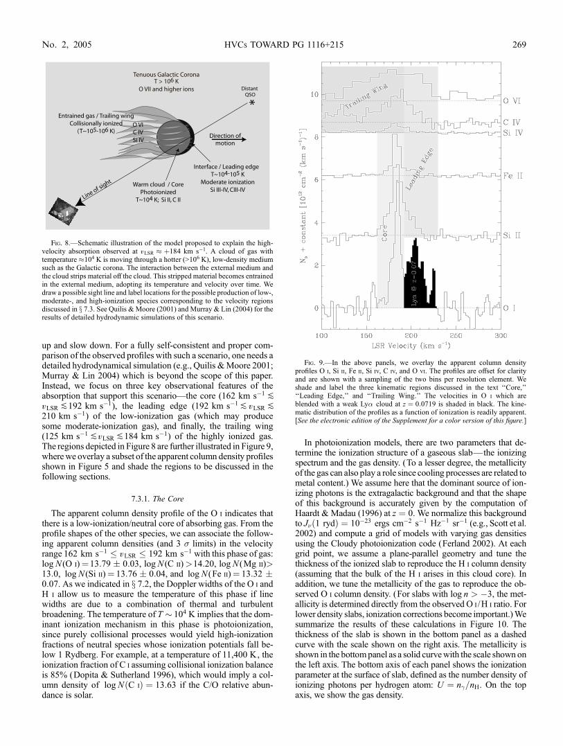
up and slow down. For a fully self-consistent and proper com-parison of the observed profiles with such a scenario, one needs adetailed hydrodynamical simulation (e.g., Quilis &Moore 2001;Murray & Lin 2004) which is beyond the scope of this paper.Instead, we focus on three key observational features of theabsorption that support this scenario—the core (162 km s�1 PvLSR P192 km s�1), the leading edge (192 km s�1P vLSR P210 km s�1) of the low-ionization gas (which may producesome moderate-ionization gas), and finally, the trailing wing(125 km s�1 PvLSR P184 km s�1) of the highly ionized gas.The regions depicted in Figure 8 are further illustrated in Figure 9,wherewe overlay a subset of the apparent column density profilesshown in Figure 5 and shade the regions to be discussed in thefollowing sections.

7.3.1. The Core

The apparent column density profile of the O i indicates thatthere is a low-ionization/neutral core of absorbing gas. From theprofile shapes of the other species, we can associate the follow-ing apparent column densities (and 3 � limits) in the velocityrange 162 km s�1 � vLSR � 192 km s�1 with this phase of gas:log N (O i)¼13:79 � 0:03, logN (C ii)>14:20, logN (Mg ii)>13:0, log N (Si ii)¼ 13:76 � 0:04, and log N (Fe ii)¼ 13:32 �0:07. As we indicated in x 7.2, the Doppler widths of the O i andH i allow us to measure the temperature of this phase if linewidths are due to a combination of thermal and turbulentbroadening. The temperature of T � 104 K implies that the dom-inant ionization mechanism in this phase is photoionization,since purely collisional processes would yield high-ionizationfractions of neutral species whose ionization potentials fall be-low 1 Rydberg. For example, at a temperature of 11,400 K, theionization fraction of C i assuming collisional ionization balanceis 85% (Dopita & Sutherland 1996), which would imply a col-umn density of log NðC iÞ ¼ 13:63 if the C/O relative abun-dance is solar.

In photoionization models, there are two parameters that de-termine the ionization structure of a gaseous slab—the ionizingspectrum and the gas density. (To a lesser degree, the metallicityof the gas can also play a role since cooling processes are related tometal content.) We assume here that the dominant source of ion-izing photons is the extragalactic background and that the shapeof this background is accurately given by the computation ofHaardt & Madau (1996) at z ¼ 0. We normalize this backgroundto J�ð1 rydÞ ¼ 10�23 ergs cm�2 s�1 Hz�1 sr�1 (e.g., Scott et al.2002) and compute a grid of models with varying gas densitiesusing the Cloudy photoionization code (Ferland 2002). At eachgrid point, we assume a plane-parallel geometry and tune thethickness of the ionized slab to reproduce the H i column density(assuming that the bulk of the H i arises in this cloud core). Inaddition, we tune the metallicity of the gas to reproduce the ob-served O i column density. (For slabs with log n > �3, the met-allicity is determined directly from the observed O i /H i ratio. Forlower density slabs, ionization corrections become important.)Wesummarize the results of these calculations in Figure 10. Thethickness of the slab is shown in the bottom panel as a dashedcurve with the scale shown on the right axis. The metallicity isshown in the bottompanel as a solid curvewith the scale shown onthe left axis. The bottom axis of each panel shows the ionizationparameter at the surface of slab, defined as the number density ofionizing photons per hydrogen atom: U ¼ n=nH. On the topaxis, we show the gas density.

Fig. 8.—Schematic illustration of the model proposed to explain the high-velocity absorption observed at vLSR � þ184 km s�1. A cloud of gas withtemperature �104 K is moving through a hotter (>106 K), low-density mediumsuch as the Galactic corona. The interaction between the external medium andthe cloud strips material off the cloud. This stripped material becomes entrainedin the external medium, adopting its temperature and velocity over time. Wedraw a possible sight line and label locations for the possible production of low-,moderate-, and high-ionization species corresponding to the velocity regionsdiscussed in x 7.3. See Quilis & Moore (2001) and Murray & Lin (2004) for theresults of detailed hydrodynamic simulations of this scenario.

Fig. 9.—In the above panels, we overlay the apparent column densityprofiles O i, Si ii, Fe ii, Si iv, C iv, and O vi. The profiles are offset for clarityand are shown with a sampling of the two bins per resolution element. Weshade and label the three kinematic regions discussed in the text ‘‘Core,’’‘‘Leading Edge,’’ and ‘‘Trailing Wing.’’ The velocities in O i which areblended with a weak Ly� cloud at z ¼ 0:0719 is shaded in black. The kine-matic distribution of the profiles as a function of ionization is readily apparent.[See the electronic edition of the Supplement for a color version of this figure.]

HVCs TOWARD PG 1116+215 269No. 2, 2005

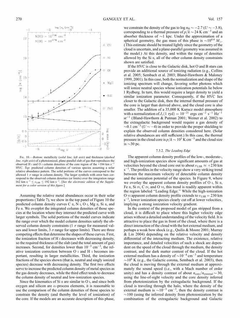
Assuming the relative metal abundances occur in their solarproportions (Table 7), we show in the top panel of Figure 10 thepredicted column density curves C ii, N i, O i, Mg ii, Si ii, andFe ii. We overplot the integrated column densities of those spe-cies at the location where they intersect the predicted curve withlarger symbols. The solid portions of the model curves indicatethe range over which the model column densities satisfy the ob-served column density constraints (1 � range for measured val-ues and lower limits, 3 � range for upper limits). There are threecompeting effects that determine the shapes of these curves. First,the ionization fraction of H i decreases with decreasing density,so the required thickness of the slab (and the total amount of gas)increases. Second, for densities lower than 10�3 cm�3, the rel-ative ionization correction between O i and H i becomes im-portant, resulting in larger metallicities. Third, the ionizationfractions of the species shown (that is, neutral and singly ionizedspecies) decrease with decreasing density. The first two effectsserve to increase the predicted column density of metal species asthe gas density decreases, while the third effect tends to decreasethe column density of neutral and low-ionization species.

Since the kinematics of Si ii are similar to O i, and since bothoxygen and silicon are � -process elements, it is reasonable touse the comparison of the column densities of those species toconstrain the density (and thereby the level of ionization) ofthe core. If the models are an accurate description of this phase,

we constrain the density of the gas to log nH ��2:7 (U ��3:8),corresponding to a thermal pressure of p=k � 24 K cm�3 and anabsorber thickness of �1 kpc. Under the approximation of aspherical geometry, the gas mass of this phase is �104.4 M.(This estimate should be treated lightly since the geometry of thecloud is uncertain, and a plane-parallel geometry was assumed inthe model.) At this density, and within the range of densitiesallowed by the Si ii, all of the other column density constraintsshown are satisfied.If the HVC is close to the Galactic disk, hot O and B stars can

provide an additional source of ionizing radiation (e.g., Collinset al. 2005; Sembach et al. 2003; Bland-Hawthorn & Maloney1999, 2001). In this case, both the normalization and shape of theionizing spectrum will change, favoring softer photons whichwill ionize neutral species whose ionization potentials lie below1 Rydberg. In turn, this would require a larger density to yield asimilar ionization parameter. Consequently, if the HVC liescloser to the Galactic disk, then the internal thermal pressure ofthe core is larger than derived above, and the cloud core is alsosmaller. The addition of a 35,000 K Kurucz model atmospherewith a normalization of J�ð1 rydÞ ¼ 10�21 ergs cm�2 s�1 Hz�1

sr�1 (Bland-Hawthorn & Putman 2001; Weiner et al. 2002) tothe extragalactic background would require a gas density of�0.1 cm�3 (U ��4) in order to provide the proper shielding toexplain the observed column densities considered here. (Solarrelative abundances are still sufficient.) In this case, the thermalpressure in the cloud core is p=k � 103 K cm�3 and the cloud sizeis �30 pc.

7.3.2. The LeadinggEdgge

The apparent column density profiles of the low-, moderate-,and high-ionization species show significant amounts of gas atvelocities beyond the cloud core out to about vLSR � þ230 kms�1. The profiles in the velocity range show a very striking trendbetween the maximum velocity of detectable column densityand the ionization potential of the species. In Figure 9, wherewe overlay the apparent column density profiles of O i, Si ii,Fe ii, Si iv, C iv, and O vi, this trend is readily apparent withinthe region labeled ‘‘Leading Edge.’’ While the high-ionizationO vi apparent column density profile extends to vLSR¼ 230 kms�1, lower ionization species clearly cut off at lower velocities ,implying a strong ionization velocity gradient.In the context of the proposed model of gas stripped from a

cloud, it is difficult to place where this higher velocity edgearises without a detailed understanding of the velocity field. It isattractive to place the gas in front of the cloud, where there is adirect interaction of the cloud with the hot external medium, andperhaps a weak bow shock (e.g., Quilis & Moore 2001; Murray& Lin 2004) depending on the relative velocity and densitydifferential of the interacting medium. The existence, relativeimportance, and detailed velocities of such a shock are depen-dent on the speed of the cloud through the medium, the densitycontrast, and the dark matter content of the cloud. If the hotexternal medium has a density of�10�4 cm�3 and temperature�106 K (e.g., the Galactic corona, Sembach et al. 2003), thenthe cloud is moving through the external medium at approxi-mately the sound speed (i.e., with a Mach number of orderunity) and has a density contrast of about ncore=nexternal � 30,using the line-of-sight velocity and the core density inferredfrom photoionization by the extragalactic background. If thecloud is traveling through the halo, where the density of theexternal medium is �10�3 cm�3, then the density contrast is�100 (using the inferred density from photoionization by thecombination of the extragalactic background and Galactic

Fig. 10.—Bottom: metallicity (solid line, left axis) and thickness (dashedline, right axis) of a photoionized, plane-parallel slab of gas that reproduces theobserved H i and O i column densities of the core region of the +184 km s�1

HVC. Top: predicted column densities of various species assuming a solarrelative abundance pattern. The solid portions of the curves correspond to theallowed 1 � range in column density. The larger symbols with error bars cor-respond to the observed column densities (or limits) over the integration range162 km s�1 � vLSR � 192 km s�1. [See the electronic edition of the Supple-ment for a color version of this figure.]


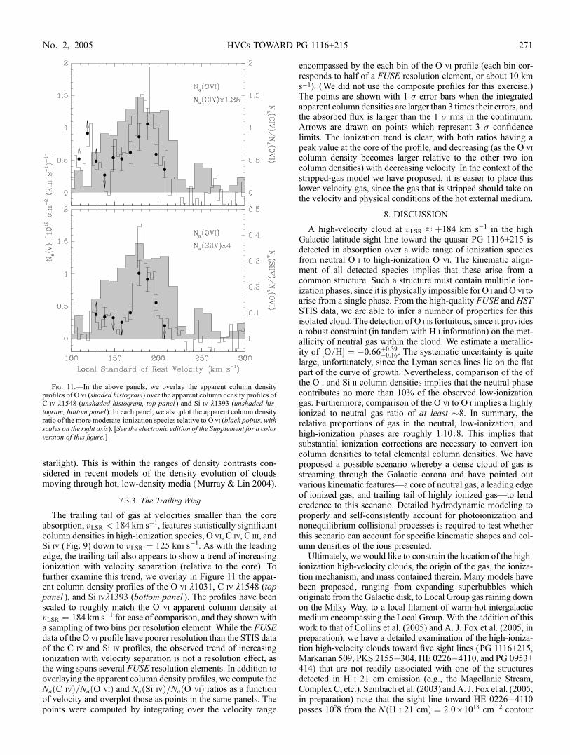
starlight). This is within the ranges of density contrasts con-sidered in recent models of the density evolution of cloudsmoving through hot, low-density media (Murray & Lin 2004).

7.3.3. The TrailinggWingg

The trailing tail of gas at velocities smaller than the coreabsorption, vLSR < 184 km s�1, features statistically significantcolumn densities in high-ionization species, O vi, C iv, C iii, andSi iv (Fig. 9) down to vLSR ¼ 125 km s�1. As with the leadingedge, the trailing tail also appears to show a trend of increasingionization with velocity separation (relative to the core). Tofurther examine this trend, we overlay in Figure 11 the appar-ent column density profiles of the O vi k1031, C iv k1548 (toppanel ), and Si ivk1393 (bottom panel ). The profiles have beenscaled to roughly match the O vi apparent column density atvLSR ¼ 184 km s�1 for ease of comparison, and they shown witha sampling of two bins per resolution element. While the FUSEdata of the O vi profile have poorer resolution than the STIS dataof the C iv and Si iv profiles, the observed trend of increasingionization with velocity separation is not a resolution effect, asthe wing spans several FUSE resolution elements. In addition tooverlaying the apparent column density profiles, we compute theNaðC ivÞ=NaðO viÞ and NaðSi ivÞ=NaðO viÞ ratios as a functionof velocity and overplot those as points in the same panels. Thepoints were computed by integrating over the velocity range

encompassed by the each bin of the O vi profile (each bin cor-responds to half of a FUSE resolution element, or about 10 kms�1). (We did not use the composite profiles for this exercise.)The points are shown with 1 � error bars when the integratedapparent column densities are larger than 3 times their errors, andthe absorbed flux is larger than the 1 � rms in the continuum.Arrows are drawn on points which represent 3 � confidencelimits. The ionization trend is clear, with both ratios having apeak value at the core of the profile, and decreasing (as the O vi

column density becomes larger relative to the other two ioncolumn densities) with decreasing velocity. In the context of thestripped-gas model we have proposed, it is easier to place thislower velocity gas, since the gas that is stripped should take onthe velocity and physical conditions of the hot external medium.

8. DISCUSSION

A high-velocity cloud at vLSR � þ184 km s�1 in the highGalactic latitude sight line toward the quasar PG 1116+215 isdetected in absorption over a wide range of ionization speciesfrom neutral O i to high-ionization O vi. The kinematic align-ment of all detected species implies that these arise from acommon structure. Such a structure must contain multiple ion-ization phases, since it is physically impossible for O i andO vi toarise from a single phase. From the high-quality FUSE and HSTSTIS data, we are able to infer a number of properties for thisisolated cloud. The detection of O i is fortuitous, since it providesa robust constraint (in tandem with H i information) on the met-allicity of neutral gas within the cloud. We estimate a metallic-ity of ½O=H� ¼ �0:66þ0:39

�0:16. The systematic uncertainty is quitelarge, unfortunately, since the Lyman series lines lie on the flatpart of the curve of growth. Nevertheless, comparison of the ofthe O i and Si ii column densities implies that the neutral phasecontributes no more than 10% of the observed low-ionizationgas. Furthermore, comparison of the O vi to O i implies a highlyionized to neutral gas ratio of at least �8. In summary, therelative proportions of gas in the neutral, low-ionization, andhigh-ionization phases are roughly 1:10 :8. This implies thatsubstantial ionization corrections are necessary to convert ioncolumn densities to total elemental column densities. We haveproposed a possible scenario whereby a dense cloud of gas isstreaming through the Galactic corona and have pointed outvarious kinematic features—a core of neutral gas, a leading edgeof ionized gas, and trailing tail of highly ionized gas—to lendcredence to this scenario. Detailed hydrodynamic modeling toproperly and self-consistently account for photoionization andnonequilibrium collisional processes is required to test whetherthis scenario can account for specific kinematic shapes and col-umn densities of the ions presented.

Ultimately, we would like to constrain the location of the high-ionization high-velocity clouds, the origin of the gas, the ioniza-tion mechanism, and mass contained therein. Many models havebeen proposed, ranging from expanding superbubbles whichoriginate from the Galactic disk, to Local Group gas raining downon the Milky Way, to a local filament of warm-hot intergalacticmedium encompassing the Local Group.With the addition of thiswork to that of Collins et al. (2005) and A. J. Fox et al. (2005, inpreparation), we have a detailed examination of the high-ioniza-tion high-velocity clouds toward five sight lines (PG 1116+215,Markarian 509, PKS 2155�304, HE 0226�4110, and PG 0953+414) that are not readily associated with one of the structuresdetected in H i 21 cm emission (e.g., the Magellanic Stream,Complex C, etc.). Sembach et al. (2003) andA. J. Fox et al. (2005,in preparation) note that the sight line toward HE 0226�4110passes 10N8 from the NðH i 21 cmÞ ¼ 2:0 ; 1018 cm�2 contour

Fig. 11.—In the above panels, we overlay the apparent column densityprofiles of O vi (shaded histogram) over the apparent column density profiles ofC iv k1548 (unshaded histogram, top panel ) and Si iv k1393 (unshaded his-togram, bottom panel ). In each panel, we also plot the apparent column densityratio of the more moderate-ionization species relative to O vi (black points, withscales on the right axis). [See the electronic edition of the Supplement for a colorversion of this figure.]

HVCs TOWARD PG 1116+215 271No. 2, 2005

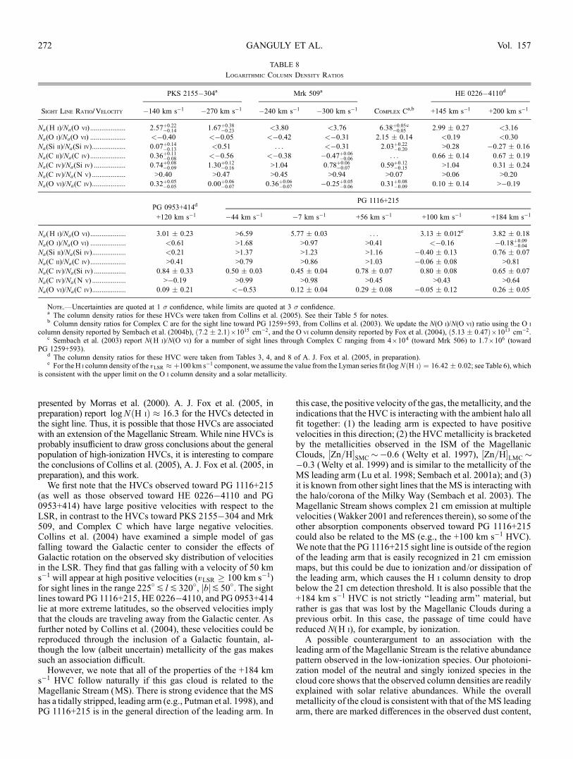
presented by Morras et al. (2000). A. J. Fox et al. (2005, inpreparation) report log NðH iÞ � 16:3 for the HVCs detected inthe sight line. Thus, it is possible that those HVCs are associatedwith an extension of the Magellanic Stream. While nine HVCs isprobably insufficient to draw gross conclusions about the generalpopulation of high-ionization HVCs, it is interesting to comparethe conclusions of Collins et al. (2005), A. J. Fox et al. (2005, inpreparation), and this work.

We first note that the HVCs observed toward PG 1116+215(as well as those observed toward HE 0226�4110 and PG0953+414) have large positive velocities with respect to theLSR, in contrast to the HVCs toward PKS 2155�304 and Mrk509, and Complex C which have large negative velocities.Collins et al. (2004) have examined a simple model of gasfalling toward the Galactic center to consider the effects ofGalactic rotation on the observed sky distribution of velocitiesin the LSR. They find that gas falling with a velocity of 50 kms�1 will appear at high positive velocities (vLSR � 100 km s�1)for sight lines in the range 225�P lP 320�, jbjP50�. The sightlines toward PG 1116+215, HE 0226�4110, and PG 0953+414lie at more extreme latitudes, so the observed velocities implythat the clouds are traveling away from the Galactic center. Asfurther noted by Collins et al. (2004), these velocities could bereproduced through the inclusion of a Galactic fountain, al-though the low (albeit uncertain) metallicity of the gas makessuch an association difficult.

However, we note that all of the properties of the +184 kms�1 HVC follow naturally if this gas cloud is related to theMagellanic Stream (MS). There is strong evidence that the MShas a tidally stripped, leading arm (e.g., Putman et al. 1998), andPG 1116+215 is in the general direction of the leading arm. In

this case, the positive velocity of the gas, the metallicity, and theindications that the HVC is interacting with the ambient halo allfit together: (1) the leading arm is expected to have positivevelocities in this direction; (2) the HVCmetallicity is bracketedby the metallicities observed in the ISM of the MagellanicClouds, ½Zn=H�SMC ��0:6 (Welty et al. 1997), ½Zn=H�LMC ��0:3 (Welty et al. 1999) and is similar to the metallicity of theMS leading arm (Lu et al. 1998; Sembach et al. 2001a); and (3)it is known from other sight lines that the MS is interacting withthe halo/corona of the Milky Way (Sembach et al. 2003). TheMagellanic Stream shows complex 21 cm emission at multiplevelocities (Wakker 2001 and references therein), so some of theother absorption components observed toward PG 1116+215could also be related to the MS (e.g., the +100 km s�1 HVC).We note that the PG 1116+215 sight line is outside of the regionof the leading arm that is easily recognized in 21 cm emissionmaps, but this could be due to ionization and/or dissipation ofthe leading arm, which causes the H i column density to dropbelow the 21 cm detection threshold. It is also possible that the+184 km s�1 HVC is not strictly ‘‘leading arm’’ material, butrather is gas that was lost by the Magellanic Clouds during aprevious orbit. In this case, the passage of time could havereduced N(H i), for example, by ionization.A possible counterargument to an association with the

leading arm of the Magellanic Stream is the relative abundancepattern observed in the low-ionization species. Our photoioni-zation model of the neutral and singly ionized species in thecloud core shows that the observed column densities are readilyexplained with solar relative abundances. While the overallmetallicity of the cloud is consistent with that of the MS leadingarm, there are marked differences in the observed dust content,

TABLE 8

Logarithmic Column Density Ratios

PKS 2155�304a Mrk 509a HE 0226�4110d

Sight Line Ratio/Velocity �140 km s�1 �270 km s�1 �240 km s�1 �300 km s�1Complex Ca,b +145 km s�1 +200 km s�1

PG 0953+

+120 km

Na(H i)/Na(O vi) ................... 2:57þ0:22�0:14 1:67þ0:38

�0:23 <3.80 <3.76 6:38þ0:05�0:05

c 2.99 � 0.27 <3.16 3.01 �Na(O i)/Na(O vi) ................... <�0.40 <�0.05 <�0.42 <�0.31 2.15 � 0.14 <0.19 <0.30 <0.6

Na(Si ii)/Na(Si iv).................. 0:07þ0:14�0:13 <0.51 . . . <�0.31 2:03þ0:22

�0:20 >0.28 �0.27 � 0.16 <0.2

Na(C ii)/Na(C iv) ................... 0:36þ0:11�0:08 <�0.56 <�0.38 �0:47þ0:06

�0:06 . . . 0.66 � 0.14 0.67 � 0.19 >0.4

Na(C iv)/Na(Si iv) ................. 0:74þ0:08�0:09 1:30þ0:12

�0:16 >1.04 0:78þ0:06�0:07 0:59þ0:12

�0:15 >1.04 0.31 � 0.24 0.84 �Na(C iv)/Na(N v) .................. >0.40 >0.47 >0.45 >0.94 >0.07 >0.06 >0.20 >�0.

Na(O vi)/Na(C iv).................. 0:32þ0:05�0:05 0:00þ0:06

�0:07 0:36þ0:06�0:07 �0:25þ0:05

�0:06 0:31þ0:08�0:09 0.10 � 0.14 >�0.19 0.09 �

PG 1116+215PG 0953+414d

+120 km s�1 �44 km s�1 �7 km s�1 +56 km s�1 +100 km s�1 +184 km s�1

Na(H i)/Na(O vi) ................... 3.01 � 0.23 >6.59 5.77 � 0.03 . . . 3.13 � 0.012e 3.82 � 0.18

Na(O i)/Na(O vi) ................... <0.61 >1.68 >0.97 >0.41 <�0.16 �0:18þ0:09�0:04

Na(Si ii)/Na(Si iv).................. <0.21 >1.37 >1.23 >1.16 �0.40 � 0.13 0.76 � 0.07

Na(C ii)/Na(C iv) ................... >0.41 >0.79 >0.86 >1.03 �0.06 � 0.08 >0.81

Na(C iv)/Na(Si iv) ................. 0.84 � 0.33 0.50 � 0.03 0.45 � 0.04 0.78 � 0.07 0.80 � 0.08 0.65 � 0.07

Na(C iv)/Na(N v) .................. >�0.19 >0.99 >0.98 >0.45 >0.43 >0.64

Na(O vi)/Na(C iv).................. 0.09 � 0.21 <�0.53 0.12 � 0.04 0.29 � 0.08 �0.05 � 0.12 0.26 � 0.05

Note.—Uncertainties are quoted at 1 � confidence, while limits are quoted at 3 � confidence.a The column density ratios for these HVCs were taken from Collins et al. (2005). See their Table 5 for notes.b Column density ratios for Complex C are for the sight line toward PG 1259+593, from Collins et al. (2003). We update the N(O i)/N(O vi) ratio using the O i

column density reported by Sembach et al. (2004b), ð7:2 � 2:1Þ ; 1015 cm�2, and the O vi column density reported by Fox et al. (2004), ð5:13 � 0:47Þ ; 1013 cm�2.c Sembach et al. (2003) report N(H i)/N(O vi) for a number of sight lines through Complex C ranging from 4 ; 104 (toward Mrk 506) to 1:7 ; 106 (toward

PG 1259+593).d The column density ratios for these HVC were taken from Tables 3, 4, and 8 of A. J. Fox et al. (2005, in preparation).e For the H i column density of the vLSR � þ100 km s�1 component, we assume the value from the Lyman series fit (log NðH iÞ ¼ 16:42 � 0:02; see Table 6), which

is consistent with the upper limit on the O i column density and a solar metallicity.


and depletion patterns. Sembach et al. (2001a) report the de-tection of H2 in the MS leading arm in Lyman and Wernerabsorption against the spectrum of the bright Seyfert 1 galaxyNGC 3783 (l ¼ 287N5, b ¼ 23�). No molecular hydrogen isdetected in the PG 1116+215 +184 km s�1 HVC. In the MSleading arm, Si and Fe show signs of appreciable depletion by0.2 and 0.9 dex, respectively. Such a change to the relativeabundances of Si and Fe cannot explain the observed columndensities in the PG 1116+215 +184 km s�1 cloud core, if thephotoionization model is accurate. It is important to note,however, that the low-latitude sight line to NGC 3783 passesthrough a dense region of the leading arm where the contribu-tion of ionized gas to the observed column densities of singlyionized species is small (P10%–15%). The gas in the high-latitude PG 1116+215 +184 km s�1 cloud core, on the otherhand, is predominantly ionized andmore diffuse. Sembach et al.(2001a) estimate a density of nH ¼ 3:3 cm�3 for the H2 in thelow-latitude gas, which is at least 10 times larger than thedensity in the PG 1116+215 +184 km s�1 cloud core inferredfrom our photoionization model. In the PG 1116+215 +184 kms�1 HVC, we observe NðFe iiÞ=NðSi iiÞ ¼ 0:41, whereas in theMS leading arm toward NGC 3783, Sembach et al. (2001a)observed NðFe iiÞ=NðSi iiÞ ¼ 0:18. This difference is mostreadily explained by a combination of ionization and differingdegrees of heavy metal incorporation into dust grains. With theavailable data, it is not possible to unambiguously distinguishbetween these two effects, both of which modify N(Fe ii)/N(Si ii)in lower density environments where the ionization level istypically higher and the grain destruction is usually more com-plete than in denser, mainly neutral regions. Thus, it is stillpossible that the observed differences may be explained by thedestruction of dust grains, dissociation of molecules and ioni-zation as the MS leading arm gas continues to interact with thehotter external medium, particularly if the high-velocity gas to-ward PG 1116+215 (and perhaps PG 0953+414) is remnantstream material from an earlier (older) stream passage.

We can compare the gross characteristics of the highly ionizedHVCs by considering various column density ratios. In Table 8,we reproduce the column density ratios reported for the high-velocity clouds toward PKS 2155�304, and Mrk 509 (Collinset al. 2005, see their Table 5 for notes), and for Complex C asobserved along the PG 1259+593 sight line (Collins et al. 2003;Fox et al. 2004; Sembach et al. 2004a). We add three additionalhigh-velocity clouds from A. J. Fox et al. (2005, in preparation),and two high-velocity clouds from this work, as well as the threeGalactic ISM/IVC components observed along the PG 1116+215sight line. For comparison, we plot these ion ratios in Figure 12(see Table 9 for the ordering of clouds in the figure).

The column density ratios for the HVCs toward PG1116+215, HE 0226�4110, PG 0953+414, PKS 2155�304,and Mrk 509 tend to favor higher ionization gas, as evidencedby the O i /O vi constraints, in stark contrast to the low/inter-mediate-velocity clouds toward PG 1116+215 and Complex C.There is a clear distinction between Complex C (and the low/intermediate-velocity gas) and the high-ionization HVCs, withthe former being dominated by H i and the latter being domi-nated by H ii. This separation is also apparent in the Si ii/Si ivratio.

A possible argument against a Galactic origin for the highlyionized HVCs would be a comparison of the NðC ivÞ=NðSi ivÞcolumn density ratio. As reported by Sembach et al. (1997) in astudy of Radio Loops I and IV, this ratio remains fairly constantclose to and within the Galactic disk: log NðC ivÞ=NðSi ivÞ ¼0:58þ0:18

�0:30. Of the nine high-ionization HVCs, only three are

actually inconsistent with this range: the vLSR � þ145 km s�1

HVC toward HE 0226�4110, the vLSR � �270 km s�1 HVCtoward PKS 2155�304, and the vLSR � �240 km s�1 HVCtoward Mrk 509. Collins et al. (2005) note that the NðC ivÞ=NðSi ivÞ ratio for the HVCs toward PKS 2155�304 andMrk 509 is significantly higher than the ratio for gas within theGalactic disk or low halo, and they argue against a locationclose to or within the disk. The same ratio for the vLSR � þ184high-velocity cloud is not only consistent with the ratio reportedby Sembach et al. (1997) but is also consistent with the ratioreported by Collins et al. (2003) for Complex C. However, assummarized by Fox et al. (2004), there are several collisionalprocesses that can potentially explain the observed range of Civ/Si iv. Thus, for the majority of the highly ionized HVCs thathave been observed to date, we cannot rule out an origin near(or within) the Galactic disk based on the NðC ivÞ=NðSi ivÞcolumn density ratio.

Further comparison of the observed O vi /C iv column densityratios to the predicted ranges for the collisional processesconsidered by Fox et al. (2004) reveals that conductive inter-faces and shock ionization can account for observed ratios forboth the highly ionized HVCs (with one exception—vLSR ��300 km s�1 toward Mrk 509) and Complex C (see Table 5 fora summary of the model parameters and ranges considered).Thus, while the origins of HVCs may be varied (as indicated

Fig. 12.—This figure shows various column density ratios for the clouds inthe PG 1116+215 sight line (clouds 1–5), as well as the high-velocity cloudstoward HE 0226�4110 (clouds 6–7, A. J. Fox et al. 2005, in preparation), PG0953+414 (cloud 8, A. J. Fox et al. 2005, in preparation), PKS 2155�304(clouds 9–10, Collins et al. 2005), Mrk 509 (clouds 11–12, Collins et al. 2005),and Complex C (cloud 13, Collins et al. 2003; Fox et al. 2004; Sembach et al.2004a). See Table 9 for further information on the clouds. The shaded regionhighlights the column density ratios for the highly ionized HVCs studied indetail thus far. The dashed horizontal linemarks the ratio for the vLSR ¼ þ184 kms�1 HVC in the PG 1116+215 sight line (cloud 5).

HVCs TOWARD PG 1116+215 273No. 2, 2005

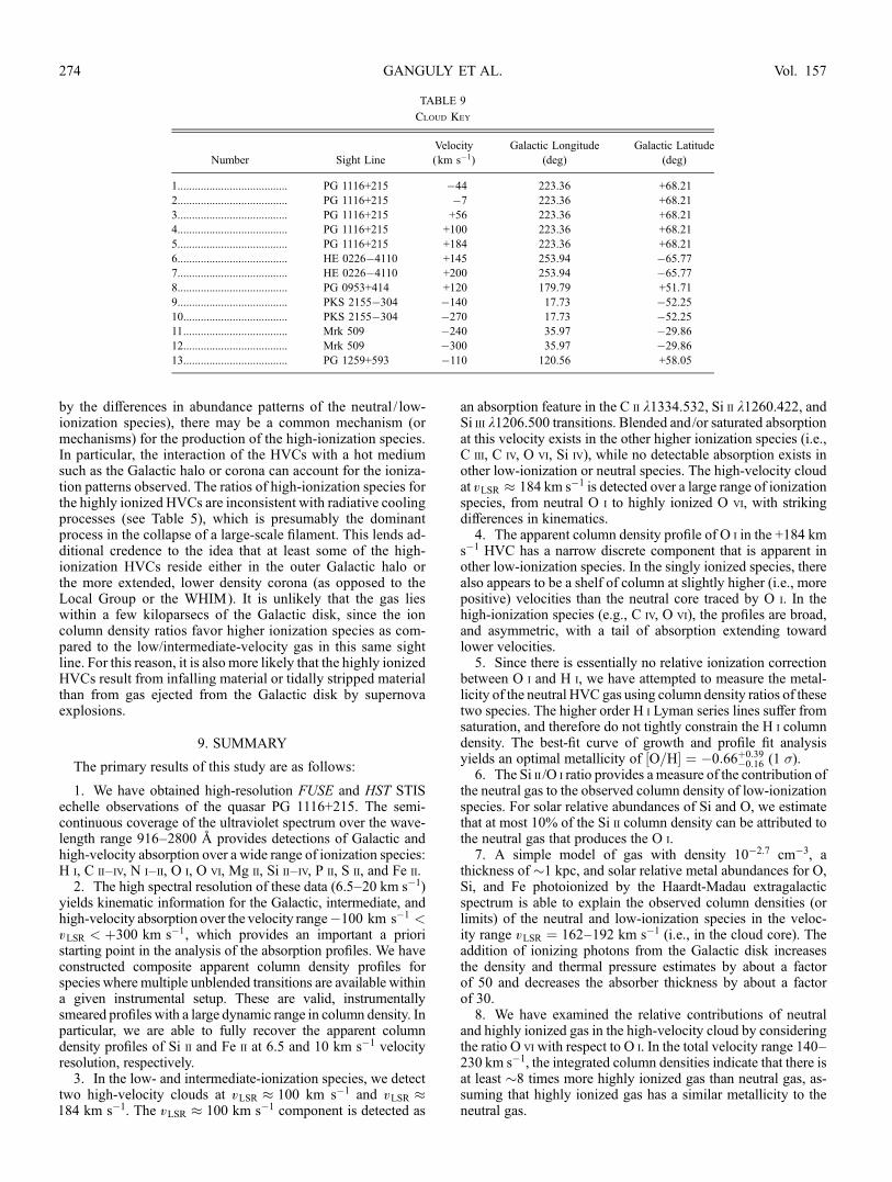
by the differences in abundance patterns of the neutral / low-ionization species), there may be a common mechanism (ormechanisms) for the production of the high-ionization species.In particular, the interaction of the HVCs with a hot mediumsuch as the Galactic halo or corona can account for the ioniza-tion patterns observed. The ratios of high-ionization species forthe highly ionized HVCs are inconsistent with radiative coolingprocesses (see Table 5), which is presumably the dominantprocess in the collapse of a large-scale filament. This lends ad-ditional credence to the idea that at least some of the high-ionization HVCs reside either in the outer Galactic halo orthe more extended, lower density corona (as opposed to theLocal Group or the WHIM). It is unlikely that the gas lieswithin a few kiloparsecs of the Galactic disk, since the ioncolumn density ratios favor higher ionization species as com-pared to the low/intermediate-velocity gas in this same sightline. For this reason, it is also more likely that the highly ionizedHVCs result from infalling material or tidally stripped materialthan from gas ejected from the Galactic disk by supernovaexplosions.

9. SUMMARY

The primary results of this study are as follows:

1. We have obtained high-resolution FUSE and HST STISechelle observations of the quasar PG 1116+215. The semi-continuous coverage of the ultraviolet spectrum over the wave-length range 916–2800 8 provides detections of Galactic andhigh-velocity absorption over a wide range of ionization species:H i, C ii–iv, N i–ii, O i, O vi, Mg ii, Si ii–iv, P ii, S ii, and Fe ii.

2. The high spectral resolution of these data (6.5–20 km s�1)yields kinematic information for the Galactic, intermediate, andhigh-velocity absorption over the velocity range�100 km s�1 <vLSR < þ300 km s�1, which provides an important a prioristarting point in the analysis of the absorption profiles. We haveconstructed composite apparent column density profiles forspecies where multiple unblended transitions are available withina given instrumental setup. These are valid, instrumentallysmeared profiles with a large dynamic range in column density. Inparticular, we are able to fully recover the apparent columndensity profiles of Si ii and Fe ii at 6.5 and 10 km s�1 velocityresolution, respectively.

3. In the low- and intermediate-ionization species, we detecttwo high-velocity clouds at vLSR � 100 km s�1 and vLSR �184 km s�1. The vLSR � 100 km s�1 component is detected as

an absorption feature in the C ii k1334.532, Si ii k1260.422, andSi iii k1206.500 transitions. Blended and/or saturated absorptionat this velocity exists in the other higher ionization species (i.e.,C iii, C iv, O vi, Si iv), while no detectable absorption exists inother low-ionization or neutral species. The high-velocity cloudat vLSR � 184 km s�1 is detected over a large range of ionizationspecies, from neutral O i to highly ionized O vi, with strikingdifferences in kinematics.4. The apparent column density profile of O i in the +184 km

s�1 HVC has a narrow discrete component that is apparent inother low-ionization species. In the singly ionized species, therealso appears to be a shelf of column at slightly higher (i.e., morepositive) velocities than the neutral core traced by O i. In thehigh-ionization species (e.g., C iv, O vi), the profiles are broad,and asymmetric, with a tail of absorption extending towardlower velocities.5. Since there is essentially no relative ionization correction

between O i and H i, we have attempted to measure the metal-licity of the neutral HVC gas using column density ratios of thesetwo species. The higher order H i Lyman series lines suffer fromsaturation, and therefore do not tightly constrain the H i columndensity. The best-fit curve of growth and profile fit analysisyields an optimal metallicity of ½O=H� ¼ �0:66þ0:39

�0:16 (1 �).6. The Si ii /O i ratio provides a measure of the contribution of

the neutral gas to the observed column density of low-ionizationspecies. For solar relative abundances of Si and O, we estimatethat at most 10% of the Si ii column density can be attributed tothe neutral gas that produces the O i.7. A simple model of gas with density 10�2.7 cm�3, a

thickness of �1 kpc, and solar relative metal abundances for O,Si, and Fe photoionized by the Haardt-Madau extragalacticspectrum is able to explain the observed column densities (orlimits) of the neutral and low-ionization species in the veloc-ity range vLSR ¼ 162 192 km s�1 (i.e., in the cloud core). Theaddition of ionizing photons from the Galactic disk increasesthe density and thermal pressure estimates by about a factorof 50 and decreases the absorber thickness by about a factorof 30.8. We have examined the relative contributions of neutral

and highly ionized gas in the high-velocity cloud by consideringthe ratio O viwith respect to O i. In the total velocity range 140–230 km s�1, the integrated column densities indicate that there isat least �8 times more highly ionized gas than neutral gas, as-suming that highly ionized gas has a similar metallicity to theneutral gas.

TABLE 9

Cloud Key

Number Sight Line

Velocity

(km s�1)

Galactic Longitude

(deg)

Galactic Latitude

(deg)

1...................................... PG 1116+215 �44 223.36 +68.21

2...................................... PG 1116+215 �7 223.36 +68.21

3...................................... PG 1116+215 +56 223.36 +68.21

4...................................... PG 1116+215 +100 223.36 +68.21

5...................................... PG 1116+215 +184 223.36 +68.21

6...................................... HE 0226�4110 +145 253.94 �65.77

7...................................... HE 0226�4110 +200 253.94 �65.77

8...................................... PG 0953+414 +120 179.79 +51.71

9...................................... PKS 2155�304 �140 17.73 �52.25

10.................................... PKS 2155�304 �270 17.73 �52.25

11.................................... Mrk 509 �240 35.97 �29.86

12.................................... Mrk 509 �300 35.97 �29.86

13.................................... PG 1259+593 �110 120.56 +58.05


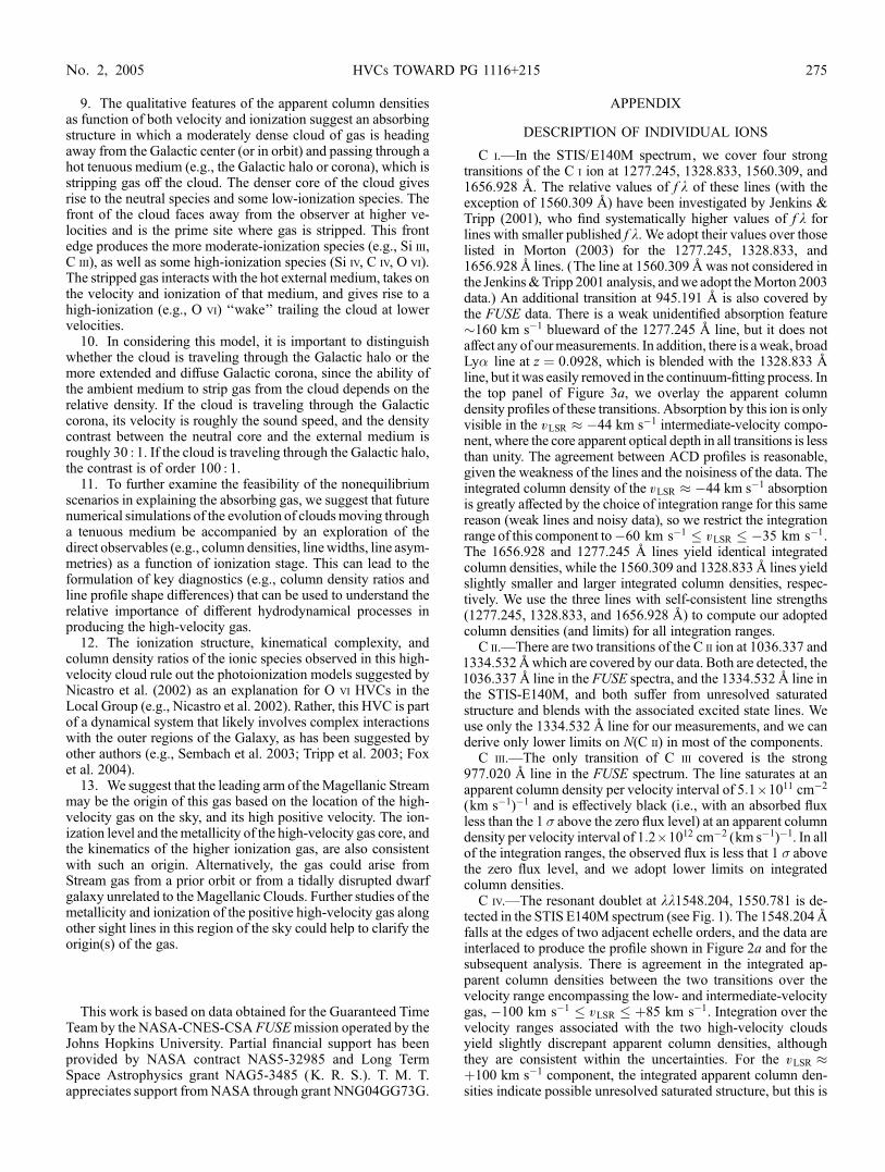
9. The qualitative features of the apparent column densitiesas function of both velocity and ionization suggest an absorbingstructure in which a moderately dense cloud of gas is headingaway from the Galactic center (or in orbit) and passing through ahot tenuous medium (e.g., the Galactic halo or corona), which isstripping gas off the cloud. The denser core of the cloud givesrise to the neutral species and some low-ionization species. Thefront of the cloud faces away from the observer at higher ve-locities and is the prime site where gas is stripped. This frontedge produces the more moderate-ionization species (e.g., Si iii,C iii), as well as some high-ionization species (Si iv, C iv, O vi).The stripped gas interacts with the hot external medium, takes onthe velocity and ionization of that medium, and gives rise to ahigh-ionization (e.g., O vi) ‘‘wake’’ trailing the cloud at lowervelocities.

10. In considering this model, it is important to distinguishwhether the cloud is traveling through the Galactic halo or themore extended and diffuse Galactic corona, since the ability ofthe ambient medium to strip gas from the cloud depends on therelative density. If the cloud is traveling through the Galacticcorona, its velocity is roughly the sound speed, and the densitycontrast between the neutral core and the external medium isroughly 30 : 1. If the cloud is traveling through the Galactic halo,the contrast is of order 100 : 1.

11. To further examine the feasibility of the nonequilibriumscenarios in explaining the absorbing gas, we suggest that futurenumerical simulations of the evolution of cloudsmoving througha tenuous medium be accompanied by an exploration of thedirect observables (e.g., column densities, linewidths, line asym-metries) as a function of ionization stage. This can lead to theformulation of key diagnostics (e.g., column density ratios andline profile shape differences) that can be used to understand therelative importance of different hydrodynamical processes inproducing the high-velocity gas.

12. The ionization structure, kinematical complexity, andcolumn density ratios of the ionic species observed in this high-velocity cloud rule out the photoionization models suggested byNicastro et al. (2002) as an explanation for O vi HVCs in theLocal Group (e.g., Nicastro et al. 2002). Rather, this HVC is partof a dynamical system that likely involves complex interactionswith the outer regions of the Galaxy, as has been suggested byother authors (e.g., Sembach et al. 2003; Tripp et al. 2003; Foxet al. 2004).

13. We suggest that the leading arm of theMagellanic Streammay be the origin of this gas based on the location of the high-velocity gas on the sky, and its high positive velocity. The ion-ization level and themetallicity of the high-velocity gas core, andthe kinematics of the higher ionization gas, are also consistentwith such an origin. Alternatively, the gas could arise fromStream gas from a prior orbit or from a tidally disrupted dwarfgalaxy unrelated to theMagellanic Clouds. Further studies of themetallicity and ionization of the positive high-velocity gas alongother sight lines in this region of the sky could help to clarify theorigin(s) of the gas.

This work is based on data obtained for the Guaranteed TimeTeam by the NASA-CNES-CSA FUSEmission operated by theJohns Hopkins University. Partial financial support has beenprovided by NASA contract NAS5-32985 and Long TermSpace Astrophysics grant NAG5-3485 (K. R. S.). T. M. T.appreciates support fromNASA through grant NNG04GG73G.

APPENDIX

DESCRIPTION OF INDIVIDUAL IONS

C i.—In the STIS/E140M spectrum, we cover four strongtransitions of the C i ion at 1277.245, 1328.833, 1560.309, and1656.928 8. The relative values of f k of these lines (with theexception of 1560.309 8) have been investigated by Jenkins &Tripp (2001), who find systematically higher values of f k forlines with smaller published f k. We adopt their values over thoselisted in Morton (2003) for the 1277.245, 1328.833, and1656.9288 lines. (The line at 1560.3098 was not considered inthe Jenkins&Tripp 2001 analysis, andwe adopt theMorton 2003data.) An additional transition at 945.191 8 is also covered bythe FUSE data. There is a weak unidentified absorption feature�160 km s�1 blueward of the 1277.245 8 line, but it does notaffect any of ourmeasurements. In addition, there is aweak, broadLy� line at z ¼ 0:0928, which is blended with the 1328.833 8line, but it was easily removed in the continuum-fitting process. Inthe top panel of Figure 3a, we overlay the apparent columndensity profiles of these transitions. Absorption by this ion is onlyvisible in the vLSR � �44 km s�1 intermediate-velocity compo-nent, where the core apparent optical depth in all transitions is lessthan unity. The agreement between ACD profiles is reasonable,given the weakness of the lines and the noisiness of the data. Theintegrated column density of the vLSR � �44 km s�1 absorptionis greatly affected by the choice of integration range for this samereason (weak lines and noisy data), so we restrict the integrationrange of this component to�60 km s�1 � vLSR � �35 km s�1.The 1656.928 and 1277.245 8 lines yield identical integratedcolumn densities, while the 1560.309 and 1328.8338 lines yieldslightly smaller and larger integrated column densities, respec-tively. We use the three lines with self-consistent line strengths(1277.245, 1328.833, and 1656.928 8) to compute our adoptedcolumn densities (and limits) for all integration ranges.

C ii.—There are two transitions of the C ii ion at 1036.337 and1334.5328which are covered by our data. Both are detected, the1036.3378 line in the FUSE spectra, and the 1334.5328 line inthe STIS-E140M, and both suffer from unresolved saturatedstructure and blends with the associated excited state lines. Weuse only the 1334.532 8 line for our measurements, and we canderive only lower limits on N(C ii) in most of the components.

C iii.—The only transition of C iii covered is the strong977.020 8 line in the FUSE spectrum. The line saturates at anapparent column density per velocity interval of 5:1 ; 1011 cm�2

(km s�1)�1 and is effectively black (i.e., with an absorbed fluxless than the 1 � above the zero flux level) at an apparent columndensity per velocity interval of 1:2 ; 1012 cm�2 (km s�1)�1. In allof the integration ranges, the observed flux is less that 1 � abovethe zero flux level, and we adopt lower limits on integratedcolumn densities.

C iv.—The resonant doublet at kk1548.204, 1550.781 is de-tected in the STIS E140M spectrum (see Fig. 1). The 1548.2048falls at the edges of two adjacent echelle orders, and the data areinterlaced to produce the profile shown in Figure 2a and for thesubsequent analysis. There is agreement in the integrated ap-parent column densities between the two transitions over thevelocity range encompassing the low- and intermediate-velocitygas, �100 km s�1 � vLSR � þ85 km s�1. Integration over thevelocity ranges associated with the two high-velocity cloudsyield slightly discrepant apparent column densities, althoughthey are consistent within the uncertainties. For the vLSR �þ100 km s�1 component, the integrated apparent column den-sities indicate possible unresolved saturated structure, but this is

HVCs TOWARD PG 1116+215 275No. 2, 2005

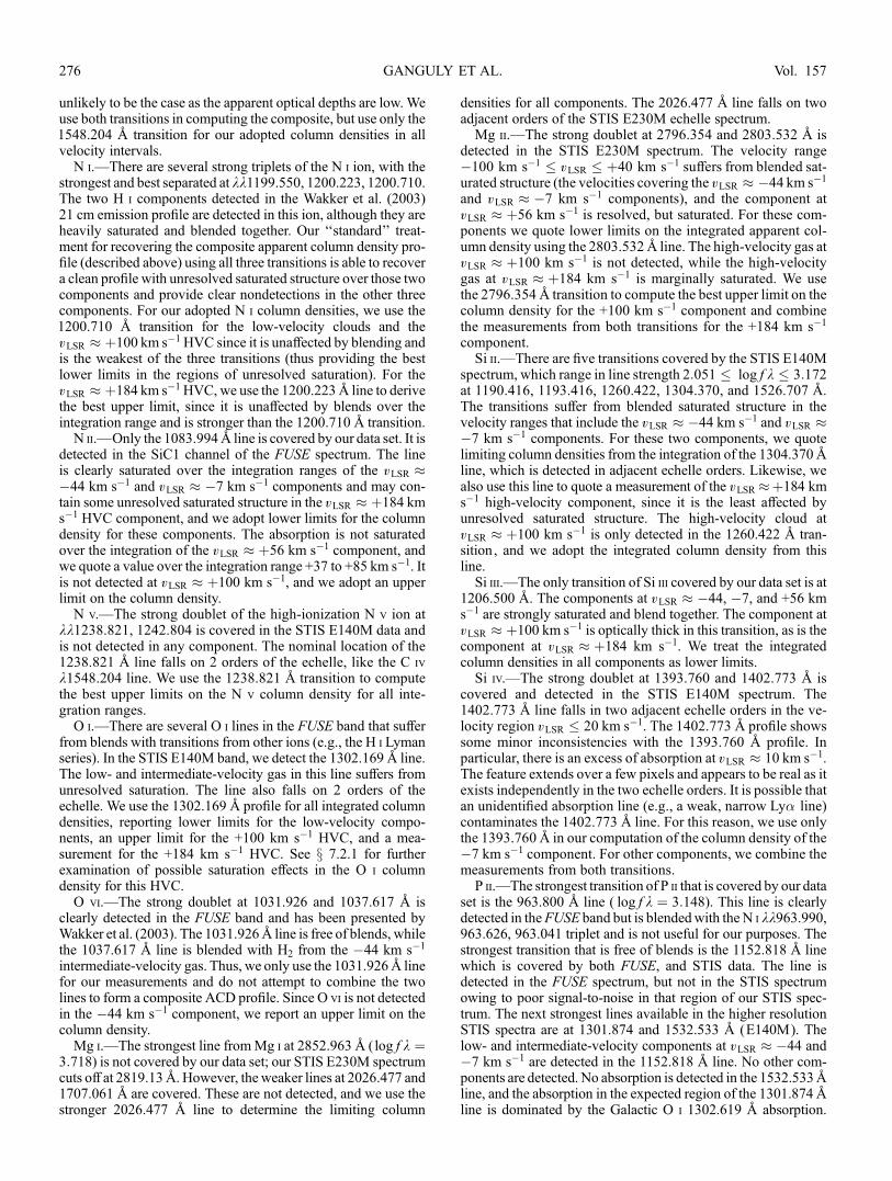
unlikely to be the case as the apparent optical depths are low. Weuse both transitions in computing the composite, but use only the1548.204 8 transition for our adopted column densities in allvelocity intervals.

N i.—There are several strong triplets of the N i ion, with thestrongest and best separated at kk1199.550, 1200.223, 1200.710.The two H i components detected in the Wakker et al. (2003)21 cm emission profile are detected in this ion, although they areheavily saturated and blended together. Our ‘‘standard’’ treat-ment for recovering the composite apparent column density pro-file (described above) using all three transitions is able to recovera clean profile with unresolved saturated structure over those twocomponents and provide clear nondetections in the other threecomponents. For our adopted N i column densities, we use the1200.710 8 transition for the low-velocity clouds and thevLSR � þ100 km s�1 HVC since it is unaffected by blending andis the weakest of the three transitions (thus providing the bestlower limits in the regions of unresolved saturation). For thevLSR � þ184 km s�1 HVC, we use the 1200.2238 line to derivethe best upper limit, since it is unaffected by blends over theintegration range and is stronger than the 1200.710 8 transition.

N ii.—Only the 1083.9948 line is covered by our data set. It isdetected in the SiC1 channel of the FUSE spectrum. The lineis clearly saturated over the integration ranges of the vLSR ��44 km s�1 and vLSR � �7 km s�1 components and may con-tain some unresolved saturated structure in the vLSR � þ184 kms�1 HVC component, and we adopt lower limits for the columndensity for these components. The absorption is not saturatedover the integration of the vLSR � þ56 km s�1 component, andwe quote a value over the integration range +37 to +85 km s�1. Itis not detected at vLSR � þ100 km s�1, and we adopt an upperlimit on the column density.

N v.—The strong doublet of the high-ionization N v ion atkk1238.821, 1242.804 is covered in the STIS E140M data andis not detected in any component. The nominal location of the1238.821 8 line falls on 2 orders of the echelle, like the C iv

k1548.204 line. We use the 1238.821 8 transition to computethe best upper limits on the N v column density for all inte-gration ranges.

O i.—There are several O i lines in the FUSE band that sufferfrom blends with transitions from other ions (e.g., the H i Lymanseries). In the STIS E140M band, we detect the 1302.1698 line.The low- and intermediate-velocity gas in this line suffers fromunresolved saturation. The line also falls on 2 orders of theechelle. We use the 1302.169 8 profile for all integrated columndensities, reporting lower limits for the low-velocity compo-nents, an upper limit for the +100 km s�1 HVC, and a mea-surement for the +184 km s�1 HVC. See x 7.2.1 for furtherexamination of possible saturation effects in the O i columndensity for this HVC.

O vi.—The strong doublet at 1031.926 and 1037.617 8 isclearly detected in the FUSE band and has been presented byWakker et al. (2003). The 1031.9268 line is free of blends, whilethe 1037.617 8 line is blended with H2 from the �44 km s�1

intermediate-velocity gas. Thus, we only use the 1031.9268 linefor our measurements and do not attempt to combine the twolines to form a composite ACD profile. Since O vi is not detectedin the �44 km s�1 component, we report an upper limit on thecolumn density.

Mg i.—The strongest line fromMg i at 2852.9638 ( log f k ¼3:718) is not covered by our data set; our STIS E230M spectrumcuts off at 2819.138. However, the weaker lines at 2026.477 and1707.061 8 are covered. These are not detected, and we use thestronger 2026.477 8 line to determine the limiting column

densities for all components. The 2026.477 8 line falls on twoadjacent orders of the STIS E230M echelle spectrum.Mg ii.—The strong doublet at 2796.354 and 2803.532 8 is

detected in the STIS E230M spectrum. The velocity range�100 km s�1 � vLSR � þ40 km s�1 suffers from blended sat-urated structure (the velocities covering the vLSR � �44 km s�1

and vLSR � �7 km s�1 components), and the component atvLSR � þ56 km s�1 is resolved, but saturated. For these com-ponents we quote lower limits on the integrated apparent col-umn density using the 2803.5328 line. The high-velocity gas atvLSR � þ100 km s�1 is not detected, while the high-velocitygas at vLSR � þ184 km s�1 is marginally saturated. We usethe 2796.3548 transition to compute the best upper limit on thecolumn density for the +100 km s�1 component and combinethe measurements from both transitions for the +184 km s�1

component.Si ii.—There are five transitions covered by the STIS E140M

spectrum, which range in line strength 2:051 � log f k � 3:172at 1190.416, 1193.416, 1260.422, 1304.370, and 1526.707 8.The transitions suffer from blended saturated structure in thevelocity ranges that include the vLSR � �44 km s�1 and vLSR ��7 km s�1 components. For these two components, we quotelimiting column densities from the integration of the 1304.3708line, which is detected in adjacent echelle orders. Likewise, wealso use this line to quote a measurement of the vLSR �þ184 kms�1 high-velocity component, since it is the least affected byunresolved saturated structure. The high-velocity cloud atvLSR � þ100 km s�1 is only detected in the 1260.422 8 tran-sition, and we adopt the integrated column density from thisline.Si iii.—The only transition of Si iii covered by our data set is at

1206.500 8. The components at vLSR � �44, �7, and +56 kms�1 are strongly saturated and blend together. The component atvLSR � þ100 km s�1 is optically thick in this transition, as is thecomponent at vLSR � þ184 km s�1. We treat the integratedcolumn densities in all components as lower limits.Si iv.—The strong doublet at 1393.760 and 1402.773 8 is

covered and detected in the STIS E140M spectrum. The1402.773 8 line falls in two adjacent echelle orders in the ve-locity region vLSR � 20 km s�1. The 1402.773 8 profile showssome minor inconsistencies with the 1393.760 8 profile. Inparticular, there is an excess of absorption at vLSR � 10 km s�1.The feature extends over a few pixels and appears to be real as itexists independently in the two echelle orders. It is possible thatan unidentified absorption line (e.g., a weak, narrow Ly� line)contaminates the 1402.773 8 line. For this reason, we use onlythe 1393.7608 in our computation of the column density of the�7 km s�1 component. For other components, we combine themeasurements from both transitions.P ii.—The strongest transition of P ii that is covered by our data

set is the 963.800 8 line ( log f k ¼ 3:148). This line is clearlydetected in theFUSE band but is blendedwith the N i kk963.990,963.626, 963.041 triplet and is not useful for our purposes. Thestrongest transition that is free of blends is the 1152.818 8 linewhich is covered by both FUSE, and STIS data. The line isdetected in the FUSE spectrum, but not in the STIS spectrumowing to poor signal-to-noise in that region of our STIS spec-trum. The next strongest lines available in the higher resolutionSTIS spectra are at 1301.874 and 1532.533 8 (E140M). Thelow- and intermediate-velocity components at vLSR � �44 and�7 km s�1 are detected in the 1152.818 8 line. No other com-ponents are detected. No absorption is detected in the 1532.5338line, and the absorption in the expected region of the 1301.8748line is dominated by the Galactic O i 1302.619 8 absorption.


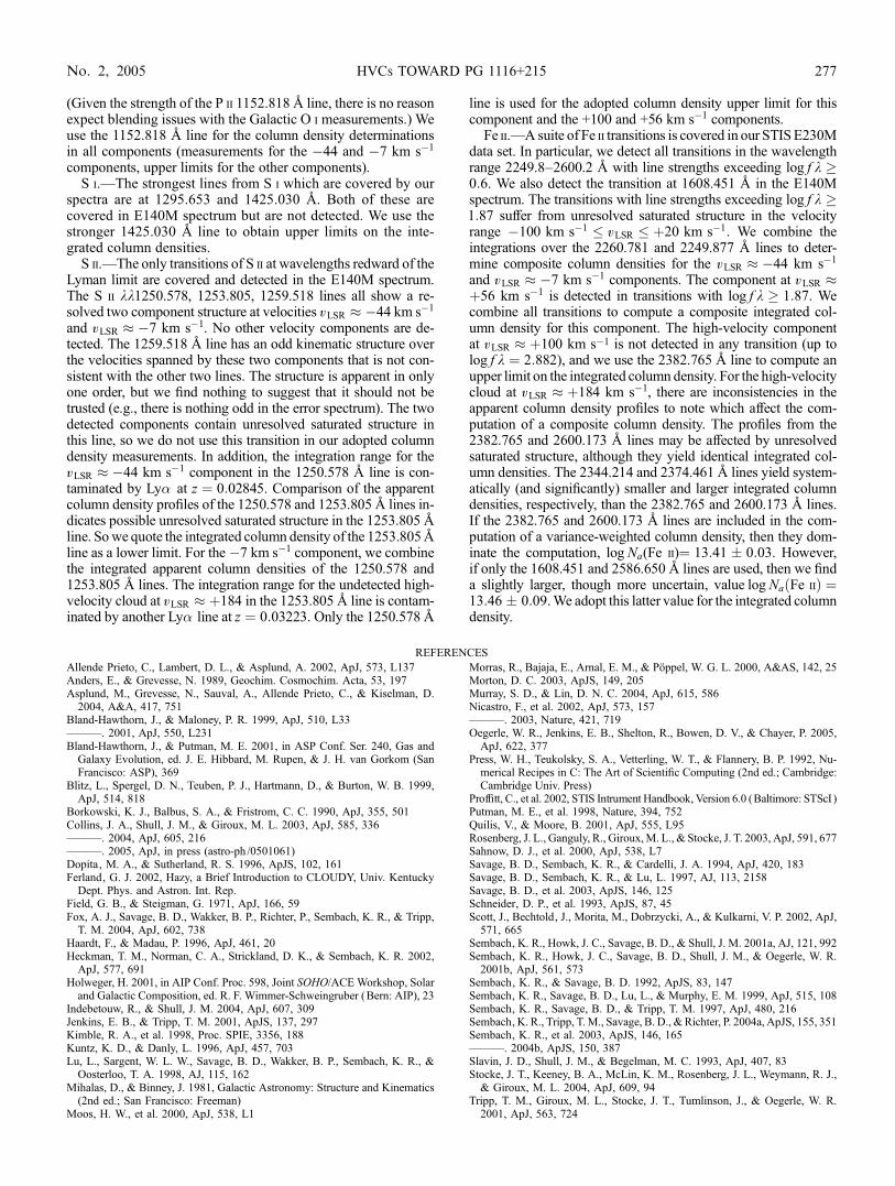
(Given the strength of the P ii 1152.8188 line, there is no reasonexpect blending issues with the Galactic O i measurements.) Weuse the 1152.818 8 line for the column density determinationsin all components (measurements for the �44 and �7 km s�1

components, upper limits for the other components).S i.—The strongest lines from S i which are covered by our

spectra are at 1295.653 and 1425.030 8. Both of these arecovered in E140M spectrum but are not detected. We use thestronger 1425.030 8 line to obtain upper limits on the inte-grated column densities.

S ii.—The only transitions of S ii at wavelengths redward of theLyman limit are covered and detected in the E140M spectrum.The S ii kk1250.578, 1253.805, 1259.518 lines all show a re-solved two component structure at velocities vLSR � �44 km s�1

and vLSR � �7 km s�1. No other velocity components are de-tected. The 1259.518 8 line has an odd kinematic structure overthe velocities spanned by these two components that is not con-sistent with the other two lines. The structure is apparent in onlyone order, but we find nothing to suggest that it should not betrusted (e.g., there is nothing odd in the error spectrum). The twodetected components contain unresolved saturated structure inthis line, so we do not use this transition in our adopted columndensity measurements. In addition, the integration range for thevLSR � �44 km s�1 component in the 1250.578 8 line is con-taminated by Ly� at z ¼ 0:02845. Comparison of the apparentcolumn density profiles of the 1250.578 and 1253.8058 lines in-dicates possible unresolved saturated structure in the 1253.8058line. Sowe quote the integrated column density of the 1253.8058line as a lower limit. For the�7 km s�1 component, we combinethe integrated apparent column densities of the 1250.578 and1253.805 8 lines. The integration range for the undetected high-velocity cloud at vLSR � þ184 in the 1253.8058 line is contam-inated by another Ly� line at z ¼ 0:03223. Only the 1250.5788

line is used for the adopted column density upper limit for thiscomponent and the +100 and +56 km s�1 components.

Fe ii.—A suite of Fe ii transitions is covered in our STISE230Mdata set. In particular, we detect all transitions in the wavelengthrange 2249.8–2600.2 8 with line strengths exceeding log f k �0:6. We also detect the transition at 1608.451 8 in the E140Mspectrum. The transitions with line strengths exceeding log f k �1:87 suffer from unresolved saturated structure in the velocityrange �100 km s�1 � vLSR � þ20 km s�1. We combine theintegrations over the 2260.781 and 2249.877 8 lines to deter-mine composite column densities for the vLSR � �44 km s�1

and vLSR � �7 km s�1 components. The component at vLSR �þ56 km s�1 is detected in transitions with log f k � 1:87. Wecombine all transitions to compute a composite integrated col-umn density for this component. The high-velocity componentat vLSR � þ100 km s�1 is not detected in any transition (up tolog f k ¼ 2:882), and we use the 2382.765 8 line to compute anupper limit on the integrated column density. For the high-velocitycloud at vLSR � þ184 km s�1, there are inconsistencies in theapparent column density profiles to note which affect the com-putation of a composite column density. The profiles from the2382.765 and 2600.173 8 lines may be affected by unresolvedsaturated structure, although they yield identical integrated col-umn densities. The 2344.214 and 2374.4618 lines yield system-atically (and significantly) smaller and larger integrated columndensities, respectively, than the 2382.765 and 2600.173 8 lines.If the 2382.765 and 2600.173 8 lines are included in the com-putation of a variance-weighted column density, then they dom-inate the computation, log Na(Fe ii)¼ 13:41 � 0:03. However,if only the 1608.451 and 2586.650 8 lines are used, then we finda slightly larger, though more uncertain, value log NaðFe iiÞ ¼13:46 � 0:09.We adopt this latter value for the integrated columndensity.

REFERENCES

Allende Prieto, C., Lambert, D. L., & Asplund, A. 2002, ApJ, 573, L137Anders, E., & Grevesse, N. 1989, Geochim. Cosmochim. Acta, 53, 197Asplund, M., Grevesse, N., Sauval, A., Allende Prieto, C., & Kiselman, D.2004, A&A, 417, 751

Bland-Hawthorn, J., & Maloney, P. R. 1999, ApJ, 510, L33———. 2001, ApJ, 550, L231Bland-Hawthorn, J., & Putman, M. E. 2001, in ASP Conf. Ser. 240, Gas andGalaxy Evolution, ed. J. E. Hibbard, M. Rupen, & J. H. van Gorkom (SanFrancisco: ASP), 369

Blitz, L., Spergel, D. N., Teuben, P. J., Hartmann, D., & Burton, W. B. 1999,ApJ, 514, 818

Borkowski, K. J., Balbus, S. A., & Fristrom, C. C. 1990, ApJ, 355, 501Collins, J. A., Shull, J. M., & Giroux, M. L. 2003, ApJ, 585, 336———. 2004, ApJ, 605, 216———. 2005, ApJ, in press (astro-ph /0501061)Dopita, M. A., & Sutherland, R. S. 1996, ApJS, 102, 161Ferland, G. J. 2002, Hazy, a Brief Introduction to CLOUDY, Univ. KentuckyDept. Phys. and Astron. Int. Rep.

Field, G. B., & Steigman, G. 1971, ApJ, 166, 59Fox, A. J., Savage, B. D., Wakker, B. P., Richter, P., Sembach, K. R., & Tripp,T. M. 2004, ApJ, 602, 738

Haardt, F., & Madau, P. 1996, ApJ, 461, 20Heckman, T. M., Norman, C. A., Strickland, D. K., & Sembach, K. R. 2002,ApJ, 577, 691

Holweger, H. 2001, in AIP Conf. Proc. 598, Joint SOHO/ACE Workshop, Solarand Galactic Composition, ed. R. F. Wimmer-Schweingruber (Bern: AIP), 23

Indebetouw, R., & Shull, J. M. 2004, ApJ, 607, 309Jenkins, E. B., & Tripp, T. M. 2001, ApJS, 137, 297Kimble, R. A., et al. 1998, Proc. SPIE, 3356, 188Kuntz, K. D., & Danly, L. 1996, ApJ, 457, 703Lu, L., Sargent, W. L. W., Savage, B. D., Wakker, B. P., Sembach, K. R., &Oosterloo, T. A. 1998, AJ, 115, 162

Mihalas, D., & Binney, J. 1981, Galactic Astronomy: Structure and Kinematics(2nd ed.; San Francisco: Freeman)

Moos, H. W., et al. 2000, ApJ, 538, L1

Morras, R., Bajaja, E., Arnal, E. M., & Poppel, W. G. L. 2000, A&AS, 142, 25Morton, D. C. 2003, ApJS, 149, 205Murray, S. D., & Lin, D. N. C. 2004, ApJ, 615, 586Nicastro, F., et al. 2002, ApJ, 573, 157———. 2003, Nature, 421, 719Oegerle, W. R., Jenkins, E. B., Shelton, R., Bowen, D. V., & Chayer, P. 2005,ApJ, 622, 377

Press, W. H., Teukolsky, S. A., Vetterling, W. T., & Flannery, B. P. 1992, Nu-merical Recipes in C: The Art of Scientific Computing (2nd ed.; Cambridge:Cambridge Univ. Press)

Proffitt, C., et al. 2002, STIS Intrument Handbook, Version 6.0 (Baltimore: STScI )Putman, M. E., et al. 1998, Nature, 394, 752Quilis, V., & Moore, B. 2001, ApJ, 555, L95Rosenberg, J. L., Ganguly, R., Giroux,M. L., & Stocke, J. T. 2003, ApJ, 591, 677Sahnow, D. J., et al. 2000, ApJ, 538, L7Savage, B. D., Sembach, K. R., & Cardelli, J. A. 1994, ApJ, 420, 183Savage, B. D., Sembach, K. R., & Lu, L. 1997, AJ, 113, 2158Savage, B. D., et al. 2003, ApJS, 146, 125Schneider, D. P., et al. 1993, ApJS, 87, 45Scott, J., Bechtold, J., Morita, M., Dobrzycki, A., & Kulkarni, V. P. 2002, ApJ,571, 665

Sembach, K. R., Howk, J. C., Savage, B. D., & Shull, J. M. 2001a, AJ, 121, 992Sembach, K. R., Howk, J. C., Savage, B. D., Shull, J. M., & Oegerle, W. R.2001b, ApJ, 561, 573

Sembach, K. R., & Savage, B. D. 1992, ApJS, 83, 147Sembach, K. R., Savage, B. D., Lu, L., & Murphy, E. M. 1999, ApJ, 515, 108Sembach, K. R., Savage, B. D., & Tripp, T. M. 1997, ApJ, 480, 216Sembach, K. R., Tripp, T.M., Savage, B. D., & Richter, P. 2004a, ApJS, 155, 351Sembach, K. R., et al. 2003, ApJS, 146, 165———. 2004b, ApJS, 150, 387Slavin, J. D., Shull, J. M., & Begelman, M. C. 1993, ApJ, 407, 83Stocke, J. T., Keeney, B. A., McLin, K. M., Rosenberg, J. L., Weymann, R. J.,& Giroux, M. L. 2004, ApJ, 609, 94

Tripp, T. M., Giroux, M. L., Stocke, J. T., Tumlinson, J., & Oegerle, W. R.2001, ApJ, 563, 724

HVCs TOWARD PG 1116+215 277No. 2, 2005

Tripp, T. M., Lu, L., & Savage, B. D. 1998, ApJ, 508, 200Tripp, T. M., & Savage, B. D. 2000, ApJ, 542, 42Tripp, T. M., et al. 2002, ApJ, 575, 697———. 2003, AJ, 125, 3122Wakker, B. P. 2001, ApJS, 136, 463———. 2004, Ap&SS, 289, 381Wakker, B. P., et al. 2003, ApJS, 146, 1

Weiner, B. J., Vogel, S. N., & Williams, T. B. 2002, in ASP Conf. Ser. 254,Extragalactic Gas at Low Redshift, ed. J. S. Mulchaey & J. Stocke (SanFrancisco: ASP), 256

Welty, D. E., Frisch, P. C., Sonneborn, G., & York, D. G. 1999, ApJ, 512, 636Welty, D. E., Lauroesch, J. T., Blades, J. C., Hobbs, L. M., & York, D. G. 1997,ApJ, 489, 672

Woodgate, B. E., et al. 1998, PASP, 110, 1183

GANGULY ET AL.278

Documents

HIGHLY IONIZED GAS IN THE GALACTIC HALO AND THE HIGH-VELOCITY