Consist

ent *Complete *

Well D

ocumented*Easyt

oR

euse* *

Evaluated

*ECOOP*

Artifact

*AEC

Higher-Order Demand-Driven Program AnalysisZachary Palmer1 and Scott F. Smith2

1 Swarthmore CollegeSwarthmore, PA, USAzachary.palmer@swarthmore.edu

2 The Johns Hopkins UniversityBaltimore, MD, USAscott@cs.jhu.edu

AbstractWe explore a novel approach to higher-order program analysis that brings ideas of on-demandlookup from first-order CFL-reachability program analyses to higher-order programs. The anal-ysis needs to produce only a control-flow graph; it can derive all other information includingvalues of variables directly from the graph. Several challenges had to be overcome, including howto build the control-flow graph on-the-fly and how to deal with non-local variables in functions.The resulting analysis is flow- and context-sensitive with a provable polynomial-time bound.The analysis is formalized and proved correct and terminating, and an initial implementation isdescribed.

1998 ACM Subject Classification F.3.2. Semantics of Programming Languages

Keywords and phrases functional programming, program analysis, polynomial-time, demand-driven, flow-sensitive, context-sensitive

Digital Object Identifier 10.4230/LIPIcs.xxx.yyy.p

1 Introduction

Flow analysis for imperative first-order programs is a well-known and straightforward pro-cess. Before the analysis starts, it is known which functions are being invoked at each callsite in the source program. This is possible because, in absence of higher-order functions,potential control flow is determined immediately from the structure of the program. So, forfirst-order programs, it is possible to directly build a fixed control flow graph (CFG) whereeach edge in the CFG points to a potential next program point. The program analysis thencan monotonically accumulate information about what values program variables could takeon at each program point, propagating information along this fixed CFG.

Forward higher-order program analysis

In languages with higher-order functions, program analysis is much more challenging: it isno longer obvious which functions may be invoked at each call site. The program’s data flowdetermines which functions appear at the call site, in turn influencing the program’s controlflow. Accurate analyses of programs with higher-order functions must therefore computedata- and control-flow information simultaneously [12, 16].

Higher-order program analyses are generally based on abstract interpretations [2]; suchanalyses define a finite-state abstraction of the operational semantics transition relation tosoundly approximate the program’s runtime behavior. The resulting analysis has the samegeneral structure as the operational semantics it was based on: program points, environ-ments, stacks, stores, and addresses are replaced with abstract counterparts which have

© Zachary E. Palmer and Scott F. Smith;licensed under Creative Commons License CC-BY

Conference title on which this volume is based on.Editors: Billy Editor and Bill Editors; pp. 1–25

Leibniz International Proceedings in InformaticsSchloss Dagstuhl – Leibniz-Zentrum für Informatik, Dagstuhl Publishing, Germany

2 Higher-Order Demand-Driven Program Analysis

finite cardinality, “hobbling” the full operational semantics of the language to guaranteetermination of the analysis [13]. A sound analysis will visit the (finitely many) abstractcounterparts of all reachable concrete program states, producing a finite automaton repre-senting all potential program runs.

We use the term “forward analyses” to refer to standard higher-order program analyses,to emphasize how they propagate data forward through the program in the same manneras an operational semantics does. All abstract interpretation based higher-order programanalyses, including [12, 16, 22, 13, 27, 8, 15, 3], are forward analyses.

Since each node is an abstract state and there can be a great many combinations ofdata for environment or store, even the finitized abstract state space can be very large. Forthis reason, any practical analysis must compress the total number of states. Typically, theprogram counter is preserved. One standard compression, store widening, replaces the storein each each abstract program state with a single global store; this global store is then theunion of all the individual stores.

Store widening is effective in compressing the abstract state set but tends to give toolittle precision. For example, function polymorphism which is present before store wideningmay be lost as the parameters to the calls of a given function in each program state areunioned together. Store widening also generally loses any so-called flow sensitivity, where agiven (often stateful) variable can take on different values at different points.

So, other methods are employed to recover expressiveness without a full store in eachabstract state. One method is polyvariance, such as in kCFA [22] for k > 0, where eachfunction parameter gets unique addresses relative to the k most recent stack frames. Anothermethod is call-return alignment: the analysis uses a stack internally to return only to thecall site of the particular call being analyzed [26]. Call-return alignment also gives some, butnot all, of the power of polyvariance. One alternative to store widening is abstract garbagecollection [14], which also limits the number of abstract states: the store is not widened,but an analysis-time analogue of run-time garbage collection removes inaccessible bindingsfrom the store. Abstract GC preserves flow-sensitivity, but this technique is still susceptibleto an explosion in analysis states for programs with nontrivial amounts of persistent dataas each configuration of this data represents another abstract program state to consider.

A demand-driven approach to higher-order programs

In this paper, we explore a fundamentally different approach to higher-order program analy-sis which does not proceed by finitizing an operational semantics. Rather than pushing dataforward as in an operational semantics, the analysis looks up data on demand. This lookupwalks backward along the control flow from the point at which a variable’s value is neededto the point at which the variable was most recently defined. Actual values never need tobe pushed forward so, in some sense, lookup is lazier than a standard lazy interpreter.

CFL-reachability analyses [6] have shown how demand-driven variable lookup is possi-ble in first-order program analyses. In comparison to forward analyses, the demand-drivenapproach has potential for better performance: the aforementioned optimizations are un-necessary as no store is propagated forward through the analysis. CFL-reachability is afirst-order analysis, where the CFG is already known and where there are no non-localvariables in functions. Demand-driven lookup is applied to higher-order languages in [18],but in the a context of a flow-insensitive type-based analysis with other restrictions. Togenerally apply this technique to higher-order programs, we must have (1) a technique forconstructing the CFG in tandem with the data flow analysis and (2) a strategy for handlingnon-local variables.

Z. Palmer and S. F. Smith 3

In this paper, we solve these two problems to produce a higher-order Demand-DrivenProgram Analysis (DDPA). The CFG is constructed incrementally just as in a forwardhigher-order program analysis. Unlike a forward analysis, we only need to construct theCFG; there is no abstracted environment/store/etc as all of the variable lookup happens inreverse by following CFG edges backwards. To deal with non-local variables in functions,we develop a novel reverse lookup process that is related to how access links are used in acompiler to look up non-local variables: we find the definition of the function itself and lookup the variable from there. For added precision, we incorporate call-return alignment fromCFL-reachability [21, 20] and pushdown higher-order flow analyses [26, 8].

Contrast with forward analyses

During the course of DDPA, each variable lookup occurs relative to a particular point in the(partial) control flow graph where the variable is used; this makes flow-sensitivity a naturalcomponent of DDPA. In forward higher-order analyses, such flow-sensitivity is expensivesince it prohibits common performance-enhancing techniques such as store widening. Ab-stract garbage collection, an aforementioned alternative to store widening, prunes the storessignificantly but produces many states for persistent data. Additionally, there is no needfor explicit polyvariance in DDPA: the combination of call-return alignment and non-locallookup achieves the full effect of polyvariance without an explicit polyvariance model a lakCFA. DDPA appears to compare favorably to forward analyses: it has the simultaneousbenefits of store widening (we have no per-node store), abstract garbage collection (demand-driven lookup prevents the generation of garbage), call-return alignment (the one featurewe directly adopt) and polyvariance (which is subsumed by our call-return alignment givenour novel non-local variable lookup mechanism). Forward analyses cannot combine all thesefeatures because abstract GC is ineffective in the presence of store widening [8].

In theory, DDPA has minimal requirements on run-time data structures: the only re-quired data structure is the CFG, which is minuscule compared to the formal treatment offorward analysis. In practice, an efficient DDPA implementation requires significant cachingstructures which are similar to fragments of an abstract store in a forward analysis. Wedo not assert DDPA to be a strictly better form of program analysis, only a substantiallydifferent one with different trade-offs and worthy of study.

In terms of technical overhead, DDPA has the advantage of naturally scaling up to aflow-, path-, and context-sensitive analysis while preserving a relatively compact formalspecification. On the other hand, reverse lookup is a different process than the original(forward) operational semantics and requires a major re-thinking about program flow; aforward analysis can to some degree be “read off the operational semantics” [25, 13].

We have completed a proof-of-concept implementation of DDPA, described in Section 6,and include it as an artifact archived with the paper. The implementation builds a push-down automaton (PDA) and variable lookup questions can be cast as reachability questionsin the PDA. This implementation has not been optimized but it confirms that the analysishas the expected behavior on examples.

Paper outline

Section 2 presents an example-driven description of the main features of the analysis. Section3 gives the full details, and Section 4 establishes its soundness relative to an operationalsemantics. Section 5 defines extensions for full records, path-sensitivity, and state. Section6 describes the implementation. Section 7 covers related work. We conclude in Section 8.

4 Higher-Order Demand-Driven Program Analysis

e ::= [c, . . .] expressionsc ::= x = b clausesb ::= v | x | x x | x ~ p ? f : f clause bodiesx variables

E ::= [x = v, . . .] environments

v ::= r | f valuesr ::= {`, . . .} recordsf ::= fun x -> ( e ) functionsp ::= r patterns

Figure 1 Expression Grammar

1 f = fun x -> ( # λx.(λy.y)x2 i = fun a -> (3 r2 = a4 );5 r = i x;6 n0 = r;7 );8 x1 = {y};9 z1 = f x1; # evaluates to {y}

10 x2 = {n};11 z2 = f x2; # evaluates to {n}

f x1 z1 x2 z2Start End

xz1↓= x1 z1z1↑

= n0

i n0r

1

11

1

ar↓=x r2 rr↑

=r22

2 22

xz2↓= x2 z2z2↑

= n03

33

3

Figure 2 Invocation Example: ANF Figure 3 Invocation Example: Analysis

2 Overview of the Analysis

This section informally presents DDPA by example.

2.1 A Simple Language

For a given program, our objective is to establish the possible execution paths that theprogram will take. We encode this information in the form of a CFG, more precisely as ahappens-before relation c << c′: program point c related to c′ means there may be controlflow from c to c′.

We use a simple functional language defined in Figure 1. To make it easier to keeptrack of program points and operation sequencing, we restrict our language syntax to ashallow A-normal form (ANF) [5]. We further restrict all variables to be unique; this ensuresthat clauses c themselves denote program points. (Notation: lists are written [g1, . . . , gn],and || denotes list concatenation. We may overload as g1 ||[g2, g3] = [g1, g2, g3] when it isunambiguous.)

The operational semantics of this (eager) language are straightforward and are givenin Section 4.1. Note that we have a degenerate form of record with label componentsonly; this restriction is made to simplify the formalism and we relax this restriction in theimplementation. Case analysis is written x ~ p ? f1 : f2; we execute f1 with x as argument ifthe value of x matches the pattern p, and f2 with x as argument otherwise.

2.2 The Basic Analysis

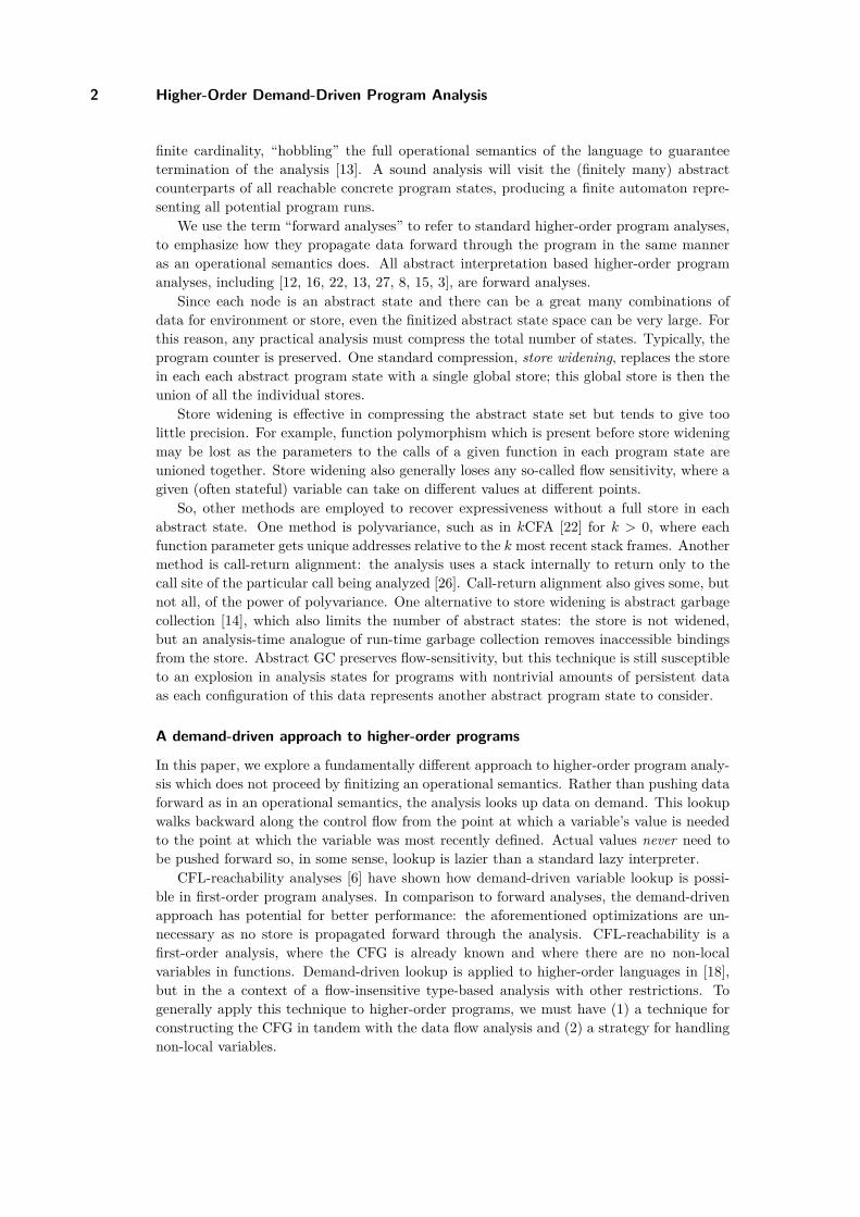
Consider the program in Figure 2. Note that f is just a fancy identity function used to helpillustrate the analysis, and that clause n0 is a “no-op”: it is present only to help clarify thediagrams.

Z. Palmer and S. F. Smith 5

The analysis begins by constraining the top-level clauses to happen in order: f, x1, z1,x2, and then z2. For technical reasons, we also add distinguished Start and End nodes.

Figure 3 shows the completed analysis; up to now we have only described the bottomrow. Focusing only on that row for now, the solid arrows ( ) represent nodes ordered by<< in the source program, and indicate what we know about control flow at the beginningof the analysis: only that control can move from each clause to the next. As shorthand, weidentify each clause by the unique variable it assigns; thus, the green node labeled x1 refersto line 8 in Figure 2. Green nodes are immediate clauses and gray nodes are call sites.

2.2.1 Adding control flows for function calls

To elaborate the call graph, we must connect each call site to any function body invoked atthat call site. Proceeding forward on the control flow from the program start, the first callsite (gray node) is node z1. The dotted edges ( ) annotated with the number “1” representcontrol passing from call site z1 to the start of the body of f (the i, r, n0 clauses), and fromthe end of the function body back to z1. Note that the wires in fact run “around” the callsite in the figure, going out the predecessor of z1 and back to the successor. This reflectshow a function inlining would work. (Aside: both and edges define << relationshipsbetween program points; the two edge sorts are used for illustration only.)

Additionally, the call adds two new intermediate nodes: x=x1 represents copying theargument x1 at the call site into the function f’s parameter, while z1=n0 represents copyingthe result of the function into the variable defined at the call site. These nodes are markedwith annotations to indicate their call site and purpose; z1↓, for instance, indicates a pa-rameter passed in from the z1 call site. All of the information in these new nodes can infact be inferred from context since all values are unique given a (call site, function) pair. Inother words, the happens-before relation is isomorphic to the call graph.

Continuing with the analysis: now that the body of f has been wired in, the call siter can execute, adding two orange wiring nodes and the corresponding “2” flows. The “3”flows are similarly added when we elaborate z2.

2.2.2 Variable lookup as reverse walk

In the description above, we glossed over how variable lookup occurs: for each call site, weneeded to look up the particular functions to invoke and this can be nontrivial in a higher-order language. The clause z1 invokes f, and all potential definitions of f need to be wiredto the call site. This particular case is simple since f obviously has only one value.

In general, variable lookup is contextual: lookup starts at the clause where the variableis being used and proceeds backwards in time with respect to the control flow to find themost recent value. This approach to lookup is related to the demand-driven optimizationsof first-order CFL-reachability analyses [6].

For a less trivial example, let us look up x from the perspective of r’s defining clausein line 5. Walking back though the graph from r, there are two definitions of x reached:x=x1 and x=x2. Since x1/x2 are not concrete values, lookup proceeds by looking up thosevariables, respectively. Ultimately, x has final value set {{y}, {n}}, the set of arguments thefunction was invoked on.

Since variable lookup always starts at the node representing the redex where the variableis used, we obtain a flow-sensitive analysis by default. Note that the specification of lookuptraverses all the way back to the original definition every time; for example, in looking up x

6 Higher-Order Demand-Driven Program Analysis

we needed to look up x=x1 and we then needed to continue back to x1’s original definition.An efficient implementation should cache, but that is orthogonal to the specification.

2.3 Constraining lookup to reasonable call stacksThe above description of a simple lookup leaves out an important refinement in DDPA: itis possible to rule out variable lookup search paths on which calls and returns do not align,because such a path corresponds to no program execution. To show the incompletenessof lookup as described thus far, consider how lookup would find values for z2 from theperspective of the end of the program. To find z2, we proceed back on the control flow toz2=n0 (recall how the call site itself is dead code after all calls have been wired in), at whichpoint the search is now for the value of n0; continuing back we reach n0=r and proceed bylooking up r from node n0, and so on until we are looking up x from node i. Here, there aretwo paths, to either x=x1 or x=x2. So, we take both paths and union the result, obtaining{{y}, {n}}. This is clearly a loss of precision: {y} cannot appear as the argument of call sitez2 at runtime. But, looking at the overall path we took above in this spurious lookup, wewalked back into the function via the z2 call site and came out of the front of the functionto the z1 call site. This is a non-sensical program execution path since the call and returnsite are not aligned.

The annotations z1↓ / z1↑ on the wiring nodes indicate a call into and return fromcall site z1, respectively, and are used to filter out these spurious paths. On any lookuppath the wiring annotations must pair correctly; that is, one may only visit a z1↓ node ifa corresponding z1↑ node was visited. We track these pairings using an abstract call stackto verify they obey a reasonable call-return discipline. The idea of call-return alignment istaken from CFL-reachability [21, 20] and higher-order pushdown analyses [26, 8].

Note that the above analysis exhibits polyvariant behavior: different invocations of thesame function are not analyzed uniformly. Polyvariance is commonly achieved by copying,kCFA being a canonical example [16]. In DDPA, polyvariance can be achieved solely bycall-return alignment, unlike [26, 8] – stack alignment in these analyses only aligns variableslocal to the function body, whereas DDPA also aligns non-locals; the subtleties of non-locallookup are covered next.

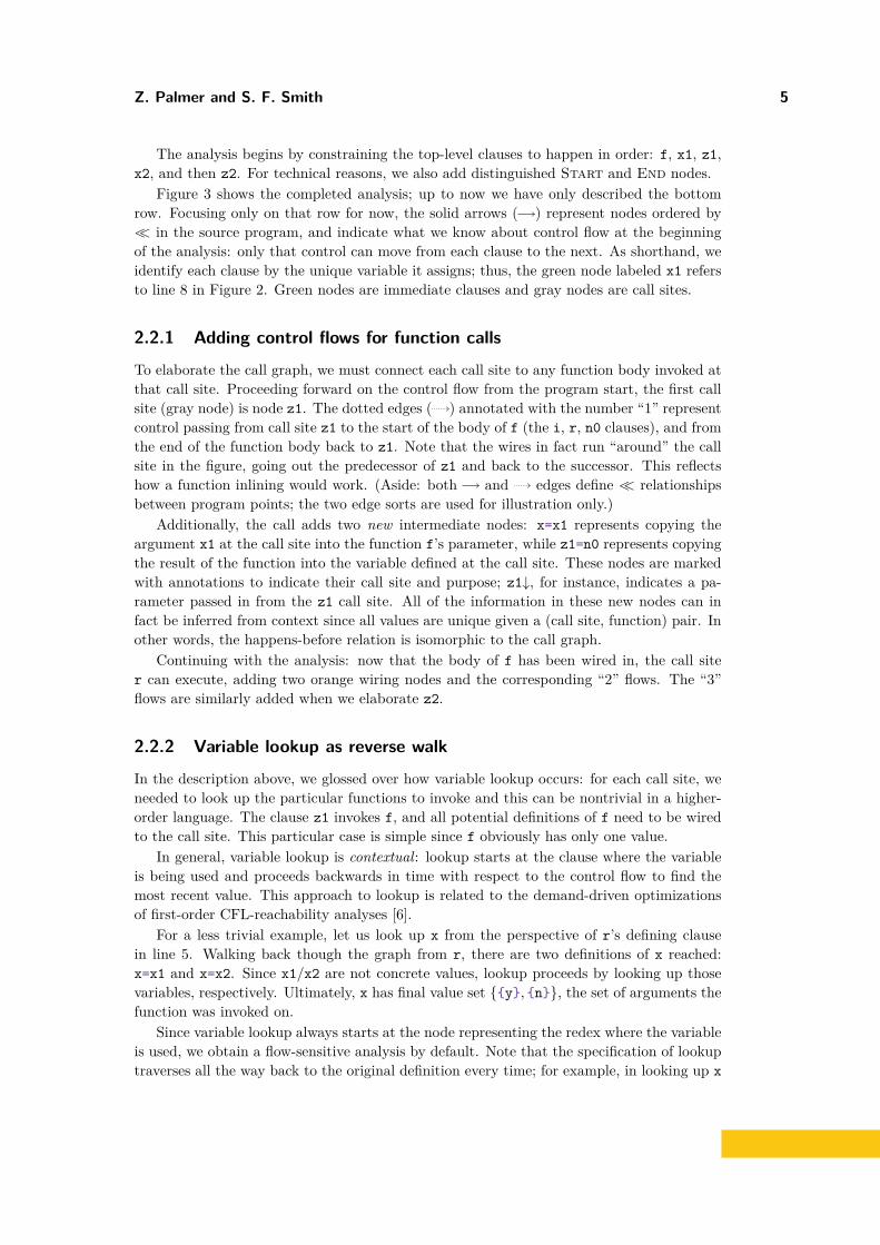
2.4 Looking up Non-Local VariablesSo far, our examples of lookup have been restricted to local variables. However, the abovelookup process does not accurately reflect how non-local variables are bound: if non-localvariables were handled in the same way, lookup would give non-locals a dynamically scopedsemantics. To see why, consider the code in Figure 4 and its graph in Figure 5. If we lookup the value of z from the end of the program, we find ourselves asking for the values ofv at the wiring of j=e. Proceeding as described above, j does not match v and we wouldattempt to find a value for v at the e clause. This leads us to the clause v=b, which in turngives us just the value {b}. This would be unsound as it is not consistent with run-timebehavior.

To give lexical scoping semantics, the lookup function must be modified. Lexical scopingmeans we want the values of non-local variables at the point which the function containingthem was itself declared, so we proceed by first locating the function definition and thenresuming our search for the value of the variable. This is similar to the access link method ofnon-local lookup in a compiler implementation. In the example above, the pivotal decisionis made when finding values of v when we have searched through the whole body of the

Z. Palmer and S. F. Smith 7

1 k = fun v -> ( # λx.λy.x2 k0 = fun j -> ( r = v; );3 );4 a = {a};5 f = k a; # λy.{a}6 b = {b};7 g = k b; # λy.{b}8 e = {};9 z = f e; # evaluates to {a}

k a f b g e z

Start End

k0vf↓=a ff↑

=k0

vg↓=b gg↑

=k0 rjz↓

=e

zz↑=r

Figure 4 Non-Local Variable: ANF Figure 5 Non-Local Variable: Analysis

function in lines 2-4 and arrived at the argument wiring j=e. From the annotation z↓ onthis node, we can deduce that we are leaving the current function which was called fromsite z. Since we have not yet found v, it must be a non-local. So, we then delay our searchfor v, examine the call site z (appearing in the wiring annotation), and look up the functioninvoked at that point; here, this means to search for f starting from e. This search leads usthrough f=k0 to k0, the point at which the function was originally defined, and from herethe search for v can soundly resume. Using this approach, the lookup of z from the end ofthe program yields {a}.

The general case of non-local lookup chains on the above idea, since the defining functioncould itself be non-locally defined. The chain is up the lexical scoping structure, so its lengthis bound by program size.

2.5 Looking up Higher-Order FunctionsThe analysis described thus far also does not deal well with the case of multiple functionsshowing up at a call site – it does not take in account which functions are actually available.Consider the code example in Figure 6.

We would like a search for rb from the End to conclude {{b}}, the run-time result. In theprocess of trying to answer that question, the analysis eventually gets to node n0, queryingfor the variable hr. At that point, there are two paths by which to proceed: one to hr=aand another to hr=b. If the analysis took both paths, the result would be {{a}, {b}}, but{a} will never arise at runtime.

We address this case as follows. Before entering a function call (in reverse), the analysisfirst runs a subordinate lookup for all functions that could show up at the call site underconsideration. The main lookup can then use this result to rule out any function definitionthat could have not reached the call site in the current context. In the given example, atthe node n0, before entering node hr=a or hr=b, the analysis performs a subordinate lookupfor f from hr, under the current calling context of rb. In order to align with the rb=n0entrance node, the only possible answer is fb, ruling out the choice of hr=a and leading toa final answer of only {b}.

2.6 Recursion and DecidabilityThe analysis described above naturally analyzes recursive programs: consider the programin Figure 8 which we code in an extension including proper records. This program definesa function f which is recursive (by self-passing) and which deeply projects any number of lfields from a record.

8 Higher-Order Demand-Driven Program Analysis

1 h = fun f -> ( # λf. f {}2 e = {};3 hr = f e;4 n0 = hr;5 );6 fa = fun ia -> ( a = {a}; ); # λ_. {a}7 fb = fun ib -> ( b = {b}; ); # λ_. {b}8 ra = h fa;9 n1 = {};

10 rb = h fb; # evaluates to {b}

Start

h

fa fb ra n1 rb End

e hr n0

fra↓= fa rara↑

= n0 frb↓= fb rbrb↑

= n0

aiahr↓= e hrhr↑

= a

bibhr↓= e hrhr↑

= b

Figure 6 Higher-Order Functions: ANF Figure 7 Higher-Order Functions: Analysis

1 f = fun s -> ( # l-projecting function2 f0 = fun a -> (3 n0 = {};4 r = a ~ {l}5 ? fun a1 -> ( n2 = {};6 ss = s s; # self-apply7 v = a1.l; # project l8 r1 = ss v; # recurse9 n3 = r1; )

10 : fun a2 -> ( r2 = a2; );11 n1 = r;12 );13 );14 ff = f f; # initial self-application15 x1 = {};16 x2 = {l=x1};17 x3 = {l=x2}; # the record {l={l={}}}18 z = ff x3; # evaluates to {}

r true branch

f0 function

f ff x1 x2

x3

z

Start

End

f0sff↓= f ffff↑

= f0 az↓=x3

zz↑=n1

n0

r

n1

a2r↓=a

rr↑=r2

r2

n2 ss v r1 n3

a1r↓=a

rr↑=n3sss↓

= s ssss↑= f0 ar1↓

= v r1r1↑= n1

Figure 8 Recursion: ANF Figure 9 Recursion: Analysis

The DDPA result appears in Figure 9. Lookup generally proceeds via the same processas for the previous examples. The only complication with recursion is that some control flowpaths could be cyclic. For instance, the path n0 ; n2 ; v ; n0 is a cycle representing anarbitrary number of recursive unwrappings, each of which pushes r↓ and r1↓ onto the stack.The specification of the analysis only requires variable lookup paths to be balanced in callsand returns, so there are arbitrarily many possible paths. It is clear in this example that thenumber of times around the cycle can be bounded without changing the result; as we willdiscuss later, it is not known whether lookup over an arbitrary-size call stack is computable.We address this issue in Section 3 by defining a stack finitization kDDPA which retains thek most recent contexts in the spirit of kCFA [22].

DDPA is flow-sensitive and context-sensitive. However, it is not path-sensitive; that is,a variable’s values are not considered in terms of how branching decisions at conditionalsled to a particular program point. Consider for example the values of z which may appearat the end of the program of Figure 8: the path x3 ; n0 ; r2 ; n1 ; End in Figure 9 isvalid, but this would imply that the value {l={l={}}} is possible for z, but it will not ariseat runtime. Path sensitivity can close this gap, and we sketch such an extension in Section5.2. Note this example also uses “real” records and not just the label sets of our grammarof Figure 1; we sketch an extension to full records in Section 5.1.

Z. Palmer and S. F. Smith 9

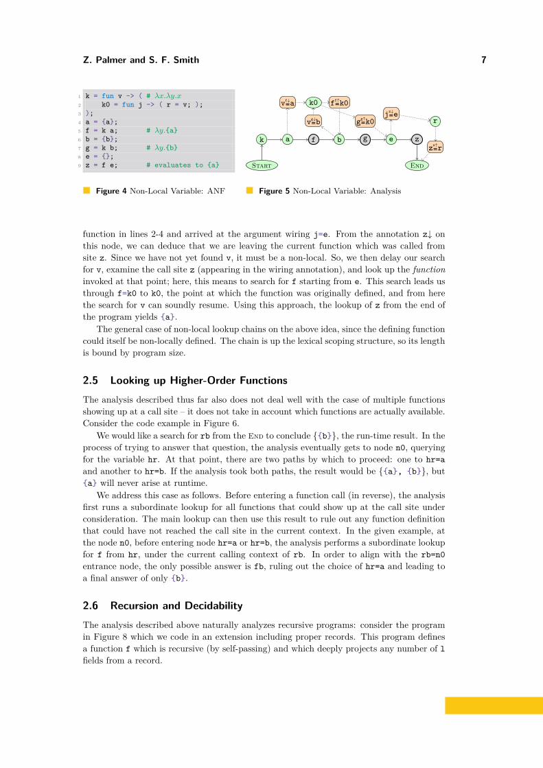
e ::= [c, . . .] abstract expressionsc ::= x = b abstract clausesb ::= v | x | x x | abs. bodies

x ~ p ? f : fx ::= x abstract variablesv ::= r | f abstract valuesp ::= r abstract patternsf ::= fun x -> ( e ) abs. functionsr ::= r abstract records

V ::= {v, . . .} abstract value setsa ::= c | abs. annotated clauses

xc↓= x | x c↑

= x | Start | Endd ::= a << a abstract dependenciesD ::= {d, . . .} abs. dependency graphsX ::= [x, . . .] abs. var lookup stacks

Figure 10 Analysis Grammar

3 The Analysis Formally

In this section we formalize the analysis algorithm. The operational semantics is standardand so we postpone it and the soundness proof to Section 4.

The grammar constructs needed for the analysis appear in Figure 10. The items on theleft are just the hatted versions of the corresponding program syntax. As mentioned above,we require variables to be bound uniquely so that each program point is defined by exactlyone variable. Furthermore, we assume the expressions we analyze to be closed: a variable isnot used until after the clause in which it is bound.

Edges in a dependency graph D are dependencies d, are written a << a′ and mean clausea happens right before clause a′. New clause annotations c↓ / c↑ are used to mark the entryand exit points for functions/cases.

I Definition 3.1. We use the following notational sugar for graph dependencies:We write a1 << a2 << . . . << an to mean {a1 << a2, . . . , an−1 << an}.We write a′ << {a1, . . . , an} (resp. {a1, . . . , an} << a′) to denote {a′ << a1, . . . , a

′ << an}(resp. {a1 << a′, . . . , an << a′}).We write a <� a′ to mean a << a′ ∈ D for some graph D understood from context.We define abbreviations Preds(a) = {a′ | a′ <� a} and Succs(a) = {a′ | a <� a′}.

I Definition 3.2. Initial embedding Embed([c1, . . . , cn]) is the graph D given by Start <<c1 << . . . << cn << End, where each ci = ci.

This initial graph is just the linear sequence of clauses in the “main program”.

3.1 LookupAs was described in Section 2, the analysis will look back along << edges in the graph D tosearch for definitions of variables it needs. We now define this lookup function.

3.1.1 Context StacksThe definition of lookup proceeds with respect to a current context stack C. The contextstack is used to align calls and returns to rule out cases of looking up a variable based on anon-sensical call stack, and was described in Section 2.3.

The proof of decidability relies upon bounding the depth of the call stack. We first definea general call stack model for DDPA, and in Section 3.3 below we instantiate the generalmodel with a fixed k-depth call stack version notated kDDPA; this is a simple boundingstrategy and our model can in principle work with other strategies.

10 Higher-Order Demand-Driven Program Analysis

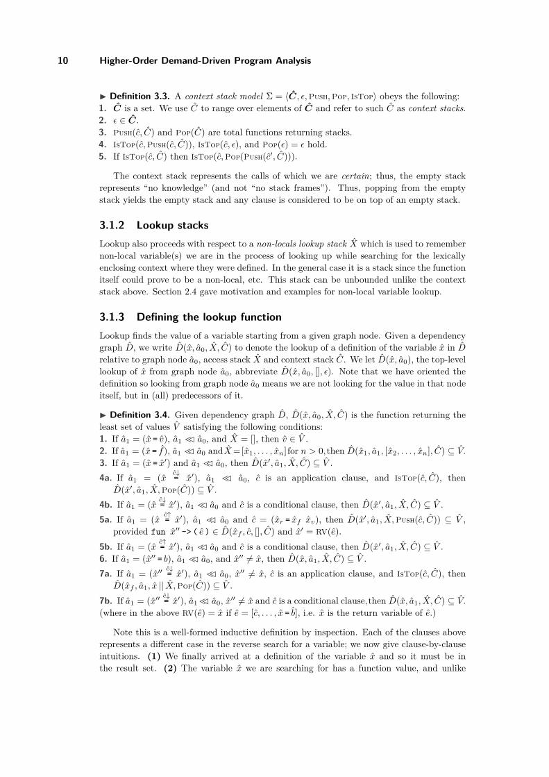
I Definition 3.3. A context stack model Σ = 〈C, ε,Push,Pop, IsTop〉 obeys the following:1. C is a set. We use C to range over elements of C and refer to such C as context stacks.2. ε ∈ C.3. Push(c, C) and Pop(C) are total functions returning stacks.4. IsTop(c,Push(c, C)), IsTop(c, ε), and Pop(ε) = ε hold.5. If IsTop(c, C) then IsTop(c,Pop(Push(c′, C))).

The context stack represents the calls of which we are certain; thus, the empty stackrepresents “no knowledge” (and not “no stack frames”). Thus, popping from the emptystack yields the empty stack and any clause is considered to be on top of an empty stack.

3.1.2 Lookup stacksLookup also proceeds with respect to a non-locals lookup stack X which is used to remembernon-local variable(s) we are in the process of looking up while searching for the lexicallyenclosing context where they were defined. In the general case it is a stack since the functionitself could prove to be a non-local, etc. This stack can be unbounded unlike the contextstack above. Section 2.4 gave motivation and examples for non-local variable lookup.

3.1.3 Defining the lookup functionLookup finds the value of a variable starting from a given graph node. Given a dependencygraph D, we write D(x, a0, X, C) to denote the lookup of a definition of the variable x in Drelative to graph node a0, access stack X and context stack C. We let D(x, a0), the top-levellookup of x from graph node a0, abbreviate D(x, a0, [], ε). Note that we have oriented thedefinition so looking from graph node a0 means we are not looking for the value in that nodeitself, but in (all) predecessors of it.

I Definition 3.4. Given dependency graph D, D(x, a0, X, C) is the function returning theleast set of values V satisfying the following conditions:1. If a1 = (x = v), a1 <� a0, and X = [], then v ∈ V .2. If a1 = (x = f), a1 <� a0 andX=[x1, . . . , xn]for n > 0, then D(x1, a1, [x2, . . . , xn], C) ⊆ V.3. If a1 = (x = x′) and a1 <� a0, then D(x′, a1, X, C) ⊆ V .4a. If a1 = (x c↓

= x′), a1 <� a0, c is an application clause, and IsTop(c, C), thenD(x′, a1, X,Pop(C)) ⊆ V .

4b. If a1 = (x c↓= x′), a1 <� a0 and c is a conditional clause, then D(x′, a1, X, C) ⊆ V .

5a. If a1 = (x c↑= x′), a1 <� a0 and c = (xr = xf xv), then D(x′, a1, X,Push(c, C)) ⊆ V ,

provided fun x′′ -> ( e ) ∈ D(xf , c, [], C) and x′ = RV(e).5b. If a1 = (x c↑

= x′), a1 <� a0 and c is a conditional clause, then D(x′, a1, X, C) ⊆ V .6. If a1 = (x′′ = b), a1 <� a0, and x′′ 6= x, then D(x, a1, X, C) ⊆ V .7a. If a1 = (x′′ c↓

= x′), a1 <� a0, x′′ 6= x, c is an application clause, and IsTop(c, C), thenD(xf , a1, x || X,Pop(C)) ⊆ V .

7b. If a1 = (x′′ c↓= x′), a1<� a0, x′′ 6= x and c is a conditional clause,then D(x, a1, X, C) ⊆ V.

(where in the above RV(e) = x if e = [c, . . . , x = b], i.e. x is the return variable of e.)

Note this is a well-formed inductive definition by inspection. Each of the clauses aboverepresents a different case in the reverse search for a variable; we now give clause-by-clauseintuitions. (1) We finally arrived at a definition of the variable x and so it must be inthe result set. (2) The variable x we are searching for has a function value, and unlike

Z. Palmer and S. F. Smith 11

clause (1) there is a non-empty lookup stack. This means the variable on top of the lookupstack, x1, was a non-local and was pushed on to the non-local stack while searching for thedefinition of the function it resides in. That function definition, x = f , has now been found,and so we may continue to search for x1 from the current point in the graph. (3) We havefound a definition of x but it is defined to be another variable x′. We transitively switchto looking for x′. (4a) We have reached the start of the function body and the variablex we are searching for was the formal argument x′. So, continue by searching for x′ fromthe call site. The IsTop clause constrains this stack frame exit to align with the frame wehad last entered (in reverse). (4b) This is the case clause version of the previous. Caseclauses can be viewed as inlined functions aligned by program context so use of C is notnecessary for alignment. (5a) We have reached a return copy which is assigning our variablex, so to look for x we need to continue by looking for x′ inside this function. Push c onthe stack since we are now entering the body (in reverse) via that call site. For a moreaccurate analysis, the “provided” line additionally requires that we only “walk back” intofunction(s) that could have reached this call site; so, we launch a subordinate lookup of xf

and constrain a1 accordingly. (6) Here the previous clause is not a match so the searchcontinues at any predecessor node. Note this will chain past function/match call sites whichdid not return the variable x we are looking for. This is sound in a pure functional language;when we address state in Section 5.3, we will enter such a function to verify an alias to ourvariable was not assigned. (7a) The precondition means we have reached the beginning ofa function body and did not find a definition for the variable x. In this case, we switch tosearching for the clause that defined the function body we are exiting, which is xf , and pushx on the non-locals stack. Once the defining point of xf is found, x will be popped fromthe non-locals stack and we will resume searching for it. The IsTop clause constrains thestack frame being exited to align with the frame we had last entered (in reverse). (7b) Thisis the case clause variation of the previous; as with (4b) above, the stack is not needed forconditional alignment – there is syntactically only one entry and exit.

3.2 Abstract EvaluationWe are now ready to present the single-step abstract evaluation relation on dependencygraphs. Like [28, 10] etc, it is a graph-based notion of evaluation, but where function bodiesare never copied – a single body is shared.

3.2.1 Active nodesIn order to preserve standard evaluation order we define the notion of an active node, Active– only nodes with all previous nodes already executed can fire. This serves a purpose similarto an evaluation context in operational semantics [4].

I Definition 3.5. Active(a′, D) iff path Start << a1 << . . . << an << a′ appears in D suchthat no ai is of one of the forms x = x′ x′′ or x = x′ ~ p ? f : f ′. We write Active(a′) when Dis understood from context.

3.2.2 WiringRecall from Section 2 how function application required the concrete function body to be“wired” directly in to the call site node, and how additional nodes were added to copy inthe argument and out the result. The following definition accomplishes this.

12 Higher-Order Demand-Driven Program Analysis

Applicationc = (x1 = x2 x3) Active(c, D) f ∈ D(x2, c) v ∈ D(x3, c)

D −→1 D ∪Wire(c, f, x3, x1)

Record Conditional Truec = (x1 = x2 ~ r ? f1 : f2) Active(c, D) r′ ∈ D(x2, c) r ⊆ r′

D −→1 D ∪Wire(c, f1, x2, x1)

Record Conditional Falsec = (x1 = x2 ~ r ? f1 : f2) Active(c, D) v ∈ D(x2, c) v of form r′ only if r * r′

D −→1 D ∪Wire(c, f2, x2, x1)

Figure 11 Abstract Evaluation Rules

I Definition 3.6. Let Wire(c′, fun x0 -> ( [c1, . . . , cn] ) , x1, x2) =Preds(c′) << (x0

c′↓= x1) << c1 << . . . << cn << (x2

c′↑= RV([cn])) << Succs(c′).

c′ here is the call site, and c1 << . . . << cn is the wiring of the function body. ThePreds/Succs functions (given above in Definition 3.1) reflect how we simply wire to theexisting predecessor(s) and successor(s).

Next, we define the abstract small-step relation −→1 on graphs, see Figure 11.

I Definition 3.7. We define the small step relation −→1 to hold if a proof exists in thesystem in Figure 11. We write D0 −→∗ Dn to denote D0 −→1 D1 −→1 . . . −→1 Dn.

The evaluation rules are straightforward after the above preliminaries. For application,if c is a call site that is an active redex, lookup of the function variable x2 returns functionbody f and some value v can be looked up at the argument position, we may wire in f ’sbody to this call site. Note that v is not added to the graph, it is only observed here toconstrain evaluation order to be call-by-value. The case clause rules are similar.

3.3 DecidabilityWe begin with the computability of the variable lookup operation, the source of all of thecomputational complexity of the analysis.

I Lemma 3.8. For any context stack model Σ with a finite C and computable Push/Pop/IsTopoperations, D(x0, a) is a computable function.

Proof. This proof proceeds by reduction to the problem of reachability in a push-downsystem (PDS) accepting by empty stack. A push-down system is a push-down automaton(PDA) with an empty input alphabet; PDA/PDS reachability is polynomial-time [3, 1].

We define a PDS in which each state is a pair between a program point and a contextstack (of which there are finitely many); the initial state is the pair a × ε. The stack ofthe PDS corresponds roughly to the lookup stack and the current variable of the lookupoperation: each variable of the source program is a member of the stack alphabet and theinitial PDS stack is then [x0] for computing D(x0, a). Each clause in Definition 3.4 (exceptclause 5a, which is discussed below) directly corresponds to a collection of transitions in thePDS. For instance, suppose a1 = (x′ = v′) and a1 << a0; then, by clauses 1 and 2, each nodea0 × C in the PDS transitions to a1 × C by popping x′ (and pushing no symbols).

Z. Palmer and S. F. Smith 13

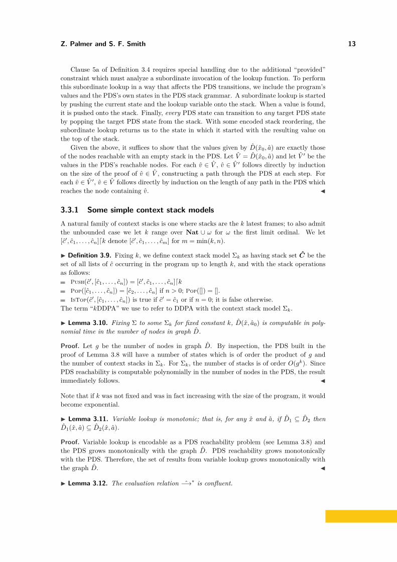
Clause 5a of Definition 3.4 requires special handling due to the additional “provided”constraint which must analyze a subordinate invocation of the lookup function. To performthis subordinate lookup in a way that affects the PDS transitions, we include the program’svalues and the PDS’s own states in the PDS stack grammar. A subordinate lookup is startedby pushing the current state and the lookup variable onto the stack. When a value is found,it is pushed onto the stack. Finally, every PDS state can transition to any target PDS stateby popping the target PDS state from the stack. With some encoded stack reordering, thesubordinate lookup returns us to the state in which it started with the resulting value onthe top of the stack.

Given the above, it suffices to show that the values given by D(x0, a) are exactly thoseof the nodes reachable with an empty stack in the PDS. Let V = D(x0, a) and let V ′ be thevalues in the PDS’s reachable nodes. For each v ∈ V , v ∈ V ′ follows directly by inductionon the size of the proof of v ∈ V , constructing a path through the PDS at each step. Foreach v ∈ V ′, v ∈ V follows directly by induction on the length of any path in the PDS whichreaches the node containing v. J

3.3.1 Some simple context stack modelsA natural family of context stacks is one where stacks are the k latest frames; to also admitthe unbounded case we let k range over Nat ∪ ω for ω the first limit ordinal. We let[c′, c1, . . . , cn]dk denote [c′, c1, . . . , cm] for m = min(k, n).

I Definition 3.9. Fixing k, we define context stack model Σk as having stack set C be theset of all lists of c occurring in the program up to length k, and with the stack operationsas follows:

Push(c′, [c1, . . . , cn]) = [c′, c1, . . . , cn]dkPop([c1, . . . , cn]) = [c2, . . . , cn] if n > 0; Pop([]) = [].IsTop(c′, [c1, . . . , cn]) is true if c′ = c1 or if n = 0; it is false otherwise.

The term “kDDPA” we use to refer to DDPA with the context stack model Σk.

I Lemma 3.10. Fixing Σ to some Σk for fixed constant k, D(x, a0) is computable in poly-nomial time in the number of nodes in graph D.

Proof. Let g be the number of nodes in graph D. By inspection, the PDS built in theproof of Lemma 3.8 will have a number of states which is of order the product of g andthe number of context stacks in Σk. For Σk, the number of stacks is of order O(gk). SincePDS reachability is computable polynomially in the number of nodes in the PDS, the resultimmediately follows. J

Note that if k was not fixed and was in fact increasing with the size of the program, it wouldbecome exponential.

I Lemma 3.11. Variable lookup is monotonic; that is, for any x and a, if D1 ⊆ D2 thenD1(x, a) ⊆ D2(x, a).

Proof. Variable lookup is encodable as a PDS reachability problem (see Lemma 3.8) andthe PDS grows monotonically with the graph D. PDS reachability grows monotonicallywith the PDS. Therefore, the set of results from variable lookup grows monotonically withthe graph D. J

I Lemma 3.12. The evaluation relation −→∗ is confluent.

14 Higher-Order Demand-Driven Program Analysis

Proof. By inspection of Figure 11, the single-step rules only add to graph D. The Activerelation is also clearly monotone: any enabled redex is never disabled. Confluence is trivialfrom these two facts. J

I Lemma 3.13. The evaluation relation −→∗ is terminating, i.e. for any D0 there exists aDn such that D0 −→∗ Dn and if Dn −→∗ Dn+1, Dn = Dn+1. Furthermore, n is polynomialin the size of the initial program.

Proof. By inspection of Figure 11, we have for any step D′ −→1 D′′ that D′ ⊆ D′′. Theonly new nodes that can be added to D in the course of evaluation are the entry/exit nodesx′

c↓= x / x c↑

= x′, and only one of each of those nodes can exist for each call site (or caseclause) / function body pair in the source program: c is the call site, and x / x′ are variablesin that call site and function body source, respectively. So, the number of nodes that can beadded is always less then two times the square of the size of the original program. A similarargument holds for added edges. J

We let D ↓ D′ abbreviate D −→∗ D′ such that D′ −→1 D′. We write e ↓ D to abbreviateEmbed(e) ↓ D; this means the analysis of e returns graph D. Given the pieces assembledabove, it is now easy to prove that the analysis is polynomial-time.

I Theorem 3.14. Fixing Σ to be some Σk and fixing some expression e, the analysis resultD, where e ↓ D, is computable in time polynomial in the size of e.

Proof. By Lemma 3.10, each lookup operation takes poly-time. The evaluation rules aretrivial computations besides the required lookups and, by Lemma 3.13, there are polynomi-ally many evaluation steps before termination. Thus e ↓ D is computable in poly-time. J

4 Soundness

We now establish soundness of the analysis defined in the previous section. In forwardprogram analyses the alignment between the operational semantics and analysis is fairlyclose and so soundness is not particularly difficult, but here there is a larger gap. Wecross this river by throwing a stone in the middle: along with defining a mostly-standardoperational semantics we build a graph-based operational semantics which creates a concretecall graph of the program run that is more directly aligned with the analysis. Soundness isthen shown by proving the standard and graph-based operational semantics equivalent andby showing the analysis sound with respect to the graph-based operational semantics.

In this section we first present the standard operational semantics, then the graph-based operational semantics and its equivalence to the standard one, and finally we provesoundness.

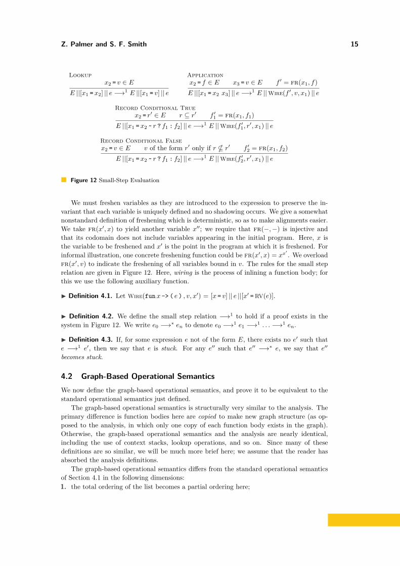
4.1 Standard Operational SemanticsThe operational semantics appears in Figure 12, as a small step relation e −→1 e′. In manyways the operational semantics is standard, but due to our use of an A-normal form it isneither precisely substitution-based nor environment-based. It is more substitution-basedin spirit since function bodies are inlined. Although variable lookup is via an environment,all names in that environment are deterministically freshened and so no variable shadowingever arises; so, although variable lookup might appear to be dynamically scoped, the absenceof shadowing ensures static scoping. This model of evaluation is designed to integrate wellwith the graph-based semantics of the next sub-section.

Z. Palmer and S. F. Smith 15

Lookupx2 = v ∈ E

E ||[x1 =x2] || e −→1 E ||[x1 = v] || e

Applicationx2 = f ∈ E x3 = v ∈ E f ′ = fr(x1, f)E ||[x1 =x2 x3] || e −→1 E ||Wire(f ′, v, x1) || e

Record Conditional Truex2 = r′ ∈ E r ⊆ r′ f ′1 = fr(x1, f1)

E ||[x1 =x2 ~ r ? f1 : f2] || e −→1 E ||Wire(f ′1, r′, x1) || e

Record Conditional Falsex2 = v ∈ E v of the form r′ only if r * r′ f ′2 = fr(x1, f2)

E ||[x1 =x2 ~ r ? f1 : f2] || e −→1 E ||Wire(f ′2, r′, x1) || e

Figure 12 Small-Step Evaluation

We must freshen variables as they are introduced to the expression to preserve the in-variant that each variable is uniquely defined and no shadowing occurs. We give a somewhatnonstandard definition of freshening which is deterministic, so as to make alignments easier.We take fr(x′, x) to yield another variable x′′; we require that fr(−,−) is injective andthat its codomain does not include variables appearing in the initial program. Here, x isthe variable to be freshened and x′ is the point in the program at which it is freshened. Forinformal illustration, one concrete freshening function could be fr(x′, x) = xx′ . We overloadfr(x′, v) to indicate the freshening of all variables bound in v. The rules for the small steprelation are given in Figure 12. Here, wiring is the process of inlining a function body; forthis we use the following auxiliary function.

I Definition 4.1. Let Wire(funx -> ( e ) , v, x′) = [x = v] || e ||[x′ = RV(e)].

I Definition 4.2. We define the small step relation −→1 to hold if a proof exists in thesystem in Figure 12. We write e0 −→∗ en to denote e0 −→1 e1 −→1 . . . −→1 en.

I Definition 4.3. If, for some expression e not of the form E, there exists no e′ such thate −→1 e′, then we say that e is stuck. For any e′′ such that e′′ −→∗ e, we say that e′′becomes stuck.

4.2 Graph-Based Operational SemanticsWe now define the graph-based operational semantics, and prove it to be equivalent to thestandard operational semantics just defined.

The graph-based operational semantics is structurally very similar to the analysis. Theprimary difference is function bodies here are copied to make new graph structure (as op-posed to the analysis, in which only one copy of each function body exists in the graph).Otherwise, the graph-based operational semantics and the analysis are nearly identical,including the use of context stacks, lookup operations, and so on. Since many of thesedefinitions are so similar, we will be much more brief here; we assume that the reader hasabsorbed the analysis definitions.

The graph-based operational semantics differs from the standard operational semanticsof Section 4.1 in the following dimensions:1. the total ordering of the list becomes a partial ordering here;

16 Higher-Order Demand-Driven Program Analysis

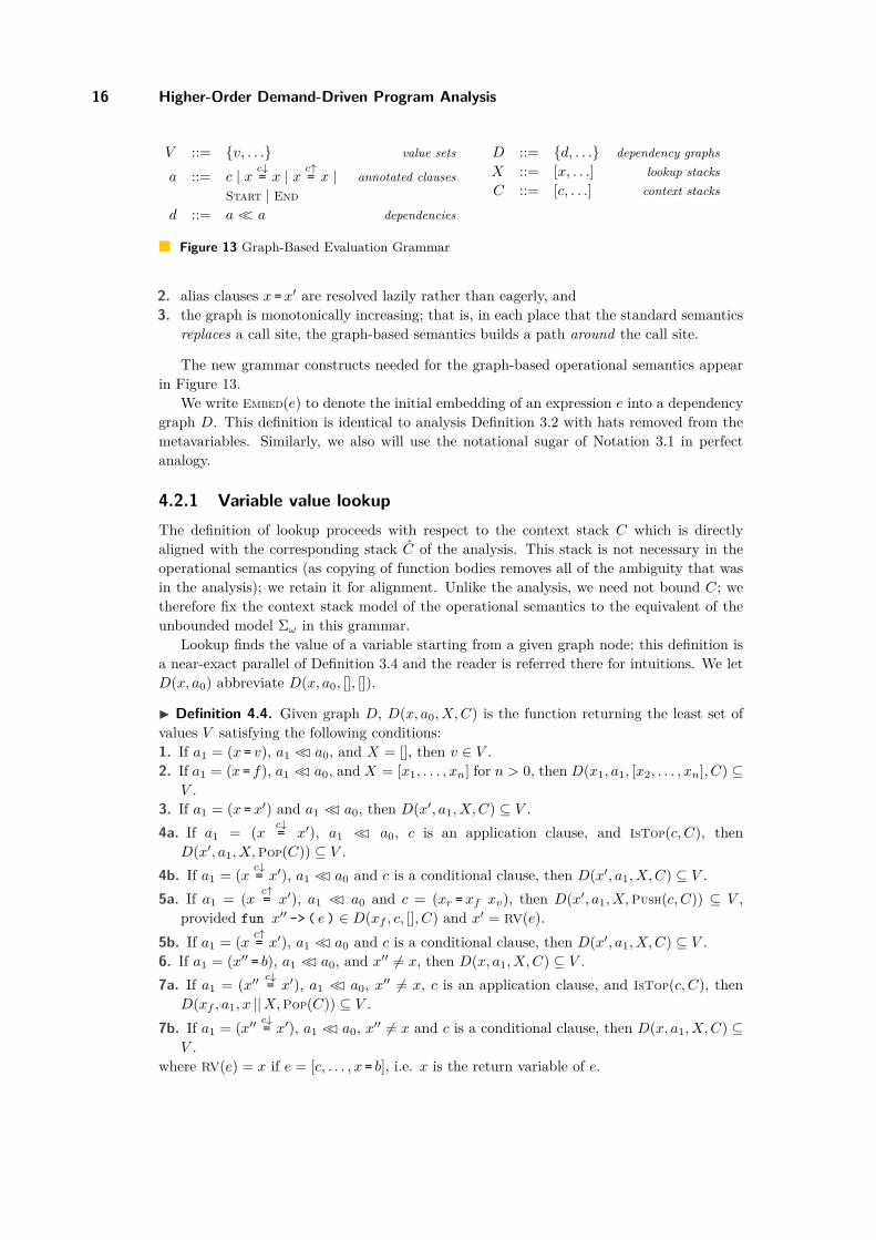
V ::= {v, . . .} value sets

a ::= c | x c↓= x | x c↑

= x | annotated clausesStart | End

d ::= a << a dependencies

D ::= {d, . . .} dependency graphsX ::= [x, . . .] lookup stacksC ::= [c, . . .] context stacks

Figure 13 Graph-Based Evaluation Grammar

2. alias clauses x =x′ are resolved lazily rather than eagerly, and3. the graph is monotonically increasing; that is, in each place that the standard semantics

replaces a call site, the graph-based semantics builds a path around the call site.

The new grammar constructs needed for the graph-based operational semantics appearin Figure 13.

We write Embed(e) to denote the initial embedding of an expression e into a dependencygraph D. This definition is identical to analysis Definition 3.2 with hats removed from themetavariables. Similarly, we also will use the notational sugar of Notation 3.1 in perfectanalogy.

4.2.1 Variable value lookupThe definition of lookup proceeds with respect to the context stack C which is directlyaligned with the corresponding stack C of the analysis. This stack is not necessary in theoperational semantics (as copying of function bodies removes all of the ambiguity that wasin the analysis); we retain it for alignment. Unlike the analysis, we need not bound C; wetherefore fix the context stack model of the operational semantics to the equivalent of theunbounded model Σω in this grammar.

Lookup finds the value of a variable starting from a given graph node; this definition isa near-exact parallel of Definition 3.4 and the reader is referred there for intuitions. We letD(x, a0) abbreviate D(x, a0, [], []).

I Definition 4.4. Given graph D, D(x, a0, X,C) is the function returning the least set ofvalues V satisfying the following conditions:1. If a1 = (x = v), a1 <� a0, and X = [], then v ∈ V .2. If a1 = (x = f), a1 <� a0, and X = [x1, . . . , xn] for n > 0, then D(x1, a1, [x2, . . . , xn], C) ⊆

V .3. If a1 = (x =x′) and a1 <� a0, then D(x′, a1, X,C) ⊆ V .4a. If a1 = (x c↓

= x′), a1 <� a0, c is an application clause, and IsTop(c, C), thenD(x′, a1, X,Pop(C)) ⊆ V .

4b. If a1 = (x c↓= x′), a1 <� a0 and c is a conditional clause, then D(x′, a1, X,C) ⊆ V .

5a. If a1 = (x c↑= x′), a1 <� a0 and c = (xr =xf xv), then D(x′, a1, X,Push(c, C)) ⊆ V ,

provided fun x′′ -> ( e ) ∈ D(xf , c, [], C) and x′ = RV(e).5b. If a1 = (x c↑

= x′), a1 <� a0 and c is a conditional clause, then D(x′, a1, X,C) ⊆ V .6. If a1 = (x′′ = b), a1 <� a0, and x′′ 6= x, then D(x, a1, X,C) ⊆ V .7a. If a1 = (x′′ c↓

= x′), a1 <� a0, x′′ 6= x, c is an application clause, and IsTop(c, C), thenD(xf , a1, x ||X,Pop(C)) ⊆ V .

7b. If a1 = (x′′ c↓= x′), a1 <� a0, x′′ 6= x and c is a conditional clause, then D(x, a1, X,C) ⊆

V .where RV(e) = x if e = [c, . . . , x = b], i.e. x is the return variable of e.

Z. Palmer and S. F. Smith 17

Applicationc = (x1 =x2 x3) Active(c,D) f ∈ D(x2, c) v ∈ D(x3, c) f ′ = fr(x1, f)

D −→1 D ∪Wire(c, f ′, x3, x1)

Record Conditional Truec = (x1 =x2 ~ r ? f1 : f2) Active(c,D) r′ ∈ D(x2, c) r ⊆ r′ f ′1 = fr(x1, f1)

D −→1 D ∪Wire(c, f ′1, x2, x1)

Record Conditional Falsec = (x1 =x2 ~ r ? f1 : f2)

Active(c,D) v ∈ D(x2, c) v of form r′ only if r * r′ f ′2 = fr(x1, f2)D −→1 D ∪Wire(c, f ′2, x2, x1)

Figure 14 Graph Evaluation Rules

4.2.2 The evaluation relationThe definition of an active node, Active, exactly parallels the analysis version of Definition3.5, simply remove the hats from the metavariables. We write Active(a′) when D is un-derstood from context. Wiring is also defined in perfect analogy with Definition 3.6 so isomitted here. The small-step relation −→1 on graphs is defined in Figure 14. (Note weoverload symbol −→1 for the list and graph operational semantics, it is clear from contextwhich relation is intended.)

I Definition 4.5. We define the small step relation −→1 to hold if a proof exists in thesystem in Figure 14. We write D0 −→∗ Dn to denote D0 −→1 D1 −→1 . . . −→1 Dn.

We also define a notion of “stuckness” for graphs in parallel with the standard operationalsemantics.

These rules are very similar to the analysis transition rules in Section 3.2; we refer thereader to the descriptions there. Here we comment on a few points unique to the operationalsemantics not found in the analysis.

We are precise about freshening in these rules. Because the fr(x,−) function is deter-ministically freshening based on the call site x, it will always generate the same result for thesame call site and value. This means that e.g. each use of the Application rule is idempotentand the graph-based operational semantics is deterministic.

Observe how Figure 14 is defining a “reduction” relation which is in fact monotonicallyincreasing, an unusual property compared to standard operational semantics.

4.3 Proving Equivalence of Operational SemanticsThe overall proof of soundness relies upon showing that these two systems of operationalsemantics are equivalent. To demonstrate this, we must show several properties of thegraph-based operational semantics which are less obvious than in the standard operationalsemantics due to the structure of the graph. As stated above, the real differences betweenthese systems are (1) the partial ordering of clauses, (2) lazy resolution of alias clauses, and(3) that the graph grows monotonically instead of replacing applications and conditionals.Nonetheless, the graph representation “runs” in the same way that expressions do: there isa unique clause which is evaluated next, it may cause the introduction of more clauses, and

18 Higher-Order Demand-Driven Program Analysis

complex clauses (applications and conditionals) are handled by wiring and evaluating theappropriate function body.

We use this reasoning to establish a bisimulation ∼= between an expression and its em-bedding and then show that this bisimulation is preserved as evaluation proceeds. Thebisimulation and corresponding preservation proof are tedious and intuitive, so we excludethem for reasons of space. The key equivalence lemma is stated as follows.

I Lemma 4.6 (Equivalence of standard and graph-based semantics). If e ∼= D, then1. If e −→1 e′ then D −→∗ D′ such that e′ ∼= D′.2. If D −→1 D′ then e −→∗ e′ such that e′ ∼= D′.

This equivalence is one-to-many to accommodate the differences between the two oper-ational semantics relations. The graph opsems lazily resolves aliases, meaning that severalsteps of the standard opsems may be required to propagate a value that the graph wouldfind via lookup (Definition 4.4). Likewise, a single lookup step of the standard opsems mayrequire no changes to the graph to maintain bisimulation.

4.4 Soundness of the Analysis

We now show that the analysis simulates the graph-based operational semantics, D 4 D.This proof is easy, as the operational semantics graph can be projected on to an analysisgraph by inverting the variable freshening function. We formally define this inversion asfollows:

I Definition 4.7. The origin of a variable x is x itself if x is not in the codomain offr(−,−). Otherwise, let fr(x′′, x′) = x (for unique x′′ and x′, as fr(−,−) is injective).Then the origin of x is the origin of x′.

We next define the simulation between evaluation graphs and analysis graphs. The graphoperational semantics was designed explicitly to make this simulation direct.

IDefinition 4.8 (Simulation relation). Let f be the natural graph-and-clause homomorphismfrom an evaluation graph D to an analysis graph D which maps variables to their origins.We say that D is simulated by D (written D 4 D) iff f(D) = D.

I Lemma 4.9 (Soundness). If D 4 D and D −→1 D′, then D −→1 D′ with D′ 4 D′.

Proof. By case analysis on the rule used to prove D −→1 D′. In particular, the premisesof a corresponding rule D −→1 D′ can be proven using the premises of D −→1 D′ and thesimulation. J

5 Extensions

In this section, we outline three extensions: full records, path sensitivity, and mutable state.Our goal here is to show there is no fundamental limitation to the model given in theprevious sections: DDPA can in principle be extended to the full feature set of a realisticprogramming language. Here for simplicity of presentation we take each feature one at atime; in a language where they are all simultaneously added there are additional featureinteraction cases that must be addressed.

Z. Palmer and S. F. Smith 19

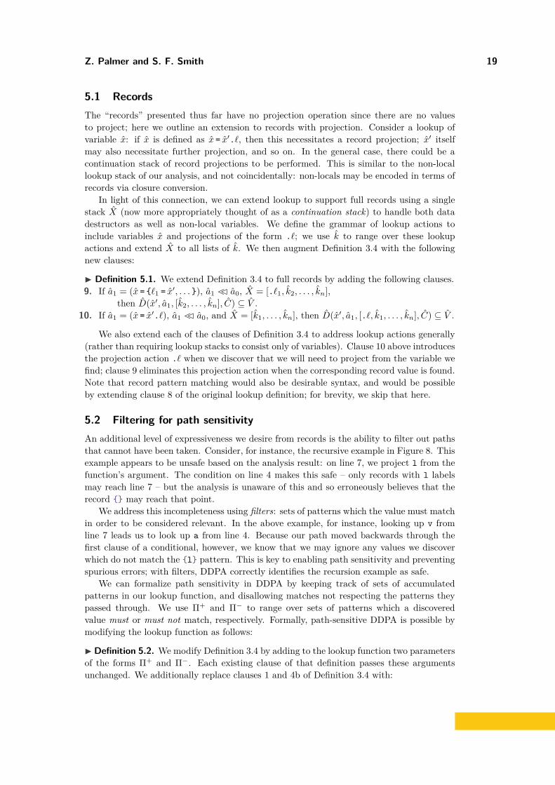
5.1 RecordsThe “records” presented thus far have no projection operation since there are no valuesto project; here we outline an extension to records with projection. Consider a lookup ofvariable x: if x is defined as x = x′.`, then this necessitates a record projection; x′ itselfmay also necessitate further projection, and so on. In the general case, there could be acontinuation stack of record projections to be performed. This is similar to the non-locallookup stack of our analysis, and not coincidentally: non-locals may be encoded in terms ofrecords via closure conversion.

In light of this connection, we can extend lookup to support full records using a singlestack X (now more appropriately thought of as a continuation stack) to handle both datadestructors as well as non-local variables. We define the grammar of lookup actions toinclude variables x and projections of the form .`; we use k to range over these lookupactions and extend X to all lists of k. We then augment Definition 3.4 with the followingnew clauses:

I Definition 5.1. We extend Definition 3.4 to full records by adding the following clauses.9. If a1 = (x = {`1 = x′, . . . }), a1 <� a0, X = [.`1, k2, . . . , kn],

then D(x′, a1, [k2, . . . , kn], C) ⊆ V .10. If a1 = (x = x′.`), a1 <� a0, and X = [k1, . . . , kn], then D(x′, a1, [.`, k1, . . . , kn], C) ⊆ V .

We also extend each of the clauses of Definition 3.4 to address lookup actions generally(rather than requiring lookup stacks to consist only of variables). Clause 10 above introducesthe projection action .` when we discover that we will need to project from the variable wefind; clause 9 eliminates this projection action when the corresponding record value is found.Note that record pattern matching would also be desirable syntax, and would be possibleby extending clause 8 of the original lookup definition; for brevity, we skip that here.

5.2 Filtering for path sensitivityAn additional level of expressiveness we desire from records is the ability to filter out pathsthat cannot have been taken. Consider, for instance, the recursive example in Figure 8. Thisexample appears to be unsafe based on the analysis result: on line 7, we project l from thefunction’s argument. The condition on line 4 makes this safe – only records with l labelsmay reach line 7 – but the analysis is unaware of this and so erroneously believes that therecord {} may reach that point.

We address this incompleteness using filters: sets of patterns which the value must matchin order to be considered relevant. In the above example, for instance, looking up v fromline 7 leads us to look up a from line 4. Because our path moved backwards through thefirst clause of a conditional, however, we know that we may ignore any values we discoverwhich do not match the {l} pattern. This is key to enabling path sensitivity and preventingspurious errors; with filters, DDPA correctly identifies the recursion example as safe.

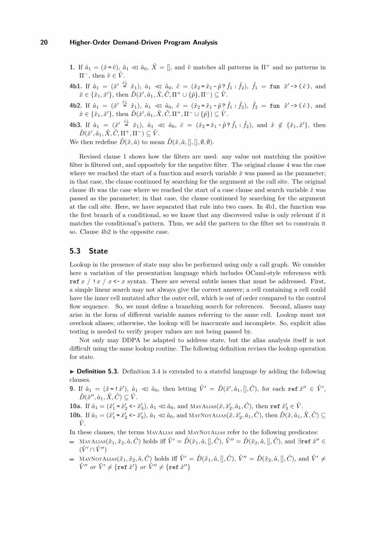
We can formalize path sensitivity in DDPA by keeping track of sets of accumulatedpatterns in our lookup function, and disallowing matches not respecting the patterns theypassed through. We use Π+ and Π− to range over sets of patterns which a discoveredvalue must or must not match, respectively. Formally, path-sensitive DDPA is possible bymodifying the lookup function as follows:

I Definition 5.2. We modify Definition 3.4 by adding to the lookup function two parametersof the forms Π+ and Π−. Each existing clause of that definition passes these argumentsunchanged. We additionally replace clauses 1 and 4b of Definition 3.4 with:

20 Higher-Order Demand-Driven Program Analysis

1. If a1 = (x = v), a1 <� a0, X = [], and v matches all patterns in Π+ and no patterns inΠ−, then v ∈ V .

4b1. If a1 = (x′ c↓= x1), a1 <� a0, c = (x2 = x1 ~ p ? f1 : f2), f1 = fun x′ -> ( e ), and

x ∈ {x1, x′}, then D(x′, a1, X, C,Π+ ∪ {p},Π−) ⊆ V .

4b2. If a1 = (x′ c↓= x1), a1 <� a0, c = (x2 = x1 ~ p ? f1 : f2), f2 = fun x′ -> ( e ), and

x ∈ {x1, x′}, then D(x′, a1, X, C,Π+,Π− ∪ {p}) ⊆ V .

4b3. If a1 = (x′ c↓= x1), a1 <� a0, c = (x2 = x1 ~ p ? f1 : f2), and x /∈ {x1, x

′}, thenD(x′, a1, X, C,Π+,Π−) ⊆ V .

We then redefine D(x, a) to mean D(x, a, [], [], ∅, ∅).

Revised clause 1 shows how the filters are used: any value not matching the positivefilter is filtered out, and oppositely for the negative filter. The original clause 4 was the casewhere we reached the start of a function and search variable x was passed as the parameter;in that case, the clause continued by searching for the argument at the call site. The originalclause 4b was the case where we reached the start of a case clause and search variable x waspassed as the parameter; in that case, the clause continued by searching for the argumentat the call site. Here, we have separated that rule into two cases. In 4b1, the function wasthe first branch of a conditional, so we know that any discovered value is only relevant if itmatches the conditional’s pattern. Thus, we add the pattern to the filter set to constrain itso. Clause 4b2 is the opposite case.

5.3 StateLookup in the presence of state may also be performed using only a call graph. We considerhere a variation of the presentation language which includes OCaml-style references withref x / !x / x <- x syntax. There are several subtle issues that must be addressed. First,a simple linear search may not always give the correct answer; a cell containing a cell couldhave the inner cell mutated after the outer cell, which is out of order compared to the controlflow sequence. So, we must define a branching search for references. Second, aliases mayarise in the form of different variable names referring to the same cell. Lookup must notoverlook aliases; otherwise, the lookup will be inaccurate and incomplete. So, explicit aliastesting is needed to verify proper values are not being passed by.

Not only may DDPA be adapted to address state, but the alias analysis itself is notdifficult using the same lookup routine. The following definition revises the lookup operationfor state.

I Definition 5.3. Definition 3.4 is extended to a stateful language by adding the followingclauses.9. If a1 = (x = ! x′), a1 <� a0, then letting V ′ = D(x′, a1, [], C), for each ref x′′ ∈ V ′,

D(x′′, a1, X, C) ⊆ V .10a. If a1 = (x′1 = x′2 <- x′3), a1 <� a0, and MayAlias(x, x′2, a1, C), then ref x′3 ∈ V .10b. If a1 = (x′1 = x′2 <- x′3), a1 <� a0, and MayNotAlias(x, x′2, a1, C), then D(x, a1, X, C) ⊆

V .In these clauses, the terms MayAlias and MayNotAlias refer to the following predicates:

MayAlias(x1, x2, a, C) holds iff V ′ = D(x1, a, [], C), V ′′ = D(x2, a, [], C), and ∃ref x′′ ∈(V ′ ∩ V ′′)MayNotAlias(x1, x2, a, C) holds iff V ′ = D(x1, a, [], C), V ′′ = D(x2, a, [], C), and V ′ 6=V ′′ or V ′ 6= {ref x′} or V ′′ 6= {ref x′′}

Z. Palmer and S. F. Smith 21

Clause 9 handles dereferencing. It finds the ref values which may be in x′ at this pointin the program; it then returns to this point to find all of the values that those variables maycontain. This new task is necessary since we want the value at the point the ! happened.

Clauses 10a and 10b address cell updates. Clause 10a determines if the updated cell in x′2may alias the cell we are looking up; if this is the case, the value assigned by the cell updatemay be our answer. Clause 10b addresses the case in which the updated cell may be differentfrom the target of our lookup. This happens when the lookups of each variable yield differentresults or when they result in multiple cells – even if the sets of cells are equal, the ordersin which the program modifies the cells might differ, so we take the conservative approachand call them different. MayAlias and MayNotAlias can be simultaneously satisfiable; whenthat happens, the analysis explores both clauses 10a and 10b.

Along with the above modifications, the existing clauses 5 and 6 need to be extended tosupport state. As written, clause 6 allows us to skip by call sites and pattern matches whoseoutput do not match the variable for which we are searching. This is sound in a pure system,but in the presence of side-effects we must explore these clauses to ensure that they did notaffect the cell we are attempting to dereference. We thus modify clause 6 by prohibiting bfrom being a call site or pattern match. We require a new clause similar to clause 5 but forthe case in which the search variable does not match the output variable. In that case, weproceed into the body of the function but in a “side-effect only” mode: we skip by everyclause which is not a cell assignment or does not lead to one. We leave side-effect only modeonce we leave the beginning of the function which initiated it.

6 Implementation

We have developed a proof-of-concept implementation of DDPA [17]; a copy of the imple-mentation is archived as an artifact with this paper. This implementation analyzes thepresentation language given in Section 2 extended to the proper record semantics describedin Section 5. The implementation correctly generates all control-flow graphs and valuelookup results given in the overview.

Although the proof-of-concept implementation demonstrates the behavior of DDPA, itis far from efficient and we are presently developing a performant implementation. Our im-plementation follows the lookup algorithm outlined in the proof of Lemma 3.8: we constructa push-down automaton modeling a non-deterministic backwards walk of the DDPA graphand then analyze this PDA for states reachable with an empty stack. There is a wealth ofliterature on PDA reachability algorithms [3, 1] which we can utilize to gain efficiency; inparticular, [3] includes an algorithm for eliminating spurious nodes and edges which we havealready integrated into the proof-of-concept implementation due to its simplicity.

7 Related Work

7.1 CFL-reachabilityThe core idea of our analysis can be viewed as extending first-order demand-driven CFL-reachability analyses [6] to the higher-order case: the analysis is centered around using aCFG, calls and returns are aligned, and lookup is computed lazily. Two issues make thehigher-order analysis challenging: the CFG needs to be computed on-the-fly due to thepresence of higher-order functions, and non-local variable lookup is subtle. The aforeciteddemand-driven analyses delve further into the trade-off between active propagation anddemand-driven lookup, and this is something we plan to explore in future work. There

22 Higher-Order Demand-Driven Program Analysis

are many other first-order program analyses with a demand-driven component; several useDatalog-style specification formats [19] including [29, 23].

Higher-order program analyses have been built which also incorporate call-return align-ment [26, 8], but these higher-order analyses are not demand-driven and have a differentalgorithmic basis. We now contrast DDPA with these and other higher-order program anal-yses.

7.2 Higher-order program analysisAs mentioned in the Introduction, higher-order program analyses today are generally con-structed by abstract interpretation [2], a finitization process on the operational seman-tics. We refer to these analyses as forward analyses to contrast with the backward-looking,demand-driven approach of DDPA.

In the most basic forward analysis, a new state is created for each new program point/s-tore/environment, and the number of states grows too rapidly to be practical. Modificationsincluding store widening, abstract garbage collection, polyvariance, and call-return align-ment are thus added as means to obtain a better trade-off of expressiveness vs size of statespace. DDPA in some sense comes from the opposite direction: the global state informationis a graph isomorphic to the CFG which is polynomial in size and will be smaller than thestate space of any forward analysis. However, variable lookup is of high complexity and weneed to “spend” more space to make it more efficient.

We will expand by considering the different dimensions of analysis expressiveness in turn.We begin with flow-sensitivity, meaning the analysis is sensitive to the order of assignmentoperations. Forward analyses are initially flow-sensitive since each abstract state has its ownstore, but the standard store widening optimization unifies these stores and eliminates flow-sensitivity. One alternative is abstract garbage collection [14, 8], which requires a per-nodestore (since, if the store were global, there would be no garbage). Abstract garbage preservesflow-sensitivity while reducing abstract states caused by local data, but state explosions stilloccur with persistent data. DDPA is flow-sensitive and garbage-free by construction: itis flow-sensitive because variables are looked up with respect to a program point, and itis garbage-free vacuously (as no stores are ever created). In a practical implementation ofDDPA, the caching of values will bring it closer to an abstract garbage collection approach,but abstract garbage collection is bottom-up as opposed to top-down: rather than deletingitems proved unneeded, items are added only if they may be needed in the future.

Another important dimension of expressiveness is polyvariance: whether functions cantake on different forms in different contexts of use. The classic higher-order polyvariancemodel is kCFA [22], which copies contours in analogy to forall-elimination in a polymorphictype system. But there are many routes to behavior that appears as polyvariance. With-out store widening, flow-sensitivity alone can distinguish calling context and provide somepolyvariance. Additionally, call-return alignment can provide different contexts for differ-ent function calls. The example we gave in Figure 3, for instance, needs only call-returnalignment to give polyvariant behavior in DDPA.

Call-return alignment was first explored in a higher-order context in subtype constrainttheories [18]; this work also uses the demand-driven nature of CFL-reachability to optimizelookup. However, it is flow-insensitive, uses let-polymorphism only, and does not align non-local variables, and so is not in the same category of analysis. In the context of abstractinterpretation, the first such algorithm was CFA2 [26], which was subsequently extendedand refined in kPDCFA [8]. We compare primarily with the more recent kPDCFA here.

An important observation of [8] regarding kPDCFA was that, in the presence of abstract

Z. Palmer and S. F. Smith 23

garbage collection, it is not possible to have an arbitrary stack for aligning calls and returns.That paper proposes a regular expression modeling of call stacks to make the analysiscomputable. We have a similar problem: our analysis finitizes one of its two stacks toconform to a PDA encoding. We define the family of analyses kDDPA (Definition 3.3)where k is the maximum stack depth for call-return alignments. Our finitization here issimpler than the regular expression approach of kPDCFA; the regular expression approachmay work in our context and is a topic for future investigation.

DDPA achieves greater polyvariance solely from call-return alignment when comparedwith kPDCFA or CFA2. In kPDCFA, stack alignment can be used to provide a differentcontext for function parameters, but non-local variables get no such advantage since theyare not in the local stack context. In DDPA, the stack context is still applicable to non-local variable lookup as shown in Figure 5. In fact, we conjecture that, for a program with amaximal lexical nesting depth of c, the analysis (k+c)DDPA will be at least as expressive askCFA (and should be more expressive due to alignment of calls and returns). The additionalc levels are needed because, in the worst case, each extra lexical level requires the lookupof a non-local variable and thus a position on the lookup stack. This way, DDPA achieveswith only stack alignment what forward analyses need both stack alignment and polyvariantcontours to accomplish.

The run-time complexity of kDDPA can also be framed in terms of the expressivenessof non-local variable polyvariance. It is shown in [15] how non-locals are the (only) sourceof exponential behavior in kCFA [24]; in particular, if lexical nesting were assumed to be ofsome constant depth not tied to the size of the program, kCFA would not be exponential.The complexity of kDDPA comes from the other direction: for any fixed k, the algorithmkDDPA is polynomial; but k needs to be increased by one for each level of stack alignmentwe wish to achieve in non-local lookup. For pathologically nested programs, k must be onthe order of the size of the program for kDDPA to avoid imprecision due to non-local lookup.Because kDDPA’s complexity is exponential in k, such a non-local-precise kDDPA wouldbe exponentially complex in that pathological case.

Related to this are provably polynomial context-sensitive analyses which, like kDDPA,restrict context-sensitivity in the case of high degree of lexical nesting [7, 15]. mCFA [15]is a polyvariant analysis hierarchy for functional languages that is provably polynomial incomplexity. This is achieved by an analysis that “in spirit” is working over closure-convertedsource programs: by factoring out all non-local variable references, the worst-case behaviorhas also been removed. Unfortunately, this also affects the precision of the analysis: non-locals that are distinguished in kCFA are merged inmCFA. In kDDPA, the level of non-localprecision is built into the constant k of how deep the run-time stack approximation is, somore precision is achieved as k increases. mCFA does not have this property: non-localswill always be monomorphised for any m.

Our current implementation is a proof-of-concept only; we plan to investigate ideasin [11, 8, 9] and other papers for more performant PDA reachability algorithms. Overallthe trade-offs in performance and expressiveness are subtle and implementations will benecessary to decide how practically useful DDPA is.

8 Conclusions

In this paper, we have developed a demand-driven program analysis (DDPA) for higher-orderprograms which is centered around production of a call graph. DDPA needs only the callgraph to look up variable values; the specification does not maintain any other structures.

24 Higher-Order Demand-Driven Program Analysis

DDPA can be viewed as the adaptation of previous CFL-reachability-based demand-drivenprogram analyses to higher-order programs. This adaptation required two key changes.First, it was necessary to incrementally construct the control-flow graph as the analysisproceeded; second, the lookup of non-local variables required special handling.

We believe DDPA shows promise primarily because it represents a significantly differentapproach compared with other higher-order analyses. A high-level analogy can be madewith eager and lazy programming languages: it is a fundamental decision in language designwhich approach to take and there are significant trade-offs. We believe the demand-drivenside of higher-order program analyses deserves further exploration.

We have established a polynomial-time bound on a higher-order program analysis whichis both flow- and context-sensitive. The reduced global state size holds out promise forprogram verification tools: the fewer the states, the less overwhelming the workload will befor a model checker, theorem prover, or other verification strategy.

We present preliminary results here from a simple implementation to serve as a confir-mation of correctness, but our implementation needs tuning and would benefit from a head-to-head comparison with some state-of-the-art analyses. Although DDPA’s value lookup isnovel, it shares the task of PDA reachability with the existing program analysis literatureand so a rich body of work is available to be utilized in implementing DDPA efficiently.

We believe the analysis should scale well to other language features, and have presentedoutlines for extensions of the basic analysis to deep data structures, path-sensitivity, andstate; we leave efficient decision procedures for the latter two to future work. We also intendto explore the development of extensions for other language features: exceptions and othercontrol operators, concurrency, and modularity to name a few.

Acknowledgements We thank Alex Rozenshteyn for motivating our interest in AAM [25]and related papers which then led to our formulation of DDPA.We thank David Van Horn fordiscussions helping us better understand the AAM work. We also thank Leandro Facchinettifor his detailed review of this paper and his contributions to the accompanying artifact.

References1 Ahmed Bouajjani, Javier Esparza, and Oded Maler. Reachability analysis of pushdown

automata: Application to model-checking. In CONCUR’97, 1997.2 Patrick Cousot and Radhia Cousot. Abstract interpretation: A unified lattice model for

static analysis of programs by construction or approximation of fixpoints. In POPL, 1977.3 Christopher Earl, Matthew Might, and David Van Horn. Pushdown control-flow analysis

of higher-order programs. In Workshop on Scheme and Functional Programming, 2010.4 M. Felleisen and R. Hieb. The revised report on the syntactic theories of sequential control

and state. Theoretical Computer Science, 1992.5 Cormac Flanagan, Amr Sabry, Bruce F. Duba, and Matthias Felleisen. The essence of

compiling with continuations. In PLDI, 1993.6 Susan Horwitz, Thomas Reps, and Mooly Sagiv. Demand interprocedural dataflow analysis.

In Foundations of Software Engineering, 1995.7 Suresh Jagannathan and Stephen Weeks. A unified treatment of flow analysis in higher-

order languages. In POPL ’95, 1995.8 J. Ian Johnson, Ilya Sergey, Christopher Earl, Matthew Might, and David Van Horn.

Pushdown flow analysis with abstract garbage collection. JFP, 2014.9 John Kodumal and Alex Aiken. The set constraint/CFL reachability connection in practice.

In PLDI, 2004.

Z. Palmer and S. F. Smith 25

10 John Lamping. An algorithm for optimal lambda calculus reduction. In POPL, 1990.11 Yi Lu, Lei Shang, Xinwei Xie, and Jingling Xue. An incremental points-to analysis with

CFL-reachability. In Compiler Construction, 2013.12 Jan Midtgaard. Control-flow analysis of functional programs. ACM Comput. Surv., 2012.13 Matthew Might. Abstract interpreters for free. In Proceedings of the 17th International

Conference on Static Analysis, 2010.14 Matthew Might and Olin Shivers. Improving flow analyses via ΓCFA: Abstract garbage

collection and counting. In ICFP, Portland, Oregon, 2006.15 Matthew Might, Yannis Smaragdakis, and David Van Horn. Resolving and exploiting the

k-CFA paradox: Illuminating functional vs. object-oriented program analysis. In PLDI,2010.

16 Flemming Nielson, Hanne R. Nielson, and Chris Hankin. Principles of Program Analysis.Springer-Verlag New York, Inc., Secaucus, NJ, USA, 1999.

17 Zachary Palmer and Leandro Facchinetti. Odefa proof-of-concept implementation. https://github.com/JHU-PL-Lab/odefa-proof-of-concept, 2015. Accessed: 2015-10-11.

18 Jakob Rehof and Manuel Fähndrich. Type-base flow analysis: from polymorphic subtypingto CFL-reachability. In POPL, New York, NY, USA, 2001.

19 Thomas Reps. Demand interprocedural program analysis using logic databases. In Appli-cation of Logic Databases, 1994.

20 Thomas Reps. Shape analysis as a generalized path problem. In PEPM, 1995.21 Thomas Reps, Susan Horwitz, and Mooly Sagiv. Precise interprocedural dataflow analysis

via graph reachability. In POPL, 1995.22 Olin Shivers. Control-Flow Analysis of Higher-Order Languages. PhD thesis, Carnegie-

Mellon University, 1991. TR CMU-CS-91-145.23 Yannis Smaragdakis and Martin Bravenboer. Using Datalog for fast and easy program

analysis. In Datalog Reloaded: First International Workshop, 2011.24 David Van Horn and Harry G. Mairson. Deciding kCFA is complete for EXPTIME. In

ICFP, 2008.25 David Van Horn and Matthew Might. Abstracting abstract machines. In ICFP, 2010.26 Dimitrios Vardoulakis and Olin Shivers. CFA2: A context-free approach to control-flow

analysis. In European Symposium on Programming, 2010.27 Dimitrios Vardoulakis and Olin Shivers. Pushdown flow analysis of first-class control. In

ICFP, 2011.28 Christopher P. Wadsworth. Semantics and Pragmatics of the Lambda-calculus. PhD thesis,

University of Oxford, 1971.29 Xin Zhang, Mayur Naik, and Hongseok Yang. Finding optimum abstractions in parametric

dataflow analysis. In PLDI, 2013.