Embed Size (px)
Citation preview
12
Higher-Order Linear Equations:Introduction and Basic Theory
We have just seen that some higher-order differential equations can be solved using methods
for first-order equations after applying the substitution v = dy/dx . Unfortunately, this approach
has its limitations. Moreover, as we will later see, many of those differential equations that can
be so solved can also be solved much more easily using the theory and methods that will be
developed in the next few chapters. This theory and methodology apply to the class of “linear”
differential equations. This is a rather large class that includes a great many differential equations
arising in applications. In fact, so important is this class of equations and so extensive is the
theory for dealing with these equations, that we will not seriously consider higher-order nonlinear
differential equations (excluding those in the previous chapter) for many, many chapters.
12.1 Basic Terminology
Recall that a first-order differential equation is said to be linear if and only it can be written as
dy
dx+ py = f (12.1)
where p = p(x) and f = f (x) are known functions. Observe that this is the same as saying
that a first-order differential equation is linear if and only if it can be written as
ady
dx+ by = g (12.2)
where a , b , and g are known functions of x . After all, the first equation is equation (12.2) with
a = 1 , b = p and f = g , and any equation in the form of equation (12.2) can be converted to
one looking like equation (12.1) by simply dividing through by a (so p = b/a and f = g/a ).
Higher order analogs of either equation (12.1) or equation (12.2) can be used to define when
a higher-order differential equation is “linear”. We will find it slightly more convenient to use
analogs of equation (12.2) (which was the reason for the above observations). Second- and
third-order linear equations will first be described so you can start seeing the pattern. Then the
general definition will be given. For convenience (and because there are only so many letters in
the alphabet), we may start denoting different functions with subscripts.
259
260 Higher-Order Linear Equations: Definitions and Some Basic Theory
A second-order differential equation is said to be linear if and only if it can be written as
a0
d2 y
dx2+ a1
dy
dx+ a2 y = g (12.3)
where a0 , a1 , a2 , and g are known functions of x . (In practice, generic second-order differ-
ential equations are often denoted by
ad2 y
dx2+ b
dy
dx+ cy = g ,
instead.) For example,
d2 y
dx2+ x2 dy
dx− 6x4 y =
√x + 1 and 3
d2 y
dx2+ 8
dy
dx− 6y = 0
are second-order linear differential equations, while
d2 y
dx2+ y2 dy
dx=
√x + 1 and
d2 y
dx2=
(
dy
dx
)2
are not.
A third-order differential equation is said to be linear if and only if it can be written as
a0
d3 y
dx3+ a1
d2 y
dx2+ a2
dy
dx+ a3 y = g
where a0 , a1 , a2 , a3 , and g are known functions of x . For example,
x3 d3 y
dx3+ x2 d2 y
dx2+ x
dy
dx− 6y = ex and
d3 y
dx3− y = 0
are third-order linear differential equations, while
d3 y
dx3− y2 = 0 and
d3 y
dx3+ y
dy
dx= 0
are not.
Getting the idea?
In general, for any positive integer N , we refer to a N th-order differential equation as being
linear if and only if it can be written as
a0
d N y
dx N+ a1
d N−1 y
dx N−1+ · · · + aN−2
d2 y
dx2+ aN−1
dy
dx+ aN y = g (12.4)
where a0 , a1 , . . . , aN , and g are known functions of x . For convenience, this equation will
often be written using the prime notation for derivatives,
a0 y(N ) + a1 y(N−1) + · · · + aN−2 y′′ + aN−1 y′ + aN y = g .
The function g on the right side of the above equation is often called the forcing function
for the differential equation (because it often describes a force affecting whatever phenomenon
the equation is modeling). If g = 0 (i.e., g(x) = 0 for every x in the interval of interest), then
Basic Terminology 261
the equation is said to be homogeneous.1 Conversely, if g is nonzero somewhere on the interval
of interest, then we say the differential equation is nonhomogeneous.
As we will later see, solving a nonhomogeneous equation
a0 y(N ) + a1 y(N−1) + · · · + aN−2 y′′ + aN−1 y′ + aN y = g
is usually best done after first solving the homogeneous equation generated from the original
equation by simply replacing g with 0 ,
a0 y(N ) + a1 y(N−1) + · · · + aN−2 y′′ + aN−1 y′ + aN y = 0 .
This corresponding homogeneous equation is officially called either the corresponding homoge-
neous equation or the associated homogeneous equation, depending on the author (we will use
whichever phrase we feel like at the time). Do observe that the zero function,
y(x) = 0 for all x ,
is always a solution to a homogeneous linear differential equation (verify this for yourself). This
is called the trivial solution and is not a very exciting solution. Invariably, the interest is in finding
the nontrivial solutions.
The rest of this chapter will mainly focus on developing some simple but very useful theory
regarding linear differential equations. Since solving a nonhomogeneous equation usually first
involves solving the associated homogeneous equation, we will concentrate on homogeneous
equations for now, and extend our discussions to nonhomogeneous equations later (in chapter
20).
By the way, many texts state that a second-order differential equation is linear if it can be
written as
y′′ + py′ + qy = f
(where p , q and f are known functions of x ), and state that an N th-order differential equation
is linear if it can be written as
y(N ) + p1 y(N−1) + · · · + pN−2 y′′ + pN−1 y′ + pN y = f (12.5)
(where f and the pk’s are known functions of x ). These equations are the higher order analogs
of first-order equation (12.1) on page 259, and they are completely equivalent to the equations
given earlier for higher order linear differential equations (equations (12.3) and (12.4) — just
divide those equations by a0(x) ). There are three reasons for using the forms immediately
above:
1. It saves a little space. If you count, there are N + 1 ak’s in equation (12.4) and only N
pk’s in equation (12.5).
2. It is easier to state a few theorems. This is because the conditions normally imposed
when using the form given in equation (12.4) are
All the ak’s are continuous functions on the interval of interest, with a0 never
being 0 on that interval.
1 You may recall the term “homogeneous” from chapter 6. If you compare what “homogeneous’ meant there with
what it means here, you will find absolutely no connection. The same term is being used for two completely
different concepts.
262 Higher-Order Linear Equations: Definitions and Some Basic Theory
Since each pk is ak/a0 , the equivalent conditions when using form (12.5) are
All the pk’s are continuous functions on the interval of interest.
3. A few formulas (chiefly, the formulas for the “variation of parameters” method for solving
nonhomogeneous equations) are best written assuming form (12.5)
In practice, at least until we get to “variation of parameters” (chapter 23), there is little advantage
to “dividing through by a0 ”. In fact, sometimes it just complicates computations.
12.2 Basic Useful Theory about ‘Linearity’The Operator Associated with a Linear Differential Equation
Some shorthand will simplify our discussions: Given any N th-order linear differential equation
a0
d N y
dx N+ a1
d N−1 y
dx N−1+ · · · + aN−2
d2 y
dx2+ aN−1
dy
dx+ aN y = g ,
we will let L[y] denote the expression on the left side, whether or not y is a solution to the
differential equation. That is, for any sufficiently differentiable function y ,
L[y] = a0
d N y
dx N+ a1
d N−1 y
dx N−1+ · · · + aN−2
d2 y
dx2+ aN−1
dy
dx+ aN y .
To emphasize that y is a function of x , we may also use L[y(x)] instead of L[y] . For much
of what follows, y need not be a solution to the given differential equation, but it does need to
be sufficiently differentiable on the interval of interest for all the derivatives in the formula for
L[y] to make sense.
While we defined L[y] as the left side of the above differential equation, the expression for
L[y] is completely independent of the equation’s right side. Because of this and the fact that the
choice of y is largely irrelevant to the basic definition, we will often just define “ L ” by stating
L = a0
d N
dx N+ a1
d N−1
dx N−1+ · · · + aN−2
d2
dx2+ aN−1
d
dx+ aN
where the ak’s are functions of x on the interval of interest.2
!◮Example 12.1: If our differential equation is
d2 y
dx2+ x2 dy
dx− 6y =
√x + 1 ,
then
L = d2
dx2+ x2 d
dx− 6 ,
2 If using “ L ” is just too much shorthand for you, observe that the formulas for L can be written in summation
form:
L[y] =N
∑
k=0
akd N−k y
dx N−kand L =
N∑
k=0
akd N−k
dx N−k.
You can use these summation formulas instead of “ L ” if you wish.
Basic Useful Theory about ‘Linearity’ 263
and, for any twice-differentiable function y = y(x) ,
L[y(x)] = L[y] = d2 y
dx2+ x2 dy
dx− 6y .
In particular, if y = sin(2x) , then
L[y] = L[
sin(2x)]
= d2
dx2
[
sin(2x)]
+ x2 d
dx
[
sin(2x)]
− 6[
sin(2x)]
= −4 sin(2x) + x2 · 2 cos(2x) − 6 sin(2x)
= 2x2 cos(2x) − 10 sin(2x) .
Observe that L is something into which we plug a function (such as the sin(2x) in the above
example) and out of which pops another function (which, in the above example, ended up being
2x2 cos(2x) − 10 sin(2x) ). Anything that so converts one function into another is often called
an operator (on functions), and since the formula for computing the output of L[y] involves
computing derivatives of y , it is standard to refer to L as a (linear) differential operator.
There are two good reasons for using this notation. First of all, it is very convenient shorthand
— using L , we can write our differential equation as
L[y] = g
and the corresponding homogeneous equation as
L[y] = 0 .
More importantly, it makes it easier to describe certain “linearity properties” upon which the
fundamental theory of linear differential equations is based. To uncover the most basic of these
properties, let us first assume (for simplicity) that L is a second-order operator
L = ad2
dx2+ b
d
dx+ c
where a , b and c are known functions of x on some interval of interest I . So, if y is any
sufficiently differentiable function,
L[y] = ay′′ + by′ + cy .
(Using the prime notation will make it a little easier to follow our derivations.)
Uncovering the most basic linearity property begins with two simple observations:
1. Let φ and ψ be any two sufficiently differentiable functions on the interval I . Keeping
in mind that “the derivative of a sum is the sum of the derivatives”, we see that
L[φ + ψ] = a[φ + ψ]′′ + b[φ + ψ]′ + c[φ + ψ]
= a[φ′′ + ψ ′′] + b[φ′ + ψ ′] + c[φ + ψ]
={
aφ′′ + bφ′ + cφ}
+{
aψ ′′ + bψ ′ + cψ}
= L[φ] + L[ψ] .
264 Higher-Order Linear Equations: Definitions and Some Basic Theory
Cutting out the middle, this gives
L[φ + ψ] = L[φ] + L[ψ] .
That is, “ L of a sum of functions is the sum of L’s of the individual functions”.
2. Next, let y be any sufficiently differentiable function, and observe that, because “con-
stants factor out of derivatives”,
L[3y] = a[3y]′′ + b[3y]′ + c[3y]
= a3y′′ + b3y′ + c3y
= 3[
ay′′ + by′ + cy]
= 3L[y] .
Of course, there was nothing special about the constant 3 — the above computations hold
replacing 3 with any constant c . That is, if c is any constant and y is any sufficiently
differentiable function on the interval, then
L[cy(x)] = cL[y(x)] .
In other words, “constants factor out of L ”.
Now, suppose y1(x) and y2(x) are any two sufficiently differentiable functions on our
interval, and c1 and c2 are any two constants. From the first observation (with φ = c1 y1 and
ψ = c2 y2 ), we know that
L[c1 y2(x)+ c2 y2(x)] = L[c1 y2(x)] + L[c2 y2(x)] .
Combined with the second observation (that “constants factor out”), this then yields
L[c1 y2(x)+ c2 y2(x)] = c1L[y2(x)] + c2L[y2(x)] . (12.6)
(If you’ve had linear algebra, you will recognize that this means L is a linear operator. That is
the real reason these differential equations and operators are said to be ‘linear’.)
Equation (12.6) describes the basic “linearity property” of L . Much of the general theory
used to construct solutions to linear differential equations will follow from this property. We
derived it assuming
L[y] = ay′′ + by′ + cy ,
but, if you think about it, you will realize that equation (12.6) could have been derived almost as
easily had we assumed
L = a0
d N
dx N+ a1
d N−1
dx N−1+ · · · + aN−2
d2
dx2+ aN−1
d
dx+ aN .
The only change in our derivation would have been to account for the additional terms in the
operator. Moreover, there was no real need to limit ourselves to two functions and two constants
in deriving equation (12.6). In our first observation, we could have easily replaced the sum of
two functions φ + ψ with a sum of three functions φ + ψ + χ , obtaining
L[φ + ψ + χ] = L[φ] + L[ψ] + L[χ] .
This, with the second observation, would then have led to
L[c1 y1(x)+ c2 y2(x)+ c3 y3(x)] = c1L[y1(x)] + c2L[y2(x)] + c3L[y3(x)]
for any three sufficiently differentiable functions y1 , y2 and y3 , and any three constants c1 ,
c2 and c3 .
Continuing along these lines quickly leads to the following basic theorem on linearity for
linear differential equations:
Basic Useful Theory about ‘Linearity’ 265
Theorem 12.1 (basic linearity property for differential operators)
Assume
L = a0
d N
dx N+ a1
d N−1
dx N−1+ · · · + aN−2
d2
dx2+ aN−1
d
dx+ aN
where the ak’s are known functions on some interval of interest I . Let M be some finite
positive integer, and assume
{ c1, c2, . . . , cM } and { y1(x), y2(x), . . . , yM(x) }
are sets, respectively, of constants and sufficiently differentiable functions on I . Then
L[c1 y1(x)+ c2 y2(x)+ · · · + cM yM(x)]= c1L[y1(x)] + c2L[y2(x)] + · · · + cM L[yM(x)] .
This leads to another bit of terminology which will simplify future discussions: Given a
finite set of functions — y1 , y2 , … and yM — a linear combination of these yk’s is any
expression of the form
c1 y1 + c2 y2 + · · · + cM yM
where the ck’s are constants. To emphasize the fact that the ck’s are constants and the yk’s are
functions, we may (as we did in the above theorem) write the linear combination as
c1 y1(x) + c2 y2(x) + · · · + cM yM(x) .
This also points out the fact that a linear combination of functions on some interval is, itself, a
function on that interval.
The Principle of Superposition
Now suppose y1 , y2 , . . . and yM are all solutions to the homogeneous differential equation
L[y] = 0 .
That is, y1 , y2 , . . . and yM are all functions satisfying
L[y1] = 0 , L[y2] = 0 , . . . and L[yM ] = 0 .
Now let y be any linear combination of these yk’s ,
y = c1 y1 + c2 y2 + · · · + cM yM .
Applying the above theorem, we get
L[y] = L[c1 y1 + c2 y2 + · · · + cM yk]= c1L[y1] + c2L[y2] + · · · + cM L[yk]= c1 · 0 + c2 · 0 + · · · + cM · 0
= 0 .
266 Higher-Order Linear Equations: Definitions and Some Basic Theory
So y is also a solution to the homogeneous equation. This, too, is a major result and is often called
the “principle of superposition”.3 Being a major result, it naturally deserves its own theorem:
Theorem 12.2 (principle of superposition)
Any linear combination of solutions to a homogeneous linear differential equation is, itself, a
solution to that homogeneous linear equation.
This, combined with a few results derived in the next few chapters, will tell us that gen-
eral solutions to homogeneous linear differential equations can be easily constructed as linear
combinations of appropriately chosen particular solutions to those differential equations. It also
means that, after finding those appropriately chosen particular solutions — y1 , y2 , . . . and yM
— solving an initial-value problem is reduced to finding the constants c1 , c2 , . . . and cM such
that
y(x) = c1 y1(x) + c2 y2(x) + · · · + cM yM(x)
satisfies all the given initial values. Of course, we will still have the problem of finding those
“appropriately chosen particular solutions — y1 , y2 , …, yM ”.
!◮Example 12.2: Consider the homogeneous second-order linear differential equation
d2 y
dx2+ y = 0 .
We can find at least two solutions by rewriting this as
d2 y
dx2= −y(x) ,
and then asking ourselves if we know of any basic functions (powers, exponentials, trigono-
metric functions, etc.) that satisfy this equation. It should not take long to recall that
y1(x) = cos(x) and y2(x) = sin(x)
are two such functions:
d2 y1
dx2= d2
dx2[cos(x)] = d
dx[− sin(x)] = − cos(x) = −y1(x)
and
d2 y2
dx2= d2
dx2[sin(x)] = d
dx[cos(x)] = − sin(x) = −y2(x) .
The theorem on superposition then assures us that, for any pair of constants c1 and c2 ,
y(x) = c1 cos(x) + c2 sin(x) (12.7)
is a also a solution to the differential equation.
In particular, taking c1 = 4 and c2 = 2 gives us another particular solution,
y3(x) = 4 cos(x) + 2 sin(x) .
Thus, we now have three particular solutions,
y1(x) = cos(x) , y2(x) = sin(x) and y3(x) = 4 cos(x)+ 2 sin(x) .
3 The name comes from the fact that, geometrically, the graph of a linear combination of functions can be viewed
as a “superposition” of the graphs of the individual functions.
Basic Useful Theory about ‘Linearity’ 267
Linear IndependenceThe Basic Ideas
As commented above, we will be constructing general solutions in the form
y(x) = c1 y1(x) + c2 y2(x) + · · · + cM yM(x)
where the c’s are constants and
{ y1(x), y2(x), · · · . yM(x) }
is a set of “appropriately chosen” particular solutions. Naturally, we will want the smallest
necessary sets of “appropriately chosen” solutions. This, in turn, means that none of our chosen
solutions should be a linear combination of the others. After all, if, say, we have a set of three
functions {y1, y2, y3} with
y3(x) = 4y1(x) + 2y2(x)
(as in the last example), and we have another function y given by
y(x) = c1 y1(x) + c2 y2(x) + c3 y3(x)
for some constants c1 , c2 and c3 , then we can simplify our expression for y by noting that
y(x) = c1 y1(x) + c2 y2(x) + c3 y3(x)
= c1 y1(x) + c2 y2(x) + c3[4y1(x)+ 2y2(x)]= [c1 + 4c3]y1(x) + [c2 + 2c3]y2(x) .
Since c1 + 4c3 and c2 + 2c3 are, themselves, just constants — call them a1 and a2 — our
formula reduces for y reduces to
y(x) = a1 y1(x) + a2 y2(x) .
Thus, our original formula for y did not require y3 at all. In fact, including this redundant
function gives us a formula with more constants than necessary. Not only is this a waste of ink,
it will cause difficulties when we use these formulas in solving initial-value problems.
This prompts even more terminology to simplify future discussion. Suppose
{ y1(x), y2(x), · · · . yM(x) }
is a set of functions defined on some interval. This set is said to be linearly independent (over
the given interval) if none of the yk’s can be written as a linear combination of any of the others
(over the given interval). If this is not the case and at least one yk in the set can be written as a
linear combination of some of the others, then the set is said to be linearly dependent (over the
given interval).
!◮Example 12.3: The set of functions
{ y1(x), y2(x), y3(x) } = { cos(x), sin(x), 4 cos(x)+ 2 sin(x) } .
is linearly dependent (over any interval) since the last function is clearly a linear combination
of the first two.
268 Higher-Order Linear Equations: Definitions and Some Basic Theory
By the way, we should observe the almost trivial fact that, whatever functions y1 , y2 , . . .
and yM may be,
0 = 0 · y1(x) + 0 · y2(x) + · · · + 0 · yM(x) .
So the zero function can always be treated as a linear combination of other functions, and, hence,
cannot be one of the functions chosen for a linearly independent set.
Linear Independence for Function Pairs
Matters simplify greatly when our set is just a pair of functions
{ y1(x), y2(x) } .
In this case, the statement that one of these yk’s is a linear combination of the other over some
interval I is just the statement that either, for some constant c2 ,
y1(x) = c2 y2(x) for all x in I ,
or else, for some constant c1 ,
y2(x) = c1 y1(x) for all x in I .
Either way, one function is simply a constant multiple of the other over the interval of interest.
(In fact, unless c1 = 0 or c2 = 0 , then each function will clearly be a constant multiple of the
other with c1 · c2 = 1 .) Thus, for a pair of functions, the concepts of linear independence and
dependence reduce to the following:
The set { y1(x), y2(x) } is linearly independent.
⇐⇒ Neither y1 nor y2 is a constant multiple of the other.
and
The set { y1(x), y2(x) } is linearly dependent.
⇐⇒ Either y1 or y2 is a constant multiple of the other.
In practice, this makes it relatively easy to determine when two functions form a linearly inde-
pendent set.
!◮Example 12.4: In example 12.3 we obtained
{ y1(x), y2(x) } = { cos(x), sin(x) } .
as a pair of solutions the homogeneous second-order linear differential equation
y′′ + y = 0 .
Clearly, neither sin(x) nor cos(x) is a constant multiple of the other over the real line. So
this set is a linearly independent set (over the entire real line), and solution formula (12.7),
y(x) = c1 sin(x) + c2 sin(x)
not only describes many possible solutions to our differential equation, it contains no “redun-
dant” solutions.
Fundamental Sets of Solutions and Some Suspicions 269
Linear Independence for Larger Function Sets
If M > 2 , then the basic approach to determining whether a set of functions
{ y1(x), y2(x), · · · . yM(x) }
is linearly dependent or independent (over some interval) requires recognizing whether one of
the yk’s is a linear combination of the others. This may — or may not — be easily done.
Fortunately, there is a test involving something called “the Wronskian for the set” which greatly
simplifies determining the linear dependence or independence of a set of solutions to a given
homogeneous differential equation. However, the definition of the Wronskian and a discussion
of this test will have to wait until chapter 14, after we’ve further developed the theory for linear
differential equations.
12.3 Fundamental Sets of Solutions and SomeSuspicions
Let N and M be any two positive integers, and suppose
{ y1, y2, . . . , yM }
is a linearly independent set of M particular solutions (over some interval) to some homogeneous
N th-order differential equation
a0 y(N ) + a1 y(N−1) + · · · + aN−2 y′′ + aN−1 y′ + aN y = 0 .
From the principle of superposition (theorem 12.2) we know that, if {c1, c2, . . . , cM} is any set
of M constants, then
y(x) = c1 y1(x) + c2 y2(x) + · · · + cM yM(x) (12.8)
is a solution to the given homogeneous differential equation. The obvious question now is
whether every solution to this differential equation can be so written. If so, then
1. the set {y1, y2, . . . , yM} is called a fundamental set of solutions to the differential
equation,
and, more importantly,
2. formula (12.8) is a general solution to the differential equation with the ck’s being the
arbitrary constants.
!◮Example 12.5: In example 12.4, we saw that
{ cos(x) , sin(x) }
is a linearly independent set of two solutions to
y′′ + y = 0 .
270 Higher-Order Linear Equations: Definitions and Some Basic Theory
If (as you may suspect) every other solution y to this differential equation can be written as
a linear combination of cos(x) and sin(x) ,
y(x) = c1 sin(x) + c2 cos(x) ,
then {cos(x) , sin(x)} is a fundamental set of solutions for the above differential equation,
and the above expression (with c1 and c2 being arbitrary constants) is a general solution for
this differential equation.
At this point, though, we cannot be absolutely sure there is not another solution to the
above differential equation (but see exercises 12.9 and 12.10).
At this point, we don’t know for certain that fundamental sets exist (though you probably
suspect they do, since we are discussing them). Worse yet, even if we know they exist, we are
still left with the problem of determining when a linearly independent set of particular solutions
{ y1, y2, . . . , yM }
to a given homogeneous N th-order differential equation
a0 y(N ) + a1 y(N−1) + · · · + aN−2 y′′ + aN−1 y′ + aN y = 0 ,
is big enough so that
y(x) = c1 y1(x) + c2 y2(x) + · · · + cM yM(x)
describes all possible solutions to the given differential equation over the interval of interest.
How can we know if there are solutions not given by this formula?
We will deal with these issues in the next few chapters. However, you should have some
suspicions as to the final outcomes. After all:
• The general solution to a first-order linear differential equation contains exactly one
arbitrary constant.
• The general solutions to the few second-order differential equations we saw in the previous
chapter all contain exactly two arbitrary constants.
• It has already be stated that an N th-order set of initial values
y(x0) , y′(x0) , y′′(x0) , y′′′(x0) , . . . and y(N−1)(x0)
is especially appropriate for an N th-order differential equation (in particular, it was stated
in the theorems of section 11.4 starting on page 253).
All this should lead you to suspect that the general solution to an N th-order differential equation
should contain N arbitrary constants. In particular, you should suspect that
y(x) = c1 y1(x) + c2 y2(x) + · · · + cM yM(x)
really will be the general solution to some given N th-order homogeneous linear differential
equation whenever both of the following hold:
1. {y1, y2, . . . , yM} is a linearly independent set of particular solutions to that equation
and
2. M = N .
Let us hope we can confirm this suspicion. It could prove invaluable.
“Multiplying” and “Factoring” Operators 271
12.4 “Multiplying” and “Factoring” Operators∗
Occasionally, a high-order differential operator can be expressed as a “product” of lower-order
(preferably first-order) operators. When we can do this, then at least some of the solutions to
corresponding differential equations can be found with relative ease.
Actually, what we will be calling a “product of operators” is more closely related to the
composition of two functions
f ∘ g(x) = f (g(x))
than to the classical product of two functions
f g(x) = f (x)g(x) .
Our terminology is standard, but, to reduce the possibility of confusion, we will initially use the
term “composition product” rather than simply “product”.
The Composition ProductDefinition and Notation
The (composition) product L2 L1 of two linear differential operators L1 and L2 is the differential
operator given by
L2 L1[φ] = L2
[
L1[φ]]
for every sufficiently differentiable function φ = φ(x) .4
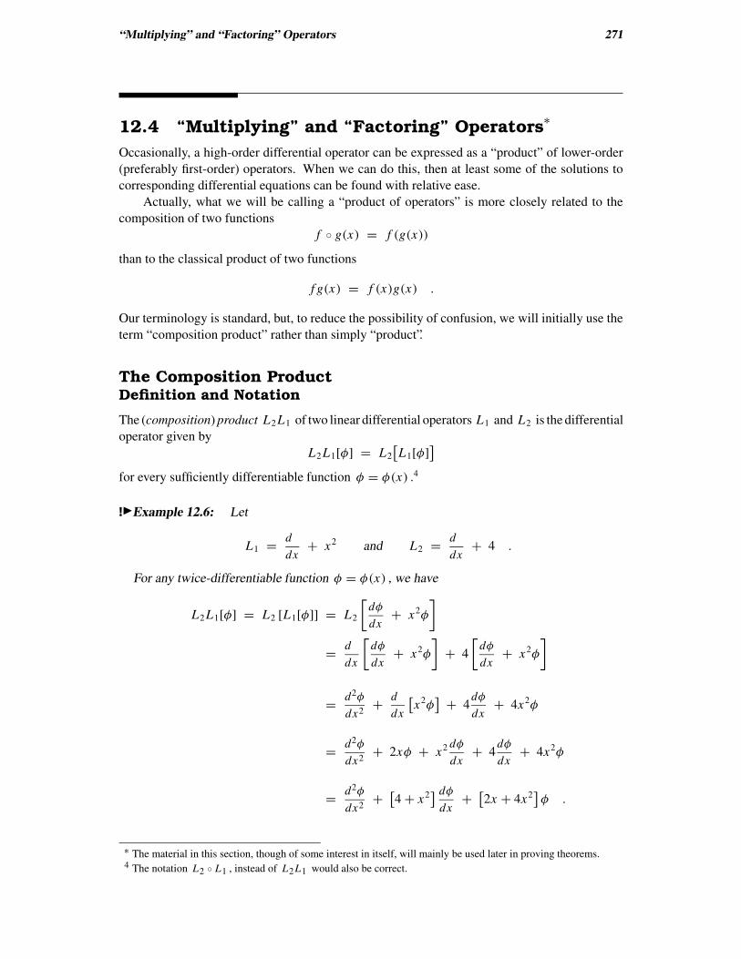
!◮Example 12.6: Let
L1 = d
dx+ x2 and L2 = d
dx+ 4 .
For any twice-differentiable function φ = φ(x) , we have
L2L1[φ] = L2 [L1[φ]] = L2
[
dφ
dx+ x2φ
]
= d
dx
[
dφ
dx+ x2φ
]
+ 4
[
dφ
dx+ x2φ
]
= d2φ
dx2+ d
dx
[
x2φ]
+ 4dφ
dx+ 4x2φ
= d2φ
dx2+ 2xφ + x2 dφ
dx+ 4
dφ
dx+ 4x2φ
= d2φ
dx2+
[
4 + x2] dφ
dx+
[
2x + 4x2]
φ .
∗ The material in this section, though of some interest in itself, will mainly be used later in proving theorems.4 The notation L2 ∘ L1 , instead of L2L1 would also be correct.

272 Higher-Order Linear Equations: Definitions and Some Basic Theory
Cutting out the middle yields
L2L1[φ] = d2φ
dx2+
[
4 + x2] dφ
dx+
[
2x + 4x2]
φ
for every sufficiently differentiable function φ . Thus
L2L1 = d2
dx2+
[
4 + x2] d
dx+
[
2x + 4x2]
.
When we have formulas for our operators L1 and L2 , it will often be convenient to replace
the symbols “ L1 ” and “ L2 ” with their formulas enclosed in parentheses. We will also enclose
any function φ being “plugged into” the operators with square brackets, “ [φ] ”. This will be
called the product notation.5
!◮Example 12.7: Using the product notation, let us recompute L2L1 for
L1 = d
dx+ x2 and L2 = d
dx+ 4 .
Letting φ = φ(x) be any twice-differentiable function,
(
d
dx+ 4
) (
d
dx+ x2
)
[φ] =(
d
dx+ 4
)[
dφ
dx+ x2φ
]
= d
dx
[
dφ
dx+ x2φ
]
+ 4
[
dφ
dx+ x2φ
]
= d2φ
dx2+ d
dx
[
x2φ]
+ 4dφ
dx+ 4x2φ
= d2φ
dx2+ 2xφ + x2 dφ
dx+ 4
dφ
dx+ 4x2φ
= d2φ
dx2+
[
4 + x2] dφ
dx+
[
2x + 4x2]
φ .
So,
L2L1 =(
d
dx+ 4
) (
d
dx+ x2
)
= d2
dx2+
[
4 + x2] d
dx+
[
2x + 4x2]
,
just as derived in the previous example.
5 Many authors do not enclose “the function being plugged in” in square brackets, and just write L2L1φ . We are
avoiding that because it does not explicitly distinguish between “φ as a function being plugged in” and “φ as an
operator, itself”. For the first, L2L1φ means the function you get from computing L2
[
L1[φ]]
. For the second,
L2 L1φ means the operator such that, for any sufficiently differentiable function ψ ,
L2
[
L1 [φ[ψ]]]
= L2
[
L1[φψ]]
,
The two possible interpretations for L2L1φ are not the same.
“Multiplying” and “Factoring” Operators 273
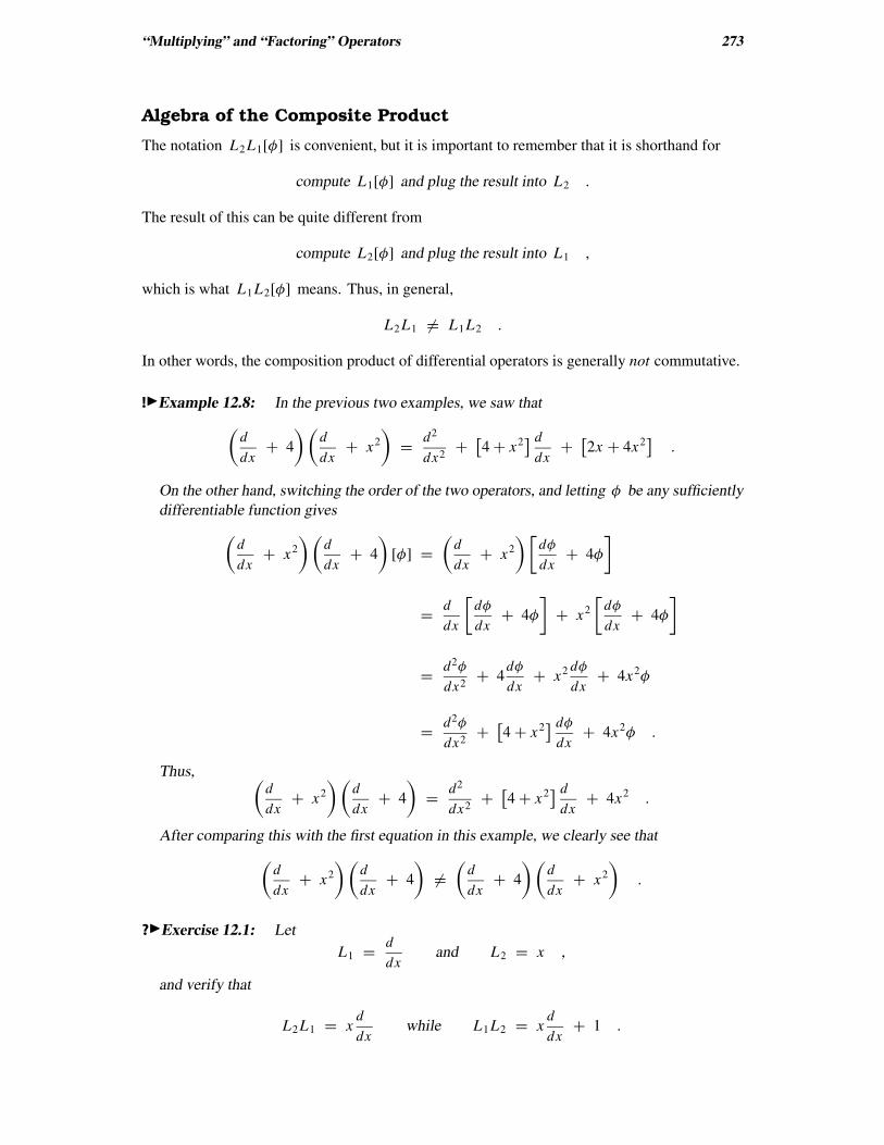
Algebra of the Composite Product
The notation L2L1[φ] is convenient, but it is important to remember that it is shorthand for
compute L1[φ] and plug the result into L2 .
The result of this can be quite different from
compute L2[φ] and plug the result into L1 ,
which is what L1L2[φ] means. Thus, in general,
L2 L1 6= L1L2 .
In other words, the composition product of differential operators is generally not commutative.
!◮Example 12.8: In the previous two examples, we saw that
(
d
dx+ 4
) (
d
dx+ x2
)
= d2
dx2+
[
4 + x2] d
dx+
[
2x + 4x2]
.
On the other hand, switching the order of the two operators, and letting φ be any sufficiently
differentiable function gives
(
d
dx+ x2
) (
d
dx+ 4
)
[φ] =(
d
dx+ x2
)[
dφ
dx+ 4φ
]
= d
dx
[
dφ
dx+ 4φ
]
+ x2
[
dφ
dx+ 4φ
]
= d2φ
dx2+ 4
dφ
dx+ x2 dφ
dx+ 4x2φ
= d2φ
dx2+
[
4 + x2] dφ
dx+ 4x2φ .
Thus,(
d
dx+ x2
) (
d
dx+ 4
)
= d2
dx2+
[
4 + x2] d
dx+ 4x2 .
After comparing this with the first equation in this example, we clearly see that
(
d
dx+ x2
) (
d
dx+ 4
)
6=(
d
dx+ 4
)(
d
dx+ x2
)
.
?◮Exercise 12.1: Let
L1 = d
dxand L2 = x ,
and verify that
L2L1 = xd
dxwhile L1L2 = x
d
dx+ 1 .
274 Higher-Order Linear Equations: Definitions and Some Basic Theory
Later (in chapters 18 and 21) we will be dealing with special situations in which the compo-
sition product is commutative. In fact, the material we are now developing will be most useful
verifying certain theorems involving those situations. In the meantime, just remember that, in
general,
L2 L1 6= L1L2 .
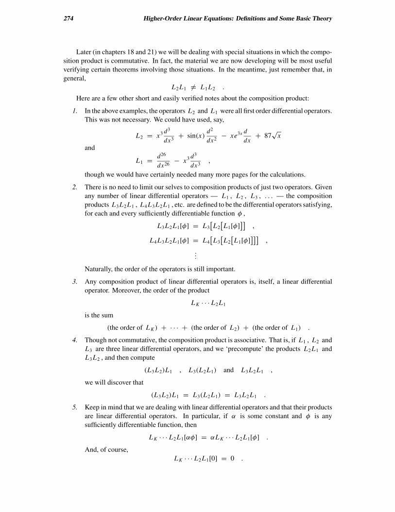
Here are a few other short and easily verified notes about the composition product:
1. In the above examples, the operators L2 and L1 were all first order differential operators.
This was not necessary. We could have used, say,
L2 = x3 d3
dx3+ sin(x)
d2
dx2− xe3x d
dx+ 87
√x
and
L1 = d26
dx26− x3 d3
dx3,
though we would have certainly needed many more pages for the calculations.
2. There is no need to limit our selves to composition products of just two operators. Given
any number of linear differential operators — L1 , L2 , L3 , . . . — the composition
products L3L2L1 , L4L3L2 L1 , etc. are defined to be the differential operators satisfying,
for each and every sufficiently differentiable function φ ,
L3L2 L1[φ] = L3
[
L2
[
L1[φ]]]
,
L4L3L2 L1[φ] = L4
[
L3
[
L2
[
L1[φ]]]]
,
...
Naturally, the order of the operators is still important.
3. Any composition product of linear differential operators is, itself, a linear differential
operator. Moreover, the order of the product
L K · · · L2L1
is the sum
(the order of L K ) + · · · + (the order of L2) + (the order of L1) .
4. Though not commutative, the composition product is associative. That is, if L1 , L2 and
L3 are three linear differential operators, and we ‘precompute’ the products L2 L1 and
L3L2 , and then compute
(L3L2)L1 , L3(L2L1) and L3L2 L1 ,
we will discover that
(L3L2)L1 = L3(L2L1) = L3L2 L1 .
5. Keep in mind that we are dealing with linear differential operators and that their products
are linear differential operators. In particular, if α is some constant and φ is any
sufficiently differentiable function, then
L K · · · L2L1[αφ] = αL K · · · L2 L1[φ] .
And, of course,
L K · · · L2L1[0] = 0 .
“Multiplying” and “Factoring” Operators 275
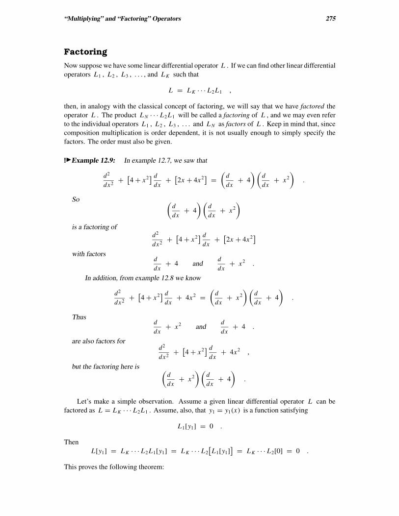
Factoring
Now suppose we have some linear differential operator L . If we can find other linear differential
operators L1 , L2 , L3 , . . . , and L K such that
L = L K · · · L2L1 ,
then, in analogy with the classical concept of factoring, we will say that we have factored the
operator L . The product L N · · · L2L1 will be called a factoring of L , and we may even refer
to the individual operators L1 , L2 , L3 , . . . and L N as factors of L . Keep in mind that, since
composition multiplication is order dependent, it is not usually enough to simply specify the
factors. The order must also be given.
!◮Example 12.9: In example 12.7, we saw that
d2
dx2+
[
4 + x2] d
dx+
[
2x + 4x2]
=(
d
dx+ 4
) (
d
dx+ x2
)
.
So(
d
dx+ 4
)(
d
dx+ x2
)
is a factoring ofd2
dx2+
[
4 + x2] d
dx+
[
2x + 4x2]
with factorsd
dx+ 4 and
d
dx+ x2 .
In addition, from example 12.8 we know
d2
dx2+
[
4 + x2] d
dx+ 4x2 =
(
d
dx+ x2
)(
d
dx+ 4
)
.
Thusd
dx+ x2 and
d
dx+ 4 .
are also factors ford2
dx2+
[
4 + x2] d
dx+ 4x2 ,
but the factoring here is(
d
dx+ x2
)(
d
dx+ 4
)
.
Let’s make a simple observation. Assume a given linear differential operator L can be
factored as L = L K · · · L2L1 . Assume, also, that y1 = y1(x) is a function satisfying
L1[y1] = 0 .
Then
L[y1] = L K · · · L2 L1[y1] = L K · · · L2
[
L1[y1]]
= L K · · · L2[0] = 0 .
This proves the following theorem:
276 Higher-Order Linear Equations: Definitions and Some Basic Theory
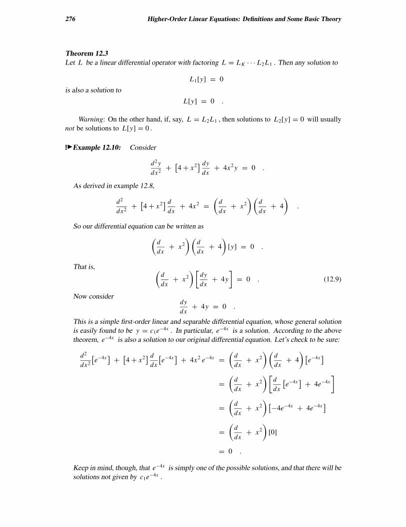
Theorem 12.3
Let L be a linear differential operator with factoring L = L K · · · L2 L1 . Then any solution to
L1[y] = 0
is also a solution to
L[y] = 0 .
Warning: On the other hand, if, say, L = L2L1 , then solutions to L2[y] = 0 will usually
not be solutions to L[y] = 0 .
!◮Example 12.10: Consider
d2 y
dx2+
[
4 + x2] dy
dx+ 4x2 y = 0 .
As derived in example 12.8,
d2
dx2+
[
4 + x2] d
dx+ 4x2 =
(
d
dx+ x2
)(
d
dx+ 4
)
.
So our differential equation can be written as
(
d
dx+ x2
)(
d
dx+ 4
)
[y] = 0 .
That is,(
d
dx+ x2
)[
dy
dx+ 4y
]
= 0 . (12.9)
Now considerdy
dx+ 4y = 0 .
This is a simple first-order linear and separable differential equation, whose general solution
is easily found to be y = c1e−4x . In particular, e−4x is a solution. According to the above
theorem, e−4x is also a solution to our original differential equation. Let’s check to be sure:
d2
dx2
[
e−4x]
+[
4 + x2] d
dx
[
e−4x]
+ 4x2 e−4x =(
d
dx+ x2
)(
d
dx+ 4
)
[
e−4x]
=(
d
dx+ x2
)[
d
dx
[
e−4x]
+ 4e−4x
]
=(
d
dx+ x2
)
[
−4e−4x + 4e−4x]
=(
d
dx+ x2
)
[0]
= 0 .
Keep in mind, though, that e−4x is simply one of the possible solutions, and that there will be
solutions not given by c1e−4x .
Additional Exercises 277
Unfortunately, unless it is of an exceptionally simple type (such as considered in chapter
18), factoring a linear differential operator is a very nontrivial problem. And even with those
simple types that we will be able to factor, we will find the main value of the above to be in
deriving even simpler methods for finding solutions. Consequently, in practice, you should not
expect to be solving many differential equations via “factoring”.
Additional Exercises
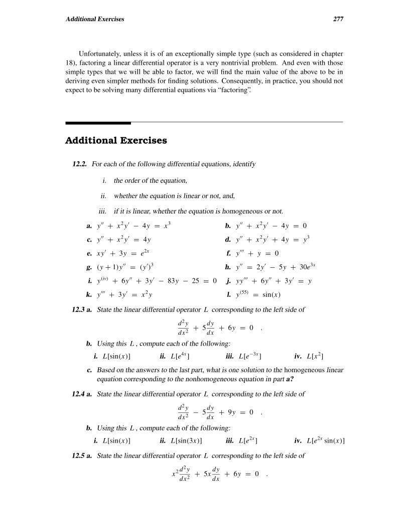
12.2. For each of the following differential equations, identify
i. the order of the equation,
ii. whether the equation is linear or not, and,
iii. if it is linear, whether the equation is homogeneous or not.
a. y′′ + x2 y′ − 4y = x3 b. y′′ + x2 y′ − 4y = 0
c. y′′ + x2 y′ = 4y d. y′′ + x2 y′ + 4y = y3
e. xy′ + 3y = e2x f. y′′′ + y = 0
g. (y + 1)y′′ = (y′)3 h. y′′ = 2y′ − 5y + 30e3x
i. y(iv) + 6y′′ + 3y′ − 83y − 25 = 0 j. yy′′′ + 6y′′ + 3y′ = y
k. y′′′ + 3y′ = x2 y l. y(55) = sin(x)
12.3 a. State the linear differential operator L corresponding to the left side of
d2 y
dx2+ 5
dy
dx+ 6y = 0 .
b. Using this L , compute each of the following:
i. L[sin(x)] ii. L[e4x ] iii. L[e−3x ] iv. L[x2]
c. Based on the answers to the last part, what is one solution to the homogeneous linear
equation corresponding to the nonhomogeneous equation in part a?
12.4 a. State the linear differential operator L corresponding to the left side of
d2 y
dx2− 5
dy
dx+ 9y = 0 .
b. Using this L , compute each of the following:
i. L[sin(x)] ii. L[sin(3x)] iii. L[e2x ] iv. L[e2x sin(x)]
12.5 a. State the linear differential operator L corresponding to the left side of
x2 d2 y
dx2+ 5x
dy
dx+ 6y = 0 .
278 Higher-Order Linear Equations: Definitions and Some Basic Theory
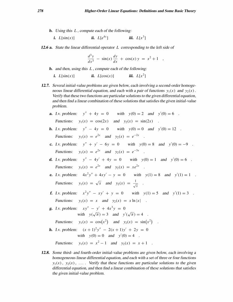
b. Using this L , compute each of the following:
i. L[sin(x)] ii. L[e4x ] iii. L[x3]
12.6 a. State the linear differential operator L corresponding to the left side of
d3 y
dx3− sin(x)
dy
dx+ cos(x) y = x2 + 1 ,
b. and then, using this L , compute each of the following:
i. L[sin(x)] ii. L[cos(x)] iii. L[x2]
12.7. Several initial-value problems are given below, each involving a second-order homoge-
neous linear differential equation, and each with a pair of functions y1(x) and y2(x) .
Verify that these two functions are particular solutions to the given differential equation,
and then find a linear combination of these solutions that satisfies the given initial-value
problem.
a. I.v. problem: y′′ + 4y = 0 with y(0) = 2 and y′(0) = 6 .
Functions: y1(x) = cos(2x) and y2(x) = sin(2x) .
b. I.v. problem: y′′ − 4y = 0 with y(0) = 0 and y′(0) = 12 .
Functions: y1(x) = e2x and y2(x) = e−2x .
c. I.v. problem: y′′ + y′ − 6y = 0 with y(0) = 8 and y′(0) = −9 .
Functions: y1(x) = e2x and y2(x) = e−3x .
d. I.v. problem: y′′ − 4y′ + 4y = 0 with y(0) = 1 and y′(0) = 6 .
Functions: y1(x) = e2x and y2(x) = xe2x .
e. I.v. problem: 4x2 y′′ + 4xy′ − y = 0 with y(1) = 8 and y′(1) = 1 .
Functions: y1(x) =√
x and y2(x) = 1√
x.
f. I.v. problem: x2 y′′ − xy′ + y = 0 with y(1) = 5 and y′(1) = 3 .
Functions: y1(x) = x and y2(x) = x ln |x | .
g. I.v. problem: xy′′ − y′ + 4x3 y = 0
with y(√π) = 3 and y′(
√π) = 4 .
Functions: y1(x) = cos(
x2)
and y2(x) = sin(
x2)
.
h. I.v. problem: (x + 1)2 y′′ − 2(x + 1)y′ + 2y = 0
with y(0) = 0 and y′(0) = 4 .
Functions: y1(x) = x2 − 1 and y2(x) = x + 1 .
12.8. Some third- and fourth-order initial-value problems are given below, each involving a
homogeneous linear differential equation, and each with a set of three or four functions
y1(x) , y2(x) , . . . . Verify that these functions are particular solutions to the given
differential equation, and then find a linear combination of these solutions that satisfies
the given initial-value problem.
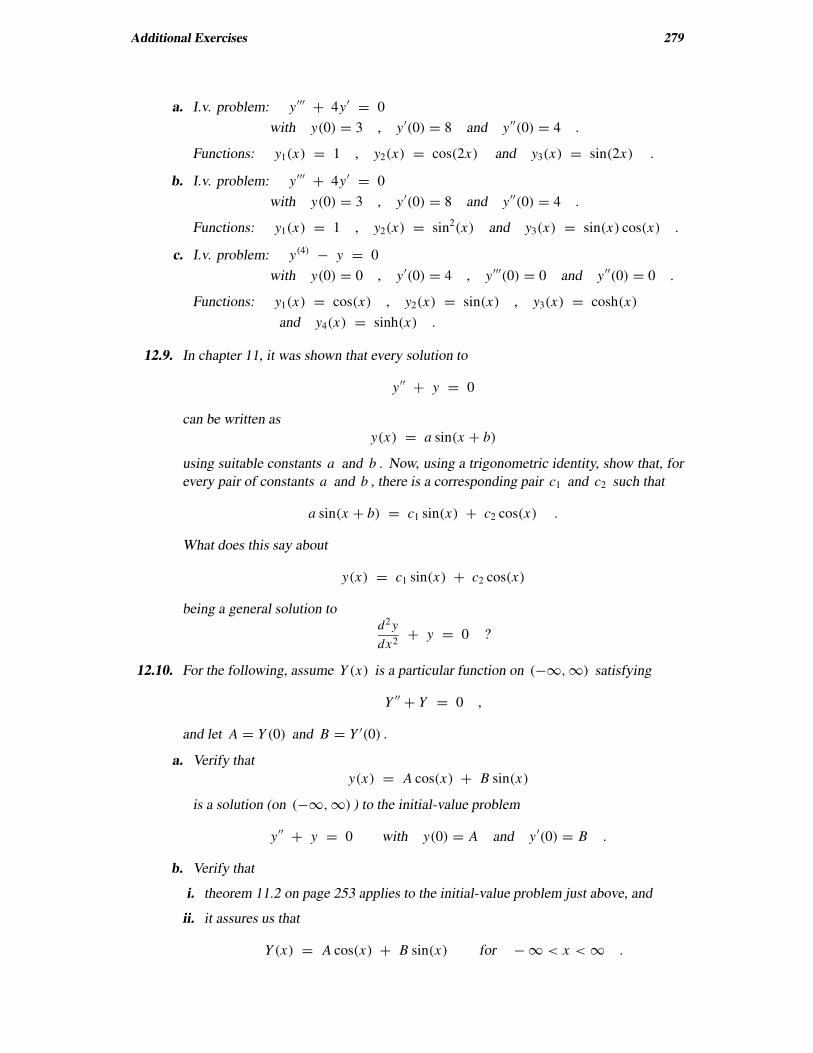
Additional Exercises 279
a. I.v. problem: y′′′ + 4y′ = 0
with y(0) = 3 , y′(0) = 8 and y′′(0) = 4 .
Functions: y1(x) = 1 , y2(x) = cos(2x) and y3(x) = sin(2x) .
b. I.v. problem: y′′′ + 4y′ = 0
with y(0) = 3 , y′(0) = 8 and y′′(0) = 4 .
Functions: y1(x) = 1 , y2(x) = sin2(x) and y3(x) = sin(x) cos(x) .
c. I.v. problem: y(4) − y = 0
with y(0) = 0 , y′(0) = 4 , y′′′(0) = 0 and y′′(0) = 0 .
Functions: y1(x) = cos(x) , y2(x) = sin(x) , y3(x) = cosh(x)
and y4(x) = sinh(x) .
12.9. In chapter 11, it was shown that every solution to
y′′ + y = 0
can be written as
y(x) = a sin(x + b)
using suitable constants a and b . Now, using a trigonometric identity, show that, for
every pair of constants a and b , there is a corresponding pair c1 and c2 such that
a sin(x + b) = c1 sin(x) + c2 cos(x) .
What does this say about
y(x) = c1 sin(x) + c2 cos(x)
being a general solution tod2 y
dx2+ y = 0 ?
12.10. For the following, assume Y (x) is a particular function on (−∞,∞) satisfying
Y ′′ + Y = 0 ,
and let A = Y (0) and B = Y ′(0) .
a. Verify that
y(x) = A cos(x) + B sin(x)
is a solution (on (−∞,∞) ) to the initial-value problem
y′′ + y = 0 with y(0) = A and y′(0) = B .
b. Verify that
i. theorem 11.2 on page 253 applies to the initial-value problem just above, and
ii. it assures us that
Y (x) = A cos(x) + B sin(x) for − ∞ < x < ∞ .
280 Higher-Order Linear Equations: Definitions and Some Basic Theory
c. What does all this tell us about {cos(x), sin(x)} being a fundamental set of solutions
for
y′′ + y = 0 ?
12.11. Several choices for linear differential operators L1 and L2 are given below. For each
choice, compute L2 L1 and L1L2 .
a. L1 = d
dx+ x and L2 = d
dx− x
b. L1 = d
dx+ x2 and L2 = d
dx+ x3
c. L1 = xd
dx+ 3 and L2 = d
dx+ 2x
d. L1 = d2
dx2and L2 = x
e. L1 = d2
dx2and L2 = x3
f. L1 = d2
dx2and L2 = sin(x)
12.12. Compute the following composition products:
a.
(
d
dx+ 2
) (
d
dx+ 3
)
b.
(
xd
dx+ 2
)(
xd
dx+ 3
)
c.
(
xd
dx+ 4
) (
d
dx+ 1
x
)
d.
(
d
dx+ 4x
)(
d
dx+ 1
x
)
e.
(
d
dx+ 1
x
) (
d
dx+ 4x
)
f.
(
d
dx+ 5x2
)2
g.
(
d
dx+ x2
) (
d2
dx2+ d
dx
)
h.
(
d2
dx2+ d
dx
)(
d
dx+ x2
)
12.13. Verify that
d2
dx2+ [sin(x)− 3]d
dx− 3 sin(x) =
(
d
dx+ sin(x)
)(
d
dx− 3
)
,
and, using this factorization, find one solution to
d2 y
dx2+ [sin(x)− 3]dy
dx− 3 sin(x)y = 0 .
12.14. Verify that
d2
dx2+ x
d
dx+
[
2 − 2x2]
=(
d
dx− x
)(
d
dx+ 2x
)
,
and, using this factorization, find one solution to
d2 y
dx2+ x
dy
dx+
[
2 − 2x2]
y = 0 .
Additional Exercises 281
12.15. Verify that
x2 d2
dx2− 7x
d
dx+ 16 =
(
xd
dx− 4
)2
,
and, using this factorization, find one solution to
x2 d2 y
dx2− 7x
dy
dx+ 16y = 0 .