Higher-Order Income Risk and SocialInsurance Policy Over the Business Cycle

Christopher Busch

∗David Domeij

†Fatih Guvenen

‡Rocio Madera

§

April 21, 2015

Preliminary and Incomplete. Comments Welcome.

Abstract

This paper studies the business-cycle variation in higher-order income risk—i.e.,risks that are captured by moments higher than the variance. A key focus of ouranalysis is the extent to which such risks can be smoothed within households orwith government social insurance policies. To provide a broad perspective on thesequestions, we study panel data on individuals and households from the UnitedStates, Germany, and Sweden, covering more than three decades of data for eachcountry. We find that the underlying variation in higher-order risk is remarkablysimilar across these countries that differ in many details of their labor markets. Inparticular, in all three countries, the variance of earnings changes is almost entirelyconstant over the business cycle, whereas the skewness of these shocks becomesmuch more negative in recessions. Government provided insurance, in the form ofunemployment insurance, welfare benefits, aid to low income households, and thelike, plays a more important role reducing downside risk in all three countries; theeffectiveness is weakest in the United States, and most pronounced in Germany. Wecalculate that the welfare benefits of social insurance policies for stabilizing higher-order income risk over the business cycle range from 1% of annual consumption forthe United States to 5% for Germany.

JEL Codes: D31, E24, E32, H31Keywords: Idiosyncratic income risk, countercyclical risk, business cycles,

skewness, social insurance policy.

∗CMR, University of Cologne; busch@wiso.uni-koeln.de†Stockholm School of Economics; david.domeij@hhs.se‡University of Minnesota, FRB of Minneapolis, and NBER; guvenen@umn.edu; www.fguvenen.com

§University of Minnesota; made0088@umn.edu

1 Introduction

This paper studies how higher-order income risk varies over the business cycle as wellas the extent to which such risks can be smoothed within households or with governmentsocial insurance policies. By higher-order income risk, we refer to risks that are capturedby not only the variance of income shocks, but also their skewness and kurtosis. Thesehigher order moments of the data can be a major source of risk for individuals as weshow in this paper.

To provide a broad perspective on these questions, we study panel data on individualsand households from the United States, Germany, and Sweden, covering more thanthree decades of data for each country. It is useful to begin by putting our analysisin context. A broad range of empirical evidence indicates that idiosyncratic incomerisk rises in recessions. Earlier work in the literature was based on small survey-basedpanel datasets, such as the Panel Study of Income Dynamics (PSID), which requiredresearchers to make parametric assumptions to obtain identification. The earlier studiesin the literature have restricted attention to the changes in the mean and variance ofincome shocks and concluded that the variance of income shocks is countercyclical (e.g.,Storesletten et al. (2004)). In recent work, Guvenen et al. (2014) used a very large paneldataset on earnings histories from the U.S. Social Security Administration (SSA) records.Using non-parametric techniques, they found that the variance of income shocks is verystable over time and is robustly acyclical, whereas the left-skewness of shocks variessignificantly over time in a countercyclical fashion.

Despite important advantages, the SSA data also have three shortcomings: (i) earn-ings data are available only for individuals, and it is not possible to link householdmembers to each other, (ii) no information is available on taxes and transfers (unem-ployment insurance, welfare payments, gifts, etc.), and (iii) no information is availableon skills/education. Furthermore, Guvenen et al. (2014) focus on males with no corre-sponding information on women.

This paper makes three contributions. First, applying non-parametric techniquesand using robust statistics, we document that the variance of individual labor earningsgrowth is flat and acyclical in all three countries, whereas the left-skewness of shocksis strongly countercyclical. Therefore, we conclude that applying the same method tosurvey and administrative data yields the same substantive conclusions.

1

Second, we find that the underlying variation in higher-order risk is remarkably simi-lar across these countries that differ in many details of their labor markets. In particular,in all three countries, the variance of earnings shocks is almost entirely constant over thebusiness cycle, whereas the skewness of these shocks becomes significantly more negativein recessions.

Third, we find that insurance provided within households or by the government playsan important role in reducing downside risk, but that how and to what extent differsbetween the countries. Within-household provided insurance reduces the countercycli-cality in the skewness of earnings in Sweden, but evidence of within-household insuranceis much weaker in United States and in Germany. Government provided insurance, inthe form of unemployment insurance, welfare benefits, aid to low income households, andthe like, plays a more important role in all three countries; the effectiveness is weakestin the United States, and strongest in Germany.

The paper is organized as follows. The next section discusses the data sources, andSection 3 describes the empirical approach. Section 4 presents the results for gross(before-government) individual earnings and examines how the patterns of cyclicalityvary by gender, education, and type of employment. Section 5 expands the analysis tohouseholds and includes various types of government social insurance policies to examinetheir impact on the cyclicality of higher-order risk. Section 6 presents a simple (andpreliminary) welfare analysis to quantify the potential welfare benefits of governments’social insurance policies in the three countries we study. Section 7 concludes.

1.1 Related Literature

[To be added]

2 The Data

This section provides an overview of the data sets we use in our empirical analysis,the sample selection criteria, as well as the variables used in the subsequent empiricalanalyses. Given the diversity of our data sources, we relegate the details to Appendix A.Briefly, we employ four longitudinal data sets corresponding to three different countries:the Panel Study of Income Dynamics (PSID) for the United States, covering 1976 to

2

2010;1 the Sample of Integrated Labour Market Biographies (SIAB2) and the GermanSocio-Economic Panel (SOEP) for Germany, covering 1976 to 2010 and 1984 to 2011,respectively; and the Longitudinal Individual Data Base (LINDA) for Sweden, covering1979 to 2010. The PSID and the SOEP are survey-based data sets. The PSID hasa yearly sample of approximately 2000 households in the core sample, which is repre-sentative of the U.S. population; the SOEP started with about 10,000 individuals (or5,000 households) in 1984 and, after several refreshments, covers about 18,000 individuals(10,500 households) in 2011.3

The SIAB is based on administrative social security records and our initial samplecovers on average 370,000 individuals per year. It excludes civil servants, students andself-employed, which make about 20% of the workforce. From the perspective of ouranalysis, the SIAB has two caveats: (i) income is top-coded at the limit of incomesubject to social security contributions, and (ii) individuals cannot be linked to eachother, which prohibits identification of households. We deal with (i) by fitting a Paretodistribution to the upper tail of the wage distribution (following Daly et al. (2014); seeAppendix A.3 for details) and with (ii) by using data from SOEP for all household-level analyses. Throughout the analysis we focus on West Germany, which for simplicitywe refer to as Germany. LINDA is compiled from administrative sources (the IncomeRegister) and tracks a representative sample with approximately 300,000 individuals peryear.

For each country, we consider three samples: two at the individual level—one formales and one for females—and one at the household level. The samples are constructedas revolving panels: for a given statistic computed based on the time difference betweenyears t and t+ k, the panel contains individuals who are aged 25 to 59 in periods t andt + k (k = 1 or 5) and have yearly labor earnings above a minimum threshold in bothyears. This threshold is defined as the earnings level that corresponds to 520 hours ofemployment at half the legal minimum wage, which is about $1885 US dollars for the

1The PSID contains information since 1967. We choose our benchmark sample to start in 1976 dueto the poor coverage of income transfers before the 1977 wave. We complement our results using alonger period whenever possible and pertinent.

2We use the factually anonymous scientific use file SIAB-R7510, which is a 2% draw from theIntegrated Employment Biographies data of the Institute for Employment Research (IAB).

3These numbers refer to observations after cleaning but before sample selection. Only the represen-tative SRC sample is considered in the PSID. The immigrant sample and high income sample of theSOEP are not used, because they cover only sub-periods.

3

United States in 2010.4 To avoid possible outliers, we exclude the top 1% of earningsobservations in the PSID and SOEP, but not in LINDA (which is from administrativesources). For each individual, we record age, gender, education, and labor earnings.

The household sample is constructed by imposing the same criteria on the householdhead and adding specific requirements at the household level. More specifically, a house-hold is included in our sample if it has at least two adult members, one of them beingthe household head,5 that satisfy the age criterion and household income that satisfiesthe income criteria. At the household level, we will analyze several income measures.We start with labor earnings and then add various transfers, taxes, and capital income.To ensure that the sample is consistent across our analyses, the condition that earningsexceed our minimum threshold is imposed on the minimum earnings across all house-hold income measures. Household earnings are converted into adult-equivalent units bydividing by the square root of household size.

Classifying Expansions and Recessions

For the United States, the classification of expansionary and recessionary episodesis based on the NBER peak and trough dates, with small timing variations. Given thetime span covered by our sample, we classify the following years as recessions: 1980–1983,1991–92, 2001–2002, and 2008–2010. The main difference compared to the NBER listis that we treat the 1980–1983 period as a single “double-dip” recession because of theshort duration of the intervening expansion and the lack of recovery in the unemploymentrate. Based on this classification, there are four expansions and four recessions duringour sample period.

For both Germany and Sweden, we base the dating of expansions and recessionson data from the Economic Cycle Research Institute (ECRI), which applies the NBERmethodology to OECD countries since 1948. The classification is consistent with variousaggregate measures of the German and Swedish economies, respectively. In the timeperiod covered by the panel data, recession periods for Germany (peak to trough) are

4For the United States, we use the federal minimum wage. There is no official minimum wage inSweden or Germany during this period. For Germany, we a take a minimum threshold of 3 Euros (inyear 2000 Euros) for the hourly wage. For Sweden, the effective hourly minimum wage via labor marketagreements was around SEK 75 in 2004 (Skedinger, 2007). For other years, we adjust the minimumwage by calculating the mean real earnings for each year, estimating a linear time trend for these meansand removing that time trend from the SEK 75 minimum wage.

5In PSID and SOEP the head of a household is defined within the data set. In LINDA, the head ofa household is defined as the sampled male.

4

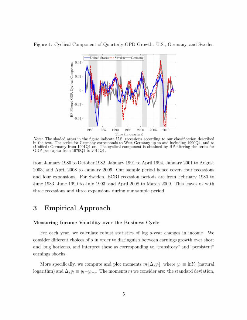
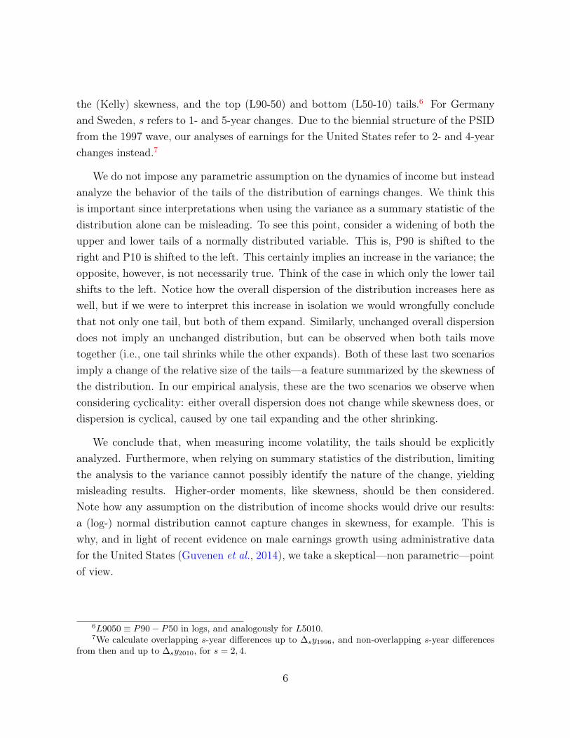
Figure 1: Cyclical Component of Quarterly GPD Growth: U.S., Germany, and Sweden

Time (in quarters)1980 1985 1990 1995 2000 2005 2010

HP

-Fil

tere

d G

DP

, C

ycl

ical

Com

ponen

t

-0.04

-0.02

0

0.02

0.04

United States Sweden Germany

Note: The shaded areas in the figure indicate U.S. recessions according to our classification describedin the text. The series for Germany corresponds to West Germany up to and including 1990Q4, and to(Unified) Germany from 1991Q1 on. The cyclical component is obtained by HP-filtering the series forGDP per capita from 1970Q1 to 2014Q1.

from January 1980 to October 1982, January 1991 to April 1994, January 2001 to August2003, and April 2008 to January 2009. Our sample period hence covers four recessionsand four expansions. For Sweden, ECRI recession periods are from February 1980 toJune 1983, June 1990 to July 1993, and April 2008 to March 2009. This leaves us withthree recessions and three expansions during our sample period.

3 Empirical Approach

Measuring Income Volatility over the Business Cycle

For each year, we calculate robust statistics of log s-year changes in income. Weconsider different choices of s in order to distinguish between earnings growth over shortand long horizons, and interpret these as corresponding to “transitory” and “persistent”earnings shocks.

More specifically, we compute and plot moments m [�syt], where yt ⌘ lnYt (naturallogarithm) and �syt ⌘ yt�yt�s. The moments m we consider are: the standard deviation,

5

the (Kelly) skewness, and the top (L90-50) and bottom (L50-10) tails.6 For Germanyand Sweden, s refers to 1- and 5-year changes. Due to the biennial structure of the PSIDfrom the 1997 wave, our analyses of earnings for the United States refer to 2- and 4-yearchanges instead.7

We do not impose any parametric assumption on the dynamics of income but insteadanalyze the behavior of the tails of the distribution of earnings changes. We think thisis important since interpretations when using the variance as a summary statistic of thedistribution alone can be misleading. To see this point, consider a widening of both theupper and lower tails of a normally distributed variable. This is, P90 is shifted to theright and P10 is shifted to the left. This certainly implies an increase in the variance; theopposite, however, is not necessarily true. Think of the case in which only the lower tailshifts to the left. Notice how the overall dispersion of the distribution increases here aswell, but if we were to interpret this increase in isolation we would wrongfully concludethat not only one tail, but both of them expand. Similarly, unchanged overall dispersiondoes not imply an unchanged distribution, but can be observed when both tails movetogether (i.e., one tail shrinks while the other expands). Both of these last two scenariosimply a change of the relative size of the tails—a feature summarized by the skewness ofthe distribution. In our empirical analysis, these are the two scenarios we observe whenconsidering cyclicality: either overall dispersion does not change while skewness does, ordispersion is cyclical, caused by one tail expanding and the other shrinking.

We conclude that, when measuring income volatility, the tails should be explicitlyanalyzed. Furthermore, when relying on summary statistics of the distribution, limitingthe analysis to the variance cannot possibly identify the nature of the change, yieldingmisleading results. Higher-order moments, like skewness, should be then considered.Note how any assumption on the distribution of income shocks would drive our results:a (log-) normal distribution cannot capture changes in skewness, for example. This iswhy, and in light of recent evidence on male earnings growth using administrative datafor the United States (Guvenen et al., 2014), we take a skeptical—non parametric—pointof view.

6L9050 ⌘ P90� P50 in logs, and analogously for L5010.7We calculate overlapping s-year differences up to �sy1996, and non-overlapping s-year differences

from then and up to �sy2010, for s = 2, 4.

6

Broadening the Definition of Business Cycles

Some of the important macroeconomic variables do not perfectly synchronize withexpansions and recessions, but their fluctuations might have an impact on earnings.For example, the U.S. stock market experienced a significant drop in 1987, during anexpansion, and we can see in the time series analysis how the third moment falls sharplyin that year. Similarly, the U.S. economy displayed an overall weakness in 1993–1994,which is evident in a range of economic variables, but these years are technically classifiedas part of an expansion by the NBER dating committee. Other examples are easy tofind for Germany and Sweden (e.g., 1996). Therefore, the main focus of our analysis willbe on the co-movement of higher-order moments of earnings changes with a continuousmeasure of business cycles.

For this part, we consider the four moments m defined above for the graphical analy-sis, and add two more. In particular, we compute correlations between GDP growth and(i) the standard deviation, (ii) the log differential between the 90th and 10th percentiles(L90-10), (iii) the skewness, measured as the third standardized moment, (iv) the Kelly’smeasure of skewness, and (v) the upper (L90-50) and (vi) lower (L50-10) tails. We usethe (natural) log growth rate of GDP—that is, �sGDPt ⌘ ln(GDP t)� ln(GDP t�s)—asour measure of aggregate fluctuations. Therefore, we consider the following regressionof each moment m of the log income change between t� s and t on a constant, a lineartime trend, and the log growth rate of GDP between year t� s and t :

m (�syt) = ↵ + �t+ �m ⇥�s(GDPt) + ut.

For a quantitative interpretation of the results reported in the next sections, TableI reports the short- and long-run volatility of GDP growth for each country and yearsample considered along the paper.

4 Empirical Results: Gross Individual Earnings

In this section, we examine the cyclical behavior of the dispersion and the skewnessof earnings changes in gross labor earnings for individuals. By gross earnings we mean aworker’s compensation from his/her employer before any kind of government interventionin the form of taxes, benefits, welfare, unemployment insurance, and so on. In the next

7

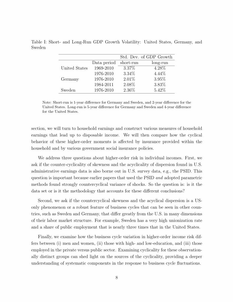
Table I: Short- and Long-Run GDP Growth Volatility: United States, Germany, andSweden

Std. Dev. of GDP GrowthData period short-run long-run

United States 1969-2010 3.37% 4.28%1976-2010 3.34% 4.44%

Germany 1976-2010 2.01% 3.95%1984-2011 2.08% 3.83%

Sweden 1976-2010 2.36% 5.42%

Note: Short-run is 1-year difference for Germany and Sweden, and 2-year difference for theUnited States. Long-run is 5-year difference for Germany and Sweden and 4-year differencefor the United States.

section, we will turn to household earnings and construct various measures of householdearnings that lead up to disposable income. We will then compare how the cyclicalbehavior of these higher-order moments is affected by insurance provided within thehousehold and by various government social insurance policies.

We address three questions about higher-order risk in individual incomes. First, weask if the counter-cyclicality of skewness and the acyclicality of dispersion found in U.S.administrative earnings data is also borne out in U.S. survey data, e.g., the PSID. Thisquestion is important because earlier papers that used the PSID and adopted parametricmethods found strongly countercyclical variance of shocks. So the question is: is it thedata set or is it the methodology that accounts for these different conclusions?

Second, we ask if the countercyclical skewness and the acyclical dispersion is a US-only phenomenon or a robust feature of business cycles that can be seen in other coun-tries, such as Sweden and Germany, that differ greatly from the U.S. in many dimensionsof their labor market structure. For example, Sweden has a very high unionization rateand a share of public employment that is nearly three times that in the United States.

Finally, we examine how the business cycle variation in higher-order income risk dif-fers between (i) men and women, (ii) those with high- and low-education, and (iii) thoseemployed in the private versus public sector. Examining cyclicality for these observation-ally distinct groups can shed light on the sources of the cyclicality, providing a deeperunderstanding of systematic components in the response to business cycle fluctuations.

8

To answer these questions, we start by computing correlations between earnings in-novations and GDP growth. Next, we plot some of the different moments over time andinspect their fluctuations over the business cycle.

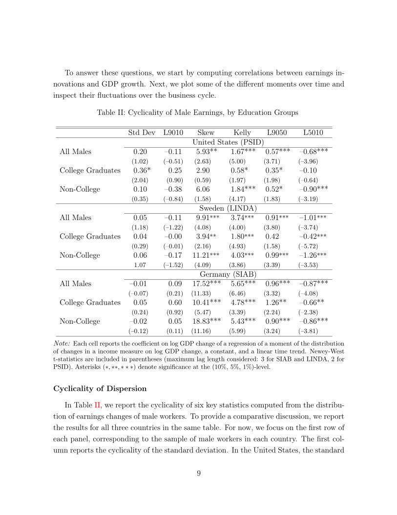
Table II: Cyclicality of Male Earnings, by Education Groups

Std Dev L9010 Skew Kelly L9050 L5010United States (PSID)

All Males 0.20 –0.11 5.93** 1.67*** 0.57*** –0.68***(1.02) (–0.51) (2.63) (5.00) (3.71) (–3.96)

College Graduates 0.36* 0.25 2.90 0.58* 0.35* –0.10(2.04) (0.90) (0.59) (1.97) (1.98) (–0.64)

Non-College 0.10 –0.38 6.06 1.84*** 0.52* –0.90***(0.35) (–0.84) (1.58) (4.17) (1.83) (–3.19)

Sweden (LINDA)All Males 0.05 –0.11 9.91*** 3.74*** 0.91*** –1.01***

(1.18) (–1.22) (4.08) (4.00) (3.80) (–3.74)College Graduates 0.04 –0.00 3.94** 1.80*** 0.42 –0.42***

(0.29) (–0.01) (2.16) (4.93) (1.58) (–5.72)Non-College 0.06 –0.17 11.21*** 4.03*** 0.99*** –1.26***

1.07 (–1.52) (4.09) (3.86) (3.39) (–3.53)Germany (SIAB)

All Males –0.01 0.09 17.52*** 5.65*** 0.96*** –0.87***(–0.07) (0.21) (11.33) (6.46) (3.32) (–4.08)

College Graduates 0.05 0.60 10.41*** 4.78*** 1.26** –0.66**(0.24) (0.92) (5.47) (3.39) (2.24) (–2.38)

Non-College –0.02 0.05 18.83*** 5.43*** 0.90*** –0.86***(–0.12) (0.11) (11.16) (5.99) (3.24) (–3.81)

Note: Each cell reports the coefficient on log GDP change of a regression of a moment of the distributionof changes in a income measure on log GDP change, a constant, and a linear time trend. Newey-Westt-statistics are included in parentheses (maximum lag length considered: 3 for SIAB and LINDA, 2 forPSID). Asterisks (⇤, ⇤⇤, ⇤ ⇤ ⇤) denote significance at the (10%, 5%, 1%)-level.

Cyclicality of Dispersion

In Table II, we report the cyclicality of six key statistics computed from the distribu-tion of earnings changes of male workers. To provide a comparative discussion, we reportthe results for all three countries in the same table. For now, we focus on the first row ofeach panel, corresponding to the sample of male workers in each country. The first col-umn reports the cyclicality of the standard deviation. In the United States, the standard

9

deviation is acyclical, as seen from the small (0.20) and statistically insignificant (t-statof 1.02) coefficient.8 In the next column, we report another measure of dispersion—thelog 90-10 differential—which is just as acyclical. Therefore, the PSID data is consistentwith the findings of Guvenen et al. (2014) regarding the acyclicality of dispersion fromthe much larger SSA administrative data.

A natural follow up question is whether this acyclicality is specific to the UnitedStates, or whether it also holds in Sweden and/or Germany, which in many ways have verydifferent labor markets. As seen in the first column of the middle panel, both measures ofdispersion are acyclical in Sweden, with very small and insignificant coefficients. Turningto Germany (bottom panel), standard deviation and L90-10 are again acyclical9.

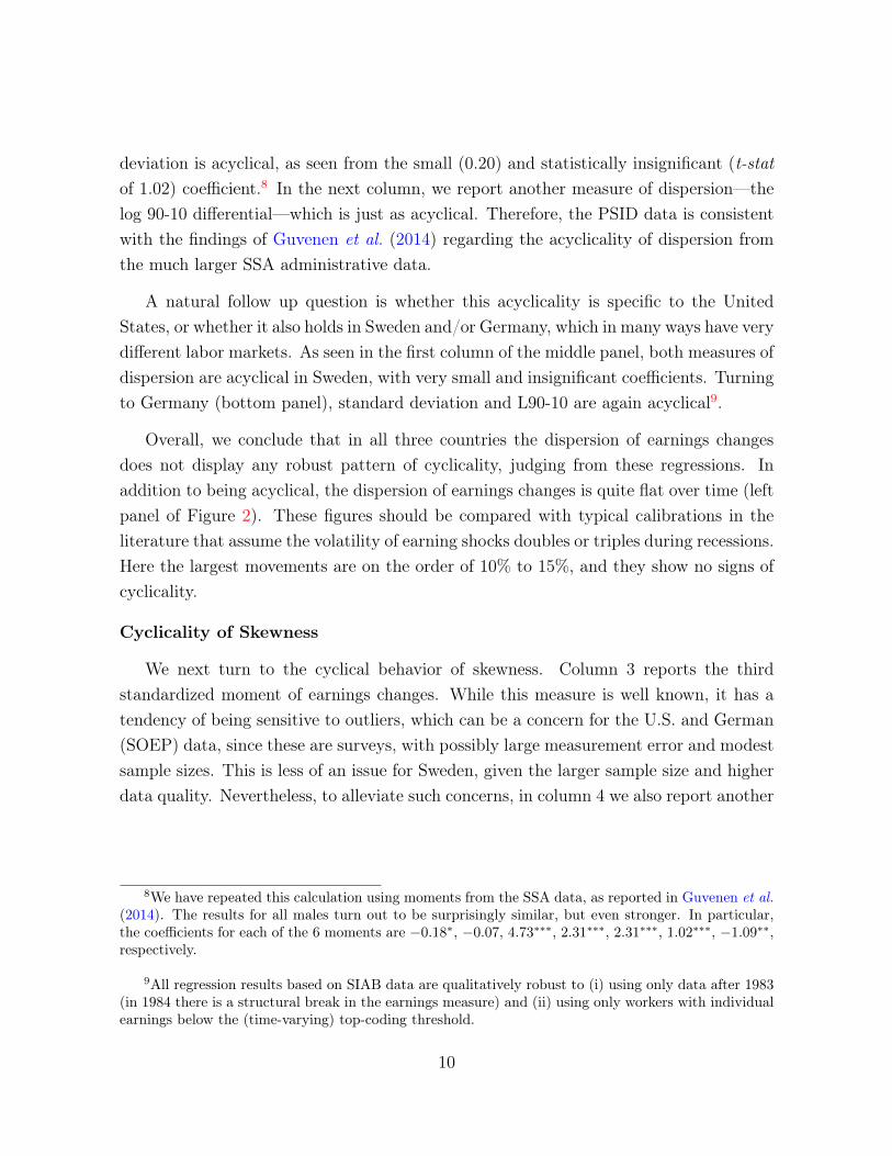
Overall, we conclude that in all three countries the dispersion of earnings changesdoes not display any robust pattern of cyclicality, judging from these regressions. Inaddition to being acyclical, the dispersion of earnings changes is quite flat over time (leftpanel of Figure 2). These figures should be compared with typical calibrations in theliterature that assume the volatility of earning shocks doubles or triples during recessions.Here the largest movements are on the order of 10% to 15%, and they show no signs ofcyclicality.

Cyclicality of Skewness

We next turn to the cyclical behavior of skewness. Column 3 reports the thirdstandardized moment of earnings changes. While this measure is well known, it has atendency of being sensitive to outliers, which can be a concern for the U.S. and German(SOEP) data, since these are surveys, with possibly large measurement error and modestsample sizes. This is less of an issue for Sweden, given the larger sample size and higherdata quality. Nevertheless, to alleviate such concerns, in column 4 we also report another

8We have repeated this calculation using moments from the SSA data, as reported in Guvenen et al.

(2014). The results for all males turn out to be surprisingly similar, but even stronger. In particular,the coefficients for each of the 6 moments are �0.18⇤, �0.07, 4.73⇤⇤⇤, 2.31⇤⇤⇤, 2.31⇤⇤⇤, 1.02⇤⇤⇤, �1.09⇤⇤,respectively.

9All regression results based on SIAB data are qualitatively robust to (i) using only data after 1983(in 1984 there is a structural break in the earnings measure) and (ii) using only workers with individualearnings below the (time-varying) top-coding threshold.

10

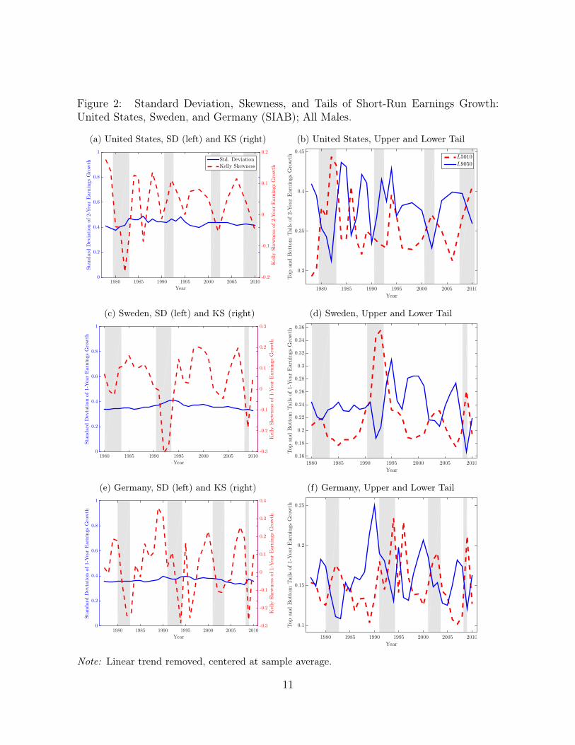
Figure 2: Standard Deviation, Skewness, and Tails of Short-Run Earnings Growth:United States, Sweden, and Germany (SIAB); All Males.

(a) United States, SD (left) and KS (right)

Year

1980 1985 1990 1995 2000 2005 2010

Standard

Deviationof2-YearEarningsGrowth

0

0.2

0.4

0.6

0.8

1

Std. Deviation

Kelly Skewness

Kelly

Skew

nessof2-YearEarningsGrowth

-0.2

-0.1

0

0.1

0.2

(b) United States, Upper and Lower Tail

Year

1980 1985 1990 1995 2000 2005 2010TopandBottom

Tailsof2-Y

earEarningsGrowth

0.3

0.35

0.4

0.45L5010

L9050

(c) Sweden, SD (left) and KS (right)

Year

1980 1985 1990 1995 2000 2005 2010

Standard

Deviationof1-YearEarningsGrowth

0

0.2

0.4

0.6

0.8

1

Kelly

Skew

nessof1-YearEarningsGrowth

-0.3

-0.2

-0.1

0

0.1

0.2

0.3

(d) Sweden, Upper and Lower Tail

Year

1980 1985 1990 1995 2000 2005 2010

TopandBottom

Tailsof1-Y

earEarningsGrowth

0.16

0.18

0.2

0.22

0.24

0.26

0.28

0.3

0.32

0.34

0.36

(e) Germany, SD (left) and KS (right)

Year

1980 1985 1990 1995 2000 2005 2010

Standard

Deviationof1-YearEarningsGrowth

0

0.2

0.4

0.6

0.8

1

Kelly

Skew

nessof1-YearEarningsGrowth

-0.3

-0.2

-0.1

0

0.1

0.2

0.3

0.4

(f) Germany, Upper and Lower Tail

Year

1980 1985 1990 1995 2000 2005 2010

TopandBottom

Tailsof1-Y

earEarningsGrowth

0.1

0.15

0.2

0.25

Note: Linear trend removed, centered at sample average.

11

measure of asymmetry, called Kelly’s skewness, defined as:

Sk =(P90� P50)� (P50� P10)

(P90� P10).

This measure has several attractive features. First, it is much less sensitive to extremeobservations, since it does not depend on observations beyond the 90th and 10th per-centiles of the distribution. This deals with the concern about potential outliers. Becauseof this advantage, it is our preferred measure of skewness, especially for the U.S. andGermany where measurement issues could be more important. Second, the particularvalue of Kelly’s skewness has a simple interpretation, in terms of the relative lengths ofthe top and bottom tails. In particular,

P90� P50

P90� P10= 0.5 +

Sk

2, (1)

which can be used to compute the fraction of overall dispersion (P90–P10) that is ac-counted for by the top tail (P90–50) and consequently by the bottom tail (P50-P10).

Armed with these definitions, we turn to Table II. In all three countries, Kelly’sskewness is procyclical and (statistically) significant at the 1% level. The coefficient isabout 1.7 for the U.S., double (3.7) for Sweden, and about 5.7 for Germany, showingmore cyclicality when moving from the U.S. to Sweden and most for Germany. Thus, forexample, if a typical recession in Sweden entails a drop in GDP growth of two standarddeviations (from +1 to �1 sigmas, for a swing of 2⇥ 0.0236 = 0.0472), Kelly’s skewnesswill fall by 0.0472 ⇥ 3.7 = 0.18. For the sake of discussion, suppose Sexp.

k = 0 in anexpansion, then Srec.

k = �0.18, which in turn implies from equation (1) that the uppertail to lower tail ratio, (P90 � P50)/(P50 � P10) goes from 50/50 to 41/59 from anexpansion to a recession. This is a large change in the relative size of each tail, especiallyfor a country like Sweden, which might be thought of as displaying lower business cyclerisk (due to the high unionization rate, among others). Finally, the coefficient on thethird moment measure is also positive in all three countries, consistent with Kelly’sskewness, and is significant at the 1% level in both Sweden and Germany, and at the 5%level in the U.S..10

10The corresponding changes in Sk for the U.S. and Germany are: 0.11 and 0.23 respectively.

12

Inspecting the Tails

At the expense of some oversimplification, it might be useful to think about a shifttowards more negative skewness as arising from either a compression of the right tailor an expansion of the left tail or both. Thus, a follow-up question is: which one ofthese changes is driving the cyclical changes in skewness for each country? The last twocolumns of Table II report the cyclicality of the L9050 and L5010. Notice that in allthree countries the top tail is procyclical, whereas the bottom tail is countercyclical. Thismeans that, in a recession, the positive half of the shock distribution compresses relativeto the median, whereas the negative half expands. Thus, the shift towards negativeskewness happens through both tails moving in unison during recessions.

Furthermore, notice that for all three countries it turns out that the magnitude ofmovement of each tail is similar to each other. For example, for the U.S., the coefficientfor L9050 is 0.57 and for L5010 is –0.68. The corresponding coefficients are 0.91 and –1.01for Sweden, and 0.96 and –0.87 for Germany. Therefore, as log GDP growth fluctuatesover the business cycle, the shrinking of one tail is matched closely by the expansion ofthe other tail, making the total dispersion, the L9010, move very little over the cycle. Asa result, skewness becomes more negative in recessions without any significant change inthe variance.

This analysis shows that the behavior of higher-order risk is best understood byseparately studying the top and bottom tails over the cycle, which can move togetheror independently. Focusing simply on a directionless moment, such as the variance, canmiss important asymmetries that can matter for the nature of earnings risk. As wewill see in a moment, whenever we observe cyclical dispersion, it is driven by asymmetricmovements of the tails, and should not be thought of as a pure change in variance (whichwould imply an expansion/compression of both tails).

It is useful to dig a bit deeper to see if the patterns regarding higher-order riskdocumented so far are concentrated to certain subgroups of the economy or whetherthey are pervasive across the economy. For this purpose, we examine the same setof statistics separately by (i) gender groups, (ii) skill groups, and (iii) private- versuspublic-sector workers.

13

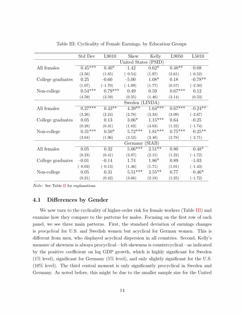
Table III: Cyclicality of Female Earnings, by Education Groups

Std Dev L9010 Skew Kelly L9050 L5010United States (PSID)

All females 0.45*** 0.40* –1.42 0.62* 0.48** –0.08(3.56) (1.85) (–0.54) (1.97) (2.61) (–0.52)

College graduates 0.25 –0.60 –5.00 1.08* 0.18 –0.78**(1.07) (–1.70) (–1.09) (1.77) (0.57) (–2.50)

Non-college 0.54*** 0.79*** 0.49 0.59 0.67*** 0.12(4.59) (3.59) (0.25) (1.46) (3.14) (0.53)

Sweden (LINDA)All females 0.27*** 0.43** 4.39** 1.64*** 0.67*** –0.24**

(3.26) (2.24) (2.76) (3.33) (3.09) (–2.67)College graduates 0.05 0.13 3.06* 1.15*** 0.64 –0.25

(0.28) (0.31) (1.82) (4.03) (1.22) (–1.74)Non-college 0.31*** 0.50* 5.72*** 1.81*** 0.75*** –0.25**

(3.04) (1.96) (3.52) (3.40) (2.78) (–2.71)Germany (SIAB)

All females 0.05 0.32 5.06*** 2.51** 0.80 –0.48*(0.23) (0.41) (3.87) (2.15) (1.22) (–1.72)

College graduates –0.01 –0.14 1.74 1.86* 0.89 –1.03(–0.03) (–0.13) (1.46) (1.71) (1.01) (–1.43)

Non-college 0.05 0.31 5.51*** 2.55** 0.77 –0.46*(0.21) (0.42) (3.66) (2.18) (1.25) (–1.72)

Note: See Table II for explanations.

4.1 Differences by Gender

We now turn to the cyclicality of higher-order risk for female workers (Table III) andexamine how they compare to the patterns for males. Focusing on the first row of eachpanel, we see three main patterns. First, the standard deviation of earnings changesis procyclical for U.S. and Swedish women but acyclical for German women. This isdifferent from men, who displayed acyclical dispersion in all countries. Second, Kelly’smeasure of skewness is always procyclical—left-skewness is countercyclical—as indicatedby the positive coefficient on log GDP growth, which is highly significant for Sweden(1% level), significant for Germany (5% level), and only slightly significant for the U.S.(10% level). The third central moment is only significantly procyclical in Sweden andGermany. As noted before, this might be due to the smaller sample size for the United

14

States.

Third, inspecting the top and bottom tails separately (last two columns), we observethe expected pattern of cyclicality, whenever the coefficient is significant. In particular,L9050 is procyclical and significant for the U.S. and Sweden, whereas the L5010 is coun-tercyclical and significant for Sweden and Germany.11 Thus, just as for the case of maleworkers, the behavior of the variance is driven by an asymmetric movement of the twotails rather than a uniform expansion of both tails. In our view, this finding reiteratesour earlier point that the variance is not an ideal statistic to focus on when it comes tomeasuring higher-order earnings risk over the business cycle. The case of U.S. womenis an excellent illustration of this point: the highly significant procyclicality of varianceis entirely driven by the upper tail. Finally, it is worth noting that the magnitudes ofthe fluctuations in both Kelly’s skewness and in the upper and lower tails separately aresomewhat attenuated for women compared with men.

4.2 Differences By Education Level

Economists have studied extensively how the average earnings and employment ofdifferent skill groups vary over the business cycle. We divide workers into two groups—college graduates and non-college workers—based on the highest education level theyhave acquired. Starting with males (Table II), in all three countries, both educationgroups display procyclical Kelly’s skewness that is statistically significant. In the UnitedStates and Sweden, the magnitude of cyclicality is quite a bit stronger for less educatedworkers—about three times stronger in both the U.S. and Sweden. In Germany, thedifference between the groups goes in the same direction but is quantitatively muchsmaller. Again, turning to standard deviation, there is not a very clear pattern in anycountry: variance is either acyclical or when it is pro-cyclical, the magnitude is small.

Turning to women in Table III, Sweden again emerges as the country with the clearestpatterns. Skewness is strongly procyclical for both education groups; the lower tail iscounter-cyclical for non-college and the upper tail is procyclical for non-college graduates.The variance for non-college graduates is also procyclical, although the magnitude is quitesmall. As discussed before, this happens because the top end of the shock distributioncollapses more than the expansion of the bottom end during recessions.

11It is somewhat surprising that women in the U.S. seem to face less downside risk as measured bythe L5010 differential compared with these two European countries.

15

In the U.S., the variance is more robustly procyclical for less educated women andacyclical for college graduates. In Germany, both non-college female workers and collegegraduates display acyclical dispersion of earnings changes. The overall pattern observedfor non-college workers resembles closely the estimates for all females, where a counter-cyclical lower tail (L5010) appears to be driving the volatility of earnings changes, whichdisplays significantly procyclical skewness. For more educated workers, only Kelly’s skew-ness is significantly procyclical at the 5% level, which resembles the result for Swedishwomen with college education. Again, the lack of significance for the U.S. estimates andthe German college-educated might be due to the lower share of employment amongwomen, especially in the earlier part of the sample, due to the relatively modest sam-ple size (in the U.S.) and low female college share (in the early part of the sample inGermany).

4.3 Differences Between Private- vs. Public-Sector Workers

One of the most pronounced differences between the economies of the United Statesand European countries, and Sweden in particular, is the size of the public employmentsector in the latter. Public sector jobs are often thought of as less risky, offering generousemployment protection and less volatile compensation, so it is interesting to ask if thisis borne out in the data. Because of data limitations for the U.S., we are able to conductthis analysis for Sweden and Germany only.

Our data set does not include a direct indicator of public sector employment. How-ever, some sectors in Sweden and Germany are dominated by public sector jobs (or,more broadly, by jobs funded by the public). So, we define a worker as working in thepublic sector, if he/she works in public administration, health care, or education in bothyears t and t + k (where k = 1, 5).12 The split between private/public employmentvaries substantially by gender: in Sweden about 23% of men work in the public sectorcompared with a whopping 63% for women (These figures have been relatively stableover the considered time period); in Germany a stable 10% of men work in the publicsector, while the share of women steadily increased from about 23% to about 25% overthe considered time period.

Table IV reports the cyclicality regressions separately for workers in private sectorversus public employment (by country). Interestingly, the results suggest stark differ-

12Historically most workers in these sectors were employed by the public; this is less true today.

16

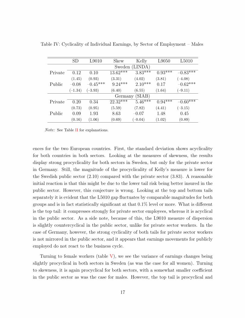
Table IV: Cyclicality of Individual Earnings, by Sector of Employment – Males

SD L9010 Skew Kelly L9050 L5010Sweden (LINDA)

Private 0.12 0.10 13.62*** 3.83*** 0.93*** –0.83***(1.45) (0.93) (3.31) (4.02) (3.81) (–4.08)

Public –0.08 –0.45*** 9.24*** 2.10*** 0.17 –0.62***(–1.34) (–3.93) (6.40) (6.55) (1.64) (–9.11)

Germany (SIAB)Private 0.20 0.34 22.32*** 5.46*** 0.94*** –0.60***

(0.73) (0.95) (5.59) (7.82) (4.41) (–3.15)Public 0.09 1.93 8.63 –0.07 1.48 0.45

(0.16) (1.06) (0.69) (–0.04) (1.02) (0.89)

Note: See Table II for explanations.

ences for the two European countries. First, the standard deviation shows acyclicalityfor both countries in both sectors. Looking at the measures of skewness, the resultsdisplay strong procyclicality for both sectors in Sweden, but only for the private sectorin Germany. Still, the magnitude of the procyclicality of Kelly’s measure is lower forthe Swedish public sector (2.10) compared with the private sector (3.83). A reasonableinitial reaction is that this might be due to the lower tail risk being better insured in thepublic sector. However, this conjecture is wrong. Looking at the top and bottom tailsseparately it is evident that the L5010 gap fluctuates by comparable magnitudes for bothgroups and is in fact statistically significant at that 0.1% level or more. What is differentis the top tail: it compresses strongly for private sector employees, whereas it is acyclicalin the public sector. As a side note, because of this, the L9010 measure of dispersionis slightly countercyclical in the public sector, unlike for private sector workers. In thecase of Germany, however, the strong cyclicality of both tails for private sector workersis not mirrored in the public sector, and it appears that earnings movements for publiclyemployed do not react to the business cycle.

Turning to female workers (table V), we see the variance of earnings changes beingslightly procyclical in both sectors in Sweden (as was the case for all women). Turningto skewness, it is again procyclical for both sectors, with a somewhat smaller coefficientin the public sector as was the case for males. However, the top tail is procyclical and

17

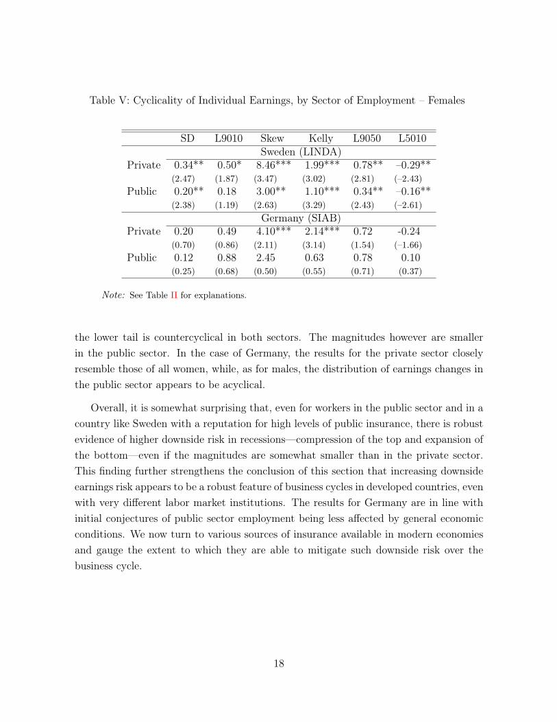
Table V: Cyclicality of Individual Earnings, by Sector of Employment – Females

SD L9010 Skew Kelly L9050 L5010Sweden (LINDA)

Private 0.34** 0.50* 8.46*** 1.99*** 0.78** –0.29**(2.47) (1.87) (3.47) (3.02) (2.81) (–2.43)

Public 0.20** 0.18 3.00** 1.10*** 0.34** –0.16**(2.38) (1.19) (2.63) (3.29) (2.43) (–2.61)

Germany (SIAB)Private 0.20 0.49 4.10*** 2.14*** 0.72 -0.24

(0.70) (0.86) (2.11) (3.14) (1.54) (–1.66)Public 0.12 0.88 2.45 0.63 0.78 0.10

(0.25) (0.68) (0.50) (0.55) (0.71) (0.37)

Note: See Table II for explanations.

the lower tail is countercyclical in both sectors. The magnitudes however are smallerin the public sector. In the case of Germany, the results for the private sector closelyresemble those of all women, while, as for males, the distribution of earnings changes inthe public sector appears to be acyclical.

Overall, it is somewhat surprising that, even for workers in the public sector and in acountry like Sweden with a reputation for high levels of public insurance, there is robustevidence of higher downside risk in recessions—compression of the top and expansion ofthe bottom—even if the magnitudes are somewhat smaller than in the private sector.This finding further strengthens the conclusion of this section that increasing downsideearnings risk appears to be a robust feature of business cycles in developed countries, evenwith very different labor market institutions. The results for Germany are in line withinitial conjectures of public sector employment being less affected by general economicconditions. We now turn to various sources of insurance available in modern economiesand gauge the extent to which they are able to mitigate such downside risk over thebusiness cycle.

18

5 Introducing Insurance

5.1 Within-Family Insurance

In the previous section, we have shown that higher-order moments drive individualearnings risk over the business cycle. While it is important to understand the underlyingnature of labor income risk and the systematic differences across groups, most of oursamples are composed by individuals in cohabitation.13 Assuming pooling of resourceswithin the household, the relevant income measure for many economic decisions is thejoint labor income in the household, not individual income. We therefore shift ourattention to joint labor earnings at the household level in order to shed light on the roleof informal insurance mechanisms within the household. As mentioned earlier, it is notpossible to link individuals in SIAB, so we rely on SOEP data instead.

Mixed Evidence of Within-Family Insurance

The first row of each panel in Table VI displays the cyclicality of each moment ofhousehold earnings changes. In order to get a feeling for the decrease (or increase) ofexposure to business cycle fluctuations, we compare these results to the correspondingmeasures for male earnings from Table II. Additional evidence comes from the graphicalanalysis of the dispersion, skewness, and the tails, of male earnings changes and householdearnings changes in Figures 3 and 4, respectively.

Addressing the fact that we use different data, the panel for Germany also displaysthe regression results for male earnings in the SOEP panel. The qualitative resultsusing SIAB and SOEP data broadly line up: standard deviation of earnings changes isacyclical, the lower tail is strongly countercyclical, and skewness—as measured by eitherthe third central moment or using Kelly’s measure—is procyclical. The upper tail is notsensitive to the cycle, whereas the lower tail responds strongly to aggregate fluctuations.This causes overall dispersion to be slightly countercyclical when measured by L9010,again driven by one of the tails alone. Overall, the measure of downside risk is robustacross data sets, while upside chances in booms seem to be slightly underestimated inSOEP.

Considering cyclicality of dispersion, the patterns and magnitudes for household earn-13Only 12% of our benchmark individual sample in the United States lives in a singe-person household,

for example.

19

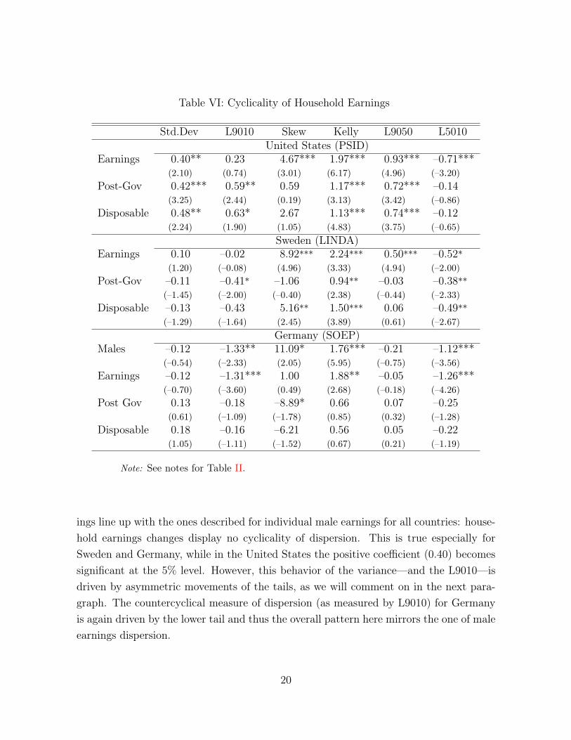
Table VI: Cyclicality of Household Earnings

Std.Dev L9010 Skew Kelly L9050 L5010United States (PSID)

Earnings 0.40** 0.23 4.67*** 1.97*** 0.93*** –0.71***(2.10) (0.74) (3.01) (6.17) (4.96) (–3.20)

Post-Gov 0.42*** 0.59** 0.59 1.17*** 0.72*** –0.14(3.25) (2.44) (0.19) (3.13) (3.42) (–0.86)

Disposable 0.48** 0.63* 2.67 1.13*** 0.74*** –0.12(2.24) (1.90) (1.05) (4.83) (3.75) (–0.65)

Sweden (LINDA)Earnings 0.10 –0.02 8.92*** 2.24*** 0.50*** –0.52*

(1.20) (–0.08) (4.96) (3.33) (4.94) (–2.00)Post-Gov –0.11 –0.41* –1.06 0.94** –0.03 –0.38**

(–1.45) (–2.00) (–0.40) (2.38) (–0.44) (–2.33)Disposable –0.13 –0.43 5.16** 1.50*** 0.06 –0.49**

(–1.29) (–1.64) (2.45) (3.89) (0.61) (–2.67)Germany (SOEP)

Males –0.12 –1.33** 11.09* 1.76*** –0.21 –1.12***(–0.54) (–2.33) (2.05) (5.95) (–0.75) (–3.56)

Earnings –0.12 –1.31*** 1.00 1.88** –0.05 –1.26***(–0.70) (–3.60) (0.49) (2.68) (–0.18) (–4.26)

Post Gov 0.13 –0.18 –8.89* 0.66 0.07 –0.25(0.61) (–1.09) (–1.78) (0.85) (0.32) (–1.28)

Disposable 0.18 –0.16 –6.21 0.56 0.05 –0.22(1.05) (–1.11) (–1.52) (0.67) (0.21) (–1.19)

Note: See notes for Table II.

ings line up with the ones described for individual male earnings for all countries: house-hold earnings changes display no cyclicality of dispersion. This is true especially forSweden and Germany, while in the United States the positive coefficient (0.40) becomessignificant at the 5% level. However, this behavior of the variance—and the L9010—isdriven by asymmetric movements of the tails, as we will comment on in the next para-graph. The countercyclical measure of dispersion (as measured by L9010) for Germanyis again driven by the lower tail and thus the overall pattern here mirrors the one of maleearnings dispersion.

20

The analysis of Kelly’s skewness—and the inspection of the tails—yields very inter-esting results when comparing the three countries. In Sweden, intra-family insuranceplays an important role in reducing downside risk over the business cycle as captured bya coefficient on Kelly’s skewness of about 2.2 (compared to 3.7 for male earnings). Thisdifference is mainly driven by the reaction of the lower tail being halved when movingfrom male earnings to household earnings. Repeating the illustrative calculation fromabove, this would imply a move from an upper tail to lower tail ratio of 50/50 in a typicalexpansion to 45/55 in a recession—much smaller compared to the change to 41/59 formale earnings.

Evidence of within-family insurance is weaker for the United States and Germany. Inboth economies, the results are slightly in favor of higher downside risk in recessions asmeasured by Kelly’s skewness in the case of gross household earnings than in the case ofindividual male earnings. The differences are rather small, though. Considering the tailsseparately for the two countries, reveals important differences. While the slightly strongerreaction of Kelly’s skewness is driven by higher procyclicality of upward movements inhousehold earnings as compared to male earnings in the United States, the opposite istrue in Germany. As for male earnings, the upper tail of earnings changes is not cyclicalin Germany – the lower tail widens more for household earnings.

We conclude that the responses of gross household earnings are heterogeneous acrosscountries, with Sweden being the only economy where the family plays a clear insurancerole against aggregate fluctuations. However, it is hard to extract further conclusions indisconnection to taxes and transfers payed and received by the household. In order toshed light on this issue, we move on to considering the role of social insurance policyover the business cycle.

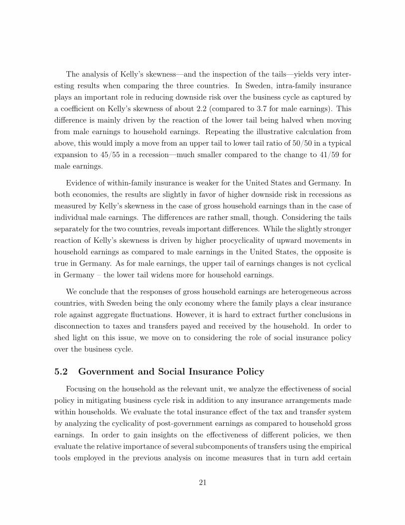
5.2 Government and Social Insurance Policy

Focusing on the household as the relevant unit, we analyze the effectiveness of socialpolicy in mitigating business cycle risk in addition to any insurance arrangements madewithin households. We evaluate the total insurance effect of the tax and transfer systemby analyzing the cyclicality of post-government earnings as compared to household grossearnings. In order to gain insights on the effectiveness of different policies, we thenevaluate the relative importance of several subcomponents of transfers using the empiricaltools employed in the previous analysis on income measures that in turn add certain

21

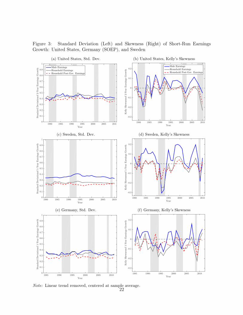
Figure 3: Standard Deviation (Left) and Skewness (Right) of Short-Run EarningsGrowth: United States, Germany (SOEP), and Sweden

(a) United States, Std. Dev.

Year

1980 1985 1990 1995 2000 2005 2010

Standard

Deviationof2-YearEarningsGrowth

0

0.1

0.2

0.3

0.4

0.5

0.6

0.7

0.8

0.9

1

Male Earnings

Household Earnings

Household Post-Gov. Earnings

(b) United States, Kelly’s Skewness

Year

1980 1985 1990 1995 2000 2005 2010

Kelly

Skew

nessof2-Y

earEarningsGrowth

-0.3

-0.2

-0.1

0

0.1

0.2Male Earnings

Household Earnings

Household Post-Gov. Earnings

(c) Sweden, Std. Dev.

Year

1980 1985 1990 1995 2000 2005 2010

Standard

Deviationof1-Y

earEarningsGrowth

0

0.1

0.2

0.3

0.4

0.5

0.6

0.7

0.8

0.9

1

(d) Sweden, Kelly’s Skewness

Year

1980 1985 1990 1995 2000 2005 2010

Kelly

Skew

nessof1-Y

earEarningsGrowth

-0.3

-0.2

-0.1

0

0.1

0.2

(e) Germany, Std. Dev.

Year

1985 1990 1995 2000 2005 2010

Standard

Deviationof1-Y

earEarningsGrowth

0

0.1

0.2

0.3

0.4

0.5

0.6

0.7

0.8

0.9

1

(f) Germany, Kelly’s Skewness

Year

1985 1990 1995 2000 2005 2010

Kelly

Skew

nessof1-Y

earEarningsGrowth

-0.3

-0.2

-0.1

0

0.1

0.2

Note: Linear trend removed, centered at sample average.22

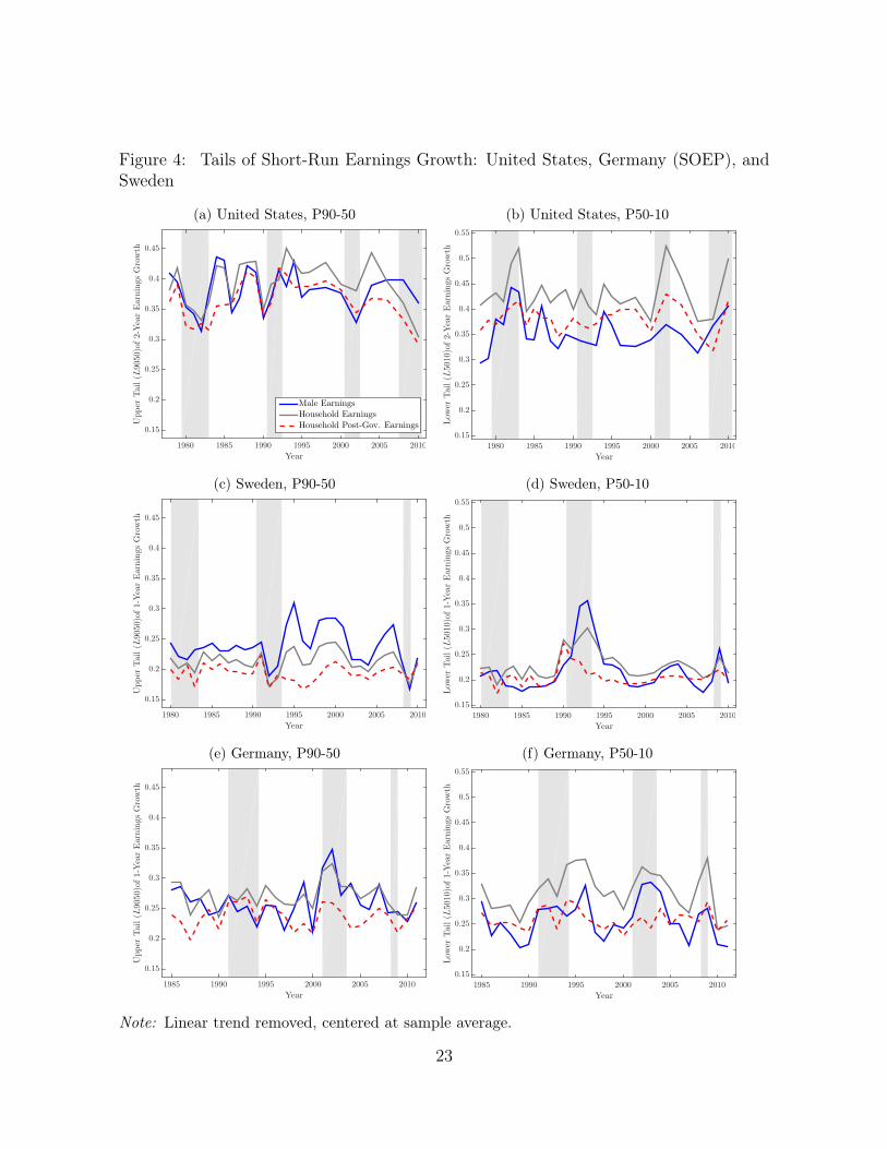
Figure 4: Tails of Short-Run Earnings Growth: United States, Germany (SOEP), andSweden

(a) United States, P90-50

Year1980 1985 1990 1995 2000 2005 2010

Upper

Tail(L

9050

)of2-YearEarnings

Growth

0.15

0.2

0.25

0.3

0.35

0.4

0.45

Male EarningsHousehold EarningsHousehold Post-Gov. Earnings

(b) United States, P50-10

Year1980 1985 1990 1995 2000 2005 2010

Low

erTail(L

5010

)of2-YearEarnings

Growth

0.15

0.2

0.25

0.3

0.35

0.4

0.45

0.5

0.55

(c) Sweden, P90-50

Year1980 1985 1990 1995 2000 2005 2010

Upper

Tail(L

9050

)of1-YearEarnings

Growth

0.15

0.2

0.25

0.3

0.35

0.4

0.45

(d) Sweden, P50-10

Year1980 1985 1990 1995 2000 2005 2010

Low

erTail(L

5010

)of1-YearEarnings

Growth

0.15

0.2

0.25

0.3

0.35

0.4

0.45

0.5

0.55

(e) Germany, P90-50

Year1985 1990 1995 2000 2005 2010

Upper

Tail(L

9050

)of1-YearEarnings

Growth

0.15

0.2

0.25

0.3

0.35

0.4

0.45

(f) Germany, P50-10

Year1985 1990 1995 2000 2005 2010

Low

erTail(L

5010

)of1-YearEarnings

Growth

0.15

0.2

0.25

0.3

0.35

0.4

0.45

0.5

0.55

Note: Linear trend removed, centered at sample average.

23

transfers to household gross earnings.

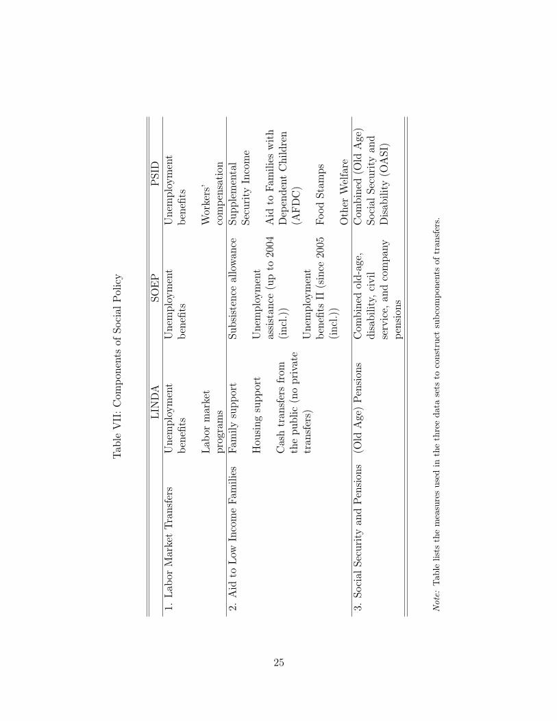
For the analysis of subcomponents, we consider three main groups of transfers thatare comparable across countries and for each country are consistently measured overtime. The groups are (1) labor-market-related policies, (2) aid to low-income families,and (3) “pensions,” and are listed in Table VII. Labor-market-related policies mainlyconsist of unemployment benefit payments—this component of social insurance policyis of particular importance for the mitigation of increased downside household earningsrisk in recessions, if the nature of downside risk is (temporary) job loss of household heador spouse.

The second component considered, “aid to low-income families,” consists of severalmeasures of social insurance policies specifically aimed at at-risk households. The rele-vance of this type of transfer can therefore be expected to matter most for low-incomehouseholds who have a higher likelihood of falling down to fulfilling ’at-risk’ criteria in thecourse of a recession. The third component, pension payments, is not directly connectedto business cycle considerations. It can still play a relevant role for household membersnear or at retirement age, who may take up pension payments instead of unemploymentpayments if they decide to leave the labor market upon job loss.

The Overall Effect of the Tax and Transfer System

We begin with a brief discussion on the overall effect of the government, comparing thecyclicality of pre- and post-government measures of household earnings listed in rows 1and 2 of Table VI. Again, Figures 3 and 4 visualize the findings. We find that social policyis an important source of insurance against aggregate fluctuations in all three economies,with very similar overall effects. Motivated by the considerations from above sections,we directly consider the reactions of the upper and lower tails of income changes. In allthree economies, downside risk is mitigated successfully by the tax and transfer system.In both the United States and Germany, the lower tail of post-government earningschanges is unresponsive to the business cycle—while significantly countercyclical for pre-government earnings. In Sweden, lower tail counter-cyclicality is dampened but stillstatistically significant (from a point estimate of –0.52 to –0.38).

Considering the cyclicality of the upper tail reveals differences between the countries.In Germany, it is unresponsive to the cycle for both pre-and post-government earnings.While both the U.S. and Sweden reveal procyclicality of L9050 of pre-government earn-

24

Tabl

eV

II:C

ompo

nent

sof

Soci

alPo

licy

LIN

DA

SOE

PP

SID

1.La

bor

Mar

ket

Tran

sfer

sU

nem

ploy

men

tbe

nefit

s

Labo

rm

arke

tpr

ogra

ms

Une

mpl

oym

ent

bene

fits

Une

mpl

oym

ent

bene

fits

Wor

kers

’co

mpe

nsat

ion

2.A

idto

Low

Inco

me

Fam

ilies

Fam

ilysu

ppor

t

Hou

sing

supp

ort

Cas

htr

ansf

ers

from

the

publ

ic(n

opr

ivat

etr

ansf

ers)

Subs

isten

ceal

low

ance

Une

mpl

oym

ent

assis

tanc

e(u

pto

2004

(incl

.))

Une

mpl

oym

ent

bene

fits

II(s

ince

2005

(incl

.))

Supp

lem

enta

lSe

curit

yIn

com

e

Aid

toFa

mili

esw

ithD

epen

dent

Chi

ldre

n(A

FDC

)

Food

Stam

ps

Oth

erW

elfa

re3.

Soci

alSe

curit

yan

dPe

nsio

ns(O

ldA

ge)

Pens

ions

Com

bine

dol

d-ag

e,di

sabi

lity,

civi

lse

rvic

e,an

dco

mpa

nype

nsio

ns

Com

bine

d(O

ldA

ge)

Soci

alSe

curit

yan

dD

isabi

lity

(OA

SI)

Note:

Tabl

elis

tsth

em

easu

res

used

inth

eth

ree

data

sets

toco

nstr

uct

subc

ompo

nent

sof

tran

sfer

s.

25

ings changes, the L9050 of post-government earnings changes is acyclical in Sweden, butstill procyclical in the United States. The different reactions of the tails translates intoprocyclical overall dispersion of post-government earnings changes in the U.S., and coun-tercyclical dispersion in Sweden. Summarizing the reaction of overall dispersion and tailsresults in procyclicality of Kelly’s skewness measure for both countries. This analysisreveals the importance of considering the tails separately.

To sum up, the analysis suggests that downside risk in recessions is mitigated bytaxes and transfers. In Sweden, an additional effect are lowered upside chances in ex-pansions. This lines up with considerations of Sweden as a country with a high degreeof redistribution.

The Role of Subcomponents of Social Policy

The measure of post-government earnings used so far lumps a lot of very differenttransfers received and taxes paid by households. While this measure is appropriate forassessing the overall effect of the tax and transfers system, it is not as well suited forunderstanding the success of different social policies that specifically aim at mitigatingdownside risk or that aims at aiding low-income families, who can be expected to beespecially vulnerable in recessionary periods. Therefore, we now consider different typesof transfers separately. The results of the cyclicality analysis are listed in Table VIII. Asfor for the estimates of total taxes and transfers, we compare the coefficients to the onesfrom the household gross earnings analysis in row 1 of Table VI. Recall that in order tobe in the year t base sample for the analysis, the lowest considered income measure ofa household needs to be above the income threshold for that year. This way, we ensurethat the sample is stable at the lower end of the distribution and results are not drivenby low-income households entering the sample for a certain type of transfer but are notin the sample when considering another.

The results in Table VIII show that labor market related transfers (which have un-employment benefits as the main component) are successful in mitigating downside riskin recessions in all three economies. This supports the consideration of an increasedincidence of unemployment in recessions. In the United States the cyclicality estimateof the lower tail of income changes is no longer statistically significant when consideringthese transfers (with the point estimate halved compared to household gross earnings).In the two European countries, the point estimates are cut by about a third. Consideringthe upper tail, in both the United States and Germany, there is no change when moving

26

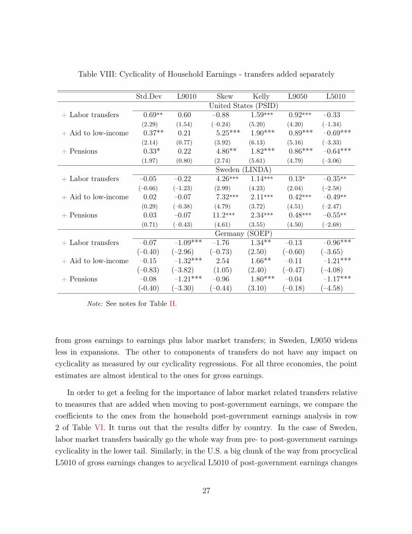
Table VIII: Cyclicality of Household Earnings - transfers added separately

Std.Dev L9010 Skew Kelly L9050 L5010United States (PSID)

+ Labor transfers 0.69** 0.60 –0.88 1.59*** 0.92*** –0.33(2.29) (1.54) (–0.24) (5.20) (4.20) (–1.34)

+ Aid to low-income 0.37** 0.21 5.25*** 1.90*** 0.89*** –0.69***(2.14) (0.77) (3.92) (6.13) (5.16) (–3.33)

+ Pensions 0.33* 0.22 4.86** 1.82*** 0.86*** –0.64***(1.97) (0.80) (2.74) (5.61) (4.79) (–3.06)

Sweden (LINDA)+ Labor transfers –0.05 –0.22 4.26*** 1.14*** 0.13* –0.35**

(–0.66) (–1.23) (2.99) (4.23) (2.04) (–2.58)+ Aid to low-income 0.02 –0.07 7.32*** 2.11*** 0.42*** –0.49**

(0.29) (–0.38) (4.79) (3.72) (4.51) (–2.47)+ Pensions 0.03 –0.07 11.2*** 2.34*** 0.48*** –0.55**

(0.71) (–0.43) (4.61) (3.55) (4.50) (–2.68)Germany (SOEP)

+ Labor transfers –0.07 –1.09*** –1.76 1.34** –0.13 –0.96***(–0.40) (–2.96) (–0.73) (2.50) (–0.60) (–3.65)

+ Aid to low-income –0.15 –1.32*** 2.54 1.66** –0.11 –1.21***(–0.83) (–3.82) (1.05) (2.40) (–0.47) (–4.08)

+ Pensions –0.08 –1.21*** –0.96 1.80*** –0.04 –1.17***(-0.40) (–3.30) (–0.44) (3.10) (–0.18) (–4.58)

Note: See notes for Table II.

from gross earnings to earnings plus labor market transfers; in Sweden, L9050 widensless in expansions. The other to components of transfers do not have any impact oncyclicality as measured by our cyclicality regressions. For all three economies, the pointestimates are almost identical to the ones for gross earnings.

In order to get a feeling for the importance of labor market related transfers relativeto measures that are added when moving to post-government earnings, we compare thecoefficients to the ones from the household post-government earnings analysis in row2 of Table VI. It turns out that the results differ by country. In the case of Sweden,labor market transfers basically go the whole way from pre- to post-government earningscyclicality in the lower tail. Similarly, in the U.S. a big chunk of the way from procyclicalL5010 of gross earnings changes to acyclical L5010 of post-government earnings changes

27

is accounted for by labor market transfers (the point estimate is statistically insignificantand thus supports the interpretation of acyclical income changes after considering labormarket transfers14). For Germany, other components not captured separately matter alot on top of labor market transfers for the mitigation of downside risk.

Moving to the upper tail, a big chunk on the way from procyclicality in gross earningschanges to acyclicality of L9050 of post-government earnings changes in the case ofSweden is already taken out from labor market transfers: the point estimate is only 0.13(and significant at the 10% level only) as compared to a highly (statistically) significantestimate of 0.5. In the case of the U.S., the upper tail is unaffected by this componentof social policy. Hence, the way to lower procyclicality of L9050 of post-governmentearnings changes is accounted for by other elements of the tax and transfer system.

While SIAB data set includes information on individuals and not on households,we do have information on unemployment benefits at the individual level. Table IXshows results for individual level regressions for male and female earnings separately,when unemployment benefits are excluded (rows 1 and 3) and included (2 and 4). Asexpected, including unemployment benefits reduces downside risk in recessions quitesignificantly for male workers. Workers who have a period of non-employment and hencezero earnings for a fraction of the year do not fall down to actually having zero income butreceive unemployment benefits during that period. For females, the insurance effect ofunemployment benefits goes in the expected direction as measured by reduced cyclicalityof the two skewness measures. Hence, these individual level results line up well with thehousehold level analysis conducted using SOEP data.

6 Welfare Analysis [To Be Completed]

15

In this section, we perform a simple quantitative exercise in order to gain someinsight into the welfare gains coming from the tax and transfer system. Suppose thathouseholds live in autarky, i.e., they are hand-to-mouth consumers. Further, we assumea CRRA per period utility function and, for each household, calculate the present value

14Again, this might partly be due to modest sample size.15In ongoing work, we are solving a full-fledged consumption-savings model to allow for some of the

the smoothing opportunities available to individuals and will perform a similar welfare analysis usingthis richer model. The draft will be updated to incorporate these results once they become becomeavailable.

28

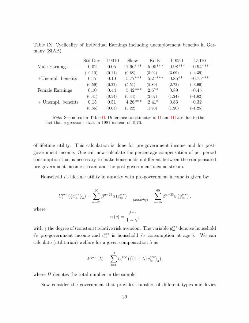
Table IX: Cyclicality of Individual Earnings including unemployment benefits in Ger-many (SIAB)

Std.Dev. L9010 Skew Kelly L9050 L5010Male Earnings –0.02 0.05 17.96*** 5.90*** 0.98*** –0.94***

(–0.10) (0.11) (9.68) (5.92) (3.09) (–4.39)+Unempl. benefits 0.17 0.10 15.77*** 5.27*** 0.85** –0.75***

(0.59) (0.22) (5.51) (5.80) (2.72) (–3.99)Female Earnings 0.10 0.44 5.42*** 2.67* 0.89 –0.45

(0.41) (0.54) (3.44) (2.02) (1.24) (–1.62)+ Unempl. benefits 0.15 0.51 4.26*** 2.41* 0.83 –0.32

(0.56) (0.63) (3.22) (1.90) (1.20) (–1.25)

Note: See notes for Table II. Difference to estimates in II and III are due to thefact that regressions start in 1981 instead of 1976.

of lifetime utility. This calculation is done for pre-government income and for post-government income. One can now calculate the percentage compensation of per-periodconsumption that is necessary to make households indifferent between the compensatedpre-government income stream and the post-government income stream.

Household i’s lifetime utility in autarky with pre-government income is given by:

Uprei ({cpreia }a) =

60X

a=25

�a�25u (cpreia ) =(autarky)

60X

a=25

�a�25u (ypreia ) ,

whereu (c) =

c1��

1� �,

with � the degree of (constant) relative risk aversion. The variable ypreia denotes householdi’s pre-government income and cpreia is household i’s consumption at age i. We cancalculate (utilitarian) welfare for a given compensation � as

W pre (�) ⌘HX

i=1

Uprei ({(1 + �) cpreia }a) ,

where H denotes the total number in the sample.

Now consider the government that provides transfers of different types and levies

29

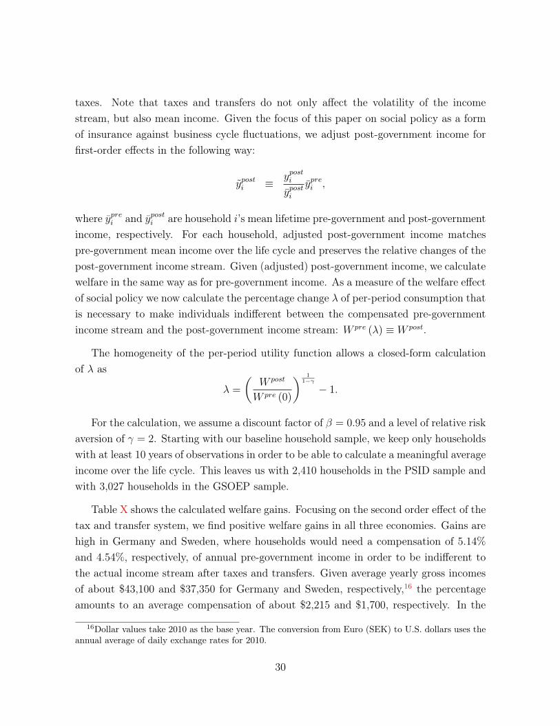
taxes. Note that taxes and transfers do not only affect the volatility of the incomestream, but also mean income. Given the focus of this paper on social policy as a formof insurance against business cycle fluctuations, we adjust post-government income forfirst-order effects in the following way:

yposti ⌘ yposti

yposti

yprei ,

where yprei and yposti are household i’s mean lifetime pre-government and post-governmentincome, respectively. For each household, adjusted post-government income matchespre-government mean income over the life cycle and preserves the relative changes of thepost-government income stream. Given (adjusted) post-government income, we calculatewelfare in the same way as for pre-government income. As a measure of the welfare effectof social policy we now calculate the percentage change � of per-period consumption thatis necessary to make individuals indifferent between the compensated pre-governmentincome stream and the post-government income stream: W pre (�) ⌘ W post.

The homogeneity of the per-period utility function allows a closed-form calculationof � as

� =

✓W post

W pre (0)

◆ 11��

� 1.

For the calculation, we assume a discount factor of � = 0.95 and a level of relative riskaversion of � = 2. Starting with our baseline household sample, we keep only householdswith at least 10 years of observations in order to be able to calculate a meaningful averageincome over the life cycle. This leaves us with 2,410 households in the PSID sample andwith 3,027 households in the GSOEP sample.

Table X shows the calculated welfare gains. Focusing on the second order effect of thetax and transfer system, we find positive welfare gains in all three economies. Gains arehigh in Germany and Sweden, where households would need a compensation of 5.14%and 4.54%, respectively, of annual pre-government income in order to be indifferent tothe actual income stream after taxes and transfers. Given average yearly gross incomesof about $43,100 and $37,350 for Germany and Sweden, respectively,16 the percentageamounts to an average compensation of about $2,215 and $1,700, respectively. In the

16Dollar values take 2010 as the base year. The conversion from Euro (SEK) to U.S. dollars uses theannual average of daily exchange rates for 2010.

30

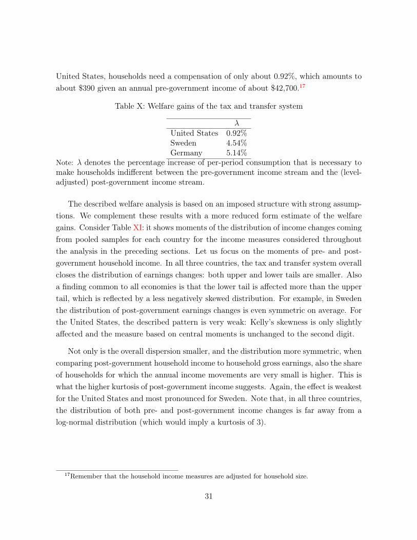
United States, households need a compensation of only about 0.92%, which amounts toabout $390 given an annual pre-government income of about $42,700.17

Table X: Welfare gains of the tax and transfer system

�United States 0.92%Sweden 4.54%Germany 5.14%

Note: � denotes the percentage increase of per-period consumption that is necessary tomake households indifferent between the pre-government income stream and the (level-adjusted) post-government income stream.

The described welfare analysis is based on an imposed structure with strong assump-tions. We complement these results with a more reduced form estimate of the welfaregains. Consider Table XI: it shows moments of the distribution of income changes comingfrom pooled samples for each country for the income measures considered throughoutthe analysis in the preceding sections. Let us focus on the moments of pre- and post-government household income. In all three countries, the tax and transfer system overallcloses the distribution of earnings changes: both upper and lower tails are smaller. Alsoa finding common to all economies is that the lower tail is affected more than the uppertail, which is reflected by a less negatively skewed distribution. For example, in Swedenthe distribution of post-government earnings changes is even symmetric on average. Forthe United States, the described pattern is very weak: Kelly’s skewness is only slightlyaffected and the measure based on central moments is unchanged to the second digit.

Not only is the overall dispersion smaller, and the distribution more symmetric, whencomparing post-government household income to household gross earnings, also the shareof households for which the annual income movements are very small is higher. This iswhat the higher kurtosis of post-government income suggests. Again, the effect is weakestfor the United States and most pronounced for Sweden. Note that, in all three countries,the distribution of both pre- and post-government income changes is far away from alog-normal distribution (which would imply a kurtosis of 3).

17Remember that the household income measures are adjusted for household size.

31

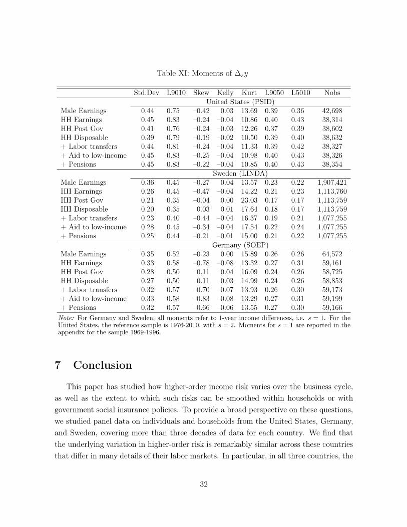
Table XI: Moments of �sy

Std.Dev L9010 Skew Kelly Kurt L9050 L5010 NobsUnited States (PSID)

Male Earnings 0.44 0.75 –0.42 0.03 13.69 0.39 0.36 42,698HH Earnings 0.45 0.83 –0.24 –0.04 10.86 0.40 0.43 38,314HH Post Gov 0.41 0.76 –0.24 –0.03 12.26 0.37 0.39 38,602HH Disposable 0.39 0.79 –0.19 –0.02 10.50 0.39 0.40 38,632+ Labor transfers 0.44 0.81 –0.24 –0.04 11.33 0.39 0.42 38,327+ Aid to low-income 0.45 0.83 –0.25 –0.04 10.98 0.40 0.43 38,326+ Pensions 0.45 0.83 –0.22 –0.04 10.85 0.40 0.43 38,354

Sweden (LINDA)Male Earnings 0.36 0.45 –0.27 0.04 13.57 0.23 0.22 1,907,421HH Earnings 0.26 0.45 –0.47 –0.04 14.22 0.21 0.23 1,113,760HH Post Gov 0.21 0.35 –0.04 0.00 23.03 0.17 0.17 1,113,759HH Disposable 0.20 0.35 0.03 0.01 17.64 0.18 0.17 1,113,759+ Labor transfers 0.23 0.40 –0.44 –0.04 16.37 0.19 0.21 1,077,255+ Aid to low-income 0.28 0.45 –0.34 –0.04 17.54 0.22 0.24 1,077,255+ Pensions 0.25 0.44 –0.21 –0.01 15.00 0.21 0.22 1,077,255

Germany (SOEP)Male Earnings 0.35 0.52 –0.23 0.00 15.89 0.26 0.26 64,572HH Earnings 0.33 0.58 –0.78 –0.08 13.32 0.27 0.31 59,161HH Post Gov 0.28 0.50 –0.11 –0.04 16.09 0.24 0.26 58,725HH Disposable 0.27 0.50 –0.11 –0.03 14.99 0.24 0.26 58,853+ Labor transfers 0.32 0.57 –0.70 –0.07 13.93 0.26 0.30 59,173+ Aid to low-income 0.33 0.58 –0.83 –0.08 13.29 0.27 0.31 59,199+ Pensions 0.32 0.57 –0.66 –0.06 13.55 0.27 0.30 59,166

Note: For Germany and Sweden, all moments refer to 1-year income differences, i.e. s = 1. For theUnited States, the reference sample is 1976-2010, with s = 2. Moments for s = 1 are reported in theappendix for the sample 1969-1996.

7 Conclusion

This paper has studied how higher-order income risk varies over the business cycle,as well as the extent to which such risks can be smoothed within households or withgovernment social insurance policies. To provide a broad perspective on these questions,we studied panel data on individuals and households from the United States, Germany,and Sweden, covering more than three decades of data for each country. We find thatthe underlying variation in higher-order risk is remarkably similar across these countriesthat differ in many details of their labor markets. In particular, in all three countries, the

32

variance of earnings shocks is almost entirely constant over the business cycle, whereasthe skewness of these shocks becomes much more negative in recessions. Governmentprovided insurance, in the form of unemployment insurance, welfare benefits, aid to lowincome households, and the like, plays a more important role reducing downside risk in allthree countries; the effectiveness is weakest in the United States, and most pronounced inGermany. For Sweden we find that insurance provided within households plays a similarrole. We calculate that the welfare benefits of social insurance policies for stabilizinghigher-order income risk over the business cycle range from 1% of annual consumptionfor the United States to 5% for Germany.

33

References

Daly, M., Hryshko, D. and Manovskii, I. (2014). Reconciling estimates of earningsprocesses in growth rates and levels, manuscript.

Dustmann, C., Ludsteck, J. and Schönberg, U. (2009). Revisiting the germanwage structure. Quarterly Journal of Economics, 124 (2), 843–881.

Fitzenberger, B., Osikominu, A. and Völter, R. (2006). Imputation rules to im-prove the education variable in the IAB employment subsample. Schmollers Jahrbuch.Zeitschrift für Wirtschafts- und Sozialwissenschaften, Jg. 126.

Guvenen, F., Ozkan, S. and Song, J. (2014). The Nature of Countercyclical IncomeRisk. Journal of Political Economy, 122 (3), 621–660.

Shin, D. and Solon, G. (2011). Trends in men’s earnings volatility: What does thepanel study of income dynamics show?,. Journal of Public Economics, 95 (7-8), 973–982.

Skedinger, P. (2007). The Design and Effects of Collectively Agreed Minimum Wages:Evidence from Sweden. Working Paper Series 700, Research Institute of IndustrialEconomics.

Storesletten, K., Telmer, C. I. and Yaron, A. (2004). Cyclical dynamics inidiosyncratic labor market risk. Journal of Political Economy, 112 (3), 695–717.

vom Berge, P., Burghardt, A. and Trenkle, S. (2013). Sample-of-Integrated-Labour-Market-Biographies Regional-File 1975-2010 (SIAB-R 7510). Tech. rep., Re-search Data Centre (FDZ) of the German Federal Employment Agency (BA) at theInstitute for Employment Research (IAB).

34

Appendices

A Data Appendix

This appendix briefly describes the variables used for each of the data sets and liststhe numbers of observations after the sample selection steps.

A.1 PSID

Variables

DEMOGRAPHIC AND SOCIOECONOMIC

Head and Relationship to Head. We identify current heads and spouses as thoseindividuals within the family unite with Sequence Number equal to 1 and 2, respectively.In the PSID, the man is labelled as the household head and the woman as his spouse.Only when the household is headed by a woman alone, she is considered the head. If thefamily is a split-off family from a sampled family, then a new head is selected.

Age. The age variable recorded in the PSID survey does not necessarily increase by 1from one year to the next. This may be perfectly correct, since the survey date changesevery year. For example, an individual can report being 20 years old in 1990, 20 in 1991,and 22 in 1992. We thus create a consistent age variable by taking the age reported inthe first year that the individual appears in the survey and add 1 to this variable in eachsubsequent year.

Education Level. In the PSID, the education variable is not reported every year andit is sometimes inconsistent. To deal with this problem, we use the highest educationlevel that an individual ever reports as the education variable for each year. Since oursample contains only individuals that are at least 25 years old, this procedure does notaffect our education variable in a major way.

INCOME AND HOURS

Individual Male Wages and Salaries. This is the variable used for individual in-come in the benchmark case. It is the answer to: How much did (Head) earn altogether

35

from wages or salaries in year t-1, that is, before anything was deducted for taxes orother things? This is the most consistent earnings variable over time reported in thePSID, as it has not suffered any redefinitions or change in subcomponents 18.

Individual Male Labor Earnings. Annual Total Labor Income includes all incomefrom wages and salaries, commissions, bonuses, overtime and the labor part of self-employment (farm and business income). Self-employment in PSID is split into assetand labor parts using a 50-50 rule in most cases. Because this last component has beeninconsistent over time,19 we subtract the labor part of business and farm income before1993.

Individual Female Labor Earnings. There is no corresponding Wages and Salaries

variable for spouses. We use Wife Total Labor Income and follow a similar procedureas in the case of heads.

Annual Hours. For heads and wives, it is defined as the sum of annual hours workedon main job, extra jobs and overtime. It is computed using usual hours of work per weektimes the number of actual weeks worked in the last year.

Pre-Government Household Labor Earnings. Head and wife labor earnings.

Post-Government Household Labor Earnings. Pre-government household earningsminus taxes plus public transfers, as defined below.

Taxes. The PSID reports own estimates for total taxes until 1991. For the remainingyears, we estimate taxes using TAXSIM.

Public Transfers. Transfers are considered at the family unit level, when possible. Wegroup social and welfare programs in three broad categories. Due to changes in thePSID design, the specific definition of each program is different every year. We give anoverview below and leave the specific replication details for the online Data Appendix.

Household Disposable Income. We construct this variable from Household TaxableIncome (Head’s and wife’s income from assets, earnings, and net profit from self-employment)minus taxes plus public transfers.

18See Shin and Solon (2011) for a comparison of PSID male earnings variables in inequality analyses.19In particular, total labor earnings included the labor parts of farm and business income up to the

1993 survey but not in subsequent waves.

36

TRANSFERS

We refer to Table VII in the main text for a description of the three groups ofprograms considered, as well as their subcomponents. In the PSID, obtaining an annualamount of each type of benefits is almost wave-specific. Every few survey years, the levelof aggregation within the family unit and across welfare programs is different for at leastone of our groups. To impose some common structure, we establish the following rules.

For survey years 1970–199320 and 2005–2011, the total annual amount of each pro-gram is reported for the head, spouse and others in the family unit. In occasions, theamount appears combined for several or all members.21 Because in those cases it is im-possible to identify separate recipiency of each member, we consider the benefit amountof the whole family. This is, we add up all available information for all family members,whether combined or separately reported.

In survey years 1994-2003, most benefits (except Food Stamps and OASDI) are re-ported separately for the head and the spouse only. The way amounts are reportedchanges as well. First, the reported amount ($X) received is asked. Second, the fre-quency of that amount ($X per year, per month, per week, etc) is specified. We convertall amounts to a common frequency by constructing a monthly amount $x using thesetime values. Finally, the head and spouse are asked during which months the benefitwas received. The final annual recipiency of transfers is then obtained multiplying $x

by the number of months this benefit was received. For Food Stamps and OASDI, wefollow the rules described for the other waves.

Detailed Sample Selection

We start with an initial sample of 584,392 SRC individuals interviewed between 1976and 2011. We then impose the next criteria every year. The number of individuals keptat each stage in the sample selection is listed in Table I. Previous to this selection process,we have cleaned the raw data and corrected duplicates and inconsistencies (for example,

20Our main sample refers to survey years 1977-2011, but complementary results are provided for theannual subsample of the PSID. This is, for 1970-1997. We drop the first two waves in all cases, sincebenefits such as OASDI, UI and WC are only reported for the family head; and benefits such as SSI arenot reported at all.

21This is always the case for Food Stamps.

37

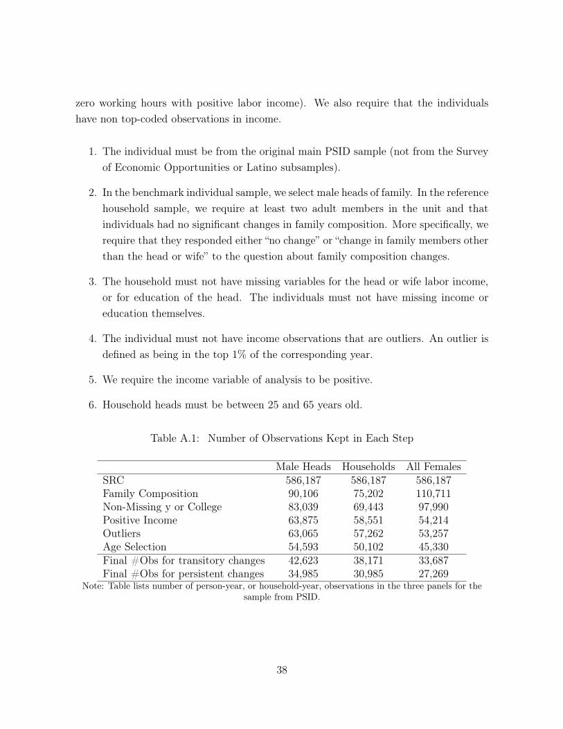
zero working hours with positive labor income). We also require that the individualshave non top-coded observations in income.

1. The individual must be from the original main PSID sample (not from the Surveyof Economic Opportunities or Latino subsamples).

2. In the benchmark individual sample, we select male heads of family. In the referencehousehold sample, we require at least two adult members in the unit and thatindividuals had no significant changes in family composition. More specifically, werequire that they responded either “no change” or “change in family members otherthan the head or wife” to the question about family composition changes.

3. The household must not have missing variables for the head or wife labor income,or for education of the head. The individuals must not have missing income oreducation themselves.

4. The individual must not have income observations that are outliers. An outlier isdefined as being in the top 1% of the corresponding year.

5. We require the income variable of analysis to be positive.

6. Household heads must be between 25 and 65 years old.

Table A.1: Number of Observations Kept in Each Step

Male Heads Households All FemalesSRC 586,187 586,187 586,187Family Composition 90,106 75,202 110,711Non-Missing y or College 83,039 69,443 97,990Positive Income 63,875 58,551 54,214Outliers 63,065 57,262 53,257Age Selection 54,593 50,102 45,330Final #Obs for transitory changes 42,623 38,171 33,687Final #Obs for persistent changes 34,985 30,985 27,269

Note: Table lists number of person-year, or household-year, observations in the three panels for thesample from PSID.

38

A.2 LINDA

Variables

Demographic and Socioeconomic

Head and Relationship to Head. LINDA is compiled from the Income Registerbased on filed tax reports and other registers. Statistics Sweden samples individuals andthen adds information for all family members, where family is defined for tax purposes.This implies that there is no information about ’head of households’ and insufficientinformation to determine relationships among family members. We therefore define thehead of a household as the sampled male, and define other adult members as spouses.

Age. As defined by Statistics Sweden

Education Level. LINDA contains information about eduction from 1991 and onwards.An individual is assigned “college” education if it has at least 3 years of university edu-cation.

Private / Public employment An individual is defined as as working in the publicsector, if he/she works in public administration, health care or education. Linda containsconsistent comparable information for the years 1991 and onwards. For the years 1991-92 the public sector employment is defined as those we use SNI90 codes 72000-72003,90000-93999 and >=96000. For 1993-2006 we use SNI92 codes 64110-64202, 73000-74110,75000-92000, 92500-92530 and >=96000. For 2007 we use SNI2007 codes 64110-64202,73000-74110, 75000-92000, 92500-92530 and >=96000.

Income

For the years 1985-2010 we use the measures suggested by Statistics Sweden to becomparable between years in LINDA. We construct comparable measure for the years1979-1984.

Individual labor income. Labor earnings consist of wages and salaries, the part ofbusiness income reported as labor income, and taxable compensation for sick leave andparental leave.

Pre-Government Household Labor Earnings. Defined as the sum of individuallabor income within the family.

39

Post-Government Household Labor Earnings. Post-government earnings is cal-culated as pre-government earnings minus taxes plus public transfers.

Household Disposable Income. Disposable income consists of the sum of factor incomeand minus taxes and plus public transfers.

Taxes. LINDA provides observations of total taxes paid by the individual. Since taxedpaid on capital income constitute a small part of total tax payments, and since we cannotseparate taxes on capital income from those on labor income, we assume that all taxesare labor income taxes.

Public Transfers. LINDA provides observations of total public transfers at the indi-vidual level (Statistics Sweden has individualized transfers given to families) and at thehousehold level. We also consider three subcategories of transfer as listed below.

Transfers

Transfers in subcategory 1 and 3 are individual level transfers. Transfers in subcate-gory 2 are family level transfers but have been individualized by Statistics Sweden. Foreach subcategory, we take all transfers received by all members of the households.

• HH-level transfers subcategory 1 (labor market transfers): sum of unemploymentbenefits received by all members of household.

• HH-level transfers subcategory 2 (family aid): sum of transfers to support familiesreceived by all members of household.

• HH-level transfers subcategory 3 (pensions): sum of old-age pensions received byall members of household.

Detailed Sample Selection

To be included in the individual sample the individual has to be sampled and between25 and 60 years old. A family is included in the household sample if the sampledindividual is a man between 25 and 60 years old and there are at least two membersaged 25-60 in the family.

40

A.3 SIAB

We use the scientific use file SIAB-R7510 provided by the Institute for EmploymentResearch (IAB). The SIAB data from which the scientific use file is constructed is a2% random sample of all individuals covered by a dataset called IEB. This data setis from four different sources, which can be identified in the data. For construction ofour sample we use earnings data stemming from BeH (employee history) and transferdata from LeH (benefit recipient history). Records in BeH are based on mandatory socialsecurity notifications from employers and hence cover individuals working in employmentsubject to social security, which excludes civil servants, students and self-employed. Anew spell starts whenever there is a new notification, which happens when either a newemployment relationship changes, an ongoing contract is changed, or with the start ofa calendar year. BeH covers all workers subject to social security contributions, whichexcludes civil servants, self-employed and students. For details on the data set see vomBerge et al. (2013).

Variables

Demographic and Socioeconomic

Head and Relationship to Head. SIAB does not contain information on households.We use only individual level data.

Age. Birth year is reported consistently in SIAB data.

Education Level. Each individual spell in SIAB contains information on the highestdegree of formal education as reported by the employer. In order to construct a consistentmeasure of education we apply imputation rules proposed by Fitzenberger et al. (2006).

Private / Public employment An individual is defined as as working in the publicsector, if he/she works in public administration, health care or education. SIAB containsconsistent comparable information for all years of the sample. We use the classificationWZ93 as provided in the data, which aggregates 3 digit codes of the original WZ93classification into 14 categories. The industry of an employer is registered once a yearand assigned to the worker spells of that year. This implies that for some individualspells there is no information on the industry. For each year a worker is assigned theindustry from the longest spell in that year. We classify as public employment those in

41

sectors 13 (3-digit WZ93 801–804, 851-853: Education, social and health-care facilities)and 14 (751–753, 990: public administration, social security).

Income

Individual labor income. We calculate annual earnings as the sum of total earningfrom all valid spells for each individual. As marginal employment spells were not reportedbefore 1999, we drop marginal employment in the years where they are reported to obtaina time consistent measure. For the same reason we drop spells with reported averagedaily wage rate below the highest marginal employment threshold in the sample period,which is 14.15 Euros (in 2003 Euros). There are two drawbacks in the available data:structural break of the wage measure in 1984 and top-coding.

Structural break in wage measure Since 1984 the reported average daily wage ratefrom an employment spell includes one-time payments. We correct for this structuralbreak following a procedure based on Dustmann et al. (2009): we rank individuals from1976 to 1983 into 50 quintiles of the annual full-time wage distributions. Then we fitlocally weighted regressions of the wage growth rate from 1982-1983 on the quintiles in1983 and the same for 1983-1984. We then define as the correction factor the differencebetween the quintile-specific smoothed value of wage growth between 1984 and 1983. Theunderlying assumption is that wage growth should be higher from 1983-1984 because thewage measure includes one-time payments. In order to control for overall wage growthdifferences we subtract the average of the correction factor of the second to 20th quintiles.The resulting percentile-specific correction factor is then applied to wages in 1976-1983.

Imputation of top-coded wages Before aggregating earnings from all spells we cor-rect full-time wage spells for the top-coding. We therefore follow Daly et al. (2014)and fit a Pareto tail to the cross-sectional wage distribution. The Pareto distribution isestimated separately for each year by age-group and sex. We define seven age groups:25-29,30-34,...,55-60. As starting point for the Pareto we choose the 60th percentile ofthe subgroup-specific distribution. As in Daly et al. (2014), we draw one random numberby individual which we then apply to the annual specific distributions when assigning awage to the top-coded workers. We apply the imputation method to the annual distri-bution of average full-time wages and hence an individual can be below the cutoff limitif, e.g., from two full-time spells in a year only one is top-coded. We therefore define astop-coding limit the annual specific limit minus 3 DM (1995 DM) as in ?.

42

Transfers

In SIAB we observe consistently over time unemployment benefits at the individuallevel.

Detailed Sample Selection

To be included in the sample the individual has to be between 25 and 60 years oldand earn a gross income above 520*0.5*minimum wage. We drop all workers which haveat least one spell reported in East Germany.

SOEP

Variables

Demographic and Socioeconomic

Head and Relationship to Head. For each individual in the sample, SOEP reportsthe relationship to the head of household in any given wave. Whenever there is a non-couple household, i.e., no spouse is reported, the reported head is classified as head.Whenever we observe a couple household and the reported head is a male we keep this;when the reported head is a female and the reported spouse is a male, we reclassify themale to be head and the female to be spouse.

Age. The age is measured by subtracting year of birth from the current year.

Education Level. The education variable used categorizes the obtained maximumeducation level by ISCED 1997. An individual with category 6 is assigned “college”education, an individual with categories 1-5 is assigned “non-college”. Category 6 includesa degree obtained from university, from technical college, from a university abroad, and aPhD. An individual still in school (category 0) is assigned a missing. For a small numberof individuals the described procedure yields inconsistencies in the sense that for someyear t the assignment is “college” and some later year t+s the assignment is “non-college”;in these cases we assign “college” to the later year.

Income and Hours

Individual labor income. Labor earnings are calculated from individual labor incomecomponents and includes income from first job, secondary job, 13th and 14th salary,

43

christmas bonus, holiday bonus, profit sharing. For consistency with the PSID measurewe assign 50% of income from self-employment to labor income.

Household level labor income. Defined as the sum of individual labor income ofhead and spouse.

Annual Hours. SOEP measures the average actual weekly hours worked and the num-bers of months an individual worked. From these measures SOEP provides a constructedmeasure of annual hours worked of an individual.

Pre-Government Household Labor Earnings. Head and spouse labor earnings.

Post-Government Household Labor Earnings. Pre-government household earn-ings minus taxes plus public transfers, as defined below.

Taxes. SOEP provides estimates of total taxes at the household level.

Public Transfers. Transfers are considered at the family unit level and at the indi-vidual level. We group social and welfare programs in three broad categories as listedbelow.

Household Disposable Income. We construct this variable from Household Taxable In-come (Head’s and wife’s income from assets, earnings, and net profit from self-employment)minus taxes plus public transfers. SOEP provides a measure of household asset flows,which is calculated as income from renting minus operating costs, plus dividend income.

Transfers

Transfers are partly observed at the individual level and partly at the household level.For each subcategory, we take all transfers received by all members of the households.

• HH-level transfers : we use transfers received by all individual household membersin order to calculate measures that are consistent over time. For each individual,total transfers are the sum of the following components: old-age pensions, widow’spensions, maternity benefit, student grants, unemployment benefits, subsistenceallowance, unemployment assistance (up to 2004); at the hh-level we measure re-ceived child allowances and the total unemployment benefits II received by allhousehold members (since 2005 replacing unemployment assistance).

44

• HH-level transfers subcategory 1 (labor market transfers): sum of unemploymentbenefits received by all members of household.

• HH-level transfers subcategory 2 (family aid): sum of subsistence allowance of allmembers, + sum of unemployment assistance received by all members (up to 2004),+ hh-level measure of unemployment benefits II (since 2005).

• HH-level transfers subcategory 3 (pensions): sum of old-age pensions received byall members of household.

Sample Selection

In order to be in the initial sample for a year, the individual or household head must bebetween ages 25 and 60 and live in West Germany. In order to have a consistent sample,we drop the immigrant subsample and the high income subsample. This gives initialsample sizes of 87,582 individual-year observations for the male sample, 76,249 individual-year observations for the female sample, and 76,051 household-year observations for thehousehold sample. The sample selection then follows the steps listed below for eachsample. All cross-sectional statistics are calculated using appropriate cross-sectionalindividual or household weights, respectively.

1. drop if no info on education or if no degree obtained yet

2. drop if currently working in military

3. drop if no info on income

4. drop if no info on hours worked

5. keep if income > 0 and hours > 520

6. drop if in highest percentile (sample outliers)

7. drop if below 520*0.5*minimum wage, where minimum wage is set to be 6€ inyear 2000 Euros

8. for transitory change measure: keep if in sample in t and t-1

9. for permanent change measure: keep if in sample in t and t-5

45

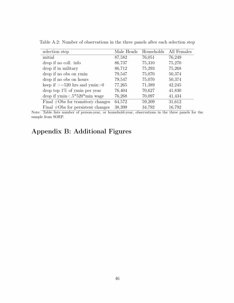
Table A.2: Number of observations in the three panels after each selection step

selection step Male Heads Households All Femalesinitial 87,582 76,051 76,249drop if no coll. info 86,737 75,310 75,270drop if in military 86,712 75,293 75,268drop if no obs on ymin 79,547 75,070 50,374drop if no obs on hours 79,547 75,070 50,374keep if >=520 hrs and ymin>0 77,265 71,389 42,245drop top 1% of ymin per year 76,404 70,627 41,830drop if ymin<.5*520*min wage 76,268 70,097 41,434Final #Obs for transitory changes 64,572 59,209 31,612Final #Obs for persistent changes 38,399 34,792 16,792

Note: Table lists number of person-year, or household-year, observations in the three panels for thesample from SOEP.

Appendix B: Additional Figures

46

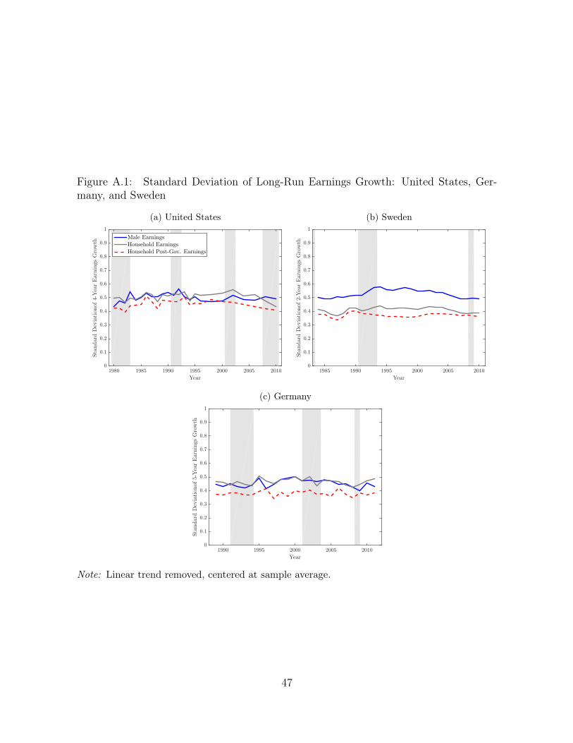
Figure A.1: Standard Deviation of Long-Run Earnings Growth: United States, Ger-many, and Sweden

(a) United States

Year

1980 1985 1990 1995 2000 2005 2010

Standard

Deviationof4-YearEarningsGrowth

0

0.1

0.2

0.3

0.4

0.5

0.6

0.7

0.8

0.9

1

Male Earnings

Household Earnings

Household Post-Gov. Earnings

(b) Sweden

Year

1985 1990 1995 2000 2005 2010

Standard

Deviationof2-YearEarningsGrowth

0

0.1

0.2

0.3

0.4

0.5

0.6

0.7

0.8

0.9

1

(c) Germany

Year

1990 1995 2000 2005 2010

Standard

Deviationof5-YearEarningsGrowth

0

0.1

0.2

0.3

0.4

0.5

0.6

0.7

0.8

0.9

1

Note: Linear trend removed, centered at sample average.

47

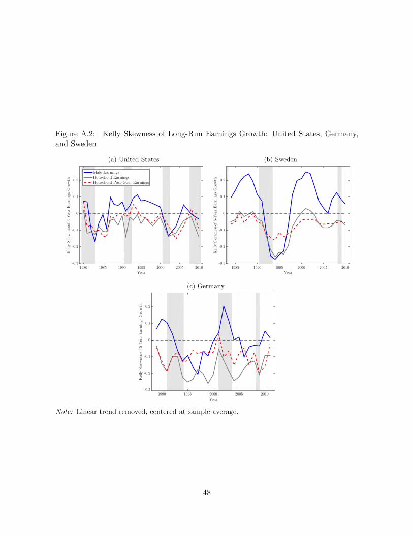
Figure A.2: Kelly Skewness of Long-Run Earnings Growth: United States, Germany,and Sweden

(a) United States

Year

1980 1985 1990 1995 2000 2005 2010

Kelly

Skew

nessof4-Y

earEarningsGrowth

-0.3

-0.2

-0.1

0

0.1

0.2

Male Earnings

Household Earnings

Household Post-Gov. Earnings

(b) Sweden

Year

1985 1990 1995 2000 2005 2010

Kelly

Skew

nessof5-Y

earEarningsGrowth

-0.3

-0.2

-0.1

0

0.1

0.2

(c) Germany

Year

1990 1995 2000 2005 2010

Kelly

Skew

nessof5-Y

earEarningsGrowth

-0.3

-0.2

-0.1

0

0.1

0.2

Note: Linear trend removed, centered at sample average.

48

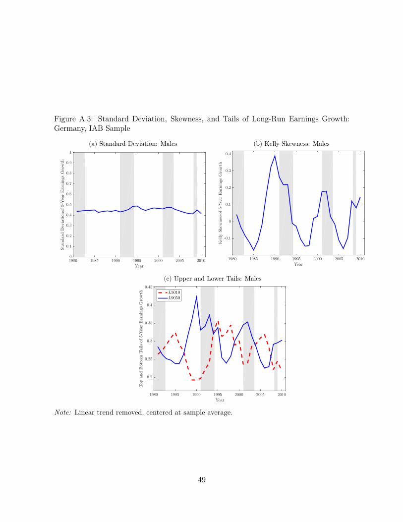
Figure A.3: Standard Deviation, Skewness, and Tails of Long-Run Earnings Growth:Germany, IAB Sample

(a) Standard Deviation: Males

Year

1980 1985 1990 1995 2000 2005 2010

Standard

Deviationof5-YearEarningsGrowth

0

0.1

0.2

0.3

0.4

0.5

0.6

0.7

0.8

0.9

1

(b) Kelly Skewness: Males

Year

1980 1985 1990 1995 2000 2005 2010

Kelly

Skew

nessof5-YearEarningsGrowth

-0.1

0

0.1

0.2

0.3

0.4

(c) Upper and Lower Tails: Males

Year

1980 1985 1990 1995 2000 2005 2010

TopandBottom

Tailsof5-YearEarningsGrowth

0.2

0.25

0.3

0.35

0.4

0.45

L5010

L9050

Note: Linear trend removed, centered at sample average.

49