Higher-Order Co-occurrences for Exploratory PointPattern Analysis

and Decision Tree Clustering on Spatial Data

D.G. Leibovici∗,a, L. Bastinb, M. Jacksona

aCentre for Geospatial Sciences, University of Nottingham, UKbSchool of Engineering and Applied Science, Aston University, UK

Abstract

Analyzing geographical patterns by collocating events, objects or their attributes

has a long history in surveillance and monitoring, and is particularly applied in

environmental contexts, such as ecology or epidemiology. The identification of

patterns or structures at some scales can be addressed using spatial statistics,

particularly marked point processes methodologies. Classification and regres-

sion trees are also related to this goal of finding “patterns” by deducing the

hierarchy of influence of variables on a dependent outcome. Such variable se-

lection methods have been applied to spatial data, but, often without explic-

itly acknowledging the spatial dependence. Many methods routinely used in

exploratory point pattern analysis are second-order statistics, used in a uni-

variate context, though there is also a wide literature on modelling methods

for multivariate point pattern processes. This paper proposes an exploratory

approach for multivariate spatial data using higher-order statistics built from

co-occurrences of events or marks given by the point processes. A spatial en-

tropy measure, derived from these multinomial distributions of co-occurrences

at a given order, constitutes the basis of the proposed exploratory methods.

Key words: spatio-temporal data, spatial statistics, co-occurrences,

multivariate data, marked point process, regression trees, spatial entropy, R

∗Corresponding authorEmail addresses: didier.leibovici@nottingham.ac.uk (D.G. Leibovici),

l.bastin@aston.ac.uk (L. Bastin), Mike.Jackson@nottingham.ac.uk (M. Jackson)

Preprint submitted to Elsevier June 16, 2010

programming

1. Introduction

Geographical pattern in experimental datasets is frequently investigated by

collocating events, objects or their attributes, particularly when the aim is to

monitor the environment, as in ecology or epidemiology (Wagner and Fortin,

2005; Bastin et al., 2007b). In spatial statistics, this is often associated with

marked point processes (Diggle, 2003; Schabenberger and Gotway, 2004). In or-

der to identify patterns, or at least to establish the existence of certain structures

at some scales, spatial dependence functions, e.g. cross-K functions, may be

plotted against distance. These functions can be tested for significance against

the functions produced by complete randomness or other hypothetical processes,

or against the results of random labelling. Typically, a set of Monte Carlo reali-

sations is used to generate a “null hypothesis” confidence envelope, encompass-

ing, for example, 95% of the results from the random or hypothesised process

(Diggle et al., 2007; Schlather and Diggle, 2004; Lotwick and Silverman, 1982).

For a review on recent developments in modelling multivariate spatial processes,

see also Baddeley et al. (2006). Classification/Decision/Regression trees such

as CART (Breiman et al., 1984), ID3 (Quinlan, 1986), and PEGASE (Phipps,

1981), are also related to the goal of finding “patterns” by selecting and priori-

tising variables according to their hierarchy of influence on a dependent outcome

or on a specific statistic. Often these methods have been applied, without any

adaptation, to spatial data, though some authors propose specific modifications

to account for spatial dependence (Bel et al., 2009; Li and Claramunt, 2006).

Recently, the potential for analyzing co-occurrences of spatial events at

higher order has been explored in Leibovici et al. (2008) and Leibovici (2010), in

the context of correspondence analysis, the CAkOO method. This exploratory

method breaks down the χ2 statistic for the lack of independence between the

co-occurrences of the categorical variables in a similar way to that in which a

principal component analysis breaks down the total variance (or inertia). One

2

can call this independence a spatial independence since this is done using spa-

tial contingencies: the co-occurrences. Multinomial distributions of spatial co-

occurrences demand the consideration of other statistics or metrics which are

linked to spatial patterns of multi-type marked event processes and multivariate

point processes. As exploratory functions for structure and scale, entropy mea-

sures derived from these multinomial distributions of co-occurrences at a given

order are considered.

We present here two approaches using spatial co-occurrence and the entropy

measure. The first exploratory method considers all pre-selected variables and

covariates of the events and analyses the plot of the observed spatial entropies

from co-occurrences of order k (a SOOk curve), along with its null hypothe-

sis envelope (obtained here via Monte-Carlo simulation according to random

labelling). The second method (in an approach similar to PEGASE) looks at

the best clustering which can be obtained by hierarchical selection of covariates

(SelSOOk method). SelSOOk can then provide an optimized selection of covari-

ates to be used in a SOOk analysis or in a CAkOO analysis. CAkOO, SOOk

and SelSOOk have been implemented in R (R Development Core Team, 2007)

using packages for managing spatial data (see Bivand (2008) for a comprehen-

sive state of the art) and in particular spatstat (Baddeley and Turner, 2005)

and PTAk (Leibovici, 2010).

There are various contexts in environmental monitoring where the detec-

tion of changes in a complex system may involve the study of multi-covariate

patterns, i.e. studying interactions, rather than marginal changes. These con-

texts include vegetation succession and the spread of disease, and two example

datasets from these application domains are used to illustrate the methods de-

rived for this purpose. The examples, which are discussed in detail below, are

taken from an epidemiological study in England, and a vegetation biodiversity

survey in Greece.

3

2. Environmental dataset examples

For the purposes of this paper, the techniques outlined above and devel-

oped in further sections were tested on two point datasets with multivariate

attributes. Both were projected to local National Grids for the areas from

which they were collected, with distance units in meters. In both datasets,

some elements of spatial structure had been identified in previous studies, using

well-tested techniques. This meant that they were useful benchmarks on which

to test these novel exploratory methods.

2.1. Epidemiological dataset

The first dataset is from an epidemiological study, which investigated the dis-

tributions of meticillin-resistant Staphylococcus aureus (MRSA) and its antibiotic-

sensitive counterpart, (SA) in and around a British city (Bastin et al., 2007b).

The variates recorded, i.e. the marks (labels), consisted of information on pa-

tient gender, age group, the date on which the disease was diagnosed, and

the nature of the disease (MRSA or SA). The spatial locations of the point

records are derived from postcode centroids, so that each patient is sited at the

population-weighted center of the postcode polygon in which they reside. In the

Bastin et al. (2007b) study, the data was subjected to kernel density filtering

and spatial scan techniques. When compared to “null” Monte Carlo simulations

which echoed the underlying population density and age structure, significant

spatio-temporal clusters of MRSA were discovered using these techniques.

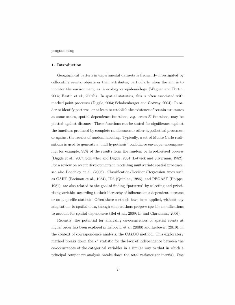
This data has a naturally patchy spatial structure, (see Figure 1), because

of the underlying heterogeneity in population density, and the “snapping” of

a patient’s location to the postcode centroid, rather than their exact address,

could potentially cause problems for studies where it is necessary to calculate

real inter-point distances. However, for a random labelling approach this is less

of an issue, since all sets of labelled points are subject to the same artificially-

imposed granularity. For this reason, a random labelling approach (MRSA/SA)

was applied in Bastin et al. (2007b) to investigate whether MRSA cases tended

to cluster together more strongly than SA cases; this was found to be the case

4

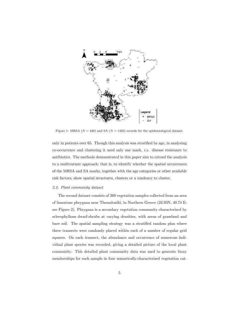
Figure 1: MRSA (N = 428) and SA (N = 1450) records for the epidemiological dataset.

only in patients over 65. Though this analysis was stratified by age, in analysing

co-occurrence and clustering it used only one mark, i.e. disease resistance to

antibiotics. The methods demonstrated in this paper aim to extend the analysis

to a multivariate approach; that is, to identify whether the spatial occurrences

of the MRSA and SA marks, together with the age categories or other available

risk factors, show spatial structures, clusters or a tendency to cluster.

2.2. Plant community dataset

The second dataset consists of 269 vegetation samples collected from an area

of limestone phrygana near Thessaloniki, in Northern Greece (22.93N, 40.74 E:

see Figure 2). Phrygana is a secondary vegetation community characterized by

sclerophyllous dwarf-shrubs at varying densities, with areas of grassland and

bare soil. The spatial sampling strategy was a stratified random plan where

three transects were randomly placed within each of a number of regular grid

squares. On each transect, the abundance and occurrence of numerous indi-

vidual plant species was recorded, giving a detailed picture of the local plant

community. This detailed plant community data was used to generate fuzzy

memberships for each sample in four numerically-characterised vegetation cat-

5

egories, identified using DECORANA (see Table 1) (Bastin et al., 2007a).

Tclu1 “Open Grassland”Tclu2 “Dense Cistus/Quercus scrub”Tclu3 “Medium Cistus scrub”Tclu4 “Dense Quercus/Pyrus/Pinus”

Table 1: Community characterization of the fuzzy clustering membership.

Although the defined communities represent complex assemblages of species,

for simplicity’s sake in Table 1 they have been named after their dominant,

or defining, components. These assemblages tend to mix and grade into one

another across the landscape, resulting in mixed memberships at some points,

and “pure” samples at others.

Figure 2: Locations of sampling points within the vegetation dataset

The aim of the original study was to see whether unknown sites could be

easily classified into complex vegetation categories from simpler metrics which

are more easily and cheaply measured, and which can often be assessed from

remotely-sensed imagery. This can be crucial for monitoring purposes in avoid-

6

ing long and expensive surveys. For this reason, a number of simpler variables

were collected, as follows: patchiness of the transect (Patch) (i.e., variation

in cover type); Texture of the transect (Tex) (i.e. total changes in vegetation

height along its length); slope (Slope) and aspect (Aspect) of the sample site;

% of area covered by open grassland/ground (open), low shrub (low), high

shrub (high), tree cover (tree), and mixed shrub and tree cover (s&t) (bold

face acronyms will be used in the analysis section). In the analysis described

here, the focus is on identifying the best “simple” variables for predicting and

describing the spatial distribution of the cluster membership values that repre-

sent the richer multi-species dataset.

3. From 2nd-order to kth-order analysis

The events which are recorded spatially for a particular study in a geographic-

related discipline, e.g. ecology, epidemiology or crime studies, are usually con-

sidered in spatial statistics as being associated with a point process, that is

“a stochastic mechanism generating a countable set of events”(Diggle, 2003;

Bivand, 2008); locations of events correspond to points in the studied spatial

domain. A spatial point pattern is thus seen as a realization of the point process

X in a bounded domain W , leading to a finite number of observations, each

x ⊂ X ∩W . When attribute values are attached to each location or each event,

one gets a marked point process: that is, a realization of a point process and a

marking process. Each point x has a mark m and the observation is xm. The

challenge for point pattern analysis is to assess the associations of marks for the

same process or for different processes, and the degree to which they depend

on other covariates. The cross-K function can be used, but becomes limited

when studying multivariate systems as the number of comparisons of pairs can

increase dramatically.

3.1. Extending 2nd-order statistics

Practical questions often deal directly with higher-order statistical issues.

For example, an ecologist may be interested to know whether, within a given

7

landscape, the association of two specific plant species occurs more often on one

specific soil type. A more exploratory approach would be to assess whether there

is a particular structuring of plant species and soil types with habitat types. For

this purpose, quadrat count distributions associated with sampling designs have

been used intensively in landscape ecology but suffer from the MAUP (Mod-

ifiable Area Unit Problem) issue, as discussed in Wagner and Fortin (2005).

Quadrat count statistics are also often first-order summaries, targeting, for ex-

ample, a richness index. The principle of quadrat counts shows, nonetheless,

that the focus is on co-occurrences of events and the distribution of these co-

occurrences.

Classical estimators of statistics based on moments are in fact expressed by

co-occurrences. For example, for an inhomogeneous marked point process, a

symmetric cross-type Ripley’s K statistic can be expressed:

K̂Slm(d) =

1

|W |∑

{xl,xm}⊂X∩W

1(d(xl, xm) ≤ d)

λ(xl)λ(xm)(1)

where |W | is the area of the window W over which the marked point process

X is evaluated; l and m are the two marks of interest; xl and xm are any two

observed points, respectively with marks l and m, of the pattern associated

with X; the sum is over pairs of points, sampled from X with marks l and m,

and found in W ; d is the distance of co-occurrence and the function 1() is the

indicator function (its value is 1 if the evaluated expression is true, 0 otherwise);

and λ(xm) is the intensity of the process at point xm. The above formula is

adapted from Baddeley et al. (2000) without edge correction.

A simple extension of Ripley’s K Equation (1) to higher orders gives, here

choosing the order k = 3:

K̂Smop(d) = (2)

1

|W |∑

{xm,xo,xp}⊂X∩W

1(dP (xm, xo, xp) ≤ d)

λ(xm)λ(xo)λ(xp)

where dP is the maximum distance between any pair of the evaluated points (the

distance used in the examples is the Euclidean distance). The capital subscript

8

P refers to this Pairwise consideration of distance, and is distinct from the

lower-case subscript p used to denote a mark. When the indicator function

1(dP (xm, xo, xp) ≤ d) equals 1, a co-occurrence of order 3 between marks m,

o, and p for the given points is counted. If the denominator is constant the

numerator of the statistic counts the co-occurrences between these marks. The

extension for any order k > 3 is a straightforward extension of Equation (2). The

statistic of Equation (2) accounts for lower-order moments as well. For example,

if, in Equation (2) the marks m and o are the same, then, the numerator of the

statistic accounts for 2rd-order co-occurrences as well as 3th-order of the marks

m, and p. To be purely of kth-order a constraint must be added, as follows: for

equal marks, the corresponding points have to be different.

4. Multiple Co-occurrences for Spatial Entropy

If, conditionally to the marks, the process is assumed to be homogeneous,

then the intensities can be estimated by λ̂(xl) = λ̂l = nl/|W |, where nl is

the number of points with mark l. In this case, equations such as (1) and (2)

correspond to a ratio representing lack of independence, as in the χ2 measure

of independence. For example, the 3rd-order statistic can be written:

1/|W |∑

xl,xm,xp⊂X∩W

1(dP (xl, xm, xp) ≤ d)

λ(xl)λ(xm)λ(xp)= (3)

1/|W |∑{} 1(dP (xl, xm, xp) ≤ d)

(nl/|W |)(nm/|W |)(np/|W |)=

1/|W |nlmp

n...

n...

n3

(nl/|W |)(nm/|W |)(np/|W |)/n3=

plmp/collpcoll

plpmpp

= Olmp/Elmp

where Olmp is the observed probability of co-occurrences of three points with

marks l, m, and p; Elmp is the estimate of this probability under the hypothesis

of complete independence of the collocating events. These probabilities have

to be understood as normalized to the unit surface (because of |W |). Other

notations and necessary derivations are: nlmp =∑{} 1(dP (xl, xm, xp) ≤ d)

9

is the number of collocations of the marks l, m and p; n... =∑

l,m,p nlmp is

the total number of 3rd-order collocations; pl = (1/|W |)nl/n is the probabil-

ity of finding a point with mark l in W, n being the total number of points.;

pcoll = (1/|W |)n.../n3 is the probability of a triple of marks to collocate in W

and plmp/coll = nlmp/n... is the probability of finding the marks l, m and p

conditionally to have three co-occurrent points in W.

Without making any homogeneity assumption on the sub-processes1, Lei-

bovici et al. (2008) and Leibovici (2010) describe the analysis of a contingency

table of co-occurrences, such as the multiway table nlmp of Equation (3), using

correspondence analysis for multiway table: the CAkOO method (Correspon-

dence Analysis of k cO-Occurrences). CAkOO analyses spatial independence

but does not directly test or quantify the existence of a pattern, nor does it test

at which “scale” it exists (one distance d of collocation is chosen in advance).

A multiscale analysis can nonetheless be done by adding a scale dimension in

the multiway table (Leibovici et al., 2007; Leibovici and Jackson, 2008).

Multivariate co-occurrence distributions, derived from one or different pro-

cesses, describe the spatial structure or organization of the events and the inter-

actions between or within the processes. Here are some examples of multivariate

co-occurrence distribution choices using the plant community dataset; they are

hypothetical and we used a very different analysis strategy with this dataset

(see further with the SelSOOk analysis):

• A multivariate co-occurrence of interest would be the association between

the clustering of the species communities (Tclu1-Tclu4), and the variables

Patch (recoded into 3 categories) and Slope (recoded into 2 categories).

Note that for this example, the point processes for all the variables are the

same, so that one has a multivariate multivariable marking process on a

single point process. For a given distance of co-occurrence, the collocation

counts for the three variables are ntps, for collocations of points with a

1as in the rest of the paper.

10

cluster membership t, a patchiness category p and a slope category s,

resulting in a table of dimension 4× 3× 2.

• One can look at nt1t2t3 , where only the structure of collocations of the

variable identifying species cluster membership is of interest (only one

process is in fact analyzed), giving a table of collocation counts of dimen-

sion 4× 4× 4.

• Alternatively, one can look at nijk where i, j and k are either a species

cluster membership, a patchiness category and a slope category, so build-

ing a symmetric table of dimensions (4 + 3 + 2)× (4 + 3 + 2)× (4 + 3 + 2),

where all collocation patterns of order 3 are recorded.

In order to summarize the “meaningfulness” of a pattern, we need some in-

dex which can numerically compare structured to random configurations, i.e.

a measure of “spatial entropy”. Shannon entropy, originating in information

theory, has commonly been used for this purpose on spatial data consisting of

raw category distributions, and has also been adapted to take into account the

adjacency counts of categories (O’Neill et al., 1988). Higher-order co-occurrence

can be seen as an extension of adjacency. Using the multivariate co-occurrence

distribution, one can assess the spatial structure and dependence of one (or

more) multi-type marked process(es), using as spatial entropy the index:

HSu(Coo, d) = −1/ log(NCoo)∑coo

pcoo,d log(pcoo,d) (4)

where Coo is a multivariate co-occurrence of attributes considered from one or

more multi-type marked point processes, generating the collocation counts with

the multi-index coo, and thus the distribution pcoo,d. The collocation is for a

chosen distance value d and a chosen order k - in most of the examples, k = 3.

The multi-index coo has k positions with values for each position depending on

the marks involved (see the above examples). NCoo is the number of multi-

indexes coo, that is the number of cells of the multiway table, so that the term

log(NCoo) corresponds to a normalization relative to the entropy of a uniform

11

distribution. HSu stands for spatial entropy relative to uniformity: the Shannon

entropy is usually termed H and the subscript S is for spatial, u to express the

ratio to uniformity.

A univariate index can also be derived, by only considering as interesting

values in Coo the co-occurrences of each category with itself, that is the ones

corresponding to the hyper-diagonal of the co-occurrence table, a k entries table,

e.g. niii for an order k = 3:

HsSu(CooI , d) = −1/log(I)

I∑i

ps(i),d log(ps(i),d) (5)

with a given order of co-occurrences, defined by the length of the multi-index s()

and where I is the number of categories. The self multi-index s() expresses the

fact that the observed probabilities are computed only using the hyper-diagonal

of the counts of co-occurrences, e.g. with co-occurrences of order 3:

ps(i),d = niii/∑i

niii (6)

The self spatial entropy, also normalized to uniformity, HsSu, then measures

the spatial pattern according to clustering of occurrences of the same categories

(derived from attribute values) of the points. As for the classical Shannon

entropy, low values of HSu and/or HsSu means the existence of some structure in

the distribution, which in this case implies a spatial structure of the marks. Since

the spatial measures are normalized, as they approach 1, so the distribution of

co-occurrences gets closer to the uniform distribution.

5. Examples of SOOk and SelSOOk analyses

For the SOOk method, plotting the spatial entropy against distance of co-

occurrence allows the study of potential patterns at different scales. Evidence

of low entropy, due to spatial configuration of the marks when compared to the

same point process with different marks, can be obtained from Monte Carlo test

simulations using random labelling.

12

5.1. Lansing woods dataset

Before looking at the example datasets described at the beginning of this

paper, we looked at a classical point pattern data existing in the literature and

in the R-package spatstat (Baddeley and Turner, 2005): the Lansing data,

consisting of 2251 trees in a 924 x 924 feet plot rescaled to a unit square. The

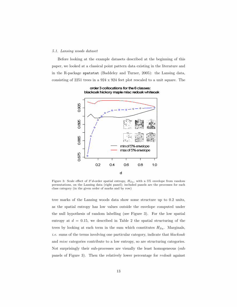
Figure 3: Scale effect of 3rd-order spatial entropy, HSu, with a 5% envelope from randompermutations, on the Lansing data (right panel); included panels are the processes for eachclass category (in the given order of marks and by row)

tree marks of the Lansing woods data show some structure up to 0.2 units,

as the spatial entropy has low values outside the envelope computed under

the null hypothesis of random labelling (see Figure 3). For the low spatial

entropy at d = 0.15, we described in Table 2 the spatial structuring of the

trees by looking at each term in the sum which constitutes HSu. Marginals,

i.e. sums of the terms involving one particular category, indicate that blackoak

and misc categories contribute to a low entropy, so are structuring categories.

Not surprisingly their sub-processes are visually the least homogeneous (sub

panels of Figure 3). Then the relatively lower percentage for redoak against

13

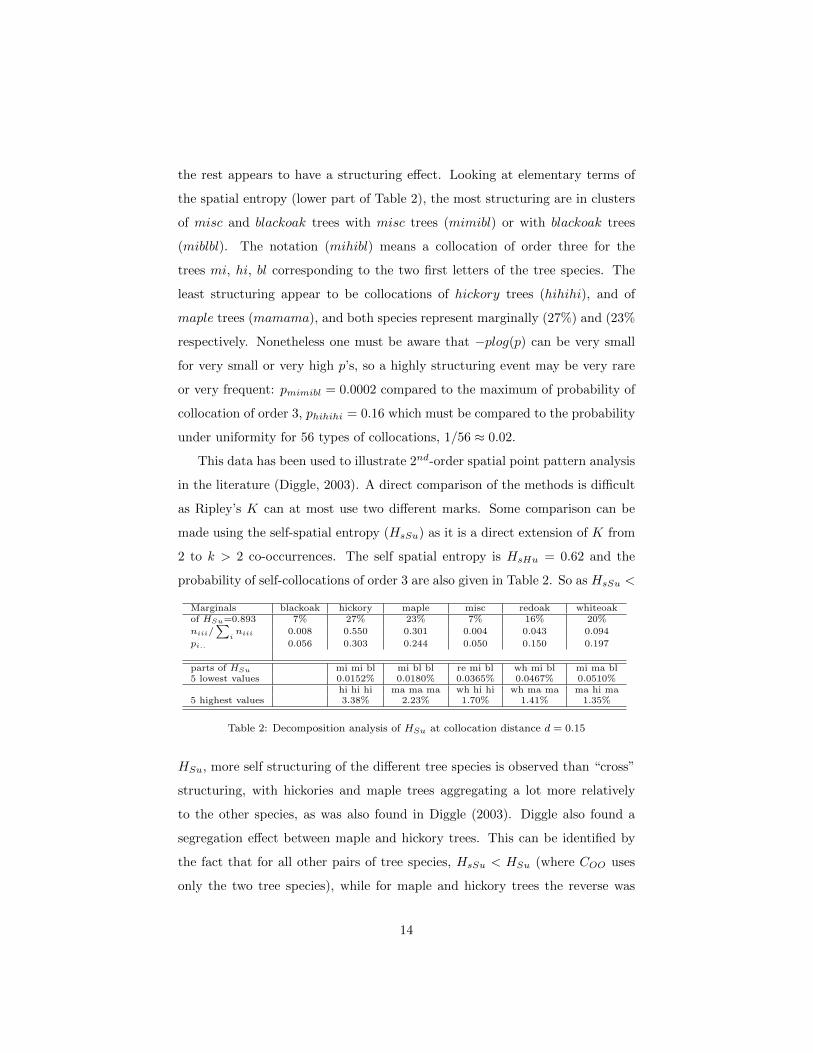
the rest appears to have a structuring effect. Looking at elementary terms of

the spatial entropy (lower part of Table 2), the most structuring are in clusters

of misc and blackoak trees with misc trees (mimibl) or with blackoak trees

(miblbl). The notation (mihibl) means a collocation of order three for the

trees mi, hi, bl corresponding to the two first letters of the tree species. The

least structuring appear to be collocations of hickory trees (hihihi), and of

maple trees (mamama), and both species represent marginally (27%) and (23%

respectively. Nonetheless one must be aware that −plog(p) can be very small

for very small or very high p’s, so a highly structuring event may be very rare

or very frequent: pmimibl = 0.0002 compared to the maximum of probability of

collocation of order 3, phihihi = 0.16 which must be compared to the probability

under uniformity for 56 types of collocations, 1/56 ≈ 0.02.

This data has been used to illustrate 2nd-order spatial point pattern analysis

in the literature (Diggle, 2003). A direct comparison of the methods is difficult

as Ripley’s K can at most use two different marks. Some comparison can be

made using the self-spatial entropy (HsSu) as it is a direct extension of K from

2 to k > 2 co-occurrences. The self spatial entropy is HsHu = 0.62 and the

probability of self-collocations of order 3 are also given in Table 2. So as HsSu <

Marginals blackoak hickory maple misc redoak whiteoakof HSu=0.893 7% 27% 23% 7% 16% 20%

niii/∑

iniii 0.008 0.550 0.301 0.004 0.043 0.094

pi.. 0.056 0.303 0.244 0.050 0.150 0.197

parts of HSu mi mi bl mi bl bl re mi bl wh mi bl mi ma bl5 lowest values 0.0152% 0.0180% 0.0365% 0.0467% 0.0510%

hi hi hi ma ma ma wh hi hi wh ma ma ma hi ma5 highest values 3.38% 2.23% 1.70% 1.41% 1.35%

Table 2: Decomposition analysis of HSu at collocation distance d = 0.15

HSu, more self structuring of the different tree species is observed than “cross”

structuring, with hickories and maple trees aggregating a lot more relatively

to the other species, as was also found in Diggle (2003). Diggle also found a

segregation effect between maple and hickory trees. This can be identified by

the fact that for all other pairs of tree species, HsSu < HSu (where COO uses

only the two tree species), while for maple and hickory trees the reverse was

14

observed, expressing rarer cross-collocations.

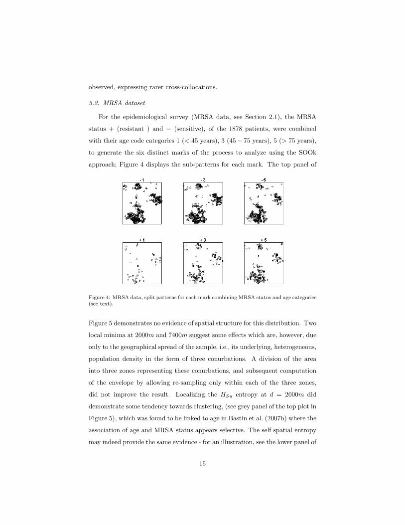
5.2. MRSA dataset

For the epidemiological survey (MRSA data, see Section 2.1), the MRSA

status + (resistant ) and − (sensitive), of the 1878 patients, were combined

with their age code categories 1 (< 45 years), 3 (45− 75 years), 5 (> 75 years),

to generate the six distinct marks of the process to analyze using the SOOk

approach; Figure 4 displays the sub-patterns for each mark. The top panel of

Figure 4: MRSA data, split patterns for each mark combining MRSA status and age categories(see text).

Figure 5 demonstrates no evidence of spatial structure for this distribution. Two

local minima at 2000m and 7400m suggest some effects which are, however, due

only to the geographical spread of the sample, i.e., its underlying, heterogeneous,

population density in the form of three conurbations. A division of the area

into three zones representing these conurbations, and subsequent computation

of the envelope by allowing re-sampling only within each of the three zones,

did not improve the result. Localizing the HSu entropy at d = 2000m did

demonstrate some tendency towards clustering, (see grey panel of the top plot in

Figure 5), which was found to be linked to age in Bastin et al. (2007b) where the

association of age and MRSA status appears selective. The self spatial entropy

may indeed provide the same evidence - for an illustration, see the lower panel of

15

Figure 5, where self collocations of order 3 for age categories are also displayed

(at d = 2000m) for the sub-processes defined by the MRSA status. There is

clearly a structure of age within patients with MRSA as compared to a nearly

uniform distribution for the SA status, and this is confirmed by the histograms

shown at d = 2000m (bottom of Figure 5). One benefit of the method presented

here is that all ’age’ marks could be considered simultaneously, and their relative

structuring effects compared, while in the original study, three separate analyses

were required to identify the same phenomenon - one for each age group.

5.3. With the plant community dataset

The spatial entropy measure based on co-occurrences can also be used for

regression tree clustering. An approach similar to PEGASE (Phipps, 1981) is

taken here. SelSOOk can be performed either with no target variable or with a

target variable.

With no target variable, a hierarchy of variables is looked for according to

the best spatial structure obtained at each level of the hierarchy. A spatial

structure is defined by the spatial pattern of the marking of the points using a

given series of variables. At each level of the hierarchy, the set of all preceding

variables in the hierarchy constitutes the series of variables to be used. The

optimization for best spatial structure is obtained by looking for the minimum

joint spatial entropy2 of the set of variables: at the ith step, the variable X(i)

minimizing HSu(X(1), X(2), ..., X(i)) is added into the hierarchy.

With a target variable, the best hierarchy of variables is obtained as in a

stepwise regression. Note that here the focus is not on the best spatial struc-

turing set of variables but the best at explaining the spatial structure of the

target variable. At each step, the set of variables acts like regressors and the

conditional entropy2 is the criterion to minimize. Joint and conditional en-

tropies were derived from Equation (4) and using classical entropy formula2

2The joint entropy of two variables X and Y is the H(X,Y ), the entropy of joint proba-bility distribution; the conditional entropy, H(Y |X) is the expectation of the entropies on theconditional probabilities given the values of X; the joint entropy and the conditional entropyare linked by: H(Y |X) = H(X,Y )−H(X), see for example Reza (1994).

16

Figure 5: Scale effect of 3rd-order spatial entropy on the MRSA data: (top panel) on thecombined age and MRSA status 6 classes with a 5% envelope from random permutations,the grey panel displays a localized HSu at d = 2000m split in three classes; (bottom panel)comparison of the self-spatial entropy for the 3 age classes for the whole process and thesub processes for each MRSA status; included panels are the age histograms for each MRSAcategory (by row): histograms based on self-collocation counts (at d = 2000m) on the left andsimple histograms of the categories on the right.

17

(the normalization to uniformity cannot be used for the conditional entropy).

For simplicity of implementation the criterion minimized for the ith variable was:

HS(Y,X(1), X(2), ..., X(i−1)|X(i)) instead ofHS(Y |X(1), X(2), ..., X(i−1), X(i)). These

two optimization are very similar, as:

H(Y |X(1), X(2)) = H(Y,X(1)|X(2))−H(X(1)|X(2)) (7)

so minimizing the left hand of equation (for best 2nd variable) would also ensure

that the additional variable X(2) is the least “correlated” with the previous

variable X(1).

True tree clustering proceeds by splitting the data at each stage where a

new clustering variable is selected, leading to classes which are not necessarily

built with the same set of variables. Only the procedure without split has

been implemented here. Note that there is still a tree, and that this tree is

symmetrical: at each level, the nodes are split with the same variable and the

optimization is done per level, not per node (on each split sample) as in a true

tree clustering.

The plant community dataset (see Section 2.2), containing 269 point sam-

ples with attributes representing vegetation metrics, was used to illustrate the

alternative SelSOOk analysis. On Figure 6 the analyses are: (i) a tree clustering

of the vegetation indices as they capture the spatial structure (ii) and then as

they explain the spatial structure of the crisp clustering membership variable

Tclu(variable coded from allocating each sample to the cluster in which it has

highest membership). For simplicity, the vegetation indices were here coded as

binary: high and low values based on their histograms. The sequence of the best

four variables for joint spatial entropy is identical (tree, low, Patch, open) at

all distances of collocation. However, the fifth best variable depends on colloca-

tion distance: in most cases it is s&t but at 5 meters (the finest spatial scale)

it is high.

As expected, the joint spatial entropy increases as variables are added to

describe the structure of the data (top panel of Figure 6). Tree cover (tree)

is persistent at all scale and well in front of the other variables. The sequence

18

Figure 6: Scale effect with 3rd-order SelSOOk tree clustering of the plant community dataset;[Top] subsequent values HSu(X(1), X(2), ..., X(i)) where i = 1, ..., 5 is the best ith selected vari-able. [Bottom] same with the conditional entropy HS(Y,X(1), X(2), ..., X(i−1)|X(i)), whereY is the crisp classes from transect data clustering (top panel), and X(i)’s are the vegetationcoded indices.

19

of the variables is persistent through the change in scale factor (the distance of

collocation). Note that the relief variables, Slope and Aspect, do not play an

important part here.

On the other hand, the other SelSOOk analysis (in the lower panel of Fig-

ure 6), showed some effect from Slope but as fifth variable in the hierarchy and

only at 25 and 30 meters of collocation. The decrease of the conditional en-

tropy as the hierarchy of variables expands to explain the crisp clustering target

variable was also expected from the classical formula of entropy. Explaining the

crisp clustering coming from transect data (Tclu), one must notice the change of

hierarchy as the scale factor changes, with an approximate consistency for three

scale divisions: micro (5m-10m), medium (15m-30m), larger (35m-65m). The

variables selected in the sequences show some differences to the ones obtained

for (i), as follows:

• 05-10 meters: high, tree, s&t, open, Tex

• 10-10 meters: high, tree, open, s&t, Tex

• 15-20 meters: open, low, s&t, Tex, high

• 25-30 meters: open, low, s&t, Tex, Slope

• 35-65 meters: s&t, tree, open, Tex, high.

At finer scale high shrubs comes in first to explain the plant community clus-

tering variable, but was not in the first four variables for the analysis in (i).

Still comparing to the results for (i), Patchiness disappears from the best four

variables, as not linked to the spatial distribution of the plant community clus-

tering variable. These results are consistent with the observed patterns, and

give valuable further insights. When the four clusters are referenced back to

the vegetation communities they represent (Table 1), it can be seen that the

“Open” (Tclu1) and “Medium Shrub” (Tclu3) clusters are widely and evenly

spaced across the landscape, reflecting the way in which variables s&t and open

move up the hierarchy with increasing spatial lag. In contrast, dense shrub and

20

tree communities are characteristically highly spatially clustered, leading to the

predominance of variables high and tree at the smallest landscape grain. Tex,

which represents the local variability in structure at each sample point, is impor-

tant at every spatial scale but never dominates as the driver in spatial structure.

6. Discussions and Further issues

Considering multiple co-occurrences’ distributions for one or more point pro-

cesses, a generic spatial entropy index was derived to analyze dependence in

marked point processes at different scales (collocation distances). SOOk and

SelSOOk methods were developed, which;

• analyze higher-order statistics towards clustered occurrences versus uni-

formity;

• generate tree classification of variables with an optimization either looking

for minimum joint spatial entropy, or minimum conditional spatial entropy

when a target or dependent variable is to be explained.

The choice of the order of co-occurrence plays an important role. Other experi-

ments suggest that, for one categorical variable (one set of marks), increasing the

order increases the discriminatory power offered by the spatial entropy index,

between spatially-structured data versus less structured or randomly-patterned

data (Leibovici, 2009). In these experiments, we used the k-values 2, 3 and 4.

Obviously, increasing the order puts into question the necessary size of the stud-

ied sample for the underlying estimation of high order moments. A downside

of the methods is about interpreting the results, particularly with the SOOk

method where detecting a tendency to clustering with a pooled index does not

inform which profiles (out of all the categories involved) are responsible for this

effect. The CAkOO method may help in this description. To assess the sig-

nificance of the observed scale effects for the spatial entropy index, we checked

one of the possible hypotheses, namely the random labelling hypothesis which

is conditional on the locations. When different point processes express differ-

ent marks, one might also wish to test their independence (van Lieshout and

21

Baddeley, 1999). Note that here, as HSu and HsSu are relative to uniformity

of the co-occurrences, they measure something to be related to the spatial in-

dependence of the sub-processes. However, a theoretical variance is needed to

be able to provide an confidence envelope under this hypothesis. We did not

investigate the usual independence test, considered in point pattern analysis,

of complete spatial randomness where the hypothesis is that the point pattern

comes from an homogeneous Poisson process. This hypothesis will, however, be

a useful starting point for further investigations..

A Ripley’s K extension, (see Equation 2), has been introduced here pri-

marily as a conceptual link with established point pattern analysis, but as a

generalization of a well known statistic in point pattern analysis, this exten-

sion is interesting in its own right; future work on its stochastic properties,

and specifically its sampling distribution, will create opportunities for further

hypothesis testing. The relationship to existing methods of exploratory point

pattern analysis has been partially investigated in this paper by comparison to

previous analyses, and some specific benefits and limitations introduced by the

higher-order approach have been identified. These will be further investigated

in order to identify specific contexts for which this extension and its derived

methods are particularly suited, and to identify data, applications and sample

sizes where robust and meaningful results can be achieved.

References

Baddeley, A., Møller, J., Waagepetersen, R., 2000. Non- and semi-parametric

estimation of interaction in inhomogeneous point patterns. Statistica Neer-

landica 54 (3), 329–350.

Baddeley, A., Turner, R., 2005. spatstat: An R package for analyzing spatial

point patterns. Journal of Statistical Software 12 (6), 1–42.

Baddeley, A., Gregori, P., Mateu, J., Stoica, R., and Stoyan, D., 2006. Case

Studies in Spatial Point Pattern Modelling. Springer-Verlag, New-York Inc,

306pp.

22

Bastin, L., Fisher, P., Bacon, M., Arnot, C., Hughes, M., 2007a. Reliability

of vegetation community information derived using DECORANA ordination

and fuzzy c-means clustering. In: Kokhan, A. M. . S. (Ed.), Geographic

Uncertainty in Environmental Security. Springer, pp. 53–74.

Bastin, L., Rollason, J., Hilton, A., Pillay, D., Corcoran, C., Elgy, J., Lambert,

P., De, P., Worthington, T., Burrows, K., 2007b. Spatial aspects of MRSA

epidemiology: a case study using stochastic simulation, kernel estimation and

SaTScan. International Journal of Geographical Information Science 21 (7),

811–836.

Bel, L., Allard, D., Laurent, J., Cheddadi, R., andBar Hen, A., 2009. CART

algorithm for spatial data: Application to environmental and ecological data.

Computational Statistics & Data Analysis 53, 3082–3093.

Bivand, R., 2008. Applied Spatial Data Analysis with R, 1st Edition. Springer-

Verlag, New York Inc, 374pp.

Breiman, L., Friedman, J., Olshen, R., Stone, C., 1984. Classification and regres-

sion trees. Wadsworth statistics/probability series, Wadsworth International

Group, Belmont, CA, 358pp.

Diggle, P., 2003. Statistical Analysis of Spatial Point Patterns, 2nd Edition.

Hodder Arnold, London, 159pp.

Diggle, P., Gomez-Rubio, V. Brown, P., Chetwynd, A., Gooding, S., 2007.

Second-order analysis of inhomogeneous spatial point processes using case-

control data. Biometrics 63, 550–557.

Leibovici, D., 2010. Spatio-temporal multiway decomposition using principal

tensor analysis on k-modes: the R package PTAk. Journal of Statistical Soft-

ware 34 (10), 1–34.

Leibovici, D., 2009. Defining spatial entropy from multivariate distributions of

co-occurrences. Spatial Information Theory 2009, Published in: Lecture Notes

in Computer Science, vol. 5756/2009, 392–404.

23

Leibovici, D., Bastin, L., Jackson, M., 2008. Discovering spatially multiway

collocations. In: GISRUK Conference 2008, Manchester, UK, 2-4 April, 2008.

pp. 66–71.

Leibovici, D., Jackson, M., 2008. Multiscale integration for Spatio-Temporal eco-

climatic ecoregioning delineation. In: Geoscience and Remote Sensing Sym-

posium, 2008. IGARSS 2008. IEEE International. Vol. 3. pp. III – 996–III –

999.

Leibovici, D., Quillevere, G., Desconnets, J.-C., 2007. A Method to Classify Eco-

climatic Arid and Semi-Arid Zones in Circum-Saharan Africa Using Monthly

Dynamics of Multiple Indicators. IEEE Transactions on Geoscience and Re-

mote Sensing 45 (12), 4000–4007.

Li, X., Claramunt, C., 2006. A spatial entropy-based decision tree for classifica-

tion of geographical information. Transactions in GIS 10 (3), 451–467.

Lotwick, H., Silverman, B. W., 1982. Methods for analysing spatial processes of

several types of points. Journal of Royal Statistical Society B (44), 406–413.

O’Neill, R., Krummel, J., Gardner, R., Sugihara, G., Jackson, B., DeAngelis,

D., Milne, B., Turner, M., Zygmunt, B., Christensen, S., Dale, V., Graham,

R., 1988. Indices of landscape pattern. Landscape Ecology 1 (3), 153–162.

Phipps, M., 1981. Entropy and community pattern analysis. Journal of Theo-

retical Biology 93 (1), 253–273.

Quinlan, J., 1986. Induction on decision trees. Machine Learning 1, 81–106.

R Development Core Team, 2007. R: A Language and Environment for Statis-

tical Computing. Vienna, Austria, ISBN 3-900051-07-0 Edition.

http://www.R-project.org

Reza, Fazlollah M., 1994. An introduction to information theory. Dover, New

York, 496pp.

24

Schabenberger, O., Gotway, C., 2004. Statistical Methods for Spatial Data Anal-

ysis, 1st Edition. Chapman & Hall/CRC, 488pp.

Schlather, M. Riberio, P., Diggle, P., 2004. Detecting dependence between marks

and locations of marked point process. Journal of Royal Statistical Society

B (66), 79–93.

van Lieshout, M., Baddeley, A., 1999. Indices of dependence between types in

multivariate point patterns. Scandinavian Journal of Statistics 26, 511–532.

Wagner, H., Fortin, M.-J., 2005. Spatial analysis of landscapes: Concepts and

statistics. Ecology 86 (8), 1975–1987.

25