MetaboAnalyst Tutorial

High-throughput Processing and Analysis of LC-MS Spectra

By Jianguo Xia (jianguox@ualberta.ca)

Last update : 02/05/2012

This tutorial shows how to process and analyze LC-MS spectra using methods provided in

MetaboAnalyst. The spectra processing is performed using the XCMS package developed by Smith

CA, et al (PMID: 16448051) . Five steps are involved – filter and identify peaks, match peaks across

samples, correct retention time, fill in missing peaks, and finally arrange peaks into a peak intensity

table for statistical analysis. The test data we used is the 12 spectra (NetCDF format) that come

together with XCMS package. They are from 12 mice spinal cord samples collected by LC-MS

(Saghatelian et al, PMID: 15533037). Group 1- wild-type (WT) or FAAH(+/+); group 2 – knock-out

(KO) or FAAH (-/-). FAAH is the abbreviation of fatty acid amide hydrolase.

Direct comparison of peak intensities without using internal standards is named discovery metabolite

profiling (DMP) as opposed to the selected ion monitoring (SIM) in which the levels of specific

compounds are determined using isotopic variants as internal standards. According to the paper

(Saghatelian et al, PMID: 15533037), the DMP measurements were within 1.6-fold of results obtained

by targeted SIM analysis, and can be used for quantitative comparisons as well as for novel biomarker

discovery.

The focus of this tutorial is on spectra processing rather than statistical analysis due to small sample

size. Please note, you can process spectra locally and then upload the peak list files or a peak intensity

table after calibration using internal standards.

1

MetaboAnalyst Tutorial

Step 1. Go to the Data Format page, under “Zipped file (.zip) format” option, click the download link

after the “LC/GC-MS spectra (NetCDF, mzDATA, or mzXML)” option, and save the data to your local

disk. (Note: no space or special characters are allowed in either folder (group) names or spectra

names.)

Step 2. Go the MetaboAnalyst Home page and click “click here to start” to enter the data upload page.

2

MetaboAnalyst Tutorial

Step 3. In the Upload page, go to the “Upload your data” panel. Under the “Zipped Files (.zip)”

option, select the “MS spectra” option and browse to your directory of the zip file you just created, then

click “Submit”. Please note, we ignore the “Pairs” option which is only required if you want to conduct

paired analysis.

3

MetaboAnalyst Tutorial

Note: alternatively, you can directly select the #7 option in the “Try our test data” without

downloading the example.

4

MetaboAnalyst Tutorial

Step 4. In this step, we set the parameters for MS spectra processing. The “Full width at half maximum

(fwhm)” is the most important parameter. It is used to specify a Gaussian model for peak detection and

can be quite different for different chromatography. Here we use 30 (seconds) as suggested for LC-MS.

Leave other parameters as default and click “Next”. Please note, the process can be very long if there

are a large number of spectra uploaded.

5

MetaboAnalyst Tutorial

Step 5. Peak detection, peak grouping, retention time correction, and filling of missing peak are

performed sequentially. The result is summarized below. More detailed information is available in the

analysis report when the analysis is complete. Click “Next” to continue.

6

MetaboAnalyst Tutorial

Step 6. In this step, data sanity checks are performed with the results shown below. Click “Skip”

button to go to Normalization step. Note, 110 zero values and no missing values are detected in the

data. By default, these values will be replaced by half of the minimum positive values from the data

since some algorithm does not work properly with zero (i.e. log transformation).

Note, missing values are represented as NA (no quotes) or empty values.

7

MetaboAnalyst Tutorial

Step 7. Now we arrive at the data normalization step. The internal data structure is now a table with

each row representing a sample and each column represents a feature (peak intensities). With the data

structured in this format, two types of data normalization protocols - row-wise normalization and

column-wise normalization -- may be used. These are often applied sequentially to reduce systematic

variance and to improve the performance for downstream statistical analysis. Row-wise normalization

aims to normalize each sample (row) so that it is comparable to the other. For row-wise normalization

MetaboAnalyst uses normalization to a constant sum, normalization to a reference sample

(probabilistic quotient normalization), normalization to a reference feature (creatinine or an internal

standard) and sample-specific normalization (dry weight or tissue volume). In contrast to row-wise

normalization, column-wise normalization aims to make each feature (column) more comparable in

magnitude to the other. Four widely-used methods are offered in MetaboAnalyst - log transformation,

auto-scaling, Pareto scaling, and range scaling. According to the paper, the data was normalized by the

amount of the tissue used to extract each sample. Therefore, we choose “Sample specific

normalization” and click the link “Click here to specify” to specify tissue amount for each sample.

8

MetaboAnalyst Tutorial

9

MetaboAnalyst Tutorial

Step 8. In this page, we enter the tissue amount used for the extraction of each sample. However, since

we don't know this information, we will use the default values. Click the “Submit” button to go back to

the Normalization page.

The radio button becomes unselected after you go back, make sure the “Sample specific normalization”

option is re-selected! Choose “Log normalization” or “None” for column-wise normalization since we

are primarily interested in fold changes between the two groups (this is the analysis used on the paper).

Click the “Process” button at the bottom to continue.

10

MetaboAnalyst Tutorial

The normalization result is shown below. On the left is a plot (box-whisker plot on top, linear

distribution plot on the bottom) of the data prior to normalization. On the right is a plot (box-whisker

plot on top, linear distribution plot on the bottom) of the data after normalization. As can be seen by

comparing the linear concentration curve on the left (which has an exponential decay character to it) to

the log-transformed curve on the right (which looks reasonably Gaussian), the normalization

procedures makes the peak intensity data reasonably “normal”. You can also try other normalization

approaches and compare their results. Note, the Click “Next” button to continue

11

MetaboAnalyst Tutorial

Step 9. After we finish data processing and normalization, the data is suitable for different statistical

analysis. There are many methods available in MetaboAnalyst for identification of features that are

significantly different between two groups. However, given the small sample size, only the Univariate

analysis will be performed here.

12

MetaboAnalyst Tutorial

Step 8. Click the “Univaraite” link on the navigation panel. Many features are above the the default

fold change threshold. Note, the fold changes are log2 transformed so that up-regulated and down-

regulated features will be plotted symmetrically on the graph (i.e. 2 fold change will be the same

distance to the baseline (0) as 0.5, since log2(2) =1, log2(0.5)=-1). Click “view selected features” for a

table view. A subset of the table is shown below.

13

MetaboAnalyst Tutorial

Step 9. Click the “t-Tests” tab and you will see the following result with default p-value 0.1. Again,

click “View the selected features” for a detailed table view. A subset of the table is shown below.

14

MetaboAnalyst Tutorial

Step 10. Click the “Volcano plot” tab to see the result image from volcano analysis. Volcano plot

combines fold change analysis and t-tests in each dimension. Each analysis can be adjusted

individually. The further away its position from (0,0), the more significant the corresponding feature.

Note, both x and y-axis are on log scale.

15

MetaboAnalyst Tutorial

Click the “View the selected features” link to see the details of these important features. A subset of the

table is shown below.

16

MetaboAnalyst Tutorial

Step 11. Now we show how to identify MS peaks using the build-in peak search tools. Click the “Peak

Search” link on the navigation panel, then click the “MS search” tab. Let's try the first 3 peaks from the

volcano plots, enter the mz value of each peak and click “Search” with default parameters. The figure

below shows the search result for the third peak.

17

MetaboAnalyst Tutorial

Click the top HMDB link to get more details. The screen shot below shows the MetaboCard for top hit

for “411.2”

18

MetaboAnalyst Tutorial

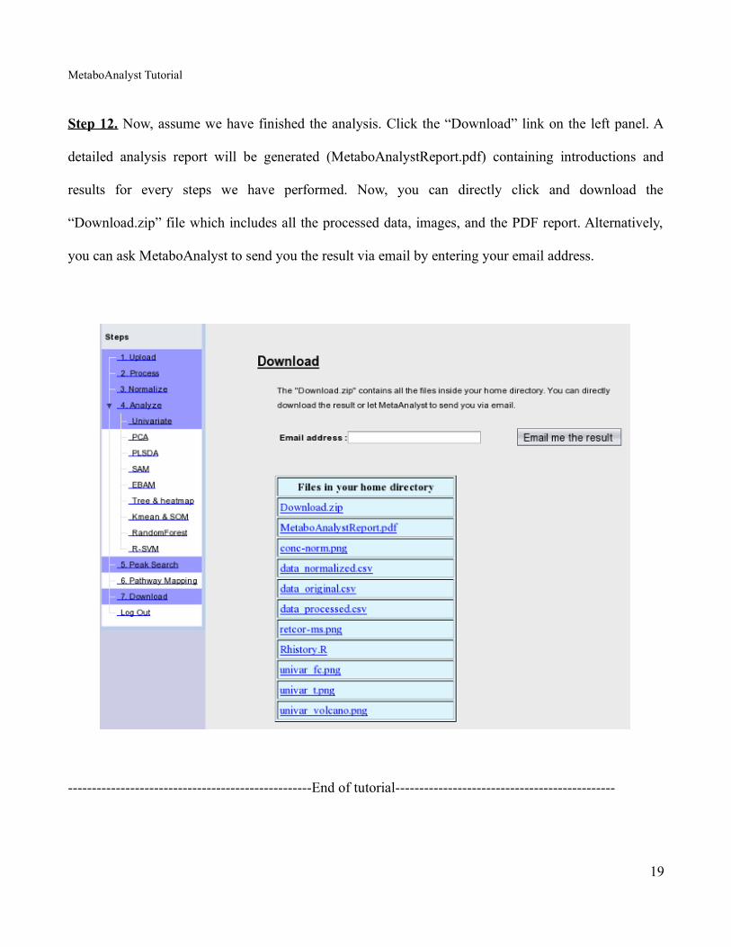
Step 12. Now, assume we have finished the analysis. Click the “Download” link on the left panel. A

detailed analysis report will be generated (MetaboAnalystReport.pdf) containing introductions and

results for every steps we have performed. Now, you can directly click and download the

“Download.zip” file which includes all the processed data, images, and the PDF report. Alternatively,

you can ask MetaboAnalyst to send you the result via email by entering your email address.

---------------------------------------------------End of tutorial----------------------------------------------

19