High-Speed Limnology: Using Advanced Sensors to InvestigateSpatial Variability in Biogeochemistry and HydrologyJohn T. Crawford,*,†,‡ Luke C. Loken,‡ Nora J. Casson,‡,§ Colin Smith,‡ Amanda G. Stone,‡

and Luke A. Winslow‡,∥

†U.S. Geological Survey, National Research Program, 3215 Marine Street, Boulder, Colorado 80303, United States‡Center for Limnology, University of WisconsinMadison, 680 North Park Street Madison, Wisconsin 53706, United States

*S Supporting Information

ABSTRACT: Advanced sensor technology is widely used inaquatic monitoring and research. Most applications focus ontemporal variability, whereas spatial variability has beenchallenging to document. We assess the capability of waterchemistry sensors embedded in a high-speed water intake systemto document spatial variability. This new sensor platformcontinuously samples surface water at a range of speeds (0 to>45 km h−1) resulting in high-density, mesoscale spatial data.These novel observations reveal previously unknown variabilityin physical, chemical, and biological factors in streams, rivers, andlakes. By combining multiple sensors into one platform, we were able to detect terrestrial−aquatic hydrologic connections in asmall dystrophic lake, to infer the role of main-channel vs backwater nutrient processing in a large river and to detect sharpchemical changes across aquatic ecosystem boundaries in a stream/lake complex. Spatial sensor data were verified in ourexamples by comparing with standard lab-based measurements of selected variables. Spatial fDOM data showed strongcorrelation with wet chemistry measurements of DOC, and optical NO3 concentrations were highly correlated with lab-basedmeasurements. High-frequency spatial data similar to our examples could be used to further understand aquatic biogeochemicalfluxes, ecological patterns, and ecosystem processes, and will both inform and benefit from fixed-site data.

■ INTRODUCTION

Advanced sensor technology has led to new and unexpectedinsights into ecosystem processes that may not have beenpossible with previous techniques.1,2 Powerful networks ofsemiautonomous sensors (e.g., FLUXNET, NEON) areincreasing our ability to measure, model, and develop theoryof biogeochemistry, hydrology, and ecosystem function.Meanwhile, lowering sensor costs and increasing the ease ofuse are enabling smaller groups and individual investigators toobserve important parameters at much-needed scales andfrequency. Pervasive examples of sensor applications in aquaticsystems include monitoring of riverine dissolved oxygen andwater discharge (by the U.S. Geological Survey and others) andmonitoring of lake chemical and physical characteristics such asdissolved oxygen, wind speed, and water temperature by theGlobal Lake Ecological Observatory Network (GLEON).Although sensor technology is becoming common in

limnological research, current applications focus almost entirelyon temporal pattern and variation. Spatial variability is rarelydocumented with sensors because of the high investment costsfor the spatial replication of such infrastructure.3 In contrast,spatial patterns have been documented for many years incoastal environments and ocean basins from large networks ofsensors (e.g., Global Drifter Program, autonomous underwatervehicles) or from cooperative research cruises. However, unlikethe open ocean, there are tens to hundreds of millions of inland

water bodies,4 and they are extremely diverse,5,6 thusprecluding easily integrated sampling techniques. Similarly,spatial patterns within small inland waterbodies are notobservable with current remote-sensing technology (althoughlarger waterbodies are more easily imaged) and may changeover short time scales (hours), thus placing them in achallenging intermediate zone in which few automatedobservation tools are appropriate. Additionally, many importantattributes of freshwaters are not detectable with current remotesensing technology, thus necessitating in situ tools.In addition to logistical challenges, conceptualizations and

long-held assumptions of aquatic ecosystems limit our ability tounderstand complex environmental phenomena. Our mentalmodels of lakes and rivers dictate “not only how data arecollected but also what data are collected and, most important,what questions are asked”.7 For example, streams and rivers aretypically studied from a fixed location, emphasizing the role ofadvection and transport of matter and energy. Less attention isgiven to longitudinal variability despite broad awareness of itsinfluence.8 Lakes, on the other hand, are typically con-ceptualized in the vertical dimension, emphasizing the roles

Received: October 8, 2014Revised: November 14, 2014Accepted: November 18, 2014

Article

pubs.acs.org/est

© XXXX American Chemical Society A dx.doi.org/10.1021/es504773x | Environ. Sci. Technol. XXXX, XXX, XXX−XXX

This is an open access article published under an ACS AuthorChoice License, which permitscopying and redistribution of the article or any adaptations for non-commercial purposes.

of stratification and vertical mixing, thus partially disregardinghorizontal patterns. But what insights can be gained fromaltering our frame of reference or expanding from singlelocations? And how might we apply powerful sensor technologyto other spatial dimensions?Past work has highlighted significant spatial variability of

water chemistry in individual aquatic ecosystems,3,9−12 butthere is a clear need to address spatial variability in additionalfreshwater ecosystems13 and in a more efficient manner. Thegoal of this paper is to present and evaluate a platform capableof rapid spatial sampling of surface waters using current sensortechnology. While we are not the first to use sensor technologyon a boat,14,15 our platform allows for easy integration ofmultiple sensors and allows for both low-speed andunprecedented high-speed sampling. In addition to describingthis new device, our goal is to present and evaluate previouslyunknown spatial patterns in an array of streams, rivers, andlakes. We also provide suggestions for future applications insupport of scientific research, engineering, management, andoutreach. Our selected examples also address practical aspectssuch as the use of spatial statistics, a consideration of aquatictransition zones, and terrestrial−aquatic connections. Each ofthese examples is geared toward the broad goal of betterunderstanding ecosystem pattern and process.

■ MATERIALS AND METHODSInstrumentation. The Fast Limnology Automated Meas-

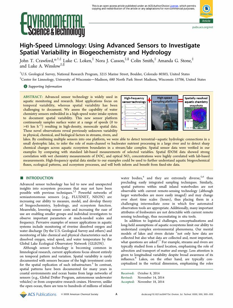
urement (FLAMe) platform is a novel flow-through systemdesigned to sample inland waters at both low (0 to ∼10 kmh−1) and high speeds (10 to >45 km h−1) (Figure 1). TheFLAMe consists of three components: an intake manifold thatattaches to the stern of a boat (having both slow- and high-speed intakes, Figure 1 and Figure S1, Supporting Informa-tion); a sensor and control box that contains hoses, valves, acirculation pump and sensor cradles (Figure S2, SupportingInformation); and a battery bank to power the electricalcomponents. The boat-mounted intake manifold serves multi-ple purposes. First, sensors are mounted inside the boat,protecting them from potential damage. Second, the intakesystem creates a constant, bubble-free water flow, thuspreventing any issues for optical sensors due to cavitation.Finally, to analyze dissolved gases, a constant water source isneeded on board. Water flow via both the slow- and high-speedintakes is regulated by the onboard impeller pump, allowing forseamless switching between slow- and high-speed operations.Any number of sensors could be integrated into the platformwith simple modifications and can be combined with commonlimnological instruments such as acoustic depth-finders. In ourexample applications we used a YSI EXO2 multiparametersonde (EXO2; Yellow Springs, OH) and a Satlantic SUNA V2optical nitrate (NO3) sensor (Halifax, NS, Canada), both

Figure 1. Photograph of the fast limnology automated measurement (FLAMe) platform water intake system attached to a moving boat; inset is acomputer rendering highlighting the two intake ports not visible in the photograph.

Environmental Science & Technology Article

dx.doi.org/10.1021/es504773x | Environ. Sci. Technol. XXXX, XXX, XXX−XXXB

integrated into the control box plumbing with flow-throughcells available from the manufacturer. Additionally, a Los GatosResearch ultraportable greenhouse gas analyzer (UGGA)(cavity enhanced absorption spectrometer; Mountain View,CA) was used to measure the dry mole fraction of carbondioxide (CO2) dissolved in surface water by equilibrating waterwith a small headspace using a sprayer-type equilibrationsystem that has previously been shown to have fast responsetimes relative to other designs16 (Figure S1, SupportingInformation). Both the EXO2 and the UGGA are capable oflogging data at 1 Hz. Because the SUNA was operated out ofthe water and on a boat during warm periods, data werecollected less frequently (∼0.1 Hz) to minimize lamp-on timeand avoid the lamp temperature cutoff of 35 °C. The EXO2sonde uses a combination of electrical and optical sensors forspecific conductivity, water temperature, pH, dissolved oxygen,turbidity, fluorescent dissolved organic matter (fDOM),chlorophyll-a fluorescenece, and phycocyanin fluorescence.The SUNA instrument measures NO3 using in situ ultravioletspectroscopy between 190 and 370 nm and has a detectionrange of 0.3−3000 μM NO3, and a precision of 2 μM NO3. TheUGGA has a reported precision of 1 ppb (by volume). In orderto translate time-series data from the instruments into spatialdata, we also logged latitude and longitude at 1 Hz with a globalpositioning system (GPS) with the Wide Area AugmentationSystem (WAAS) functionality enabled allowing for <3 maccuracy for 95% of measured coordinates. Synchronized timestamps from the EXO2, UGGA, SUNA, and GPS were used tocombine data streams into a single spatially referenced data set.The FLAMe platform was tested with a 5 m long research

boat under a wide range of velocities (idling to >45 km h−1)and wave conditions on Lake Mendota, WI. We found that thelow-draft of the intake system allowed for unencumberedoperation of the boat with no noticeable impacts on the boat’shandling or top speed. We ran a simple set of experiments todetermine the residence time of the system and the overallresponse time of the EXO2 and UGGA sensors integrated intothe platform (Supporting Information). After determining first-order response characteristics of each sensor, we tested andapplied an ordinary differential equation method to correct theraw data for significant changes in water input resulting inhigher accuracy spatial data (Supporting Information). Thegoal of this paper was not to evaluate individual sensor accuracyand precision; however, we did address sensor vs wet chemistry(dissolved fraction) measurements in two selected examples todetermine the general applicability of the platform. We havenot yet assessed the platform’s ability to properly collect andanalyze larger particles. We used the FLAMe throughout thesummer of 2014 on four distinct aquatic ecosystems, includinga small dystrophic lake, a stream/lake complex, a medium-sizedeutrophic lake, and a managed reach of the upper MississippiRiver (Table 1). Each of these applications demonstrates thespatial variability of surface water chemistry and the flexibility of

FLAMe for limnological research. Although we typically ran allinstruments at 1 Hz, we present parameters selectively forbrevity.

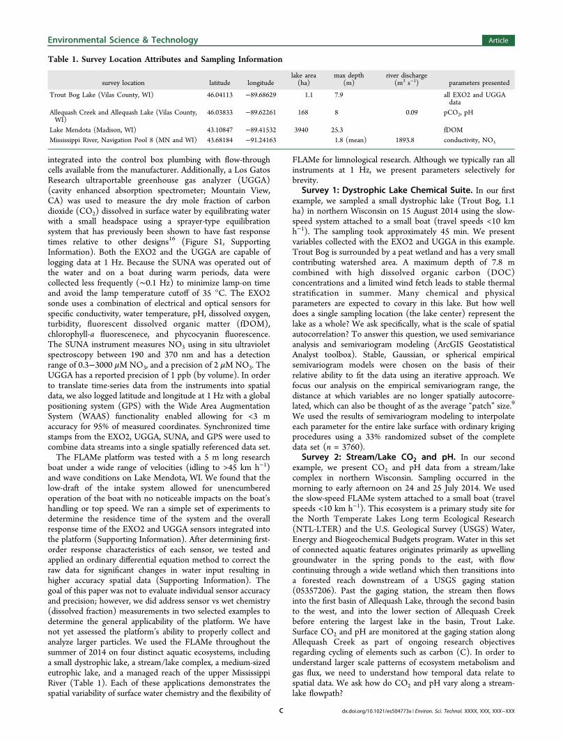
Survey 1: Dystrophic Lake Chemical Suite. In our firstexample, we sampled a small dystrophic lake (Trout Bog, 1.1ha) in northern Wisconsin on 15 August 2014 using the slow-speed system attached to a small boat (travel speeds <10 kmh−1). The sampling took approximately 45 min. We presentvariables collected with the EXO2 and UGGA in this example.Trout Bog is surrounded by a peat wetland and has a very smallcontributing watershed area. A maximum depth of 7.8 mcombined with high dissolved organic carbon (DOC)concentrations and a limited wind fetch leads to stable thermalstratification in summer. Many chemical and physicalparameters are expected to covary in this lake. But how welldoes a single sampling location (the lake center) represent thelake as a whole? We ask specifically, what is the scale of spatialautocorrelation? To answer this question, we used semivarianceanalysis and semivariogram modeling (ArcGIS GeostatisticalAnalyst toolbox). Stable, Gaussian, or spherical empiricalsemivariogram models were chosen on the basis of theirrelative ability to fit the data using an iterative approach. Wefocus our analysis on the empirical semivariogram range, thedistance at which variables are no longer spatially autocorre-lated, which can also be thought of as the average “patch” size.9

We used the results of semivariogram modeling to interpolateeach parameter for the entire lake surface with ordinary krigingprocedures using a 33% randomized subset of the completedata set (n = 3760).

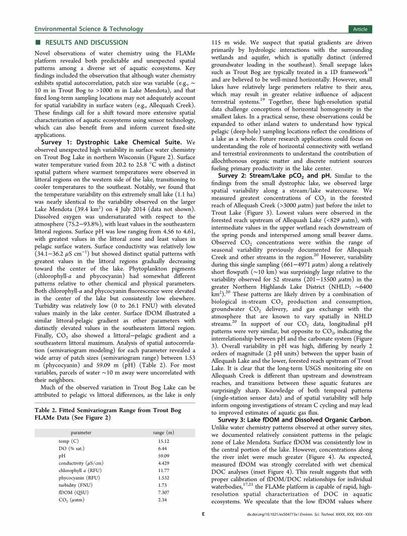
Survey 2: Stream/Lake CO2 and pH. In our secondexample, we present CO2 and pH data from a stream/lakecomplex in northern Wisconsin. Sampling occurred in themorning to early afternoon on 24 and 25 July 2014. We usedthe slow-speed FLAMe system attached to a small boat (travelspeeds <10 km h−1). This ecosystem is a primary study site forthe North Temperate Lakes Long term Ecological Research(NTL-LTER) and the U.S. Geological Survey (USGS) Water,Energy and Biogeochemical Budgets program. Water in this setof connected aquatic features originates primarily as upwellinggroundwater in the spring ponds to the east, with flowcontinuing through a wide wetland which then transitions intoa forested reach downstream of a USGS gaging station(05357206). Past the gaging station, the stream then flowsinto the first basin of Allequash Lake, through the second basinto the west, and into the lower section of Allequash Creekbefore entering the largest lake in the basin, Trout Lake.Surface CO2 and pH are monitored at the gaging station alongAllequash Creek as part of ongoing research objectivesregarding cycling of elements such as carbon (C). In order tounderstand larger scale patterns of ecosystem metabolism andgas flux, we need to understand how temporal data relate tospatial data. We ask how do CO2 and pH vary along a stream-lake flowpath?

Table 1. Survey Location Attributes and Sampling Information

survey location latitude longitudelake area(ha)

max depth(m)

river discharge(m3 s−1) parameters presented

Trout Bog Lake (Vilas County, WI) 46.04113 −89.68629 1.1 7.9 all EXO2 and UGGAdata

Allequash Creek and Allequash Lake (Vilas County,WI)

46.03833 −89.62261 168 8 0.09 pCO2, pH

Lake Mendota (Madison, WI) 43.10847 −89.41532 3940 25.3 fDOMMississippi River, Navigation Pool 8 (MN and WI) 43.68184 −91.24163 1.8 (mean) 1893.8 conductivity, NO3

Environmental Science & Technology Article

dx.doi.org/10.1021/es504773x | Environ. Sci. Technol. XXXX, XXX, XXX−XXXC

Survey 3: Lake fDOM and Dissolved Organic Carbon.In our third example, we present fDOM data collected between08:00 and 12:00 on 4 July 2014 on Lake Mendota (Madison,WI), a medium-sized eutrophic lake. We sampled the majorityof the lake at high speed (>40 km h−1) in order to capture a fullspatial “snapshot”. In addition to the sensor data, we collecteddiscrete water samples for DOC concentration. We predictedthat fDOM and DOC would be positively correlated in thisecosystem.17 Water chemistry samples were collected intoplastic bottles while the boat was stopped and free-floatingusing the slow-speed intake and were then capped and storedon ice. Each sample was filtered (0.45 μm) in the lab within 3 hof collection. Filtered DOC samples were analyzed according toprotocols established by the NTL-LTER (https://lter.limnology.wisc.edu) using a Shimadzu TOC-V-csh total organiccarbon analyzer. Using this data set, we ask how homogeneousis the surface mixed layer with respect to DOC concentrations?We again use semivariogram modeling and focus on the rangeparameter.Survey 4: River Conductivity and NO3. In our final

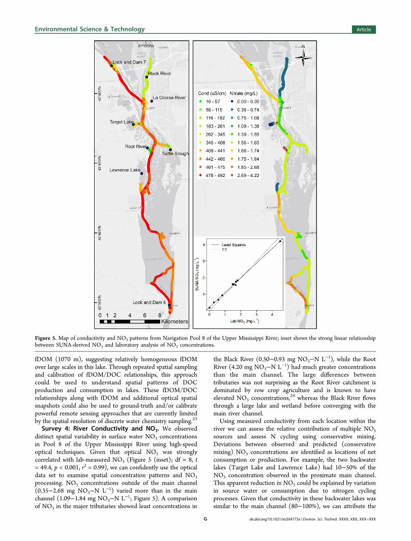
example, we present conductivity and NO3 data collected onNavigation Pool 8 of the Upper Mississippi River (near LaCrosse, WI) on 21−22 July 2014. We primarily used the high-speed system (>30 km h−1) to capture spatial variability. Due tothe large size of the reach, we combined data collected over thecourse of 2 days, primarily in the morning and early afternoon

periods. River discharge (measured at Dam 8) during oursampling was 1893.8 and 1775.4 m3 s−1 on the 21st and 22nd,respectively. Our sampling path included sections above andbelow Lock and Dam 7, the main navigation channel, threetributaries (Black River, La Crosse River, and Root River), twobackwater lakes (Target Lake and Lawrence Lake), a backwaterchannel (Turtle Slough), and immediately upstream from Lockand Dam 8. In this example, we ask how does NO3 vary amongthe major inputs to Pool 8? Additionally, we investigated howNO3 compared between the various backwater river sectionsand the main channel. Using conductivity as a conservativetracer, we identified locations with potentially elevated NO3

cycling.To confirm SUNA measurements, we collected discrete

water samples at 10 locations spanning the range of SUNANO3. River water was filtered (0.45 μm) into new 20 mL plasticscintillation vials. Samples were stored on ice and frozen within6 h of collection. Lab NO3 samples were analyzed according toprotocols established by the North Temperate Lakes LTERusing an Astoria-Pacific Astoria 2 segmented flow autoanalyzerand reported as mg NO3−N L−1. We assessed the relationshipbetween the traditional lab method and the SUNA sensor usinglinear regression.

Figure 2. Results of FLAMe survey of a small dystrophic lake (Trout Bog) showing all measured variables from the EXO2 and UGGA instruments;values were interpolated at the 0.25 m scale using semivariogram analysis (Table 2) and ordinary kriging; top-left panel includes the sampling pathand background aerial imagery.

Environmental Science & Technology Article

dx.doi.org/10.1021/es504773x | Environ. Sci. Technol. XXXX, XXX, XXX−XXXD

■ RESULTS AND DISCUSSION

Novel observations of water chemistry using the FLAMeplatform revealed both predictable and unexpected spatialpatterns among a diverse set of aquatic ecosystems. Keyfindings included the observation that although water chemistryexhibits spatial autocorrelation, patch size was variable (e.g., ∼10 m in Trout Bog to >1000 m in Lake Mendota), and thatfixed long-term sampling locations may not adequately accountfor spatial variability in surface waters (e.g., Allequash Creek).These findings call for a shift toward more extensive spatialcharacterization of aquatic ecosystems using sensor technology,which can also benefit from and inform current fixed-siteapplications.Survey 1: Dystrophic Lake Chemical Suite. We

observed unexpected high variability in surface water chemistryon Trout Bog Lake in northern Wisconsin (Figure 2). Surfacewater temperature varied from 20.2 to 25.8 °C with a distinctspatial pattern where warmest temperatures were observed inlittoral regions on the western side of the lake, transitioning tocooler temperatures to the southeast. Notably, we found thatthe temperature variability on this extremely small lake (1.1 ha)was nearly identical to the variability observed on the largerLake Mendota (39.4 km2) on 4 July 2014 (data not shown).Dissolved oxygen was undersaturated with respect to theatmosphere (75.2−93.8%), with least values in the southeasternlittoral regions. Surface pH was low ranging from 4.56 to 4.61,with greatest values in the littoral zone and least values inpelagic surface waters. Surface conductivity was relatively low(34.1−36.2 μS cm−1) but showed distinct spatial patterns withgreatest values in the littoral regions gradually decreasingtoward the center of the lake. Phytoplankton pigments(chlorophyll-a and phycocyanin) had somewhat differentpatterns relative to other chemical and physical parameters.Both chlorophyll-a and phycocyanin fluorescence were elevatedin the center of the lake but consistently low elsewhere.Turbidity was relatively low (0 to 26.1 FNU) with elevatedvalues mainly in the lake center. Surface fDOM illustrated asimilar littoral-pelagic gradient as other parameters withdistinctly elevated values in the southeastern littoral region.Finally, CO2 also showed a littoral−pelagic gradient and asoutheastern littoral maximum. Analysis of spatial autocorrela-tion (semivariogram modeling) for each parameter revealed awide array of patch sizes (semivariogram range) between 1.53m (phycocyanin) and 59.09 m (pH) (Table 2). For mostvariables, parcels of water ∼10 m away were uncorrelated withtheir neighbors.Much of the observed variation in Trout Bog Lake can be

attributed to pelagic vs littoral differences, as the lake is only

115 m wide. We suspect that spatial gradients are drivenprimarily by hydrologic interactions with the surroundingwetlands and aquifer, which is spatially distinct (inferredgroundwater loading in the southeast). Small seepage lakessuch as Trout Bog are typically treated in a 1D framework18

and are believed to be well-mixed horizontally. However, smalllakes have relatively large perimeters relative to their area,which may result in greater relative influence of adjacentterrestrial systems.19 Together, these high-resolution spatialdata challenge conceptions of horizontal homogeneity in thesmallest lakes. In a practical sense, these observations could beexpanded to other inland waters to understand how typicalpelagic (deep-hole) sampling locations reflect the conditions ofa lake as a whole. Future research applications could focus onunderstanding the role of horizontal connectivity with wetlandand terrestrial environments to understand the contribution ofallochthonous organic matter and discrete nutrient sourcesfueling primary productivity in the lake center.

Survey 2: Stream/Lake pCO2 and pH. Similar to thefindings from the small dystrophic lake, we observed largespatial variability along a stream/lake watercourse. Wemeasured greatest concentrations of CO2 in the forestedreach of Allequash Creek (>3000 μatm) just before the inlet toTrout Lake (Figure 3). Lowest values were observed in theforested reach upstream of Allequash Lake (<829 μatm), withintermediate values in the upper wetland reach downstream ofthe spring ponds and interspersed among small beaver dams.Observed CO2 concentrations were within the range ofseasonal variability previously documented for AllequashCreek and other streams in the region.20 However, variabilityduring this single sampling (661−4971 μatm) along a relativelyshort flowpath (∼10 km) was surprisingly large relative to thevariability observed for 52 streams (201−15500 μatm) in thegreater Northern Highlands Lake District (NHLD; ∼6400km2).20 These patterns are likely driven by a combination ofbiological in-stream CO2 production and consumption,groundwater CO2 delivery, and gas exchange with theatmosphere that are known to vary spatially in NHLDstreams.20 In support of our CO2 data, longitudinal pHpatterns were very similar, but opposite to CO2, indicating theinterrelationship between pH and the carbonate system (Figure3). Overall variability in pH was high, differing by nearly 2orders of magnitude (2 pH units) between the upper basin ofAllequash Lake and the lower, forested reach upstream of TroutLake. It is clear that the long-term USGS monitoring site onAllequash Creek is different than upstream and downstreamreaches, and transitions between these aquatic features aresurprisingly sharp. Knowledge of both temporal patterns(single-station sensor data) and of spatial variability will helpinform ongoing investigations of stream C cycling and may leadto improved estimates of aquatic gas flux.

Survey 3: Lake fDOM and Dissolved Organic Carbon.Unlike water chemistry patterns observed at other survey sites,we documented relatively consistent patterns in the pelagiczone of Lake Mendota. Surface fDOM was consistently low inthe central portion of the lake. However, concentrations alongthe river inlet were much greater (Figure 4). As expected,measured fDOM was strongly correlated with wet chemicalDOC analyses (inset Figure 4). This result suggests that withproper calibration of fDOM/DOC relationships for individualwaterbodies,17,21 the FLAMe platform is capable of rapid, high-resolution spatial characterization of DOC in aquaticecosystems. We speculate that the low fDOM values where

Table 2. Fitted Semivariogram Range from Trout BogFLAMe Data (See Figure 2)

parameter range (m)

temp (C) 15.12DO (% sat.) 6.44pH 59.09conductivity (μS/cm) 4.429chlorophyll a (RFU) 11.77phycocyanin (RFU) 1.532turbidity (FNU) 1.73fDOM (QSU) 7.307CO2 (μatm) 2.34

Environmental Science & Technology Article

dx.doi.org/10.1021/es504773x | Environ. Sci. Technol. XXXX, XXX, XXX−XXXE

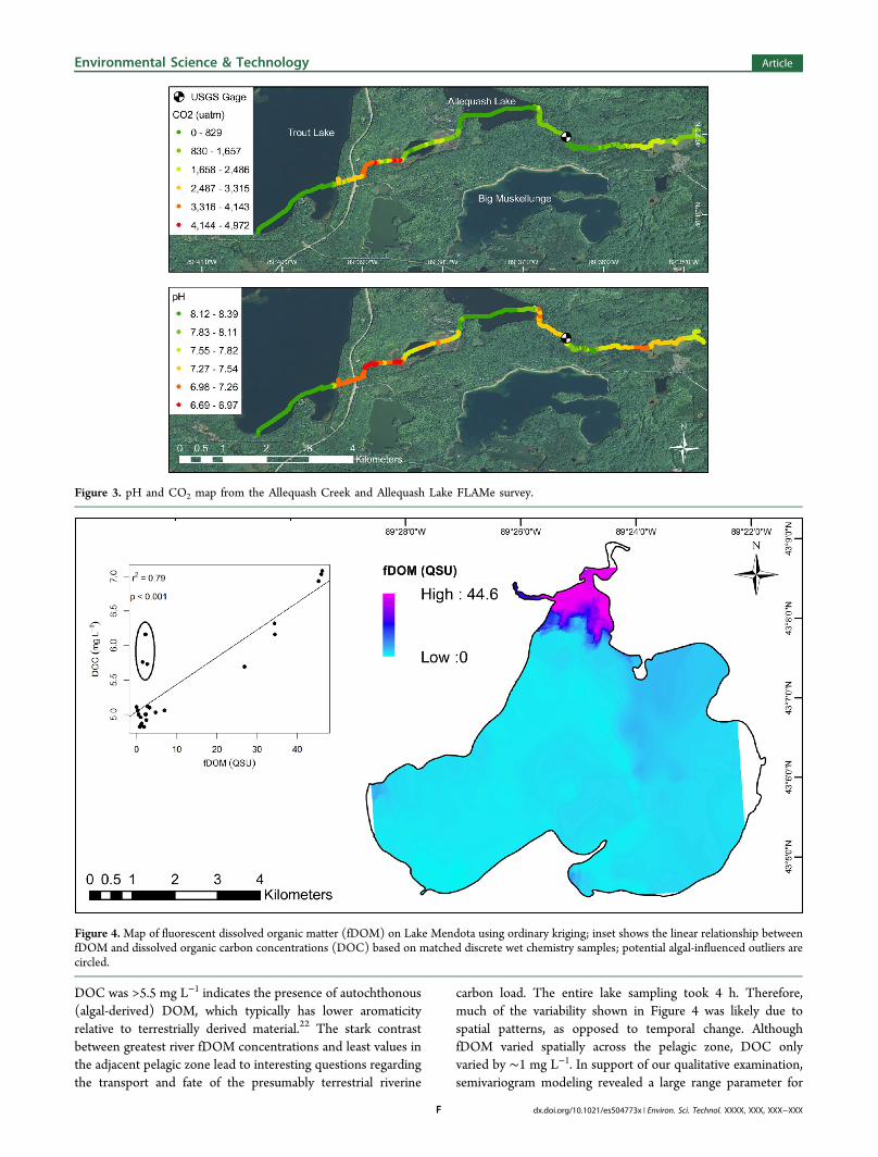
DOC was >5.5 mg L−1 indicates the presence of autochthonous(algal-derived) DOM, which typically has lower aromaticityrelative to terrestrially derived material.22 The stark contrastbetween greatest river fDOM concentrations and least values inthe adjacent pelagic zone lead to interesting questions regardingthe transport and fate of the presumably terrestrial riverine

carbon load. The entire lake sampling took 4 h. Therefore,much of the variability shown in Figure 4 was likely due tospatial patterns, as opposed to temporal change. AlthoughfDOM varied spatially across the pelagic zone, DOC onlyvaried by ∼1 mg L−1. In support of our qualitative examination,semivariogram modeling revealed a large range parameter for

Figure 3. pH and CO2 map from the Allequash Creek and Allequash Lake FLAMe survey.

Figure 4.Map of fluorescent dissolved organic matter (fDOM) on Lake Mendota using ordinary kriging; inset shows the linear relationship betweenfDOM and dissolved organic carbon concentrations (DOC) based on matched discrete wet chemistry samples; potential algal-influenced outliers arecircled.

Environmental Science & Technology Article

dx.doi.org/10.1021/es504773x | Environ. Sci. Technol. XXXX, XXX, XXX−XXXF

fDOM (1070 m), suggesting relatively homogeneous fDOMover large scales in this lake. Through repeated spatial samplingand calibration of fDOM/DOC relationships, this approachcould be used to understand spatial patterns of DOCproduction and consumption in lakes. These fDOM/DOCrelationships along with fDOM and additional optical spatialsnapshots could also be used to ground-truth and/or calibratepowerful remote sensing approaches that are currently limitedby the spatial resolution of discrete water chemistry sampling.23

Survey 4: River Conductivity and NO3. We observeddistinct spatial variability in surface water NO3 concentrationsin Pool 8 of the Upper Mississippi River using high-speedoptical techniques. Given that optical NO3 was stronglycorrelated with lab-measured NO3 (Figure 5 (inset); df = 8, t= 49.4, p < 0.001, r2 = 0.99), we can confidently use the opticaldata set to examine spatial concentration patterns and NO3

processing. NO3 concentrations outside of the main channel(0.35−2.68 mg NO3−N L−1) varied more than in the mainchannel (1.09−1.84 mg NO3−N L−1; Figure 5). A comparisonof NO3 in the major tributaries showed least concentrations in

the Black River (0.50−0.93 mg NO3−N L−1), while the RootRiver (4.20 mg NO3−N L−1) had much greater concentrationsthan the main channel. The large differences betweentributaries was not surprising as the Root River catchment isdominated by row crop agriculture and is known to haveelevated NO3 concentrations,

24 whereas the Black River flowsthrough a large lake and wetland before converging with themain river channel.Using measured conductivity from each location within the

river we can assess the relative contribution of multiple NO3

sources and assess N cycling using conservative mixing.Deviations between observed and predicted (conservativemixing) NO3 concentrations are identified as locations of netconsumption or production. For example, the two backwaterlakes (Target Lake and Lawrence Lake) had 10−50% of theNO3 concentration observed in the proximate main channel.This apparent reduction in NO3 could be explained by variationin source water or consumption due to nitrogen cyclingprocesses. Given that conductivity in these backwater lakes wassimilar to the main channel (80−100%), we can attribute the

Figure 5. Map of conductivity and NO3 patterns from Navigation Pool 8 of the Upper Mississippi River; inset shows the strong linear relationshipbetween SUNA-derived NO3 and laboratory analysis of NO3 concentrations.

Environmental Science & Technology Article

dx.doi.org/10.1021/es504773x | Environ. Sci. Technol. XXXX, XXX, XXX−XXXG

reduction of NO3 to uptake and removal processes. Backwaterregions of Pool 8 have previously been identified as havingelevated denitrification capacity due to greater amounts ofsediment organic matter and greater biological uptake resultingfrom N limitation in late summer.25,26 In contrast, mainchannel NO3 concentrations were more homogeneous,indicating the greater role of advection relative to uptake.27

Further identification of spatially explicit NO3 sources and sinks(as well as process rates) in the Upper Mississippi River maylead to a better understanding of the fate of anthropogenicNO3. Somewhat surprisingly, NO3 variability in Pool 8 during asingle summer day (0.35−2.68 mg NO3−N L−1) was nearlyequivalent to the two-year range (0.22 to 2.97 mg NO3−N L−1)observed in the Lower Mississippi River with a similar sensorlocated at a fixed-station.28 Future work could simultaneouslyassess the scales of spatial and temporal variability as they relateto biogeochemical processes and ecosystem function.Assessment and Future Applications. We have

presented several examples of pervasive spatial variability inaquatic ecosystems using a novel sampling platform. Theseexamples of spatial water chemistry highlight some possibilitiesof basic biogeochemical mapping that may be useful on theirown as a management tool. However, cartographic representa-tions of these data sets are simply the first step in dataexploration, similar to making a histogram or scatterplot oftypical data. There is a clear need to translate spatialrepresentations of water chemistry into a process-basedunderstanding, and to address fundamental questions regardingspatial variation.Spatial sampling approaches like the one demonstrated here

can supplement and benefit from fixed-station time-series data(streams and rivers), depth profiles (lakes), and other standardaquatic data sets. Integration of these multiple approaches willlikely yield new insights and breakthroughs in the study offreshwater ecosystems, but their assimilation will likely beecosystem and question-specific. The goal should not be toeliminate fixed sensor installations or long-term samplingschemes, but rather to supplement those with spatial snapshotsat the surface. Potential combinations include: sampling laketemperature and dissolved oxygen during lake mixis usingdepth-profiling buoys and spatial surveys to understand mixingprocesses; tracking nutrient exchange between river channelsand backwaters in relation to changes in the hydrograph; andtracing distinct water plumes in transit past observing stations.Despite the ability to sample aquatic ecosystems at high

speeds using the FLAMe platform, care must be taken wheninterpreting these results for larger ecosystems. Sampling eventslasting longer than a few hours will inevitably be impacted bytemporal variability in addition to spatial variability. Forinstance, diel oxygen excursions driven by primary productionwould impact the observed dissolved oxygen variability in spaceif sampled over longer time periods (e.g., > 4 h). Ourassessments of spatial variability are also limited by the accuracyand precision of the sensors used. While we have provided anexample of how to evaluate response times and correct thesehigh-frequency data (Supporting Information), evaluatingsensor performance in other applications is essential.Further insights might be gained by altering reference frames

in support of scientific research, engineering, management, andoutreach. We suggest that the FLAMe platform could be usedto rapidly assess spatial variability before and after major events(e.g., storms, stratification) and to inform future and ongoingecosystem studies. Gridded data (e.g., Figure 2) could be used

to ground-truth remote sensing products23,29 and ecosystemmodels. Investigators could use the platform for efficientreconnaissance of discrete chemical influences such as urbandischarges and other point sources.30 Development ofinnovative calibrations and transfer functions could lead tomaps of socially valuable ecosystem metrics that could appeal tothe broader public. Further, time-series of spatially explicit datacould be leveraged to generate water forecasts (perhaps focusedon littoral areas) where there are potential health concernsfrom harmful algal blooms and other water quality issues.

■ ASSOCIATED CONTENT*S Supporting InformationDescriptions of equipment and experiments. This material isavailable free of charge via the Internet at http://pubs.acs.org/

■ AUTHOR INFORMATIONCorresponding Author*E-mail: jtcrawford@wisc.edu.Present Addresses§University of Winnipeg, Department of Geography, 515Portage Ave, Winnipeg, Manitoba, Canada.∥U.S. Geological Survey, Center for Integrated Data Analytics,Middleton, WI, 53562.NotesThe authors declare no competing financial interest.

■ ACKNOWLEDGMENTSWe thank Emily Stanley for helpful discussions and commentson earlier drafts of the manuscript. We thank Dave Harring fortechnical support during the construction of the water intakesystem. We are grateful to the three anonymous reviewers whoprovided helpful feedback on the manuscript. Partial fundingwas provided by the U.S. Geological Survey Water, Energy, andBiogeochemical Budgets Program, the U.S Geological SurveyLand Carbon Project, and the North Temperate Lakes LTERprogram. Any use of trade or product names is for descriptivepurposes only and does not imply endorsement by the U.S.Government. This material is based upon work supported bythe National Science Foundation under Cooperative Agree-ment DEB-0822700, NTL LTER.

■ REFERENCES(1) Kirchner, J. W.; Feng, X.; Neal, C.; Robson, A. J. The finestructure of water-quality dynamics: the (high-frequency) wave of thefuture. Hydrological Processes 2004, 18, 1353−1359.(2) Porter, J.; Arzberger, P.; Braun, H.; Bryant, P.; Gage, S.; Hansen,T.; Hanson, P.; Lin, C.; Lin, F.; Kratz, T.; Michener, W.; Shapiro, S.;Williams, T. Wireless sensor networks for ecology. BioScience 2005, 55,561−572.(3) Van de Bogert, M. C.; Bade, D. L.; Carpenter, S. R.; Cole, J. J.;Pace, M. L.; Hanson, P. C.; Langman, O. C. Spatial heterogeneitystrongly affects estimates of ecosystem metabolism in two northtemperate lakes. Limnol. Oceanogr. 2012, 57, 1689−1700.(4) McDonald, C. P.; Rover, J. A.; Stets, E. G.; Striegl, R. G. Theregional abundance and size distribution of lakes and reservoirs in theUnited States and implications for estimates of global lake extent.Limnol. Oceanogr. 2012, 57, 597−606.(5) Downing, J. A.; Cole, J. J.; Duarte, C. M.; Middleburg, J. J.;Melack, J. M.; Prairie, Y. T.; Kortelainen, P.; Striegl, R. G.; McDowell,W. H.; Tranvik, L. J. Global abundance and size distribution of streamsand rivers. Inland Waters 2012, 2, 229−236.(6) Cole, J. J.; Prairie, Y. T.; Caraco, N. F.; McDowell, W. H.;Tranvik, L. J.; Striegl, R. G.; Duarte, C. M.; Kortelainen, P.; Downing,

Environmental Science & Technology Article

dx.doi.org/10.1021/es504773x | Environ. Sci. Technol. XXXX, XXX, XXX−XXXH

J. A.; Middleburg, J. J.; Melack, J. Plumbing the global carbon cycle:Integrating inland waters into the terrestrial carbon budget. Ecosystems2007, 10, 171−184.(7) Doyle, M. W.; Ensign, S. H. Alternative reference frames in riversystem science. BioScience 2009, 59, 499−510.(8) Vannote, R. L.; Minshall, G. W.; Cummins, K. W.; Sedell, J. R.;Cushing, C. E. The river continuum concept. Can. J. Fish. Aquat. Sci.1980, 37, 130−137.(9) Dent, C. L.; Grimm, N. B. Spatial heterogeneity of stream waternutrient concentrations over successional time. Ecology 1999, 80,2283−2298.(10) Vadeboncoeur, Y.; Kalff, J.; Christoffersen, K.; Jeppesen, E.Substratum as a driver of variation in periphyton chlorophyll andproductivity in lakes. J. North Am. Bentholog. Soc. 2006, 25, 379−392.(11) Hoffman, H. Spatiotemporal distribution patterns of dissolvedmethane in lakes: How accurate are the current estimations of thediffusive flux path? Geophys. Res. Lett. 2013, 40, 2779−2784.(12) Schilder, J.; Bastviken, D.; van Hardenbroek, M.; Kankaala, P.;Rinta, P.; Stotter, T.; Heiri, O. Spatial heterogeneity and lakemorphology affect diffusive greenhouse gas emission estimates oflakes. Geophys. Res. Lett. 2013, 40, 5752−5756.(13) Palmer, M. A.; Hakenkamp, C. C.; Nelson-Baker, K. Ecologicalheterogeneity in streams: why variance matters. J. North Am. Bentholog.Soc. 1997, 16, 189−202.(14) Hondzo, M.; Voller, V. R.; Morris, M.; Foufoula-Georgiou, E.;Finlay, J.; Ganti, V.; Power, M. E. Estimating and scaling streamecosystem metabolism along channels with heterogeneous substrate.Ecohydrology 2013, 6, 679−688.(15) Maher, D. T.; Santos, I. R.; Leuven, J.R.F.W; Oakes, J. M.; Erler,D. V.; Carvalho, M. C.; Eyre, B. D. Novel use of cavity ring-downspectroscopy to investigate aquatic carbon cycling from microbial toecosystem scales. Environ. Sci. Technol. 2013, 47, 12938−12945.(16) Santos, I. R.; Maher, D. T.; Eyre, B. D. Coupling automatedradon and carbon dioxide measurements in coastal waters. Environ. Sci.Technol. 2012, 46, 7685−7691.(17) Spencer, R. G. M.; Aiken, G. R.; Dornblaser, M. M.; Butler, K.D.; Holmes, R. M.; Fiske, G.; Mann, P. J.; Stubbins, A. Chromophoricdissolved organic matter export from U.S. Rivers. Geophys. Res. Lett.2013, 40, 1575−1579.(18) Read, J. S.; Rose, K. C. Physical responses of small temperatelakes to variation in dissolved organic carbon concentrations. Limnol.Oceanogr. 2013, 58, 921−931.(19) Winslow, L. A.; Read, J. S.; Hanson, P. C.; Stanley, E. H. Lakeshoreline in the contiguous United States: quantity, distribution andsensitivity to observation resolution. Freshwater Biol. 2014, 59, 213−223.(20) Crawford, J. T.; Lottig, N. R.; Stanley, E. H.; Walker, J. F.;Hanson, P. C.; Finlay, J. C.; Striegl, R. G. CO2 and CH4 emissionsfrom streams in a lake-rich landscape: Patterns, controls, and regionalsignificance. Global Biogeochem. Cycles 2014, 28, 197−210.(21) Downing, B. D.; Pellerin, B. A.; Bergamaschi, B. A.; Saraceno, J.;Kraus, T. E. C. Seeing the light: The effects of particles, temperatureand inner filtering on in situ CDOM fluorescence in rivers andstreams. Limnol. Oceanogr.: Methods 2012, 10, 767−775.(22) Weishaar, J. L.; Aiken, G. R.; Bergamaschi, B. A.; Fram, M. S.;Fujii, R.; Mopper, K. Evaluation of specific ultraviolet absorbance as anindicator of the chemical composition and reactivity of dissolvedorganic carbon. Environ. Sci. Technol. 2003, 37, 4702−4708.(23) Brezonik P. L., Olmanson L. G., Finlay J. C., Bauer M. E. Factorsaffecting the measurement of CDOM by remote sensing of opticallycomplex inland waters. Remote Sensing of Environment, 2014 http://dx.doi.org/10.1016/j.rse.2014.04.033.(24) Minnesota Pollution Control Agency Root River watershedmonitoring and assessment report, 2012, wq-ws3-070400086.(25) Strauss, E. A.; Richardson, W. B.; Cavanaugh, J. C.; Bartsch, L.A.; Kreiling, R. M.; Standorf, A. J. Variability and regulation ofdenitrification in an Upper Mississippi River backwater. J. North Am.Bentholog. Soc. 2006, 25, 596−606.

(26) Giblin, S. M.; Houser, J. N.; Sullivan, J. F.; Langrehr, H. A.;Rogala, J. T.; Campbell, B. D. Thresholds in the response of free-floating plant abundance to variation in hydraulic connectivity,nutrients, and macrophyte abundance in a large floodplain river.Wetlands 2014, 34, 413−425.(27) Alexander, R. B.; Smith, R. A.; Schwarz, G. E. Effect of streamchannel size on the delivery of nitrogen to the Gulf of Mexico. Nature2000, 403.(28) Pellerin, B. A.; Bergamaschi, B. A.; Gilliom, R. J.; Crawford, C.G.; Saraceno, J.; Frederick, C. P.; Downing, B. D.; Murphy, J. C.Mississippi River nitrate loads form high frequency sensor measure-ments and regression-based load estimation. Environ. Sci. Technol.2014, 48, 12612−12619.(29) Matthews, M. W.; Bernard, S.; Winter, K. Remote sensing ofcyanobacteria-dominant algal blooms and water quality parameters inZeekoevlei, a small hypereutrophic lake, using MERIS. Remote SensingEnviron. 2010, 114, 2070−2087.(30) Bonvin, F.; Rutler, R.; Chevre, N.; Halder, J.; Kohn, T. Spatialand temporal presence of a wastewater-derived micropollutant plumein Lake Geneva. Environ. Sci. Technol. 2011, 45, 4702−4709.

Environmental Science & Technology Article

dx.doi.org/10.1021/es504773x | Environ. Sci. Technol. XXXX, XXX, XXX−XXXI