1

High SNR Analysis for MIMO Broadcast

Channels: Dirty Paper Coding vs. Linear

PrecodingJuyul Lee and Nihar Jindal

Department of Electrical and Computer Engineering

University of Minnesota

Minneapolis, MN 55455, USA

E-mail: {juyul,nihar}@umn.edu

Abstract

We study the MIMO broadcast channel and compare the achievable throughput for the optimal

strategy of dirty paper coding to that achieved with sub-optimal and lower complexity linear precoding

(e.g., zero-forcing and block diagonalization) transmission. Both strategies utilize all available spatial

dimensions and therefore have the same multiplexing gain, but an absolute difference in terms of

throughput does exist. The sum rate difference between the two strategies is analytically computed at

asymptotically high SNR, and it is seen that this asymptotic statistic provides an accurate characterization

at even moderate SNR levels. Furthermore, the difference is not affected by asymmetric channel behavior

when each user a has different average SNR. Weighted sum rate maximization is also considered, and a

similar quantification of the throughput difference between the two strategies is performed. In the process,

it is shown that allocating user powers in direct proportion to user weights asymptotically maximizes

weighted sum rate. For multiple antenna users, uniform power allocation across the receive antennas is

applied after distributing power proportional to the user weight.

Index Terms

Multiple antenna or MIMO, broadcast channel, high SNR analysis, zero-forcing, block diagonaliza-

tion, weighted sum rate.

2

I. INTRODUCTION

The multiple antenna broadcast channel (BC) has recently been the subject of tremendous interest,

primarily due to the realization that such a channel can provide MIMO spatial multiplexing benefits

without requiring multiple antenna elements at the mobile devices [1]. Indeed, it is now well known

that dirty paper coding (DPC) achieves the capacity region of the multiple antenna BC [2]. However,

implementation of DPC requires significant additional complexity at both transmitter and receiver, and

the problem of finding practical dirty paper codes that approach the capacity limit is still unsolved.

On the other hand, linear precoding is a low complexity but sub-optimal transmission technique (with

complexity roughly equivalent to point-to-point MIMO) that is able to transmit the same number of data

streams as a DPC-based system. Linear precoding therefore achieves the same multiplexing gain (which

characterizes the slope of the capacity vs. SNR) curve) as DPC, but incurs an absolute rate/power offset

relative to DPC. The contribution of this work is the quantification of this rate/power offset.

In this work, we apply the high SNR affine approximation [3] to the sum rate capacity (DPC) and

to the linear precoding sum rate. Both approximations have the same slope (i.e., multiplexing gain), but

by characterizing the difference in the additive terms the rate/power offset between the two strategies is

determined. By averaging the per-channel realization rate offset over the iid Rayleigh fading distribution

we are able to derive very simple expressions for the average rate offset as a function of only the number

of transmit and receive antennas and users for systems in which the aggregate number of receive antennas

is no larger than the number of transmit antennas.

Note that previous work has analyzed the ratio between the sum rate capacity and the linear precoding

sum rate [4][5]. In this work we alternatively study the absolute difference between these quantities, which

appears to be a more meaningful metric precisely because both strategies provide the same multiplexing

gain.

In addition to sum rate, we also study weighted sum rate maximization (using DPC and linear

precoding) and provide simple expressions for the rate offsets in this scenario. One of the most interesting

results is that weighted sum rate (for either DPC or linear precoding) is maximized at asymptotically high

SNR by allocating power directly proportional to user weights. A similar result was recently observed

in [6] in the context of parallel single-user channels (e.g., for OFDMA systems). Because the linear

precoding strategies we study result in parallel channels, the result of [6] shows that it is asymptotically

optimal to allocate power in direct proportion to user weights whenever linear precoding is used. By

showing that weighted sum rate maximization when DPC is employed can also be simplified to power

3

allocation over parallel channels, we are able to show that the same strategy is also asymptotically optimal

for DPC. To illustrate the utility of this simple yet asymptotically optimal power allocation policy, we

apply it to a system employing queue-based scheduling (at finite SNR’s) and see that it performs extremely

close to the true optimal weighted sum rate maximization.

This paper is organized as follows: Section II presents the system model and Section III introduces the

high SNR capacity approximation from [3]. Section IV describes dirty paper coding and linear precoding

and derives simple expressions for their sum rates at high SNR, and in Section V the relative rate/power

offsets between DPC and linear precoding are computed. Section VI extends the analysis to weighted

sum rate maximization and considers a queue-based system with the weighted sum rate solution. We

conclude in Section VII.

II. SYSTEM MODEL

We consider a K-user Gaussian MIMO BC in which the transmitter has M antennas and each receiver

has N antennas with M ≥ KN , i.e., the number of transmit antennas is no smaller than the aggregate

number of receive antennas. The received signal yk of user k is given by

yk = Hkx + nk, k = 1, · · · ,K, (1)

where Hk(∈ CN×M ) is the channel gain matrix for user k, x is the transmit signal vector having a

power constraint tr(E[xxH ]) ≤ P , and nk (k = 1, · · · ,K) is complex Gaussian noise with unit variance

per vector component (i.e., E[nHk nk] = I). We assume that the transmitter has perfect knowledge of all

channel matrices and each receiver has perfect knowledge of its own channel matrix. For the sake of

notation, the concatenation of the channels is denoted by HH = [HH1 HH

2 · · · HHK ](∈ CM×KN ), which

can be decomposed into row vectors as HH = [hH1,1 hH

1,2 · · · hH1,N hH

2,1 hH2,2 · · · hH

2,N · · · hHK,N ], where

hk,n(∈ C1×M ) is the nth row of Hk. We develop rate offset expressions on a per realization basis as well

as averaged over the standard iid Rayleigh fading distribution, where the entries of H are iid complex

Gaussian with unit variance.

Notations: Boldface letters denote matrix-vector quantities. The operations tr(·) and (·)H represents

the trace and the Hermitian transpose of a matrix, respectively. The operations | · | and ‖ · ‖ denote the

determinant of a matrix and the Euclidean norm of a vector, respectively. The operations E [·] and I(·)denote the expectation and the mutual information, respectively.

4

III. HIGH SNR APPROXIMATION

This section describes the key analytical tool used in the paper, namely the affine approximation to

capacity at high SNR developed by Shamai and Verdu [3]. At high SNR, the channel capacity C(P ) is

well approximated by an affine function of SNR (P ):

C(P ) = S∞ (log2 P − L∞) + o(1)

= S∞(

PdB

3dB− L∞

)+ o(1), (2)

where S∞ represents the multiplexing gain, L∞ represents the power offset (in 3 dB units), and the o(1)

term vanishes as P →∞. The multiplexing gain S∞ and the power offset L∞ are defined as:

S∞ = limP→∞

C(P )log2(P )

, (3)

L∞ = limP→∞

(log2(P )− C(P )

S∞

). (4)

This high SNR approximation is studied for point-to-point MIMO channels in [7]. In this context

the multiplexing gain S∞ is well known to equal the minimum of the number of transmit and receive

antennas, and thus is essentially independent of the fading environment. However, the rate offset L∞ does

depend on the actual fading statistics (and possibly on the level of channel state information available

to the transmitter as well), and [7] provides exact characterizations of these offset terms for the most

common fading models, such as iid Rayleigh fading, spatially correlated fading, and Ricean (line-of-sight)

fading. Indeed, one of the key insights of [7] is the necessity to consider these rate offset terms, because

considering only the multiplexing gain can lead to rather erroneous conclusions, e.g., spatial correlation

does not affect MIMO systems at high SNR.

In a similar vein, in this work we utilize the high SNR approximation to quantify the difference

between optimal dirty paper coding and simpler linear precoding in an iid Rayleigh fading environment.

The multiplexing gain is easily seen to be the same for both strategies, but a non-negligible difference

exists between the rate offsets. By investigating the differential offsets between these two strategies, we

are able to very precisely quantify the throughput degradation that results from using linear precoding

5

rather than the optimal DPC strategy in spatially white fading1.

Although the high SNR approximation is exact only at asymptotically high SNR, it is seen to provide

very accurate results for a wide range of SNR values, e.g., on the order of 5 dB and higher. Because

multi-user MIMO systems generally provide a substantial advantage over point-to-point systems (e.g.,

TDMA-based systems) at moderate and high SNR’s, the approximation is accurate in the range of interest.

IV. DIRTY PAPER CODING VS. LINEAR PRECODING

In this section we compute the affine approximation to the dirty paper coding sum rate and the linear

precoding sum rate using the high SNR approximation.

A. Dirty Paper Coding

Dirty paper coding (DPC) is a pre-coding technique that allows for pre-cancellation of interference at

the transmitter. Costa introduced DPC while considering an AWGN channel with additive interference

known non-causally at the transmitter but not at the receiver [8]. DPC was applied to the MIMO broadcast

channel, where it can be used to pre-cancel multi-user interference, by Caire and Shamai and was shown

to achieve the sum capacity of the 2-user, M > 1, N = 1 MIMO broadcast channel [1]. The optimality

of DPC was later extended to the sum capacity of the MIMO broadcast channel with an arbitrary number

of users and antennas [9][10][11], and more recently has been extended to the full capacity region [2].

We now describe the transmit signal when DPC is utilized. Let sk(∈ CN×1) be the N -dimensional

vector of data symbols intended for user k and Vk(∈ CM×N ) be its precoding matrix. Then the transmit

signal vector x can (roughly) be represented as

x = V1s1 ⊕ (V2s2 ⊕ · · · ⊕ (VK−2sK−2 ⊕ (VK−1sK−1 ⊕VKsK)) · · · ), (5)

where ⊕ represents the non-linear dirty paper sum. Here we have assumed, without loss of generality,

that the encoding process is performed in descending numerical order. Dirty-paper decoding at the k-th

1Although we do not pursue this avenue in the present publication, it would also be interesting to investigate the DPC-linear

precoding offset in other fading environments, e.g., Ricean and spatially correlated fading. However, one must be careful with

respect to channel models because some point-to-point MIMO models do not necessarily extend well to the MIMO broadcast

channel. For example, in point-to-point channels spatial correlation captures the effect of sparse scattering at the transmitter

and/or receiver and is a function of the angle-of-arrival. In a broadcast channel, the angle-of-arrival is typically different for

every receiver because they generally are not physically co-located; as a result, using the same correlation matrix for all receivers

is not well motivated in this context.

6

receiver results in cancellation of Vk+1sk+1, . . . ,VKsK , and thus the effective received signal at user k

is:

yk = HkVksk +k−1∑

j=1

HkVjsj + nk, (6)

where the second term is the multi-user interference that is not cancelled by DPC. If the sk are chosen

Gaussian, user k’s rate is given by:

Rk = log2

∣∣∣I + Hk

(∑kj=1 Σj

)HH

k

∣∣∣∣∣∣I + Hk

(∑k−1j=1 Σj

)HH

k

∣∣∣, (7)

where Σj = VjE[sjsHj ]VH

j denotes the transmit covariance matrix of user j. Since DPC is optimal, the

sum capacity of the MIMO BC can be expressed as:

CDPC(H, P ) = maxPk tr(Σk)≤P

K∑

k=1

log2

∣∣∣I + Hk

(∑kj=1 Σj

)HH

k

∣∣∣∣∣∣I + Hk

(∑k−1j=1 Σj

)HH

k

∣∣∣, (8)

where the maximization is performed over the transmit covariance matrices Σ1,Σ2, · · · ,ΣK .

The duality of the MIMO broadcast channel and the MIMO multiple access channel (MAC) allows

the sum capacity to alternatively be written as [9]:

CDPC(H, P ) = maxPk tr(Qk)≤P

log2

∣∣∣∣∣I +K∑

k=1

HHk QkHk

∣∣∣∣∣ , (9)

where Qk represent the N ×N transmit covariance matrices in the dual MAC.

No closed-form solution to either (8) or to (9) (which is a convex problem) is known to exist, but

it has been shown that CDPC(H, P ) converges (absolutely) to the capacity of the point-to-point MIMO

channel with transfer matrix H whenever M ≥ KN :

Theorem 1 (Theorem 3 in [1]): When M ≥ KN and H has full row rank,

limP→∞

[CDPC(H, P )− log2

∣∣∣∣I +P

KNHHH

∣∣∣∣]

= 0. (10)

We are now able to make a few important observations regarding the optimal covariance matrices at

high SNR. Since

log2

∣∣∣∣∣I +P

KN

K∑

k=1

HHk Hk

∣∣∣∣∣ = log2

∣∣∣∣I +P

KNHHH

∣∣∣∣ , (11)

choosing each of the dual MAC covariance matrices as Qk = PKN I in (9) achieves sum capacity at

asymptotically high SNR. Thus, uniform power allocation across the KN antennas in the dual MAC

is asymptotically optimal. It is also possible to determine the optimal form of the downlink covariance

matrices Σ1, . . . ,ΣK , or equivalently of the downlink precoding matrices V1, . . . ,VK . When N = 1,

7

Theorem 3 of [1] shows that a technique referred to as zero-forcing DPC asymptotically achieves sum

capacity. Zero-forcing DPC, which is implemented via the QR-decomposition of the concatenated channel

matrix H in [1], implies that the precoding matrices V1, . . . ,VK are chosen to completely eliminate

multi-user interference, and thus to satisfy HkVj = 0 for all j < k. Because DPC eliminates some of

the multi-user interference terms, V1 has no constraint on it, V2 must be orthogonal to H1, V3 must

be orthogonal to H1 and H2, and so forth. If multi-user interference is eliminated, then the system

decouples into K parallel channels, and simply using equal power allocation across all of the channels

is asymptotically optimal due to the well known fact that waterfilling over parallel channels provides no

advantage at high SNR.

As a result of Theorem 1, an affine approximation for the sum rate can be found as:

CDPC(H, P ) ∼= KN log2 P −KN log2 KN + log2

∣∣HHH∣∣ , (12)

where ∼= refers to equivalence in the limit (i.e., the difference between both sides converges to zero as

P → ∞). Since the MIMO broadcast and the M × KN point-to-point MIMO channel are equivalent

at high SNR, the high SNR results developed in [7] directly apply to the sum capacity of the MIMO

broadcast channel. It is important to be careful regarding the ordering of the equivalent point-to-point

MIMO channel: due to the assumption that M ≥ KN , the MIMO broadcast is equivalent to the M×KN

MIMO channel with CSI at the transmitter, which is equivalent to the KN ×M MIMO channel with

or without CSI at the transmitter. When M > KN , the level of CSI at the transmitter affects the rate

offset of the M×KN point-to-point MIMO channel. Finally, notice that the high SNR sum rate capacity

only depends on the product of K and N and not on their specific values; this is not the case for linear

precoding.

B. Linear Precoding

Linear precoding is a low-complexity, albeit sub-optimal, alternative to DPC. When linear precoding

is used, the transmit signal vector x is a linear function of the symbols sk(∈ CN×1), k = 1, · · · ,K:

x =K∑

k=1

Vksk, (13)

where Vk(∈ CM×N ) is the precoding matrix for user k. This expression illustrates linear precoding’s

complexity advantage: if DPC is used, the transmit signal is formed by performing dirty-paper sums, which

are complex non-linear operations, whereas linear precoding requires only standard linear operations. The

8

resulting received signal for user k is given by

yk = HkVksk +∑

j 6=k

HkVjsj + nk, (14)

where the second term in (14) represents the multi-user interference. If single-user detection and Gaussian

signalling are used, the achievable rate of user k is:

Rk = I(sk;yk) = log2

∣∣∣I + Hk

(∑Kj=1 Σj

)HH

k

∣∣∣∣∣∣I + Hk

(∑j 6=k Σj

)HH

k

∣∣∣. (15)

Since DPC is not used, each user is subject to multi-user interference from every other user’s signal. As

a result, the precoding matrices must satisfy very stringent conditions in order to eliminate multi-user

interference. Note that eliminating multi-user interference is desirable at high SNR in order to prevent

interference-limited behavior.

In this paper we consider two linear precoding schemes that eliminate multi-user interference when

M ≥ KN : zero-forcing (ZF) and block diagonalization (BD). The precoding matrices {Vj}Kj=1 for BD

are chosen such that for all j(6= k) ∈ [1,K],

HkVj = O, (16)

while those for ZF are chosen so that

hk,nvj,l = 0, ∀j( 6= k) ∈ [1,K], ∀n, l ∈ [1, N ], (17)

hk,nvk,l = 0, ∀l(6= n) ∈ [1, N ], (18)

where vj,l denotes the lth column vector of Vj . Consequently, performing ZF in a system with K users

with N(> 1) antennas is equivalent to performing ZF in a channel with KN single antenna receivers.

Note that H having full row rank is sufficient to ensure ZF and BD precoding matrices exist. In iid

Rayleigh fading H has full row rank with probability one.

1) Zero-forcing: When ZF is employed, there is no multi-user or inter-antenna interference. Then the

received signal at the nth antenna of user k is given by

yk,n = hk,nvk,nsk,n + nk,n, n = 1, · · · , N, (19)

where sk,n and nk,n denote nth component of sk and nk, respectively. Thus, ZF converts the system

into KN parallel channels with effective channel gk,n = hk,nvk,n. Sum rate is maximized by optimizing

power allocation across these parallel channels:

CZF(H, P ) = maxPk

Pn Pk,n≤P

K∑

k=1

N∑

n=1

log2

(1 + Pk,n|gk,n|2

). (20)

9

Since the optimum power allocation policy converges to uniform power at asymptotically high SNR [12],

we have:

CZF(H, P ) ∼= KN log2 P −KN log2 KN + log2

K∏

k=1

N∏

n=1

|gk,n|2. (21)

This approximation is identical to that for DPC in (12) except for the final constant term.

2) Block Diagonalization: When BD is employed, there is no multi-user interference because the

precoding matrix for BD is chosen to be HkVj = O for k 6= j. Then the received signal for user k is

given by

yk = HkVksk + nk. (22)

Thus, BD converts the system into K parallel MIMO channels with effective channel matrices Gk =

HkVk, k = 1, · · · ,K. The BD sum rate is given by [13][14]

CBD(H, P ) = maxQk:

KPk=1

tr{Qk}≤P

K∑

k=1

log2

∣∣I + GkQkGHk

∣∣ , (23)

and the optimal rate is achieved asymptotically by uniform power allocation at high SNR since the

channel can be decomposed into parallel channels. Hence, the sum rate is asymptotically given by

CBD(H, P ) ∼= KN log2 P −KN log2 KN + log2

K∏

k=1

|GHk Gk|. (24)

C. Equivalent MIMO Interpretation

Due to the properties of iid Rayleigh fading, systems employing either zero-forcing or block diagonal-

ization are equivalent to parallel point-to-point MIMO channels, as shown in [13]. When ZF is used, the

precoding vector for each receive antenna (i.e., each row of the concatenated channel matrix H) must be

chosen orthogonal to the other KN − 1 rows of H. Due to the isotropic nature of iid Rayleigh fading,

this orthogonality constraint consumes KN − 1 degrees of freedom at the transmitter, and reduces the

channel from the 1×M vector hk,n to a 1× (M −KN + 1) Gaussian vector. As a result, the effective

channel norm |gk,n|2 of each parallel channel is chi-squared with 2(M −KN + 1) degrees of freedom

(denoted χ22(M−KN+1)). Therefore, a ZF-based system with uniform power loading is exactly equivalent

(in terms of ergodic throughput) to KN parallel (M −KN + 1)× 1 MIMO channels (with CSIT).

When BD is used, the orthogonality constraint consumes (K − 1)N degrees of freedom. This reduces

the channel matrix Hk, which is originally N×M , to a N× (M− (K−1)N) complex Gaussian matrix.

As a result, the N ×N matrix GHk Gk is Wishart with M − (K−1)N degrees of freedom, and therefore

10

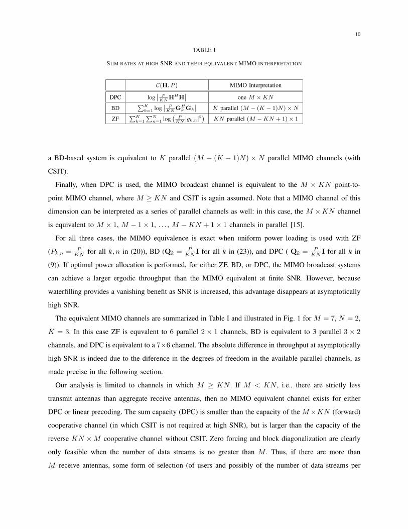
TABLE I

SUM RATES AT HIGH SNR AND THEIR EQUIVALENT MIMO INTERPRETATION

C(H, P ) MIMO Interpretation

DPC log˛

PKN

HHH˛

one M ×KN

BDPK

k=1 log˛

PKN

GHk Gk

˛K parallel (M − (K − 1)N)×N

ZFPK

k=1

PNn=1 log

`P

KN|gk,n|2

´KN parallel (M −KN + 1)× 1

a BD-based system is equivalent to K parallel (M − (K − 1)N) × N parallel MIMO channels (with

CSIT).

Finally, when DPC is used, the MIMO broadcast channel is equivalent to the M × KN point-to-

point MIMO channel, where M ≥ KN and CSIT is again assumed. Note that a MIMO channel of this

dimension can be interpreted as a series of parallel channels as well: in this case, the M ×KN channel

is equivalent to M × 1, M − 1× 1, . . . , M −KN + 1× 1 channels in parallel [15].

For all three cases, the MIMO equivalence is exact when uniform power loading is used with ZF

(Pk,n = PKN for all k, n in (20)), BD (Qk = P

KN I for all k in (23)), and DPC ( Qk = PKN I for all k in

(9)). If optimal power allocation is performed, for either ZF, BD, or DPC, the MIMO broadcast systems

can achieve a larger ergodic throughput than the MIMO equivalent at finite SNR. However, because

waterfilling provides a vanishing benefit as SNR is increased, this advantage disappears at asymptotically

high SNR.

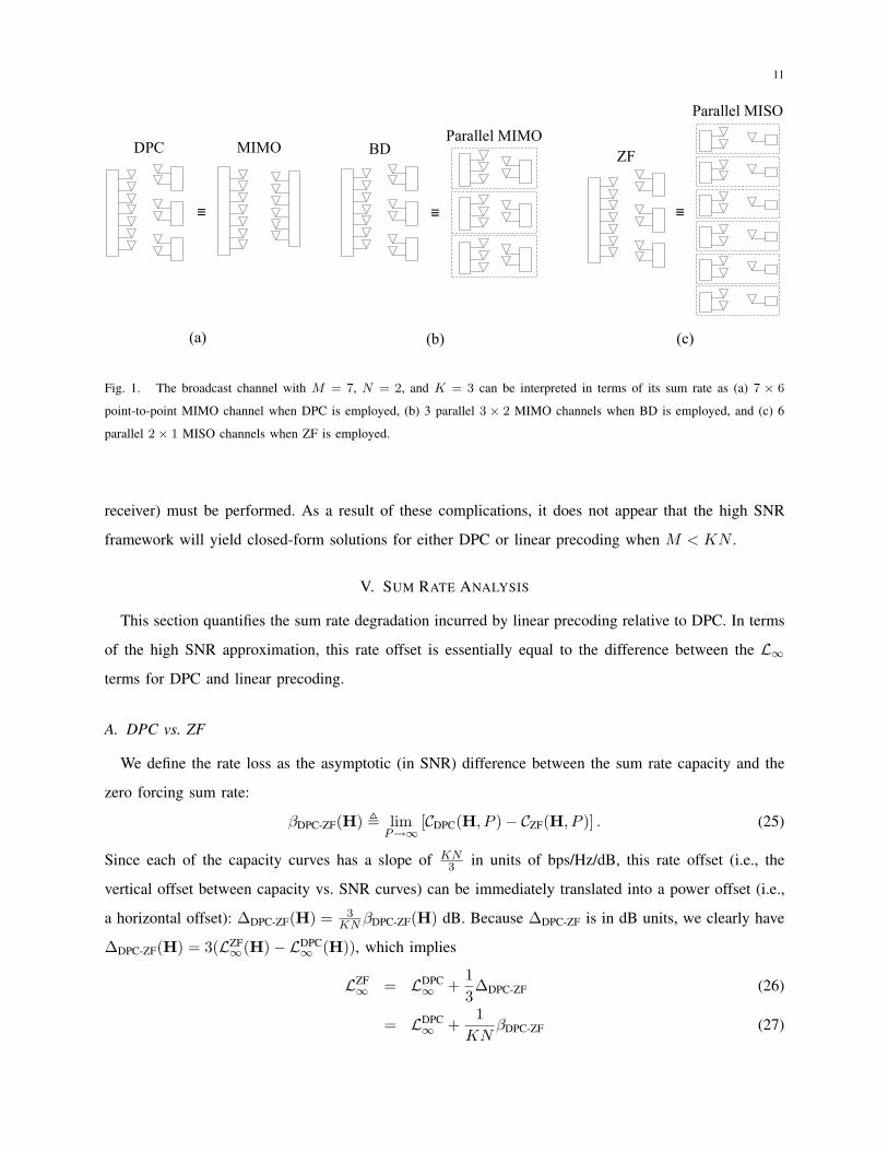
The equivalent MIMO channels are summarized in Table I and illustrated in Fig. 1 for M = 7, N = 2,

K = 3. In this case ZF is equvalent to 6 parallel 2 × 1 channels, BD is equivalent to 3 parallel 3 × 2

channels, and DPC is equivalent to a 7×6 channel. The absolute difference in throughput at asymptotically

high SNR is indeed due to the diference in the degrees of freedom in the available parallel channels, as

made precise in the following section.

Our analysis is limited to channels in which M ≥ KN . If M < KN , i.e., there are strictly less

transmit antennas than aggregate receive antennas, then no MIMO equivalent channel exists for either

DPC or linear precoding. The sum capacity (DPC) is smaller than the capacity of the M×KN (forward)

cooperative channel (in which CSIT is not required at high SNR), but is larger than the capacity of the

reverse KN ×M cooperative channel without CSIT. Zero forcing and block diagonalization are clearly

only feasible when the number of data streams is no greater than M . Thus, if there are more than

M receive antennas, some form of selection (of users and possibly of the number of data streams per

11

DPC

≡

MIMO

≡ ≡

BDParallel MIMO

ZF

Parallel MISO

(a) (b) (c)

Fig. 1. The broadcast channel with M = 7, N = 2, and K = 3 can be interpreted in terms of its sum rate as (a) 7 × 6

point-to-point MIMO channel when DPC is employed, (b) 3 parallel 3 × 2 MIMO channels when BD is employed, and (c) 6

parallel 2× 1 MISO channels when ZF is employed.

receiver) must be performed. As a result of these complications, it does not appear that the high SNR

framework will yield closed-form solutions for either DPC or linear precoding when M < KN .

V. SUM RATE ANALYSIS

This section quantifies the sum rate degradation incurred by linear precoding relative to DPC. In terms

of the high SNR approximation, this rate offset is essentially equal to the difference between the L∞terms for DPC and linear precoding.

A. DPC vs. ZF

We define the rate loss as the asymptotic (in SNR) difference between the sum rate capacity and the

zero forcing sum rate:

βDPC-ZF(H) , limP→∞

[CDPC(H, P )− CZF(H, P )] . (25)

Since each of the capacity curves has a slope of KN3 in units of bps/Hz/dB, this rate offset (i.e., the

vertical offset between capacity vs. SNR curves) can be immediately translated into a power offset (i.e.,

a horizontal offset): ∆DPC-ZF(H) = 3KN βDPC-ZF(H) dB. Because ∆DPC-ZF is in dB units, we clearly have

∆DPC-ZF(H) = 3(LZF∞(H)− LDPC∞ (H)), which implies

LZF∞ = LDPC

∞ +13∆DPC-ZF (26)

= LDPC∞ +

1KN

βDPC-ZF (27)

12

From the affine approximation to DPC and ZF sum rate found in (12) and (21), the rate loss incurred

by ZF is:

βDPC-ZF(H) = log2

|HHH|∏Kk=1

∏Nn=1 |gk,n|2

. (28)

While the above metric is the rate loss per realization, we are more interested in the average rate offset

across the fading distribution:

βDPC-ZF = EH [βDPC-ZF(H)] , (29)

which allows a comparison of ergodic (over the fading distribution) throughput. Likewise, the average

power offset is denoted as ∆DPC-ZF and can be immediately calculated in the same fashion. Under iid

Rayleigh fading, the matrix HHH is Wishart with 2M degrees of freedom while |gk,n|2 are identically

χ22(M−KN+1), as explained in Section IV-C.

The key to computing the average offset is the following closed form expression for the expectation

of the log determinant of a Wishart matrix:

Lemma 1 (Theorem 2.11 of [16]): If m × m matrix HHH is complex Wishart distributed with n

(≥ m) degrees of freedom (d.o.f), then:

E[loge

∣∣HHH∣∣]

=m−1∑

l=0

ψ(n− l), (30)

where ψ(·) is Euler’s digamma function, which satisifes

ψ(m) = ψ(1) +m−1∑

l=1

1l

(31)

for positive integers m and ψ(1) ≈ −0.577215.

This result can be directly applied to chi-squared random variables by noting that a 1×1 complex Wishart

matrix with n degrees of freedom is χ22n:

E [loge χ22n] = ψ(n). (32)

Using Lemma 1 we can compute the average rate offset in closed form:

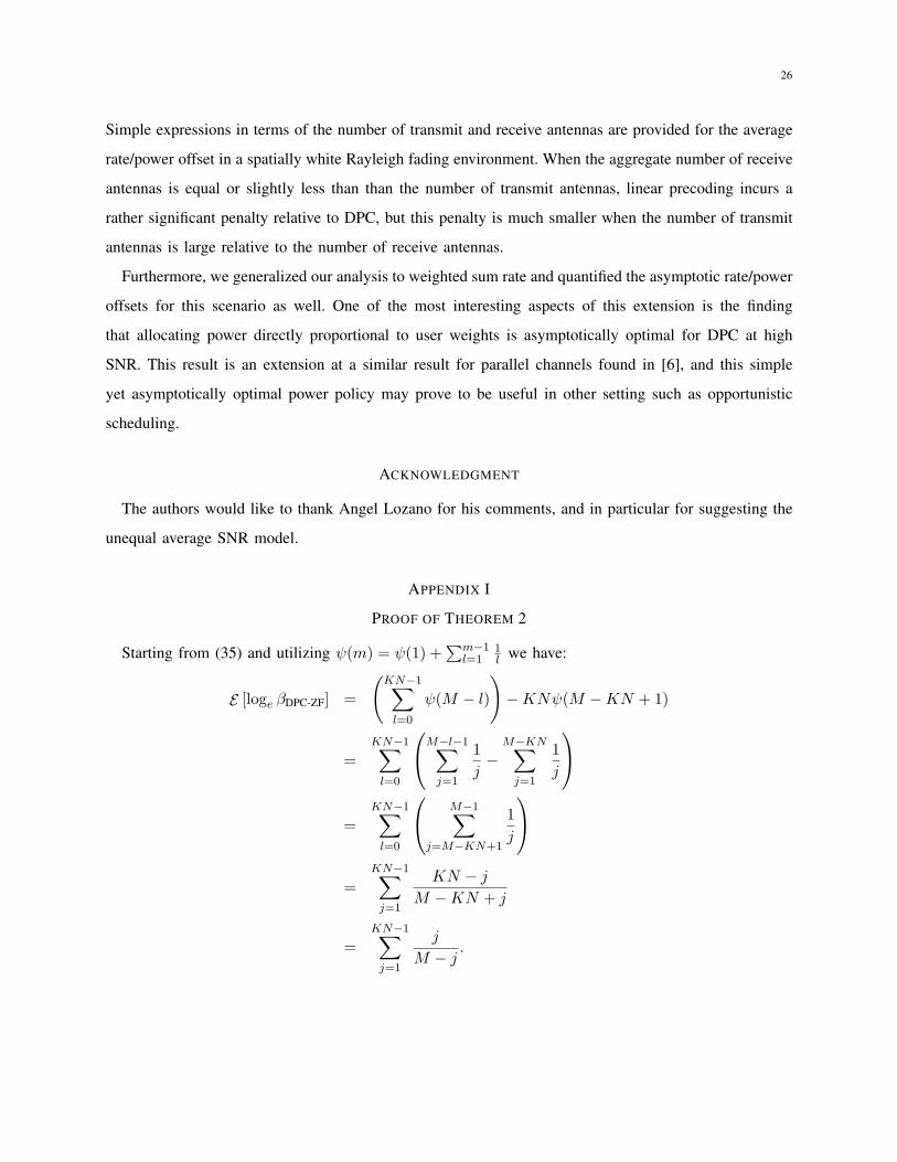
Theorem 2: The expected loss in Rayleigh fading due to zero-forcing is given by

βDPC-ZF(M, KN) = log2 eKN−1∑

j=1

j

M − j(bps/Hz). (33)

13

Proof: Since HHH is KN ×KN Wishart with M d.o.f, and |gk,n|2 is χ22(M−KN+1), Lemma 1

applied to (29) gives:

βDPC-ZF = E[loge |HHH|]−KN · E

[loge |g1,1|2

](34)

= log2 e

[(KN−1∑

l=0

ψ(M − l)

)−KNψ(M −KN + 1)

](35)

By expanding the digamma function and performing the algebraic manipulations shown in Appendix I,

the form (33) can be reached.

Using this result we easily get an expression for the rate offset LZF∞(M,KN) by plugging into (27)

LZF∞(M, KN) = LDPC

∞ (M, KN) +1

KNβDPC-ZF(M,KN) (36)

= LMIMO∞ (KN, M) +

log2 e

KN

KN−1∑

j=1

j

M − j, (37)

where LMIMO∞ (KN,M) is the rate offset of a KN transmit antenna, M receive antenna MIMO channel

in iid Rayleigh fading, which is defined in Proposition 1 of [7].

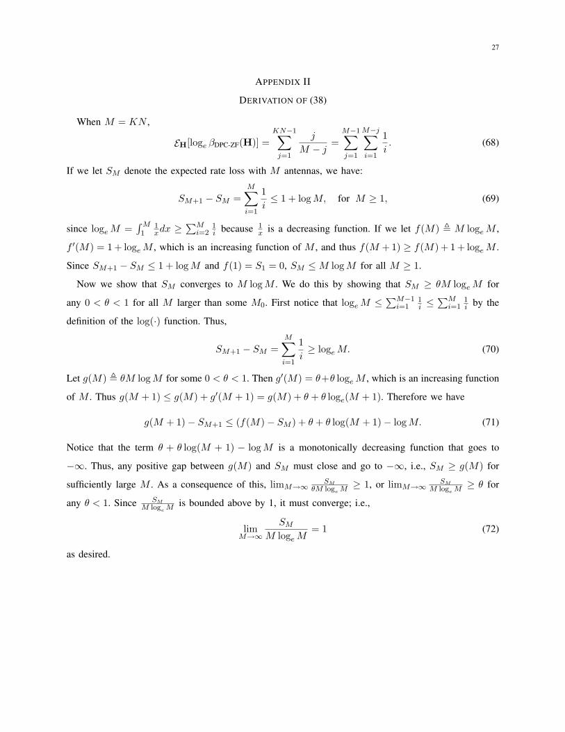
When the total number of receive antennas is equal to M (i.e., M = KN ), ZF incurs a rather large

loss relative to DPC that can be approximated as:

βDPC-ZF(M) ≈ M log2 M (bps/Hz) (38)

in the sense that the ratio of both sides converges to one as M grows large (see Appendix II for the

proof). In this scenario, the ZF sum rate is associated with the capacity of M parallel 1 × 1 (SISO)

channels while the DPC sum rate is associated with a M ×M MIMO channel. This corresponds to a

power offset of 3 log2 M (dB), which is very significant when M is large. Note that the approximation

3 log2 M (dB) overstates the power penalty by 1 to 1.5 dB for reasonable values of M(< 20), but does

capture the growth rate. Such a large penalty is not surprising, since the use of zero-forcing requires

inverting the M ×M matrix H, which is poorly conditioned with high probability when M is large.

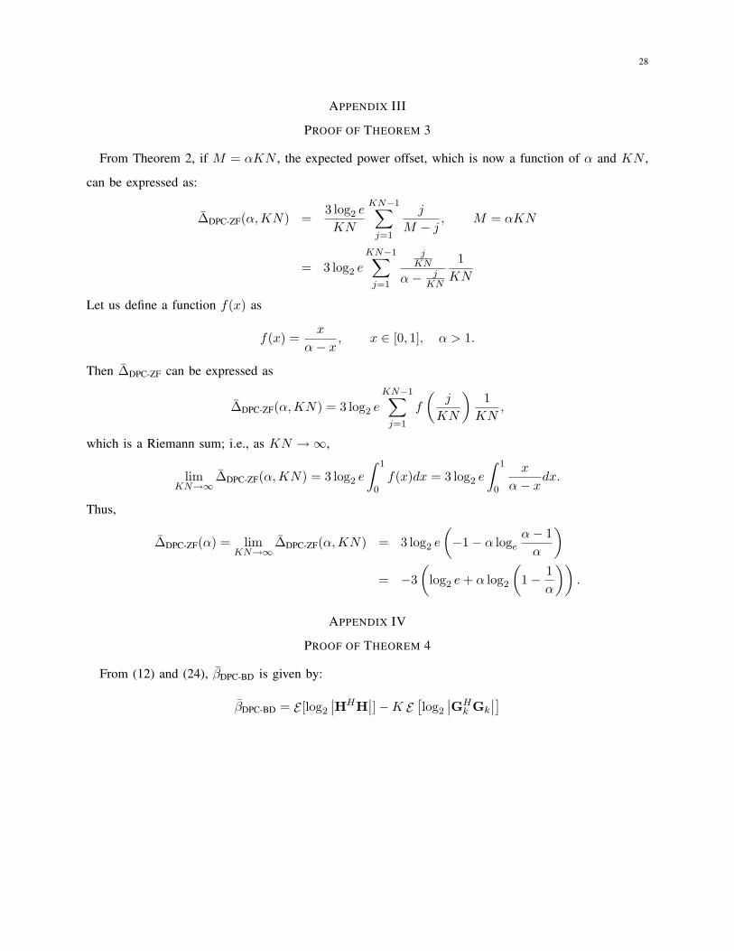
We can also consider the asymptotic ZF penalty when the number of transmit antennas is much larger

than the number of receive antennas. If the number of users and transmit antennas are taken to infinity

at a fixed ratio according to M = αKN with KN →∞ for some α > 1, then the power offset between

DPC and ZF converges to a constant:

Theorem 3: For M = αKN with α > 1, KN → ∞, the asymptotic power penalty for ZF is given

by

∆DPC-ZF(α) = −3(

log2 e + α log2

(1− 1

α

))(dB). (39)

14

Proof: See Appendix III.

This power offset is incurred due to the fact that the DPC sum rate increases according to a KN×αKN

MIMO channel capacity while the ZF sum rate increases according to KN parallel (α − 1)KN × 1

MISO channels. For example, if α = 2, or the number of transmit antennas is double the number of

receivers, the zero-forcing penalty is no larger than 1.67 dB, and monotonic convergence to this asymptote

is observed. Thus for large systems, ZF is a viable low-complexity alternative to DPC if the number of

transmit antennas can be made suitably large. A similar conclusion was drawn in [17] where the ratio of

the rates achievable with ZF relative to the sum capacity is studied. Note that using ZF on the MIMO

downlink channel is identical to using a decorrelating receiver on the multiple antenna uplink channel or

in a randomly spread CDMA system; as a result Theorem 3 is identical to the asymptotic performance

of the decorrelating CDMA receiver given in Eq. (152) of [3].

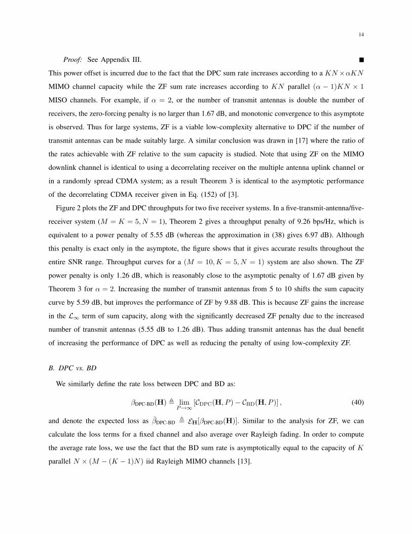
Figure 2 plots the ZF and DPC throughputs for two five receiver systems. In a five-transmit-antenna/five-

receiver system (M = K = 5, N = 1), Theorem 2 gives a throughput penalty of 9.26 bps/Hz, which is

equivalent to a power penalty of 5.55 dB (whereas the approximation in (38) gives 6.97 dB). Although

this penalty is exact only in the asymptote, the figure shows that it gives accurate results throughout the

entire SNR range. Throughput curves for a (M = 10,K = 5, N = 1) system are also shown. The ZF

power penalty is only 1.26 dB, which is reasonably close to the asymptotic penalty of 1.67 dB given by

Theorem 3 for α = 2. Increasing the number of transmit antennas from 5 to 10 shifts the sum capacity

curve by 5.59 dB, but improves the performance of ZF by 9.88 dB. This is because ZF gains the increase

in the L∞ term of sum capacity, along with the significantly decreased ZF penalty due to the increased

number of transmit antennas (5.55 dB to 1.26 dB). Thus adding transmit antennas has the dual benefit

of increasing the performance of DPC as well as reducing the penalty of using low-complexity ZF.

B. DPC vs. BD

We similarly define the rate loss between DPC and BD as:

βDPC-BD(H) , limP→∞

[CDPC(H, P )− CBD(H, P )] , (40)

and denote the expected loss as βDPC-BD , EH[βDPC-BD(H)]. Similar to the analysis for ZF, we can

calculate the loss terms for a fixed channel and also average over Rayleigh fading. In order to compute

the average rate loss, we use the fact that the BD sum rate is asymptotically equal to the capacity of K

parallel N × (M − (K − 1)N) iid Rayleigh MIMO channels [13].

15

0 5 10 15 20 25 300

5

10

15

20

25

30

35

40

45

50

SNR (dB)

Cap

acity

(bp

s/H

z)

Sum Rate vs. SNR

M=5, K=5

ZF

DPC

M=10, K=5

DPCZF

5.55 dB

9.88 dB

Fig. 2. DPC vs. zero-forcing at high SNR

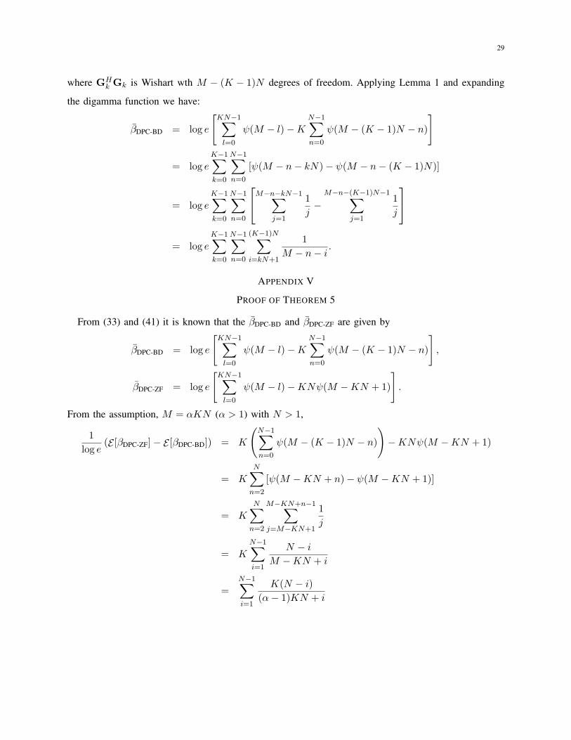
Theorem 4: The expected loss in Rayleigh fading due to block diagonalization is given by

βDPC-BD(M, K, N) = (log2 e)

K−1∑

k=0

N−1∑

n=0

(K−1)N∑

i=kN+1

1M − n− i

(bps/Hz). (41)

Proof: See Appendix IV.

Eq. (41) simplifies to (33) when N = 1; i.e., zero-forcing is a special case of block diagonalization. If

the number of transmit antennas M is kept fixed but N is increased and K is decreased such that KN

is constant, i.e., the number of antennas per receiver is increased but the aggregate number of receive

antennas is kept constant, then the rate offset decreases. In the degenerate case M = N and K = 1 the

channel becomes a point-to-point MIMO channel and the offset is indeed zero. Using the same procedure

as for ZF, we can easily get an expression for the rate offset LBD∞ (M, K, N) (27)

LBD∞ (M, K,N) = LMIMO

∞ (KN, M) +1

KNβDPC-BD(M,N, K). (42)

Although it is difficult to obtain insight directly from Theorem 4, it is much more useful to consider

the offset between BD (K receivers with N antennas each) and ZF (equivalent to KN receivers with 1

antenna each).

Theorem 5: If M = αKN with N > 1 and α > 1, the expected throughput gain of BD relative to

16

ZF is:

βBD-ZF , βDPC-ZF(M, NK)− βDPC-BD(M, N, K)

= (log2 e)KN−1∑

j=1

(N − j)(α− 1)KN + j

(bps/Hz)

=3 log2 e

N

N−1∑

j=1

(N − j)(α− 1)KN + j

(dB).

Proof: See Appendix V.

A direct corollary of this is an expression for the expected power offset when M = KN :

∆BD-ZF(N) =3(log2 e)

N

N−1∑

j=1

N − j

j(dB). (43)

Note that this expression only depends on the number of receive antennas per receiver and is independent

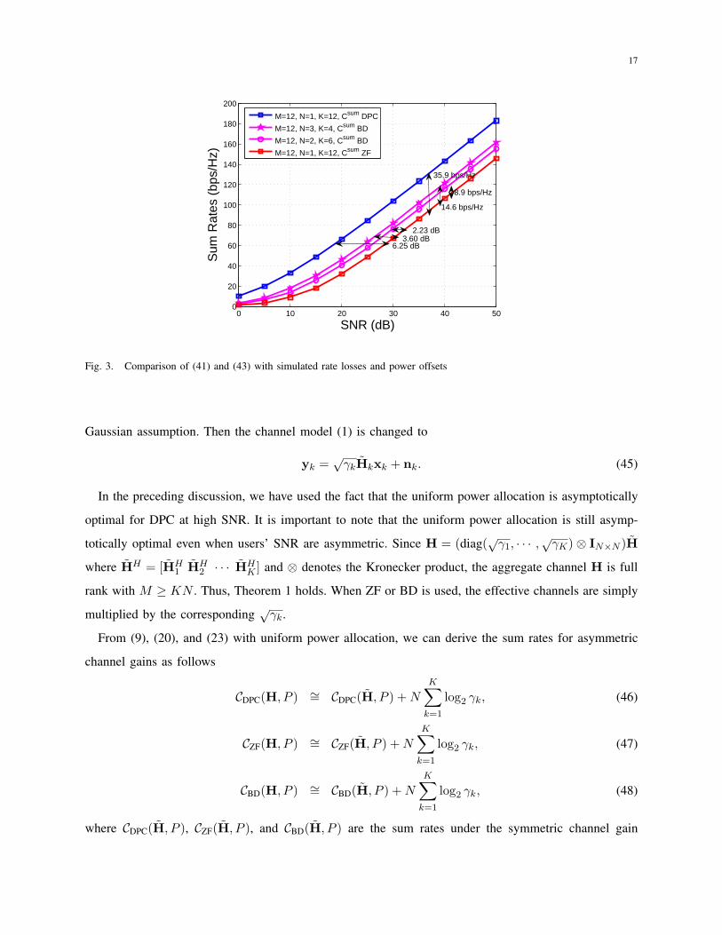
of the number of users, i.e., of the system size. For example, consider two system configurations: (i) M2

receivers each have two antennas, and (ii) M receivers each have one antenna. Equation (43) indicates that

the power advantage of using BD in the N = 2 system is ∆BD-ZF = 2.1640 (dB) relative to performing

ZF. Since this offset is independent of M , it is the same for M = 4 and K = 4, N = 1 vs. K = 2, N = 2

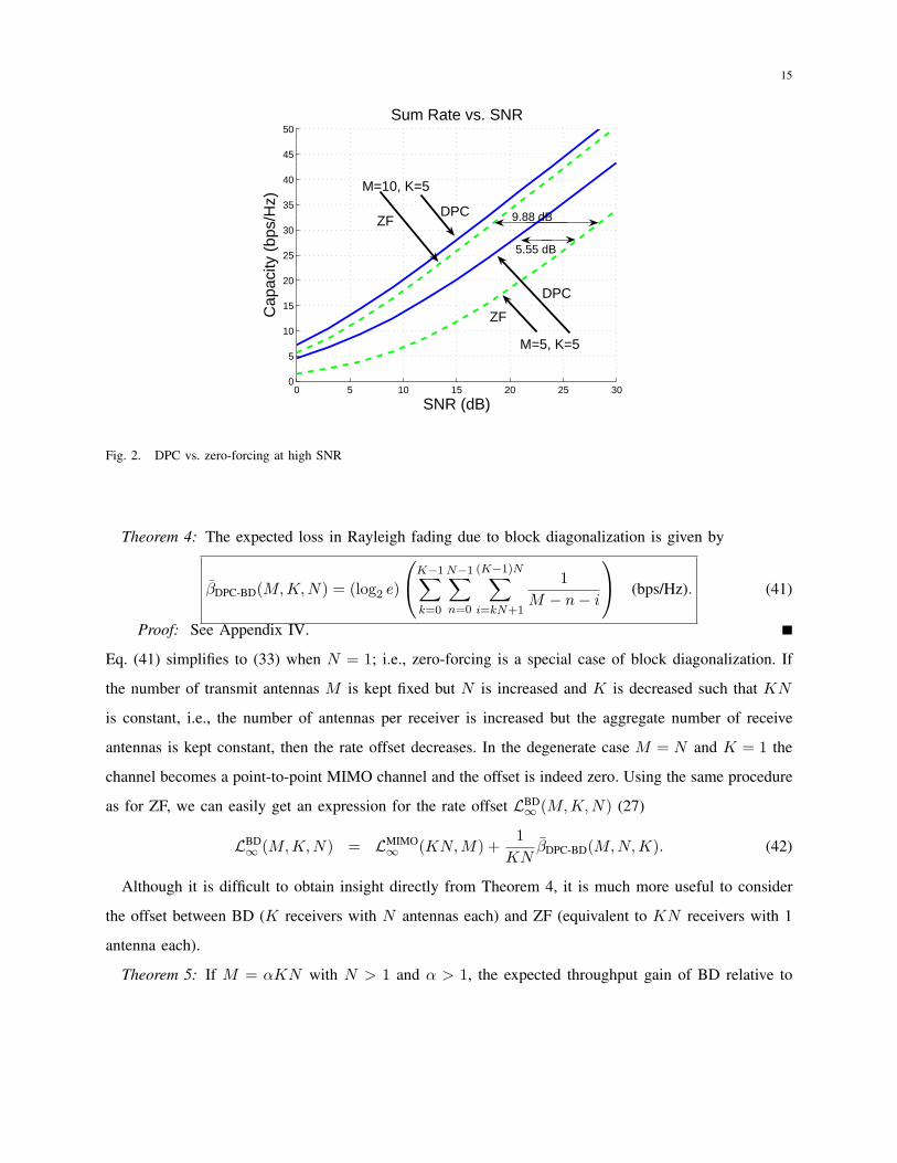
systems as well as for M = 6 and K = 6, N = 1 vs. K = 3, N = 2 systems. To illustrate the utility of

the asymptotic rate offsets, sum rates are plotted in Fig. 3 for systems with M = 12 and N = 3, K = 4,

and N = 2, K = 6. Notice that the asymptotic offsets provide insight at even moderate SNR levels (e.g.,

10 dB). When M = 12, N = 3, K = 4, βBD-ZF = 14.4270 (bps/Hz) and ∆BD-ZF = 3.6067 (dB) while

the numerical values are 14.6 (bps/Hz) and 3.65 (dB), respectively.

C. Unequal Average SNR’s

The underlying assumption beforehand is that the strengths of channel gains are the same for all

users. However, there exist near-far effects in a typical wireless broadcast channel scenario which lead

to asymmetric channel gains. In this subsection, we consider the effect of asymmetric channel gains or

unequal average SNR and reformulate the rate offsets (33) and (41).

We assume that the channel gain of each user can be decomposed into

Hk =√

γkHk, k = 1, · · · ,K, (44)

where γk denotes the average SNR of user k. The elements of Hk have Gaussian distribution with

mean zero and unit variance. Notice that the quantities with tilde (·) are derived under a zero mean unit

17

0 10 20 30 40 500

20

40

60

80

100

120

140

160

180

200

SNR (dB)

Sum

Rat

es (

bps/

Hz)

M=12, N=1, K=12, Csum DPC

M=12, N=3, K=4, Csum BD

M=12, N=2, K=6, Csum BD

M=12, N=1, K=12, Csum ZF

8.9 bps/Hz

14.6 bps/Hz

35.9 bps/Hz

2.23 dB3.60 dB

6.25 dB

Fig. 3. Comparison of (41) and (43) with simulated rate losses and power offsets

Gaussian assumption. Then the channel model (1) is changed to

yk =√

γkHkxk + nk. (45)

In the preceding discussion, we have used the fact that the uniform power allocation is asymptotically

optimal for DPC at high SNR. It is important to note that the uniform power allocation is still asymp-

totically optimal even when users’ SNR are asymmetric. Since H = (diag(√

γ1, · · · ,√

γK)⊗ IN×N )H

where HH = [HH1 HH

2 · · · HHK ] and ⊗ denotes the Kronecker product, the aggregate channel H is full

rank with M ≥ KN . Thus, Theorem 1 holds. When ZF or BD is used, the effective channels are simply

multiplied by the corresponding√

γk.

From (9), (20), and (23) with uniform power allocation, we can derive the sum rates for asymmetric

channel gains as follows

CDPC(H, P ) ∼= CDPC(H, P ) + N

K∑

k=1

log2 γk, (46)

CZF(H, P ) ∼= CZF(H, P ) + NK∑

k=1

log2 γk, (47)

CBD(H, P ) ∼= CBD(H, P ) + NK∑

k=1

log2 γk, (48)

where CDPC(H, P ), CZF(H, P ), and CBD(H, P ) are the sum rates under the symmetric channel gain

18

0 5 10 15 20 25 30 35 400

5

10

15

20

25

30

35

40

45

SNR (dB)

Sum

Rat

es

DPC with Optimal Power AllocationDPC with Uniform Power AllocationZF with Optimal Power AllocationZF with Uniform Power Allocation

Fig. 4. Average sum rates with the optimal power allocation and the uniform power allocation when M = 4, N = 1, K = 4,

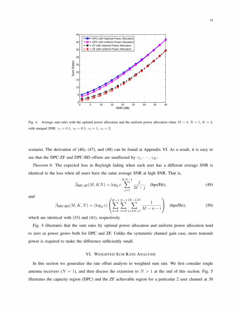
with unequal SNR: γ1 = 0.1, γ2 = 0.5, γ3 = 1, γ4 = 2.

scenario. The derivation of (46), (47), and (48) can be found at Appendix VI. As a result, it is easy to

see that the DPC-ZF and DPC-BD offsets are unaffected by γ1, · · · , γK :

Theorem 6: The expected loss in Rayleigh fading when each user has a different average SNR is

identical to the loss when all users have the same average SNR at high SNR. That is,

βDPC-ZF(M, KN) = log2 eKN−1∑

j=1

j

M − j(bps/Hz), (49)

and

βDPC-BD(M, K, N) = (log2 e)

K−1∑

k=0

N−1∑

n=0

(K−1)N∑

i=kN+1

1M − n− i

(bps/Hz), (50)

which are identical with (33) and (41), respectively.

Fig. 4 illustrates that the sum rates by optimal power allocation and uniform power allocation tend

to zero as power grows both for DPC and ZF. Unlike the symmetric channel gain case, more transmit

power is required to make the difference sufficiently small.

VI. WEIGHTED SUM RATE ANALYSIS

In this section we generalize the rate offset analysis to weighted sum rate. We first consider single

antenna receivers (N = 1), and then discuss the extension to N > 1 at the end of this section. Fig. 5

illustrates the capacity region (DPC) and the ZF achievable region for a particular 2 user channel at 30

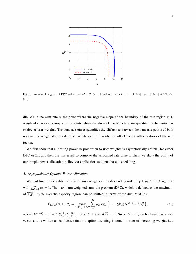
19

0 2 4 6 8 10 120

2

4

6

8

10

12

R1

R2

DPC Region

ZF Region

Fig. 5. Achievable regions of DPC and ZF for M = 2, N = 1, and K = 2, with h1 = [1 0.5], h2 = [0.5 1] at SNR=30

(dB).

dB. While the sum rate is the point where the negative slope of the boundary of the rate region is 1,

weighted sum rate corresponds to points where the slope of the boundary are specified by the particular

choice of user weights. The sum rate offset quantifies the difference between the sum rate points of both

regions; the weighted sum rate offset is intended to describe the offset for the other portions of the rate

region.

We first show that allocating power in proportion to user weights is asymptotically optimal for either

DPC or ZF, and then use this result to compute the associated rate offsets. Then, we show the utility of

our simple power allocation policy via application to queue-based scheduling.

A. Asymptotically Optimal Power Allocation

Without loss of generality, we assume user weights are in descending order: µ1 ≥ µ2 ≥ · · · ≥ µK ≥ 0

with∑K

k=1 µk = 1. The maximum weighted sum rate problem (DPC), which is defined as the maximum

of∑K

k=1 µkRk over the capacity region, can be written in terms of the dual MAC as:

CDPC(µ,H, P ) = maxPKk=1 Pk≤P

K∑

k=1

µk log2

(1 + Pkhk(A(k−1))−1hH

k

), (51)

where A(k−1) = I +∑k−1

j=1 PjhHj hj for k ≥ 1 and A(0) = I. Since N = 1, each channel is a row

vector and is written as hk. Notice that the uplink decoding is done in order of increasing weight, i.e.,

20

user K does not get the benefit of any interference cancellation while user 1’s signal benefits from full

interference cancellation and is thus detected in the presence of only noise.

The following lemma shows that if we limit ourselves to linear power allocation policies of the form

Pk = αkP , then the objective function in (51) can be decoupled at high SNR:

Lemma 2: If M ≥ K, then for any αk > 0, k = 1, · · · ,K with∑K

k=1 αk = 1,

limP→∞

[K∑

k=1

µk log2

(1 + αkPhk(A(k−1))−1hH

k

)−

K∑

k=1

µk log2

(1 + αkP‖fk‖2

)]

= 0, (52)

where fk is the projection of hk onto the nullspace of {h1, · · · ,hk−1}.

Proof: Lemma 3 in Appendix VII shows that hk(A(k−1))−1hHk → ‖fk‖2 as P → ∞. By the

continuity of log(·) and the fact that P →∞, we get the result.

Once the weighted sum rate maximization has been decoupled into the problem of maximizing weighted

sum rate over parallel single-user channels, we can use the result of [6] to show that the optimal power

allocation is of the form P ∗k = µkP + O(1).

Theorem 7: When M ≥ K, allocating power according to

Pk = µkP, k = 1, · · · ,K (53)

asymptotically achieves the optimal solution to (51) at high SNR.

Proof: By Lemma 2, the following optimization will yield an asymptotically optimal solution (albeit

with a weak restriction on allowable power policies):

maxPk:

PKk=1 Pk≤P

K∑

k=1

µk log2

(1 + Pk‖fk‖2

). (54)

The optimal power policy for a more general version of this problem, in which there are more than K

parallel channels and each user can occupy multiple channels, is solved in [6]. We need only consider

this simplified version, and it is easily checked (via KKT conditions) that the solution to (54) is:

P ∗k = µkP + µk

(∑

i

1‖fi‖2

)− 1‖fk‖2

, for k = 1, · · · ,K, (55)

when P is sufficiently large to allow all users to have non-zero power. Therefore, at high SNR we have

P ∗k = µkP + O(1), k = 1, · · · ,K. (56)

Since the O(1) power term leads to a vanishing rate, we have the result.

Theorem 7 generalizes the fact that uniform power allocation achieves the maximum sum rate asymptot-

ically at high SNR. That is, for the sum rate problem the weights are the same (i.e., µ1 = · · · = µK =

1/K), thus the uniform power policy is asymptotically optimal.

21

0 5 10 15 20 25 30−0.005

0

0.005

0.01

0.015

0.02

0.025

0.03

Mea

n E

rror

(bp

s/H

z)

SNR (dB)

Fig. 6. Averaged weighted sum rate difference between the exact solution (51) and the asymptotic solution (53) when µ1 = 0.6

and µ2 = 0.4 for Rayleigh fading channel.

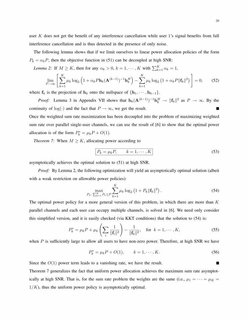
In Fig. 6 the difference between the true weighted sum rate (51) and the weighted sum rate achieved

using Pk = µkP is plotted as a function of SNR. This difference is averaged over iid Rayleigh channel

realizations for a (M = 4,K = 2, N = 1) system with µ1 = 0.6 and µ2 = 0.4. The approximate power

allocation is seen to give a weighted sum rate that is extremely close to the optimum even at very low

SNR values.

Meanwhile, the weighted sum rate by ZF is given by

CZF(µ,H, P ) = maxPk:

PKk=1 Pk≤P

K∑

k=1

µk log2

(1 + Pk‖gk‖2

), (57)

where gk is the projection of hk onto the null space of {h1, · · · ,hk−1,hk+1, · · · ,hK}. The result of [6]

directly applies here, and therefore the power allocation policy in (53) is also the asymptotic solution to

(57).

22

Resource

Allocation

1λ

2λ

1( )q t

2( )q t

...

M

User 1

User 2

Fig. 7. MIMO BC with queues

B. Rate Loss

Using the asymptotically optimal power allocation policy of (53), the weighted sum rates of DPC and

ZF can be expressed as

CDPC(µ,H, P ) ∼=K∑

k=1

µk log(1 + µkP‖fk‖2

), (58)

CZF(µ,H, P ) ∼=K∑

k=1

µk log(1 + µkP‖gk‖2

). (59)

Thus, the rate offset per realization is given by

βDPC-ZF(µ,H) ∼=K∑

k=1

µk log‖fk‖2

‖gk‖2. (60)

In Rayleigh fading, the distributions of ‖fk‖2 and ‖gk‖2 are χ22(M−k+1) and χ2

2(M−K+1), respectively.

Therefore, the expected rate loss is given by

βDPC-ZF(µ,M,K) ∼= (log2 e)K∑

k=1

µk

M−k∑

j=M−K+1

1j

. (61)

It is straightforward to check that the rate offset is minimized at the sum rate, i.e., when µ1 = · · · =µk = 1

K . If we let ζk =∑M−k

j=M−K+11j , then ζ1 > ζ2 > · · · > ζK and βDPC-ZF = (log2 e)

∑Kk=1 µkζk.

Since {µk} has constraints of µ1 ≥ · · · ≥ µK ,∑K

k=1 µ1 = 1, and µk ≥ 0 (1 ≤ k ≤ K), βDPC-ZF achieves

minimum at µ1 = · · · = µk = 1K for a given {ζk}.

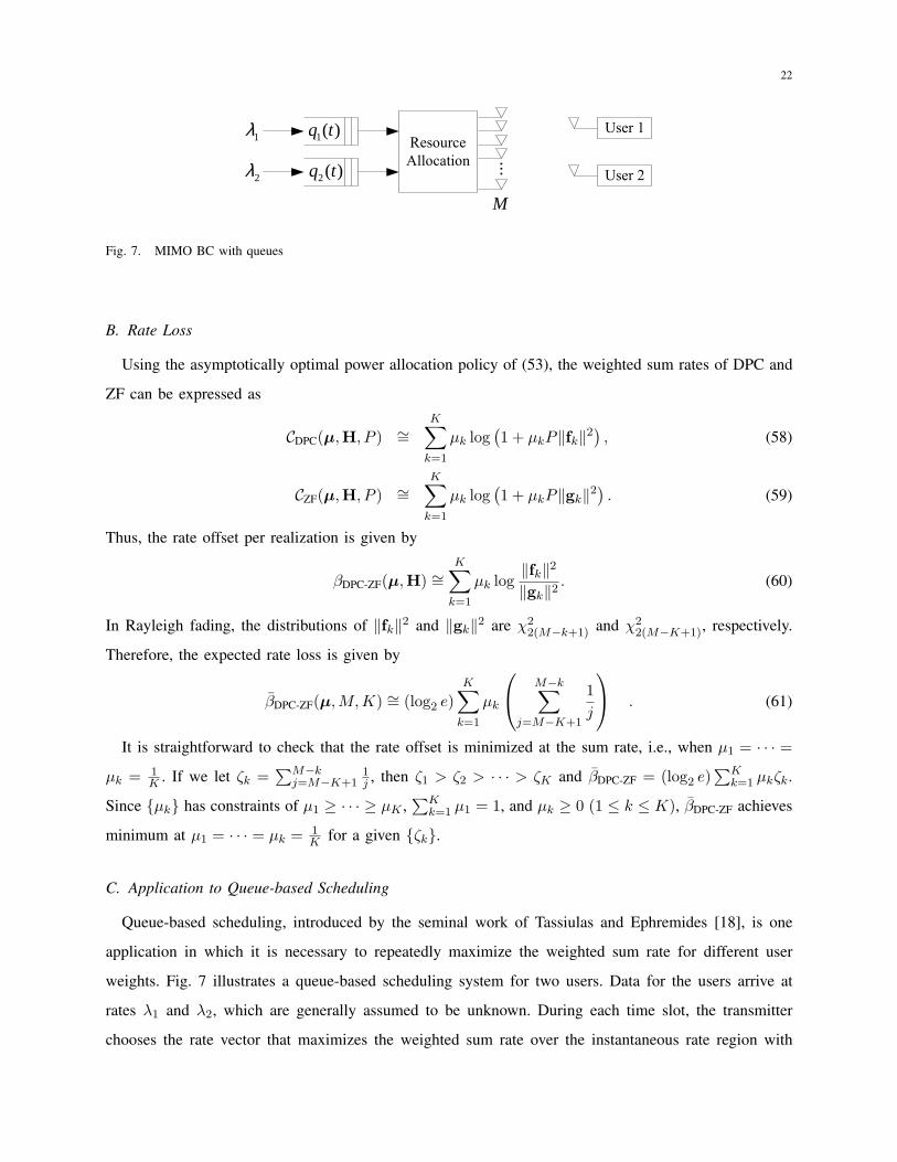
C. Application to Queue-based Scheduling

Queue-based scheduling, introduced by the seminal work of Tassiulas and Ephremides [18], is one

application in which it is necessary to repeatedly maximize the weighted sum rate for different user

weights. Fig. 7 illustrates a queue-based scheduling system for two users. Data for the users arrive at

rates λ1 and λ2, which are generally assumed to be unknown. During each time slot, the transmitter

chooses the rate vector that maximizes the weighted sum rate over the instantaneous rate region with

23

weights equal to the current queue sizes. If the queue lengths are denoted as q1(t) and q2(t), then the

transmitter solves the following optimization during each time slot:

maxR∈C(H,P )

q1(t)R1 + q2(t)R2, (62)

and such a policy stabilizes any rate vector in the ergodic capacity region.

Although the weighted sum rate maximization problem for DPC stated in equation (51) is convex,

it still requires considerable complexity and could be difficult to perform on a slot-by-slot basis. An

alternative is to use the approximate power allocation policy from (53) during each time slot:

Pk =qk(t)

q1(t) + q2(t)P, (63)

and where the ordering of the queues determines the dual MAC decoding order (larger queue decoded

last).

Although we do not yet have any analytical results on the performance of the asymptotically optimal

power policy, numerical results indicate that such a policy performs nearly as well as actually maximizing

weighted sum rate. Ongoing work is investigating whether the approximate strategy is stabilizing for this

system.

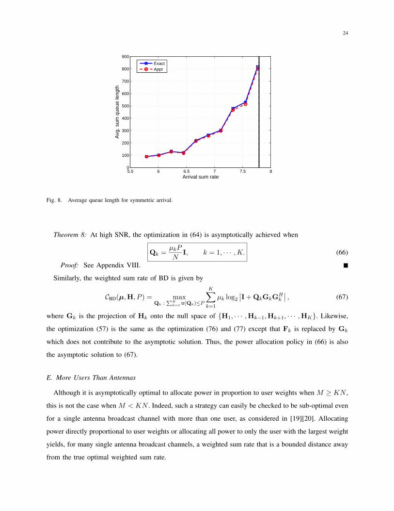
In Fig. 8 average queue length is plotted versus the sum arrival rate for an M = 4, K = 2 channel at

10 dB, for both the exact weighted sum rate maximization as well as the approximation. Both schemes

are seen to perform nearly identical, and the approximate algorithm appears to stabilize the system in

this scenario, although this is only empirical evidence.

D. Extension to N > 1

Similar to (51), the weighted sum rate by DPC can be as:

CDPC(µ,H, P ) = maxPKk=1 tr(Qk)≤P

K∑

k=1

µk log2

|A(k)||A(k−1)| , (64)

where A(k) = I +∑k

j=1 HHj QjHj for k ≥ 1 and A(0) = I. From the construction of A(k),

|A(k)||A(k−1)| =

∣∣∣I + QkHk(A(k−1))−1HHk

∣∣∣ .

Hence, (64) can be written as

CBC(µ,H, P ) = maxPKk=1 tr(Qk)≤P

K∑

k=1

µk log2

∣∣∣I + QkHk(A(k−1))−1HHk

∣∣∣ . (65)

With the decoupling lemma (see Appendix VII), the above optimization (65) can be solved asymptotically

like the case of N = 1:

24

5.5 6 6.5 7 7.5 80

100

200

300

400

500

600

700

800

900

Arrival sum rate

Avg

. sum

que

ue le

ngth

ExactAppr

Fig. 8. Average queue length for symmetric arrival.

Theorem 8: At high SNR, the optimization in (64) is asymptotically achieved when

Qk =µkP

NI, k = 1, · · · ,K. (66)

Proof: See Appendix VIII.

Similarly, the weighted sum rate of BD is given by

CBD(µ,H, P ) = maxQk :

PKk=1 tr(Qk)≤P

K∑

k=1

µk log2

∣∣I + QkGkGHk

∣∣ , (67)

where Gk is the projection of Hk onto the null space of {H1, · · · ,Hk−1,Hk+1, · · · ,HK}. Likewise,

the optimization (57) is the same as the optimization (76) and (77) except that Fk is replaced by Gk

which does not contribute to the asymptotic solution. Thus, the power allocation policy in (66) is also

the asymptotic solution to (67).

E. More Users Than Antennas

Although it is asymptotically optimal to allocate power in proportion to user weights when M ≥ KN ,

this is not the case when M < KN . Indeed, such a strategy can easily be checked to be sub-optimal even

for a single antenna broadcast channel with more than one user, as considered in [19][20]. Allocating

power directly proportional to user weights or allocating all power to only the user with the largest weight

yields, for many single antenna broadcast channels, a weighted sum rate that is a bounded distance away

from the true optimal weighted sum rate.

25

0 5 10 15 20 25 30 35 40 45 500

2

4

6

8

10

12

14Optimal power allocationPower proportional to the weightsPower proportional to the relative weights to the first 2 users

0.09 bps/Hz

0.16 bps/Hz

SNR (dB)

Weighted Sum Rate

Fig. 9. Ergodic weighted sum rates by DPC and by approximations when M = 2, N = 1, K = 3, with µ1 = 0.5, µ2 = 0.3,

and µ3 = 0.2.

Although neither of these strategies is asymptotically optimal, numerical results do show that these

approximations achieve rates that are extremely close to optimum. In general, there are two different

reasonable power approximations. The first is to simply choose Pk = µkP . However, when K > M , this

results in sending many more data streams than there are spatial dimensions, which is not particularly

intuitive. An alternative strategy is to allocate power to the users with the M largest weights, but again

in proportion to their weights.

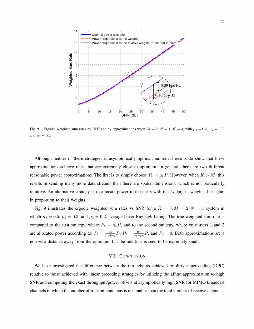
Fig. 9 illustrates the ergodic weighted sum rates vs SNR for a K = 3,M = 2, N = 1 system in

which µ1 = 0.5, µ2 = 0.3, and µ3 = 0.2, averaged over Rayleigh fading. The true weighted sum rate is

compared to the first strategy, where Pk = µkP , and to the second strategy, where only users 1 and 2

are allocated power according to: P1 = µ1

µ1+µ2P , P2 = µ2

µ1+µ2P , and P3 = 0. Both approximations are a

non-zero distance away from the optimum, but the rate loss is seen to be extremely small.

VII. CONCLUSION

We have investigated the difference between the throughputs achieved by dirty paper coding (DPC)

relative to those achieved with linear precoding strategies by utilizing the affine approximation to high

SNR and computing the exact throughput/power offsets at asymptotically high SNR for MIMO broadcast

channels in which the number of transmit antennas is no smaller than the total number of receive antennas.

26

Simple expressions in terms of the number of transmit and receive antennas are provided for the average

rate/power offset in a spatially white Rayleigh fading environment. When the aggregate number of receive

antennas is equal or slightly less than than the number of transmit antennas, linear precoding incurs a

rather significant penalty relative to DPC, but this penalty is much smaller when the number of transmit

antennas is large relative to the number of receive antennas.

Furthermore, we generalized our analysis to weighted sum rate and quantified the asymptotic rate/power

offsets for this scenario as well. One of the most interesting aspects of this extension is the finding

that allocating power directly proportional to user weights is asymptotically optimal for DPC at high

SNR. This result is an extension at a similar result for parallel channels found in [6], and this simple

yet asymptotically optimal power policy may prove to be useful in other setting such as opportunistic

scheduling.

ACKNOWLEDGMENT

The authors would like to thank Angel Lozano for his comments, and in particular for suggesting the

unequal average SNR model.

APPENDIX I

PROOF OF THEOREM 2

Starting from (35) and utilizing ψ(m) = ψ(1) +∑m−1

l=11l we have:

E [loge βDPC-ZF] =

(KN−1∑

l=0

ψ(M − l)

)−KNψ(M −KN + 1)

=KN−1∑

l=0

M−l−1∑

j=1

1j−

M−KN∑

j=1

1j

=KN−1∑

l=0

M−1∑

j=M−KN+1

1j

=KN−1∑

j=1

KN − j

M −KN + j

=KN−1∑

j=1

j

M − j.

27

APPENDIX II

DERIVATION OF (38)

When M = KN ,

EH[loge βDPC-ZF(H)] =KN−1∑

j=1

j

M − j=

M−1∑

j=1

M−j∑

i=1

1i. (68)

If we let SM denote the expected rate loss with M antennas, we have:

SM+1 − SM =M∑

i=1

1i≤ 1 + log M, for M ≥ 1, (69)

since loge M =∫ M1

1xdx ≥ ∑M

i=21i because 1

x is a decreasing function. If we let f(M) , M loge M ,

f ′(M) = 1 + loge M , which is an increasing function of M , and thus f(M + 1) ≥ f(M) + 1 + loge M .

Since SM+1 − SM ≤ 1 + log M and f(1) = S1 = 0, SM ≤ M log M for all M ≥ 1.

Now we show that SM converges to M log M . We do this by showing that SM ≥ θM loge M for

any 0 < θ < 1 for all M larger than some M0. First notice that loge M ≤ ∑M−1i=1

1i ≤

∑Mi=1

1i by the

definition of the log(·) function. Thus,

SM+1 − SM =M∑

i=1

1i≥ loge M. (70)

Let g(M) , θM log M for some 0 < θ < 1. Then g′(M) = θ+θ loge M , which is an increasing function

of M . Thus g(M + 1) ≤ g(M) + g′(M + 1) = g(M) + θ + θ loge(M + 1). Therefore we have

g(M + 1)− SM+1 ≤ (f(M)− SM ) + θ + θ log(M + 1)− log M. (71)

Notice that the term θ + θ log(M + 1) − log M is a monotonically decreasing function that goes to

−∞. Thus, any positive gap between g(M) and SM must close and go to −∞, i.e., SM ≥ g(M) for

sufficiently large M . As a consequence of this, limM→∞ SM

θM loge M ≥ 1, or limM→∞ SM

M loge M ≥ θ for

any θ < 1. Since SM

M loge M is bounded above by 1, it must converge; i.e.,

limM→∞

SM

M loge M= 1 (72)

as desired.

28

APPENDIX III

PROOF OF THEOREM 3

From Theorem 2, if M = αKN , the expected power offset, which is now a function of α and KN ,

can be expressed as:

∆DPC-ZF(α,KN) =3 log2 e

KN

KN−1∑

j=1

j

M − j, M = αKN

= 3 log2 eKN−1∑

j=1

jKN

α− jKN

1KN

Let us define a function f(x) as

f(x) =x

α− x, x ∈ [0, 1], α > 1.

Then ∆DPC-ZF can be expressed as

∆DPC-ZF(α, KN) = 3 log2 eKN−1∑

j=1

f

(j

KN

)1

KN,

which is a Riemann sum; i.e., as KN →∞,

limKN→∞

∆DPC-ZF(α, KN) = 3 log2 e

∫ 1

0f(x)dx = 3 log2 e

∫ 1

0

x

α− xdx.

Thus,

∆DPC-ZF(α) = limKN→∞

∆DPC-ZF(α, KN) = 3 log2 e

(−1− α loge

α− 1α

)

= −3(

log2 e + α log2

(1− 1

α

)).

APPENDIX IV

PROOF OF THEOREM 4

From (12) and (24), βDPC-BD is given by:

βDPC-BD = E [log2

∣∣HHH∣∣]−K E

[log2

∣∣GHk Gk

∣∣]

29

where GHk Gk is Wishart wth M − (K − 1)N degrees of freedom. Applying Lemma 1 and expanding

the digamma function we have:

βDPC-BD = log e

[KN−1∑

l=0

ψ(M − l)−KN−1∑

n=0

ψ(M − (K − 1)N − n)

]

= log eK−1∑

k=0

N−1∑

n=0

[ψ(M − n− kN)− ψ(M − n− (K − 1)N)]

= log eK−1∑

k=0

N−1∑

n=0

M−n−kN−1∑

j=1

1j−

M−n−(K−1)N−1∑

j=1

1j

= log e

K−1∑

k=0

N−1∑

n=0

(K−1)N∑

i=kN+1

1M − n− i

.

APPENDIX V

PROOF OF THEOREM 5

From (33) and (41) it is known that the βDPC-BD and βDPC-ZF are given by

βDPC-BD = log e

[KN−1∑

l=0

ψ(M − l)−KN−1∑

n=0

ψ(M − (K − 1)N − n)

],

βDPC-ZF = log e

[KN−1∑

l=0

ψ(M − l)−KNψ(M −KN + 1)

].

From the assumption, M = αKN (α > 1) with N > 1,

1log e

(E [βDPC-ZF]− E [βDPC-BD]) = K

(N−1∑

n=0

ψ(M − (K − 1)N − n)

)−KNψ(M −KN + 1)

= KN∑

n=2

[ψ(M −KN + n)− ψ(M −KN + 1)]

= KN∑

n=2

M−KN+n−1∑

j=M−KN+1

1j

= KN−1∑

i=1

N − i

M −KN + i

=N−1∑

i=1

K(N − i)(α− 1)KN + i

30

APPENDIX VI

DERIVATION OF (46), (47), AND (48)

From (9) with the uniform power allocation, we have

CDPC(H, P ) ∼= log2

∣∣∣∣I +P

KNHHΓH

∣∣∣∣ ,

where Γ = diag(γ1, · · · , γK)⊗ IN×N . By |I + AB| = |I + BA|,

CDPC(H, P ) ∼= log2

∣∣∣∣I +P

KNΓHHH

∣∣∣∣

= KN log2 P + log2

∣∣∣∣1P

I +1

KNΓHHH

∣∣∣∣

∼= KN log2 P + log2

∣∣∣∣1

KNΓHHH

∣∣∣∣

= KN log2 P −KN log2 KN + log2 |Γ|+ log2

∣∣∣HHH∣∣∣

∼= CDPC(H, P ) + NK∑

k=1

log2 γk

Since the zero-forcing vector vk,n for hk,n is identical to the zero-forcing vector vk,n for hk,n, the

effective channel gain is given by

gk,n = hk,nvk,n =√

γkgk,n, (73)

where gk,n = hk,nvk,n. Thus the ZF sum rate (20) can be modified as

CZF(H, P ) ∼=K∑

k=1

N∑

n=1

log2

(1 +

P

KNγk|gk,n|2

)

= KN log2 P +K∑

k=1

N∑

n=1

log2

(1P

+1

KNγk|gk,n|2

)

∼= KN log2 P +K∑

k=1

N∑

n=1

log2

(1

KNγk|gk,n|2

)

∼= CZF(H, P ) + N

K∑

k=1

log2 γk

Likewise, for BD, Vk = Vk leads to

Gk = HkVk =√

γkGk, (74)

31

where Gk = HkVk. Thus, the BD sum rate in (23) is modified to

CBD(H, P ) ∼=K∑

k=1

log2

∣∣∣∣I +P

KNγkGH

k Gk

∣∣∣∣

= KN log2 P +K∑

k=1

log2

∣∣∣∣1P

I +1

KNγkGH

k Gk

∣∣∣∣

∼= KN log2 P +K∑

k=1

log2

∣∣∣∣1

KNγkGH

k Gk

∣∣∣∣

∼= CBD(H, P ) + N

K∑

k=1

log2 γk

APPENDIX VII

DECOUPLING LEMMA

Lemma 3: Let {Hj}Kj=1(∈ CN×M ) be a set of K-user MIMO broadcast channel matrices with M ≥

KN . If Fk (k = 1, · · · ,K) is the projection of Hk onto the nullspace of {Hj}k−1j=1 (i.e., Fk = HkP⊥

where P⊥ denotes the nullspace of {Hj}k−1j=1 ), then

limP→∞

[Hk(A(k−1))−1HH

k − FkFHk

]= 0, k = 1, · · · ,K, (75)

where A(k) = I +∑k

j=1 HHj QjHj for k ≥ 1 and A(0) = I.

Proof: If we let the eigenvector matrix and eigenvalues of∑k−1

j=1 HHj QjHj be U and λ1, · · · , λk−1

with λj > 0, then

(A(k−1))−1/2 = UΛUH ,

where

Λ = diag

(1√

1 + λ1, · · · ,

1√1 + λk−1

, 1, · · · , 1

).

As P goes to infinity, λ’s tend to infinity. Thus, the first k − 1 eigenvalues of Λ converge to 0. The

eigenvectors corresponding to the unit eigenvalues span the nullspace {Hj}k−1j=1 ; i.e.,

limP→∞

[Hk(A(k−1))−1/2 − Fk

]= 0.

This completes the proof.

32

APPENDIX VIII

PROOF OF THEOREM 8

With the decoupling lemma in Appendix VII, the optimization (65) can be decomposed into the two

optimizations at high SNR:

CBC(µ,H, P ) ∼= maxPKk=1 Pk≤P

K∑

k=1

µkξk(Pk), (76)

where

ξk(Pk) = maxtr(Qk)=Pk

log2

∣∣I + QkFkFHk

∣∣ . (77)

At high SNR, Eq. (77) can be asymptotically expressed as an affine approximation [3]:

ξk(Pk) = S∞,k(log2 Pk − L∞,k) + o(1), (78)

where S∞,k and L∞,k are determined by the multiplexing gain and power offset. Hence, the optimization

(76) is asymptotically equivalent to solve the following:

maxPKk=1 Pk≤P

K∑

k=1

µk log2 Pk.

This leads the optimal Pk = µkP . Furthermore, by Theorem 3 of [1], the optimal power allocation is

asymptotically achieved by

Qk =µkP

NI, k = 1, · · · ,K.

REFERENCES

[1] G. Caire and S. Shamai, “On the achievable throughput of a multiantenna Gaussian broadcast channel,” IEEE Trans.

Inform. Theory, vol. 49, no. 7, pp. 1691–1706, Jul. 2003.

[2] H. Weingarten, Y. Steinberg, and S. Shamai, “The capacity region of the Gaussian multiple-input multiple-output broadcast

channel,” IEEE Trans. Inform. Theory, vol. 52, no. 9, pp. 3936–3964, Sep. 2006.

[3] S. Shamai and S. Verdu, “The impact of frequency-flat fading on the spectral efficiency of CDMA,” IEEE Trans. Inform.

Theory, vol. 47, no. 5, May 2001.

[4] N. Jindal and A. Goldsmith, “Dirty-paper coding versus TDMA for MIMO broadcast channels,” IEEE Trans. Inform.

Theory, vol. 51, no. 5, pp. 1783–1794, May 2005.

[5] Z. Shen, R. Chen, J. G. Andrews, R. W. Heath, and B. L. Evans, “Sum capacity of multiuser MIMO broadcast channels

with block diagonalization,” in Proc. IEEE Int. Symp. on Inform. Theory (ISIT), Seattle, WA, Jul. 2006, pp. 886–890.

[6] A. Lozano, A. M. Tulino, and S. Verdu, “Multiuser mercury/waterfilling for downlink OFDM with arbitrary signal

constellations,” in Proc. Int. Symp. on Spread Spectrum Tech. and Applic., Aug. 2006.

[7] ——, “High SNR power offset in multiantenna communication,” IEEE Trans. Inform. Theory, vol. 51, no. 12, pp. 4134–

4151, Dec. 2005.

[8] M. H. M. Costa, “Writing on dirty paper,” IEEE Trans. Inform. Theory, vol. 29, no. 3, pp. 439–441, May 1983.

33

[9] S. Vishwanath, N. Jindal, and A. Goldsmith, “Duality, achievable rates, and sum-rate capacity of Gaussian MIMO broadcast

channels,” IEEE Trans. Inform. Theory, vol. 49, no. 10, pp. 2658–2668, Oct. 2003.

[10] P. Viswanath and D. N. C. Tse, “Sum capacity of the vector Gaussian broadcast channel and uplink-downlink duality,”

IEEE Trans. Inform. Theory, vol. 49, no. 8, pp. 1912–1921, Aug. 2003.

[11] W. Yu and J. M. Cioffi, “Sum capacity of Gaussian vector broadcast channels,” IEEE Trans. Inform. Theory, vol. 50, no. 9,

pp. 1875–1892, Sep. 2004.

[12] N. Jindal, “High SNR analysis of MIMO broadcast channels,” in Proc. IEEE Int. Symp. on Inform. Theory (ISIT), Adelaide,

Australia, Sep. 2005.

[13] L.-U. Choi and R. D. Murch, “A transmit preprocessing technique for multiuser MIMO systems using a decomposition

approach,” IEEE Trans. Wireless Commun., vol. 3, no. 1, pp. 20–24, Jan. 2004.

[14] Q. H. Spencer, A. L. Swindlehurst, and M. Haardt, “Zero-forcing methods for downlink spatial multiplexing in multiuser

MIMO channels,” IEEE Trans. Signal Processing, vol. 52, no. 2, pp. 461–471, Feb. 2004.

[15] G. J. Foschini and M. J. Gans, “On limits of wireless communications in a fading environment when using multiple

antennas,” Wireless Personal Commun., vol. 6, pp. 311–335, 1998.

[16] A. M. Tulino and S. Verdu, Random Matrix Theory and Wireless Communications. Hanover, MA: now Publishers Inc.,

2004.

[17] B. Hochwald and S. Vishwanath, “Space-time multiple access: Linear growth in sum rate,” in Proc. 40th Annual Allerton

Conf. on Commun., Contr., and Computing, Oct. 2002.

[18] L. Tassiulas and A. Ephremides, “Stability properties of constrained queueing systems and scheduling policies for maximum

throughput in multihop radio networks,” IEEE Trans. Automat. Contr., vol. 37, no. 12, pp. 1936–1948, Dec. 1992.

[19] L. Li and A. Goldsmith, “Capacity and optimal resource allocation for fading broadcast channels–Part I: Ergodic capacity,”

IEEE Trans. Inform. Theory, vol. 47, no. 3, pp. 1083–1102, Mar. 2001.

[20] D. N. C. Tse, “Optimal power allocation over parallel Gaussian broadcast channels,” unpublished. Available at

http://www.eecs.berkeley.edu/ dtse.