Embed Size (px)
Citation preview

High-Skilled Immigration and the Labor Market:Evidence from the H-1B Visa Program∗
Patrick S. Turner†
University of Colorado Boulder
December 30, 2017
Job Market Paperfor most recent version, please visit
http://www.sites.google.com/a/colorado.edu/psullivant/Turner h1b.pdf
Abstract
This paper investigates the effect that high-skilled immigration has on the wages of U.S.-born college graduates. College-educated immigrants study different subjects in college thando natives. I present descriptive evidence that workers with different college majors competein different labor markets. I adapt a standard model of the U.S. labor market to allow forthe imperfect substitutability of workers with different college majors. Because immigrantsare twice as likely as natives to major in STEM, the model predicts that the wages of nativeSTEM majors should fall relative to other majors as skilled immigration increases. Using anIV strategy that takes advantage of large changes in the cap of H-1B visas and controls formajor- and age-specific unobservable characteristics, I find that workers who are most exposedto increased competition from skilled immigration have lower wages than you would expectgiven their age and college major. A 10 percentage point increase in the immigrant-native ratioof a skill group decreases their relative wages by 1.2 percent. Overall, I estimate that STEMwages fell 4–12 percent relative to non-STEM wages because of immigration from 1990–2010.
∗I would like to acknowledge helpful comments from Tania Barham, Brian Cadena, Jeronimo Carballo, BrianKovak, and Terra McKinnish. I am grateful for financial support from the CU Population Center at the Institute ofBehavioral Science and the Graduate School at the University of Colorado Boulder.†Contact: Department of Economics, University of Colorado Boulder, 256 UCB, Boulder, CO 80309-0256. E-mail:
1 Introduction
Increasing the size of the STEM workforce has been a key strategy to maintain the economic
competitiveness and growth of the U.S. economy.1 STEM workers have specialized skills that sup-
port research and development activities, increasing the productivity of all workers in the economy
(Rothwell et al., 2013). Indeed, adding to the STEM workforce increases patenting across cities
and firms (Hunt and Gauthier-Loiselle, 2010; Kerr and Lincoln, 2010; Winters, 2014). Attempts
to increase the home-grown STEM workforce, however, have proven to be challenging amid con-
cerns of poor mathematics preparation upon entering college and high attrition after introductory
courses (President’s Council of Advisors on Science and Technology, 2012). Immigration policy
offers an alternative. Changes to temporary visa programs, such as increasing the annual cap on
the H-1B, can increase the number of STEM workers, and these workers tend to be more productive
(Hunt, 2011). Despite the importance of this policy strategy in determining the size of the STEM
workforce, surprisingly little is known about its labor market impact.
In this paper, I investigate the effect that immigration has on the wages of college-educated
U.S.-born natives. I develop a straightforward model of the labor market, yielding the prediction
that the relative wages of STEM majors should fall as additional high-skilled immigrants enter. I
present descriptive evidence that workers with different college majors are imperfect substitutes,
which implies that they are distinct factors of production. I adapt a production model of nested
constant elasticity of substitution (CES) functions to incorporate this imperfect substitutability.
My modeling choice is important because current U.S. high-skilled immigration policy dispropor-
tionately increases the STEM workforce compared to the increase among other college-educated
workers. While immigrants represent about 17 percent of the U.S. adult population with a bach-
elor’s degree, they comprise nearly 29 percent of college graduates with a STEM major.2 Because
high-skilled immigration changes the ratio of different types of workers, the relative wages of workers
who are most similar to immigrants should fall.
I estimate the relationship between immigration and relative wages by taking advantage of
recently available data on the college major of bachelor’s degree holders in the U.S. and large
changes in the annual cap of the H-1B visa program. Using data from the 2010-2012 American
Community Survey, I categorize workers into tightly defined skill groups based on their college
major and their U.S. labor market experience. Because the endogenous arrival of immigrants
confounds OLS estimation, I construct an instrument by leveraging changes in the annual cap of H-
1B visas combined with the fact that visa recipients are more likely to be STEM majors. I estimate
1STEM stands for Science, Technology, Engineering, and Mathematics. This paper focuses on bachelor’s degreeholders who studied STEM in undergraduate studies. The specific majors that I include in STEM are discussed inSection 2.1.
2Based on author’s calculations from the 2010-2012 American Community Survey.
1

an instrumental variable (IV) model relating average log earnings to the size of immigrant inflows
with college major and experience-cohort fixed effects. This specification thus compares major-
experience groups with differently sized labor supply increases from immigration while controlling
for major-specific unobservable characteristics and controlling non-parametrically for the national
wage-experience profile.
I find that workers who are most exposed to increased competition from high-skilled immigra-
tion, STEM majors, have lower wages than you would expect given their age and college major.
Specifically, I measure immigrant competition as the immigrant-native ratio in a major-experience
group. My results suggest that a 10 percentage point increase in the immigrant-native ratio within
a major-experience group lowers relative wages by 1.2 percent. Computer Science majors experi-
enced the largest changes in this variable across experience cohorts, a 50 percentage point increase
between the 1990 and 2000 cohorts. Because immigrants arrive and stay in the U.S. when returns to
their skills are high, OLS is upward biased. Notably, a negative effect only appears after correcting
for the endogeneity of immigration. This finding is consistent with an endogeneity bias, and the IV
reveals the negative effect predicted by the theoretical model. Further, I present evidence that the
adverse wage effect occurs alongside occupational switching of native-born workers. Using data on
occupation-specific tasks from the O*NET database, I find that natives are more likely to work in
occupations where interactive tasks relative to quantitative tasks are more important for their job.
I also address the broader question of how immigration from 1990 to 2010 has affected the
STEM wage premium. My empirical strategy is not well suited to answer this question because of
the reduction of sample size when focusing on STEM and non-STEM majors in the aggregate. The
theoretical model, however, provides a simple relationship between immigration-based increases in
the labor supply of STEM and non-STEM workers and the wage gap between them. Crucially, this
relationship depends on the elasticity of substitution between these workers. To my knowledge,
this elasticity has not been estimated in the literature. I provide estimates that fall within the
theoretical bounds of this parameter set by the elasticities nested above and below college major.
Using my estimates, I simulate changes in the STEM wage premium and find that STEM wages
fell 4–12 percent relative to non-STEM wages because of immigration over the period.
This paper thus provides a new insight into the labor market effects of increasing the STEM
workforce by highlighting the distributional consequences of altering the skill mix of the labor
force. Because the wages of STEM workers are higher on average, immigration-based increases
in the STEM workforce reduce wage inequality among college graduates. Additionally, STEM
degree completion rates among natives could fall if students respond to changes in the STEM wage
premium. The effect of immigration on native STEM major choice, however, appears to be small
and isolated to particular subgroups (Orrenius and Zavodny, 2015; Ransom and Winters, 2016).
This paper also contributes to the broad literature exploring the effects of immigration on the
2

wages of native workers. The degree to which immigration depresses the wages of natives has been
a contentious subject among academics and in the popular press. The question of which workers
compete most intensely with immigrants lies at the center of the debate.3 This paper overcomes this
type of concern by explicitly considering groups of workers who almost certainly compete in distinct
labor markets. College graduates enter the workforce with different human capital depending on
their field of study, and immigrants tend to study different subjects than natives. By focusing on
tightly defined yet large skill groups, I find empirical evidence that changes in relative supplies
lead to negative changes in relative wages. These results are consistent with other papers finding
negative labor market effects among workers defined by their field of study or type of work (Borjas
and Doran, 2012; Federman et al., 2006; Kaestner and Kaushal, 2012). Compared to those settings,
the skill groups in this paper represent a much larger share of the total workforce.
Additionally, this paper explores an important way in which natives and immigrants with the
same skills, as measured by educational attainment and experience, are imperfectly substitutable
(Ottaviano and Peri, 2012; Manacorda et al., 2012). I provide a novel explanation: differences in
educational human capital within skill groups. This paper shows how large differences in the college
major distribution of natives and immigrants might explain native-immigrant complementarity.
This advances our understanding because, previously, language and task-specialization have been
offered as potential explanations (Lewis, 2013; Peri and Sparber, 2009, 2011). These explanations
seem better suited for low-skilled workers, while there is some evidence that the complementarity
is stronger among high-skilled workers (Card, 2009). For college-educated workers, much of any
observed imperfect substitution likely results from differences in the college major distribution of
immigrants relative to natives. The degree of substitutability between a historian and a computer
programmer is seemingly smaller than two computer programmers from different countries.
The paper proceeds as follows. Section 2 presents descriptive evidence that workers with different
college majors compete in separate labor markets. I incorporate this stylized fact into the workhorse
model used to analyze relative wages in the labor market. I then discuss the features of the H-1B
visa program used to isolate exogenous variation in the stock of immigrants in the U.S. Section
3 describes the data and estimation strategy used to identify the causal effect of immigration on
relative wages. Section 4 presents empirical results showing that the relative wages of groups with
large immigrant inflows fall. Section 5 calibrates the theoretical model to quantify the broader effect
of immigration on the STEM wage premium. Section 6 discusses implications of the findings.
3One notable disagreement centers on whether immigrant high school dropouts compete only with native highschool dropouts or more broadly with high school graduates (Borjas, 2003; Borjas and Katz, 2007; Card, 2009; Lewis,2017).
3

2 Theoretical Framework and Background
2.1 Defining Skill Groups
In order to affect relative wages, immigration must change the skill mix of the workforce. The
standard approach is to group workers by their education (e.g., high school dropout, high school
graduate, some college, college graduate, graduate/professional degree) and work experience using
a set of nested CES functions (Borjas, 2014). In this framework, workers across skill groups are
imperfect substitutes with one another. That is, they compete in separate labor markets and have
complementary skills. There is disagreement, however, over how to group workers and these choices
affect the way in which immigrants alter the skill mix.
Researchers disagree on how to define educational groups. Figure 1 shows that immigration has
not altered the skill mix between high-skilled and low-skilled workers over the past five decades.
The share of immigrants in the adult population has tracked closely to the share of immigrants
among the college-educated. Thus, immigration will affect relative wages if there is imperfect
substitutability within low-skilled or high-skilled groups. The literature has focused on whether
high school dropouts and high school graduates are imperfect substitutes or just supply different
levels of efficiency units. Borjas (2003) separates the two groups, which in turn concentrates any
effects of immigration on the smaller group of native high school dropouts. On the other hand,
Card (2009) argues that high school dropouts and graduates participate in the same labor market
with the latter providing more efficiency units of labor, an approach more commonly taken in the
labor literature (e.g., Katz and Murphy, 1992; Autor et al., 1998; Card and Lemieux, 2001)
This paper sidesteps that debate and focuses on imperfect substitutability among college-
educated workers. Not all college graduates enter the labor market with the same set of skills.
Computer programmers and historians are not perfect substitutes, even when conditioning on ex-
perience. Immigration has the potential to affect relative wages if immigrants tend to study different
fields than native-born workers. To that end, this subsection documents large overrepresentation
of immigrants in STEM fields and presents descriptive evidence that workers with the same college
major have higher occupational overlap in comparison to all college-educated workers.
I separate workers into different skill groups based on their college major. In the American
Community Survey (ACS), I observe the primary degree field of all college graduates. I divide
workers into 40 detailed college majors, which make up seven broad college major classifications:
STEM, Business, Healthcare, Social Sciences, Liberal Arts, Education, and Other. Table A-1
provides the mapping of the primary field of study from the ACS data into the college major
groups. I follow Langdon et al. (2011) in grouping STEM fields into five detailed college majors:
Computer Science, Math, Engineering, Physical Sciences, and Life Sciences.4 For the remaining
4Of note, I include Computer Engineering graduates in Engineering, Actuarial Science graduates in Finance rather
4

fields, I largely follow groupings used by Blom et al. (2015).
Incorporating college major into the nested CES model will only improve our understanding of
the wage effects of immigration if immigrants have different majors than natives. If immigrants
have the same college major distribution as natives, the relative wages of different major groups
would not change. However, they do not have the same distribution. Table 1 shows the distribution
of college majors for the working-age population in the United States from 2010-2012 separately
for natives (col. 1) and immigrants (col. 2). Strikingly, immigrants are nearly twice as likely to
have studied a STEM field, 35.3% to 17.6%. This pattern holds whether you focus on men (49.7%
to 26.4%) or women (21.8% to 9.9%). Conditional on studying in a non-STEM field, immigrants
are overrepresented in Business and Healthcare and underrepresented in the Social Sciences and
Education fields.
To demonstrate that college major better characterizes distinct factors of production, I show
in Table 2 that occupations become more concentrated as the definition of skill group becomes
more tightly defined. Occupations are given by a worker’s three-digit Standard Occupational Clas-
sification (SOC) code and the sample used is all working-age adults in the 2010-2012 ACS, not
living in group quarters, that have a valid SOC code. Panel A considers the aggregate shares of
the five largest occupations within a particular skill group. I vary the breadth of a skill group by
constructing measures for (i) all workers, (ii) all college-educated workers, and (iii) each college
major group. The share should be higher when the workers within a defined skill group are more
substitutable. Indeed, the data demonstrate this pattern. Twenty-two percent of all workers work
in the five largest occupations. This share is increased to 37 percent when calculated for college-
educated workers. I then calculate this share separately for each of the forty college majors and
find an average share of 49 percent. Within the detailed major groups, occupations become more
concentrated suggesting that workers grouped in this way are more substitutable.
Another useful measure in considering worker substitutability is the index of similarity. This
measure compares the degree to which the occupational distributions of two separate groups over-
lap.5 Groups with substantial overlap are more likely to be substitutable. Consider two groups i
and j working in different occupations k, the index of similarity for these two groups is defined by:
Iij = 1− 1
2
∑k
|sik − sjk| (1)
where sik represents the share of group i in occupation k. The measure takes on values between
0 and 1, where the former represents no distributional overlap and the latter represents identical
than Math, and students from Health and Medical Preparatory Programs (i.e., Pre-Med) in Pharmacy.5This measure has commonly been used to describe distributional overlap between groups. For instance, Borjas
and Doran (2012) use the index to compare the similarity of the field of study of American mathematicians to theSoviet mathematics research agenda.
5

distributions. The complement of the index represents the proportion of one group that would have
to change occupations in order for the groups to have the same distribution.
Panel B of Table 2 presents the index of similarity between different groups. The first row of
Panel B shows the index of similarity between college and non-college educated workers. The value
of 0.45 indicates that 55% of non-college educated workers would need to change their occupation
in order for college and non-college workers to have the same distribution. The second row presents
the average index of similarity when comparing the distribution of each major to all other majors
and the final row compares natives to immigrants within each major. As workers begin to be
grouped into more tightly defined skill groups, the index of similarity should increase. Indeed, the
index of similarity between college educated individuals (0.65) and workers with the same college
major (0.80) demonstrates this pattern. The pattern of increasing occupational overlap suggests
that further dividing college-educated workers by college major is likely to increase within-group
substitutability.
Grouping workers by their college majors has a particular advantage over simply grouping by
occupation. It would not be difficult to categorize occupations into a subset of skill groups. How-
ever, this approach is not appropriate here. There is substantial evidence that natives respond to
immigration by switching occupation (e.g., Peri and Sparber, 2009, 2011), which makes it difficult
to estimate the effect of immigration on wages. Conversely, college major is largely a predetermined
characteristic once workers enter the labor force, although there is the potential that workers return
to school to earn a bachelor’s in a new field or pursue graduate studies. However, the majority
of graduates complete their Bachelor’s degree when 22–23 (Spreen, 2013) and there seems to be a
strong link between undergraduate and graduate fields (Altonji et al., 2015).
This section argues two points: (1) distributional differences in college majors between natives
and immigrants mean that some natives may be more affected by immigration than others and (2)
college-educated workers with the same major tend to work in similar occupations. Adapting the
nested CES model to incorporate imperfect substitutability between workers with different college
majors could shed new light on these distributional effects. The following section presents such a
model.
2.2 Theoretical Framework
2.2.1 The Model
Textbook theory suggests that immigration should lower the relative wages of workers that most
intensely compete with immigrants and increase the relative wages of complementary workers. In
order to make estimation tractable, the common approach is to model a competitive labor mar-
ket by combining workers of different skill types within a set of nested CES functions to produce
6

a homogenized aggregate labor input.6 In this framework, workers are grouped based on educa-
tional attainment and experience and all workers within the same group are assumed to be perfect
substitutes. Section 2.1 provided descriptive evidence that further dividing the highly-educated
by their college major better meets this assumptions. Furthermore, this division matters because
immigrants tend to study different fields than natives. I build on earlier work by adding a nest to
the production technology that allows for highly educated workers with different college majors to
be imperfectly substitutable.
Consider the following production technology for a homogenous good. Final output Y is a
function of non-labor inputs K (e.g., capital, materials, land) and a labor aggregate L.7
Y = A[λKδ + (1− λ)Lδ
]1/δ, (2)
where A is total factor productivity, λ ∈ (0, 1) is the relative productivity of capital, and the
elasticity of substitution between capital and labor is defined as σKL = 1/(1− δ) and δ < 1.8 The
labor aggregate is made up of two different inputs, efficiency units supplied by low-skilled workers
LU (e.g., high school dropouts, high school graduates, and those with some college) and efficiency
units supplied by high-skilled workers LS, which are combined with the following CES function:
L =[θU(LU)β + θS(LS)β
]1/β. (3)
The relative productivity of each input is given by θU and θS and are normalized to sum to one. The
elasticity of substitution between low-skilled and high-skilled workers is defined as σE = 1/(1− β)
and β < 1.
In undergraduate and graduate studies, individuals specialize and accumulate different skills
such that high-skilled workers, even within experience groups, are no longer perfectly substitutable.
Suppose workers specialize in different majors m. The input LS is then an additional CES function,
which combines the inputs of workers with different majors
LS =
[∑m
θm(Lm)η
]1/η
, (4)
where Lm is the efficiency units supplied and θm is the relative productivity of major m workers
6This approach has been widely used in the immigration literature. See Borjas (2003), Ottaviano and Peri (2012),Manacorda et al. (2012), Borjas (2014), and Sparber (Forthcoming) for examples.
7For the moment I abstract from time and geographic subscripts for ease of exposition, but one could think aboutthis in an annual or decadal frequency with some level of geographic distinction - the nation, regions, commutingzones, or metropolitan areas.
8It is common to assume this function is Cobb-Douglas (σKL = 1) and the labor share is 0.3. Since this paper isconcerned with relative wages, the assumption is not needed here.
7

which are normalized to sum to one. The elasticity of substitution between workers with different
majors is defined as σM = 1/(1− η) and η < 1.
The final nest follows from the approach common to the literature. The input Lm is a final
aggregation of workers with major m across different levels of experience x given by
Lm =
[∑x
θmx(Lmx)φ
]1/φ
, (5)
where θmx is the relative productivity of workers with major m and experience x, which sum to
one. The elasticity of substitution between high-skilled workers with the same major, but different
levels of experience is defined as σX = 1/(1− φ) and φ < 1.
In perfectly competitive labor markets, the wage of a particular input is equal to its marginal
product. In this framework, the wage of a high-skilled worker with major m and experience x is
wmx =[A(1− λ)Y 1−δLδ−1
]·[θSL
1−β(LS)β−1]·[θm(LS)1−ηLη−1
m
]·[θmxL
1−φm Lφ−1
mx
]. (6)
The first bracketed term is the marginal product of the labor aggregate in the production of the
final output. The second bracketed term is the marginal product of high-skilled labor in producing
the efficiency units of the overall labor input. Similarly, the third bracketed term is the marginal
product of labor with major m in creating the high-skilled efficiency units. Finally, the last term
represents the marginal product of experience x in creating the efficiency units of major m. Labor
is supplied inelastically such that Lmx is equivalent to the labor supply of the group.9
2.2.2 Wage Effects
I now highlight how the nested CES approach simplifies and restricts the ways in which changes in
labor supply affect wages.10 The model allows for an easy comparison of wages of different types
of labor inputs, but provides no information on the absolute level of wages. So, I use the model to
address two questions: (1) do the wages of natives that experience relatively large immigrant shocks
fall relative to other groups and (2) how has immigration affected the relative wages of STEM and
non-STEM workers. First, the relative wages of workers with the same education, the same major,
but different levels of experience old and yng is found by comparing Equation 6 for both groups
and is simplified as
wm,oldwm,yng
=
(θm,oldθm,yng
)(Lm,oldLm,yng
)− 1σX
. (7)
9While this assumption is useful for focusing on wage effects, Dustmann et al. (2016) show that this assumptionmay be restrictive if the labor supply elasticity varies across groups.
10For a more detailed exposition of these points, see Borjas (2014).
8

Equation 7 shows that the relative wages between two groups in the same nest depend on the
relative supplies and productivities of the two groups and the elasticity of substitution between
them. Importantly, the level of the wages in the preceding group, in this case highly-educated labor
with major m, cannot be determined when making within-group comparisons. Because σX > 0, the
theory predicts that an increase in the relative labor supply of a group will decrease their relative
wage. This comparison is the focus of my empirical analysis.
Some additional assumptions are useful to empirically test this prediction. Suppose that the
log relative productivity (ln θmx) is additively separable into a major-specific component µm, an
experience-specific component νx, and a stochastic component εmx with mean zero such that ln θmx =
µm + νx + εmx.11 Taking the log of Equation 6 and grouping like terms provides the following
estimating equation:
lnwmx = α + ψm + νx −1
σXlnLmx + εmx, (8)
where α = ln[A(1− λ)Y 1−δLδ−1θSL
1−β(LS)β−1]
and ψm = ln[θm(LS)1−ηLη−φm
]+ µm. Equation 8
suggests that changes in wages of a particular major-experience group can be related to changes
in the labor supply of that group, controlling for major- and experience-specific characteristics.
Identifying the parameter σX requires an exogenous shifter of the labor supply. Immigrants are
commonly used. Because data are not yet available to compare changes in major-experience wages
over time, I adapt Equation 8 accordingly
lnwmx = α + ψm + νx −1
σXpmx + εmx, (9)
where pmx = dLmx/Lmx is the supply shock to major m and experience group x. I assume that
dLmx = Mmx is the number of immigrants added to the major-experience group and use the number
of natives (Nmx) as the pre-shock labor supply. I assume α, ψm and νx capture the counterfactual
wage of the group. Thus, the corresponding regression compares deviations of log wages of the
group to the relative supply shock experienced.
However, immigrants endogenously enter skill cells. In particular, immigrants choose to migrate
to the U.S. when demand conditions for their skills are favorable. Their choice introduces a pos-
itive bias in estimation, a result demonstrated in recent work by Llull (Forthcoming). Thus, an
instrument is needed to predict immigrant entry. Section 2.3 highlights features of the H-1B visa
program that I use to construct such an instrument. Having identified an approach to address the
first question, I now turn to the second.
While the model allows for empirical estimation at higher levels of the nest (e.g., comparisons
across majors), it is often not tractable due to the corresponding reduction in observations. However,
11This assumption is potentially restrictive. In application, I allow for the relative productivities to evolve linearlyspecific to each major.
9

given parameters of the model, one can simulate relative wage effects at those higher levels. The
effect on wages from a generalized supply-shift from immigration are characterized in Borjas (2014).
Adapting his model to include the college major nest, the effect on the wage of workers with major
m and experience x is
d lnwmx =sKσKL
d lnK +
(1
σE− sKσKL
)m+
(1
σM− 1
σE
)mS +
(1
σX− 1
σM
)mm −
1
σXmmx, (10)
where mmx = dLmx/Lmx is the supply shock to major m and experience x due to immigration.
Additionally, the supply shocks transmitted to higher levels of the production technology, mm,
mS, and m, are the average supply shocks of major groups, high-skilled workers, and all workers,
respectively.12. Finally, sK represents the income share accumulating to capital.
A simplifying feature of the nested CES framework is the reduction in the number of parameters
needed to simulate the relative wage effects of a generalized immigration shock on a particular group
of workers. Equation 10 shows that the total wage effect of immigration relies on four elasticities
and the income shares of each group. Importantly, higher-level terms cancel out when comparing
two groups from the same nest. The first two terms in the wage equation are common to all low-
skilled and high-skilled workers. The third and fourth terms are common to all high-skilled workers
and all workers with major m, respectively.
Suppose there are only two distinct majors, STEM and non-STEM. By averaging Equation 6
over experience groups within those two majors and taking the difference, the relative wage effect
between STEM and non-STEM workers due to a generalized immigration shock is
d lnwSTEM − d lnwnon-STEM = − 1
σM(mSTEM −mnon-STEM) . (11)
The relative wage of the major with the smaller immigrant shock will increase. The magnitude
of the relative wage effect depends on the relative size of the supply shocks and the degree of
substitutability between the two groups. If STEM and non-STEM workers are less substitutable
(smaller σM), then the relative wage effect will be larger. Importantly, the elasticity from the lower
nest, σX , does not affect the relative wages directly, but only by determining how immigrant shocks
at the experience level pass through to shocks at the major level. In Section 5, I discuss how I
estimate σM , mSTEM, and mnon-STEM and simulate the effect of immigration from 1990 to 2010 on
the STEM wage premium.
Finally, it is important to note an important way in which immigration could affect wages
12Specifically, mm =∑
x (smxmmx/sm) is the income-share weighted average immigrant shock for workers withcollege major m, where smx and sm are the income shares accumulating to a major-experience and major skillgroup, respectively. Both mS and m are analogously defined using the shock from the subsequent CES nest and theappropriate income shares.
10

that cannot be detected in this framework. It could be that immigrants bring ideas or generate
intermediate inputs that have positive productivity gains. Indeed, Khanna and Morales (2017) argue
that, by largely working in the IT sector, H-1B immigrants generate innovations (e.g., software)
that improve overall productivity. In its simplest form, this could be seen as immigration directly
impacting the level of total factor productivity, A, in Equation 2. However, as just noted, any
within-group wage comparison will net out this overall effect of immigration.
2.3 The H-1B Visa Instrument
The H-1B visa is an important pathway for educated immigrants to enter the U.S. for work, mak-
ing programmatic-changes over time a great source of variation for an instrument. Of the nearly
one million immigrants that are granted legal permanent residency in the U.S. each year, roughly
15% enter on an employment-based visa. Individuals adjusting from an H-1B visa to legal per-
manent residency make up a large share of employment-based visas. More than 80% of approved
employment-based visas are awarded to individuals already in the U.S. on temporary visas (DHS,
Yearbook of Immigration Statistics 2015) and H-1B visas make up nearly 50% of temporary work
visas (Hunt, 2017).13 These descriptive facts suggest that historic changes to the annual H-1B visa
cap affect the current stock of skilled immigrants.
The H-1B is a nonimmigrant visa providing foreigners the ability to work temporarily in the
U.S. for a period of three years, renewable once for a total of six years. In a given year, there
is a maximum number of available H-1B visas.14 The visa is awarded to firm-sponsored workers
in “specialty occupations” that require specialized skills and at least a bachelor’s degree. These
occupations are primarily information technology occupations, such as computer programmers and
software engineers, and many H-1B workers arrive from India and China (Kerr and Lincoln, 2010).
Two features of the program allow for exogenous variation in the number of immigrants, changes
in the cap and the occupational distribution of visa applications.
The Immigration Act of 1990 (IA90) introduced an annual cap of 65,000 visas in 1990 and the
program has experienced a number of changes since that time. In 1998, the American Competi-
tiveness and Workforce Improvement Act temporarily increased the cap to 115,000 for fiscal years
1999 and 2000.15 In 2000, the American Competitiveness in the 21st Century Act (AC21) further
increased the cap to 195,000 for fiscal years 2001, 2002, and 2003. In the following year, the ex-
13Other nonimmigrant visas exist which allow skilled workers to enter the U.S for employment reasons, but theH-1B visa is the most prominent. The L-1 visa allows multinational firms to transfer workers from an internationaloffice on a temporary basis and the TN visa is similar to the H-1B, but restricted to NAFTA countries and is not adual intent visa.
14The number of approved H-1B visas can exceed the cap in any given year. Both universities and non-profitorganizations are currently exempt from the cap, as are visa renewals and employer changes.
15The U.S. government fiscal year begins in October. The H-1B application period begins in the preceding April.
11

pansion was allowed to expire by Congress and the cap returned to 65,000. Finally, in 2006, an
additional 20,000 slots were added for workers with an advanced degree from a U.S. university via
the H-1B Visa Reform Act of 2004. While the cap was not binding in the early 1990s, it was for a
number of years in the late 1990s and has been since the cap decreased in 2004 (Kerr and Lincoln,
2010).
STEM occupations receive the majority of H-1B visas. To receive an H-1B visa, firms sponsor
specific individuals to work in the U.S. and file the application on their behalf. Firms must complete
a Labor Condition Application (LCA) with the Department of Labor, which specifies the job, salary,
length, and geographic location of employment for the position to be filled by the visa recipient. The
LCA data are publicly available and provide an important snapshot of the types of occupations that
are filled with H-1B workers. From 2010-2015, “Computer and Information Research Scientists”
(17.9%) was the most common occupation in the LCA data (Table A-2) followed closely by “Software
Developers, Applications, and Systems Software” (17.1%) and “Computer Programmers” (13.9%).
I use changes in the annual cap and the fact that H-1B visas tend to go to STEM occupations to
provide exogenous variation in the number of immigrants in a major-experience cell. Unfortunately,
the college major of H-1B applicants is not observable in the LCA data. So, I estimate the share
of H-1B visas going to a particular college major by using the six-digit SOC code included on
the 2010-2015 LCA data and by assigning the types of college majors that individuals with these
occupations tend to have. Specifically, I estimate the share of H-1B visas being awarded to college
major m as:
ˆShareH-1B
m =∑all k
(H-1B Applications2010−15
k
H-1B Applications2010−15
)∗(
Population24−55km
Population24−55k
), (12)
where the first term in the summation is the share of all H-1B applications that are for occupation
k and is estimated by pooling all applications from the 2010-2015 LCA data. The second term is
the share of workers in occupation k that studied major m and is estimated with the 2010-2012
American Community Survey using college graduates aged 25 to 55.16
Table A-2 highlights this approach for the three largest H-1B occupations already mentioned.
Panel A shows that 21.4% of “Computer and Information Research Scientists” studied Computer
Science, with Engineering being the second most prominent major at 16%. Panels B and C show
that “Software Developers, Applications, and Systems Software” and “Computer Programmers”
mainly studied Computer Science (35% and 41.7%) and Engineering (33.6% and 18.1%).
16The choice of age group is admittedly arbitrary, but is chosen to straddle two concerns. First, workers may adjustoccupation in response to immigration so I try to capture workers earlier in their career before occupation switchingbecomes too prominent. On the other hand, some occupations such as managerial or executive positions are lesscommon for younger workers so I use a broader age group to more precisely estimate the college major distributionsfor these occupations.
12

The estimated share of H-1B visas awarded to each college major are reported in Table A-3.
Panel A reports the estimated share for each of the seven broad major groups and Panel B reports
the share for all forty college majors that are used for analysis. Not surprisingly, I estimate that
the majority of H-1B visas are awarded to STEM majors (54.18%). Engineering and Computer
Science majors are the most prominent college majors at 21.03% and 20.17%, respectively. The
second largest major group is Business, with Other Business at 6.39% and Business Management
at 5.13% being the largest majors in the group. The smallest college major group to estimated to
receive H-1B visas are Education majors (2.39%) with Secondary Education majors receiving the
smallest share (0.12%).
Interacting these shares with the annual cap predicts the number of H-1B immigrants arriving
each year with a particular major. Specifically,
Mmx = ˆShareH-1B
m ∗ H-1B Capx (13)
The variation of the instrument is demonstrated in Figure 2. For ease of exposition, I plot the data
for the seven broad major groups. The left panel displays the predicted number of immigrants Mmx
in thousands of immigrants. The solid line represents the total H-1B visa cap in October of each
calendar year. The lines below represent how the cap is divided into different college majors based
on the estimated college major share. Most of the cap is allotted to STEM and Business majors.
The right panel displays the instrument used in analysis, pIVmx, which is the ratio of the value in the
left panel and the number of native workers present in the major-year cell. The solid line represents
the average immigrant shock, weighted by population. STEM majors experience the largest and
most variable shock over time, ranging from about 20% to 60% of the major-year native population.
Despite being nominally temporary, the H-1B visa program affects the long-term stock of immi-
grants. The H-1B visa is a “dual intent” visa. This means that workers can reside in the U.S. with
a nonimmigrant status while simultaneously applying for permanent residency.17 If the employer
is willing to sponsor the worker, they can apply for an employment-based immigrant visa (EB-1,
EB-2, or EB-3) while on an H-1B visa. This process includes similar wage attestations as the H-1B
visa, but takes longer to process. Thus, firms may find it easiest to bring in temporary workers and
adjust their status during the H-1B tenure.
Due to country-specific caps that are particularly binding for prominent H-1B source countries
(i.e., China and India), the process of status adjustment can be lengthy.18 Upon applying for an
immigrant visa, individuals receive a Priority Date, which signifies their place in line for an available
17In official parlance, a nonimmigrant is an individual in the U.S. on a temporary basis. An immigrant is someonewith permanent residency who resides in the U.S. for a longer period of time.
18IA90 kept in place country-specific caps on immigration. By law, no more than 7% of all immigrant visas canbe awarded to immigrants from a single country. Given their size and importance as sending countries of skilledworkers, this cap is particularly binding for individuals from India and China.
13

visa. Countries like India and China often have wait times longer than the time allowed on an H-1B
visa. To deal with long wait times, AC21 allowed individuals to extend their H-1B visa beyond the
maximum six-years if they have a pending or approved immigrant visa application. This change
removed the possibility that a nonimmigrant worker would be forced to return to their home country
before an available visa could be awarded.
This section introduced a new way to group workers, which better matches the assumptions of
the theoretical model. Changes in the H-1B visa program provide plausibly exogenous variation
in the stock of immigrants across different college majors. The next section discusses the data
and methodology used to estimate the effect of immigration on the relative wages of high-skilled
natives.
3 Methodology
This paper asks whether immigration affects the wages of native workers. To explore this causal re-
lationship, I group individuals into tightly defined skill groups based on their college major and their
U.S. labor market experience. The empirical strategy described in this section looks within partic-
ular college majors and compares the wages of cohorts that experienced a large immigrant shock
relative to those that experienced a smaller immigrant shock, controlling for the wage-experience
profile common to all college-educated workers. Because immigrants enter and remain in the United
States when demand conditions are favorable for their skill group, ordinary least squares is likely
biased. I propose an instrumental variables strategy, which takes advantage of changes in the annual
cap of H-1B visas that affected college major groups differentially.
3.1 Data
3.1.1 Data sources
Data on the U.S. labor market come from the 2010-2012 3-year sample of the American Community
Survey (ACS) administered by the U.S. Census Bureau and are dowloaded from the integrated
public use microdata samples (IPUMS) at the University of Minnesota Population Center (Ruggles
et al., 2015). The ACS provides information on the age, employment, occupation, and earnings of a
nationally representative sample of the U.S. population. I identify immigrants using nativity status
and observe the year in which they entered the U.S. Importantly, the ACS began asking college
graduates their primary and secondary field of study starting with the 2009 survey.
Administrative data on the H-1B visa program come from the Office of Foreign Labor Certifi-
cation (OFLC) Disclosure Data. The data come from the LCA submitted by firms at application
and contain information on the occupation for the potential H-1B visa applicant. Disclosure data
14

are publicly available from the OFLC starting with the 2001 fiscal year.19 Prior to April 15, 2009,
only three-digit occupation codes of the application are available. Since that time, the OFLC data
began reporting the six-digit Standard Occupational Classification (SOC) code for the potential
job. To take advantage of the richer categorization of occupation and since the change occurred
during the 2009 program year, I use data from all subsequent program years, 2010-2015.
Throughout, I draw on other data sources to supplement the main analysis. I use the IPUMS
monthly Current Population Survey (Flood et al., 2015) to construct annual major-specific unem-
ployment rates in the U.S. between 1990 and 2008. I also construct various measures of occupation-
specific tasks using the O*NET production database (O*NET 21.1, November 2016), which provides
measures on the importance of various tasks and abilities at the six-digit SOC code level.2021
3.1.2 Definition of sample, key outcome variables and treatment
Sample—The main analysis sample includes college-educated natives and immigrants22 divided into
skill groups based on their college major and U.S. labor market experience. Outcomes are averaged
over individuals within a skill group. The unit of analysis is a major-experience group. A method
to group workers by college major was presented in Section 2.1. I group individuals into single-year
experience cohorts, because the empirical approach relies on annual changes in the H-1B cap. Labor
market experience is not directly observable. I assume workers already present in the U.S. enter the
labor market in the year they turn 22.23 That year defines the experience cohort of all natives and
any immigrants that arrived in the U.S. prior to age 22. I match immigrants aged 22 or older at
entry to these experience cohorts based on the year they enter the United States. Given the timing
of the H-1B program, I restrict the analysis to the 1990 to 2008 cohorts. This includes natives born
between 1968 and 1986. The sample is restricted to individuals of working age, 24-64. While this
restriction removes no natives, it does remove immigrants that entered the U.S. between 1990 and
2008 at older ages. The resulting sample is 760 observations across 40 majors and 19 experience
cohorts.
Earnings—Following the literature, I construct a wage sample to estimate the average wage of
each major-experience group. Because the theory relies on the market wage of a skill group, I restrict
the sample to only include individuals whose wage is set by the market, excluding self-employed
19Data for program years 2001-2007 are available at http://www.flcdatacenter.com/CaseH1B.aspx. For all laterprogram years, data can be accessed at https://www.foreignlaborcert.doleta.gov/performancedata.cfm.
20The O*NET production database is publicly available and can be downloaded at http://www.onetcenter.org/dictionary/21.1/excel/.
21I combine some SOC codes to build a crosswalk between the 2010-2012 ACS, the O*NET production database,and the OFLC Disclosure Data.
22An individual is considered to be an immigrant if they are a naturalized citizen or not a citizen.23While this cutoff is somewhat arbitrary, unreported results are robust to choosing age 23 or by incorporating
quarter of birth to split the difference.
15

workers and individuals still in school. I calculate the wage rate paid to a major-experience group
from the average log weekly earnings of native workers in that group. I use an individual’s wage
and salary income over the previous year to measure annual earnings and remove individuals with
top-coded income. Weekly earnings is the ratio of annual earnings and imputed weeks worked. I
calculate major-experience averages by weighting individuals by the product of their ACS individual
weight and annual hours worked. For robustness, I also construct average log weekly earnings using
only full-time workers to better approximate the going wage of the group using workers with the
most attachment to the labor market.
Employment—I construct three measures of native employment: the employment rate, the full-
time employment rate, and an index of hours worked over the year. An individual is considered to
be employed if they have positive earnings in the previous year. I code an individual as full-time
if they worked at least 40 weeks over the previous year and at least 35 hours in a usual week.24
Because a range of weeks is observed in the ACS, I impute the specific number of weeks worked by
assigning individuals the midpoint of their range. Finally, I calculate an individual’s annual hours
worked by taking the product of weeks worked and the hours worked in a typical week. I then
divide this by 2000 hours to create an index to measure full-time equivalency (FTE).
Type of Work—I create measures that describe the position of occupations along the occupation-
wage distribution and the skill content of occupations. To measure the position along the wage
distribution, I calculate the average log weekly earnings for each occupation in 1990 and 2010 and
assign an individual their occupation’s average. I also use the percentile rank of average earnings
for the occupation in 1990 and 2010 and assign these ranks to an individual.
I measure the skill content of occupations using O*NET data and construct three variables. The
first variable compares the importance of interactive tasks relative to complex cognitive tasks and
follows the classification used by Caines et al. (2016). The second variable compares the importance
of interactive tasks and skills relative to quantitative tasks and skills as defined by Peri and Sparber
(2011). Because Caines et al. (2016) include a number of supervisory activities in the complex
cognitive group, I create an additional group with activities related to leadership and management.
The activities used in the leadership aggregate can be found in Table A-4. All of the measures
are percentile ranks of the importance of the stated activity or skill in each worker’s occupation
averaged across the major-cohort then divided to create the ratio.
Treatment—I define the immigrant shock in a major-experience group to be the ratio of the
number of immigrants in the group to the number of natives. This definition most closely matches
the theory in which the percent change in the labor supply of a group is measured relative to its initial
size. An alternative measure that has been used in the literature (Borjas, 2014) is the immigrant
share, the ratio of immigrants to the total labor supply of the group (including immigrants). As a
24The ACS asks respondents how many hours they worked in a “usual” week over the last 12 months.
16

robustness check, I use this alternative measure.
3.2 Empirical Strategy
To estimate the effect of immigration on the relative wages of natives, I use the following regression:
lnwNmx = µm + χx + x · µm + βpmx + εmx (14)
where lnwNmx is the average log weekly earnings of natives with college major m in experience cohort
x, µm is a set of major fixed effects, which controls for characteristics of a college major common to
all cohorts, and χx non-parametrically control for the wage-experience profile of all college-educated
workers. Additionally, major-specific linear cohort trends, x · µm, control for constant returns to
experience that are specific to majors. The key treatment variable pmx measures the relative size of
the immigrant shock for the group and is defined as the ratio of immigrants to natives in a group
pmx = Mmx/Nmx.
The coefficient of interest, β, measures the relationship between an immigrant induced labor
supply shock and the wages of native workers. The empirical strategy identifies a relative wage
effect within a major across different cohorts. It does not identify any overall effects of immigration
on the wages of natives. The inclusion of major and experience fixed effects removes any effect of
immigration that is specific to majors or cohorts. Put differently, the strategy does not identify
how the average wages of a particular college major are affected, but it does identify which cohorts
were winners and losers around the average effect. The CES framework from Section 2.2 suggests
that an increase in the relative labor supply of a group should decrease the relative wage, in which
case β should be negative.
Identification assumes that, conditional on cohort-invariant major characteristics and controlling
for the wage-experience profile of all workers, unobservable differences in average log weekly earnings
are uncorrelated with the presence of immigrants. This is a heroic assumption and one that is not
likely met. Immigrants choose to arrive and remain in the U.S. when returns to their skills are high.
If the positive demand shocks at arrival are correlated with the native wages for that cohort in
2010-2012, then OLS estimation will be biased. In particular, group specific demand shocks upon
entry into the labor market are likely positively correlated with future labor market earnings. In
this case, OLS would bias one away from finding a negative relative wage effect of immigration.
3.2.1 IV Strategy
To remove the positive omitted-variable bias, I implement an instrumental variable (IV) strategy
that leverages national changes in the H-1B visa cap. These changes affect the arrival of immigrants
17

into the U.S. and thus the stock of immigrants in 2010-2012. The key insight is that H-1B visas
are predominately awarded to workers in certain occupations. H-1B visas tend to go toward STEM
occupations. Figure 2 showed that STEM majors were most affected by policy changes. The
instrument is defined by pIVmx = Mmx/Nmx where Mmx is the predicted number of immigrants with
college major m that entered the U.S. with experience cohort x due to the H-1B visa program (see
Equation 13).
The IV approach involves estimating a two-stage model where the first-stage is given by
pmx = µm + χx + x · µm + θpIVmx + umx (15)
and the second-stage is given by Equation 14. Identification of the second stage requires a strong
correlation between the predicted H-1B immigrant shock, pIVmx, and the actual immigrant shock,
pmx. Figure 3 plots the first-stage relationship between the instrumented immigrant shock, using
changes in the H-1B program, and the actual immigrant shock, net of major and cohort fixed effects.
The dashed line in this figure represents the forty-five degree line. The solid line demonstrates the
positive relationship between the predicted and actual immigrant shocks. Results from various first-
stage specifications are presented in Table 3. The base specification (col. 1) begins by controlling
for major and cohort fixed effects. A 10 percentage point increase in the predicted H-1B immigrant
shock is associated with a 6.69 percentage point increase in the actual immigrant shock in 2010
(F -stat=11.39). Column 2 controls for the major-specific unemployment rate at labor market
entry, which only slightly changes the estimate. Finally, column 3 adds major-specific linear cohort
trends. The first-stage coefficient decreases in magnitude and loses some significance. However, the
estimate is still significant at the 5 percent level (F -stat=6.20). The weaker significance in column
3 introduces a concern about weak instruments. However, Bound et al. (1995) shows that the
weak instruments bias is in the direction of OLS. Because OLS likely suffers from a positive bias,
weak instruments bias away from finding a negative effect. When presenting the earnings results, I
present all three specifications. For other outcomes, I only present results using the specification in
column 3.
In the presence of heterogenous treatment effects, the 2SLS estimator for β identifies the local
average treatment effect (LATE), rather than the average treatment effect (ATE). To the extent that
effects differ across immigrant entry mechanisms, my approach isolates the effect of immigration
that occurs from changing the H-1B policy. This localized effect is policy relevant. The H-1B
program is on the forefront of the policy debate and the findings in this paper inform how changing
the cap could alter the distribution of wages among the highly educated.
18

3.2.2 Estimation Issues
The exclusion restriction relies on two assumptions: (1) the predicted H-1B immigrant shock,
conditional on the set of controls, is as good as randomly assigned to each major-experience cell
and (2) the only way in which the instrument affects the earnings of natives is through the immigrant
shock. These are not testable assumptions, but there is reason to think they are met. The instrument
is similar to the supply-push instrument commonly used in the literature in that it is an interaction
between a supply shifter and a fixed share that divides immigrants across space.25 Rather than
relying on the endogenous decision of immigrant arrival at the national level, it takes advantage of
changes in national-level policy.
The main threat to identification comes from any wage shocks that are correlated with the
timing of H-1B policy and its allocation across majors. Experience fixed effects control for any
national policy or wage shock that affects all workers within an experience cohort. Major fixed
effects control for changes in the wage structure that affect the wages of all workers within a major.
Given the instrument and data availability, I am unable to control for unobservable characteristics
at the major-experience level. I allow for differential returns to experience across college major by
controlling for any major-specific linear trends that may bias estimation. Additionally, I construct
major-specific unemployment rates for the year a cohort entered the U.S. labor market, which
controls for major-specific labor market conditions that are contemporaneous with the instrument.
Fortunately, many omitted variables stories bias estimation away from finding a negative effect. If
immigrants are allowed to enter the U.S. during years in which there is high demand for the skills
they possess, then the estimate will be biased away from a negative effect. The remaining concern
is any major-experience wage shock that is not correlated with the major-specific employment rate
and is correlated with the instrument.
A potential concern, that is highlighted in Figure 2, is that increases in the cap are positively
correlated with the tech-bubble in the late 1990s and early 2000s. The economy experienced a
downturn during a period in which the H-1B visa cap was higher than average. To the extent
that the recession during this time particularly affected STEM workers, the IV estimates could be
negatively biased. However, controlling for the major-specific unemployment rate suggests this is not
particularly concerning. Table 3 shows a significant negative correlation between the major-specific
unemployment rate and the actual immigrant shock. Additionally, the major-specific unemployment
rate is negatively correlated with current earnings and is insignificant. If anything, the positive
correlation between immigration and improving labor market conditions would result in a positive
bias. Finally, column 4 of Table 3 shows the relationship between the unemployment rate at arrival
25The supply-push IV common in the literature allocates immigrants in geographic space based on historicalsettlement patterns by country. Here, I allocate immigrants into idea space based on the historical pattern of STEMimmigrants receiving H-1B visas.
19

and the instrument. It is encouraging that the effect of this control on the instrument is insignificant.
One remaining issue is the presence of heteroskedasticity. The dependent variables are major-
experience cell averages. Cells that contain more individual observations are more precisely es-
timated. To correct for heteroskedasticity, I weight by the number of native observations in the
cell. In sensitivity analysis, I show that results are robust to estimates without weights and to
alternative weights that more explicitly capture differences in cell-level variance. Indeed, estimates
become more precise with weights confirming the need to correct for heteroskedasticity (Solon et
al., 2015). Finally, all results report robust standard errors that are clustered at the college major
level, which allow for within-major correlation of error terms across cohorts.
4 Results
4.1 Earnings
Figure 4 demonstrates the IV strategy. The left panel plots the relationship between the actual
immigrant shock and average log weekly earnings of native-born workers, net of major and experi-
ence fixed effects. The solid line represents the positive relationship estimated from weighted least
squares.26 As previously discussed, one might be concerned that the OLS estimate is positively
biased. Immigrants choose to enter the United States during improving labor market conditions
which are in turn positively correlated with later labor market earnings. The right panel plots the
reduced-form relationship between the predicted immigrant shock from changes in the H-1B visa
program and native earnings. Strikingly, the relationship reverses and reveals a negative impact of
immigration on wages. Figure 4 paints a clear picture. The OLS effect is positive, which is contrary
to theory, but consistent with a positive bias from endogenous immigrant entry. The instrument
removes the bias.
Table 4 presents weighted least squares and two-stage weighted least squares estimates of the
effect of high-skilled immigration on native earnings. Panel A presents earnings results where the
dependent variable is the average log weekly earnings of natives in each major-experience cell. To
correct for heteroskedasticity in the measurement of average wages, all regressions are weighted
by the number of native observations in the ACS.27 Column 1 presents the estimate from weighted
least squares controlling for college major and cohort fixed effects. The estimate is positive (0.0343),
26As discussed in Section 3.2.2, the dependent variable is measured with increased precision in major-cohort cellsthat contain more native observations. Unless otherwise mentioned, all specifications are weighted by the number ofnative observations in the major-cohort cell.
27The sample variance of the sample mean is inversely proportional to the number of observations used to constructthe mean. Not all native observations are used in the calculation of average log earnings. The Data Appendix discusseswhich observations are dropped from the data when constructing average log earnings. However, the total numberof native observations is used to allow for a consistent weight across different outcomes.
20

but statistically insignificant. Controlling for the major-specific unemployment rate increases the
point estimate (col. 2) and additionally controlling for major-specific linear cohort trends reduces
the coefficient to 0.009 (col. 3). Column 4 instruments for the actual immigrant shock with the
predicted immigrant shock based on changes in the H-1B policy. This estimate corresponds to the
slope in Figure 4. The point estimate (-0.0641) is negative and statistically significant at the 5
percent level. Column 6 presents results that control for both the unemployment rate and linear
trends. The estimate is -0.118 and is significant at the 5 percent level.
Section 3.2 highlights that this is a relative wage effect on workers with the same college major
across cohorts. The average immigrant shock across all STEM majors is about 0.6 with a standard
deviation of 0.25. This suggests that a one standard deviation increase in the immigrant shock, a 25
percentage point increase, decreases relative earnings by about 3 percent. The H-1B program had
the largest impact on the supply of workers in the Computer Science field. The immigrant-native
ratio for Computer Science majors increased from about 0.35 for early 1990s cohorts to about 0.85
at the peak of the H-1B cap in the late 1990s and early 2000s cohorts, decreasing relative wages by
about 6 percent.
Results are robust to different measures of group-specific earnings. The remainder of Table 4
presents estimates using different earnings measures. Panel B presents results where the dependent
variable is average log annual earnings and Panel C uses average log hourly earnings. In both panels,
the results are qualitatively similar and estimates range from -0.635 to -0.127 and are measured
with similar precision to average log weekly earnings.
The results are also robust to alternative specifications. In my main analysis, the treatment
variable is the size of the immigrant shock relative to the native population. Table A-5 shows that
results are qualitatively similar when using alternative measures of treatment that are created only
from immigrants that arrived at age 40 or earlier (cols. 3 and 4) or by measuring treatment as the
share of the immigrant population (cols. 5 and 6) as done in Borjas (2003). Estimates using this
measure are similar in magnitude, but are statistically insignificant. The results are also robust to
using median log weekly earnings as the dependent variable (cols. 7 and 8). Additionally, the results
presented in Table A-6 shows similar results when using no weights or other weighting schemes.
Earlier work suggests that the effect of high-skilled immigration is heterogenous across subgroups
of natives (Orrenius and Zavodny, 2015; Ransom and Winters, 2016). Table 5 explores the possibility
of heterogenous effects by focusing on the average log weekly earnings of specific native subgroups.
I consider the following subgroups: native men, native women, white natives, and black natives.
The effect is strongest and most precisely estimated among native men. The point estimate is
-0.168 and is significant at the 1 percent level (column 2). The point estimate for native women
and white natives remains negative, but lacks precision. Finally, the estimate on black natives is
21

small, insignificant, and reasonably sized negative values cannot be rejected.28
4.2 Employment
Section 4.1 documents a negative relationship between the size of an immigration shock and the
relative wages of native-born workers. This result might be driven by employment effects on the
extensive or intensive margin. Table 6 reports results on employment outcomes for all natives. I
consider three measures for each major-experience group: the share employed, the share working
full-time, and the average full-time equivalency index for the cell, where unity represents working
2,000 hours in a year. For each measure, I present weighted least squares and two-stage weighted
least squares results that include major and cohort fixed effects. Each row represents a different
grouping of natives.
The estimate in column 2 suggests that the immigrant shock is associated with an increase in
the probability of working for all natives. The 2SLS estimate is 0.079 and is significant at the
10 percent level. A one standard deviation increase in the immigrant shock variable (about 0.25)
is associated with a 1.6 percentage point increase in the propensity to work. This effect is large
relative to the percent not working (about 11 percent). When considering the effect of employment
across native subgroups, all groups have a positive effect, but it is only significant for white natives.
The estimates on full-time employment for all natives are close to zero and insignificant (cols. 3
and 4), although there is evidence of a negative effect on native men. There is a similar pattern
when considering the effect on the index of hours worked in a year. Overall, the table shows some
evidence that immigration increased the likelihood of working, but decreased the amount of hours
worked throughout the entire year.
4.3 Type of Work
Immigration may not only affect wages and whether or not an individual works, but it may also affect
the type of work they do. In response to immigration, natives may move out of occupations where
immigrants have a comparative advantage. This section explores how immigration affected the
occupations of natives. In particular, I ask to what extent natives work in lower paying occupation
and how the skill content of these occupations has changed.
Table 7 explores whether the earnings effect is driven by natives moving into lower paying
occupations. Column 1 duplicates the result from Table 4 using own earnings. The wage effect
can be decomposed into two elements: a within-occupation effect and a between-occupation effect.
28Two observations are lost when using average log earnings of black natives. There are no observations of blacknatives with a major in Secondary Education in the 2005 and 2006 cohorts. Additionally, 147 major-cohort cellshave fewer than ten observations used to construct average log earnings for black natives.
22

I assign natives the average log weekly earnings of their occupation from 1990, which isolates the
second effect. Column 2 shows that about three-quarters of the wage effect comes from natives
working in lower paying occupations. This result is robust to using occupational average earnings
from the 2010-2012 ACS (col. 3) or by constructing the percentile rank of occupational earnings in
1990 or 2010 (cols. 4 and 5).
While occupations group workers by specific job categories, I also explore whether the underlying
tasks that natives complete are affected by immigration in Table 8. In particular, I compare the
relative importance of interactive or leadership tasks to cognitive or quantitative tasks. Each column
represents a different comparison. Column 1 uses a classification from Caines et al. (2016) and
compares interactive to complex cognitive tasks. The second column uses the classification from
Peri and Sparber (2011). While there is some overlap between these groupings, they have their
differences. In particular, Caines et al. (2016) includes supervisory activities such as “Coordinating
the Work and Activities of Others” and “Guiding, Directing and Motivating Subordinates” in the
complex cognitive grouping. I gather these and other activities into a group that I term “Leadership”
tasks and compare this index to the quantitative index from Peri and Sparber (2011).
I find evidence that immigration causes U.S.-born workers to skew more toward interactive or
leadership tasks, relative to quantitative tasks. All three point estimates are positive and significant
when considering all natives (Panel A). In the male native sample, only the leadership-quantitative
relationship is significant, though all are positive. This suggests that switching to leadership or
supervisory roles is particularly important for men.29 These results are consistent with Peri and
Sparber (2011) who find that immigrant specialization in quantitative or analytical occupations
pushes natives into occupations requiring more interactive tasks. Table A-7 reports results for the
underlying tasks and abilities individually.
This section presents broad evidence on the labor market effects of high-skilled immigration.
Workers experiencing relatively large immigrant shocks have lower relative wages, are slightly more
likely to be employed, and are more likely work in occupations where interactive or leadership tasks
are important relative to quantitative tasks. The identification strategy allows for clean estimation
of these causal effects. However, the question of how high-skilled immigration more broadly affects
an entire major group remains. Since data availability limits the ability to empirically address
this question, the next section turns to a structural approach to estimate the relative wage effects
between STEM and non-STEM workers more broadly.
29Note that some of the leadership activities are included in the complex cognitive group used in column 1 andnot included in either group in the second column.
23

5 Simulation
While the previous section documents a negative causal relationship between immigration and
wages, the question of how high-skilled immigration affected the wages of workers across different
college majors remains. Given data availability, this question cannot be addressed using the empir-
ical strategy above. Answering this requires returning to the structure of the nested CES model.
Section 2.2.2 shows how the relative immigrant shocks of two skill groups are related to changes in
their relative wages by the elasticity of substitution between the groups. In this section, I consider
how the wages of STEM workers have changed relative to non-STEM workers due to the immigra-
tion shock experienced between 1990 and 2010. To do this, I first need to estimate the elasticity of
substitution between STEM and non-STEM workers. With estimates in hand, I can compare the
size of the immigrant shock of STEM workers to non-STEM workers to get the magnitudes of the
relative wage effect.
5.1 Estimates of σM
In Equation 11, the relative wage effect between STEM and non-STEM workers requires an estimate
of the elasticity of substitution between these two groups. To my knowledge, this has not been
previously estimated in the literature. I estimate this parameter using a state panel of relative
wages and relative labor supplies of STEM and non-STEM workers. There are potential concerns
with this approach. The location of workers within a state-year-skill cell is likely endogenous.
Immigrants could choose to enter the U.S. and locate to a state where returns to their skills are
higher in that year. Additionally, natives may choose to relocate in response to immigrants or
wage offers in other locations. While credibly estimating this parameter is beyond the scope of this
paper, I can rely on theory to provide lower and upper bounds of the parameter. Importantly, I find
estimates of σM that fall within the interval provided by theory and also present bounded estimates
of the magnitudes of the relative wage effects, which represent best-case and worst-case scenarios.
The ordering of the CES nests provides a lower and upper bound for the elasticity of substitution
between STEM and non-STEM workers. The purpose of the model is to divide workers into groups
that become more substitutable at lower nesting levels. In the present setting, this suggests that low-
and high-skilled workers are less substitutable than STEM and non-STEM degrees. Further, workers
with the same degree (e.g., STEM), but different levels of experience are even more substitutable.
Thus, the elasticity of substitution between STEM and non-STEM graduates should fall between
the elasticities of substitution of workers with different education levels (σE) and different experience
levels (σX).
There are estimates of σE and σX in the literature. Borjas (2014) uses a value of 5 for σE,
whereas Ottaviano and Peri (2012) rely on an estimate of 3.33 when comparing low-skill to high-
24

skilled workers. Sparber (Forthcoming) notes that other estimates in the literature range from 1.31
to 2. When simulating wages, Borjas (2014) relies on a value of 6.7 for σX and Ottaviano and Peri
(2012) estimate it to be between 5.5 and 6.25. The results from Section 4 suggest a slightly higher
elasticity. The estimate from Table 4, Panel A, Column 6 suggests a value closer to 10. However,
my estimate is likely higher because workers are grouped into single-year cohorts which would lend
toward more substitutability between groups. Given the values used in these other papers, I use 2
and 6.7 as my lower- and upper-bound values for σM .
I estimate σM by comparing log relative wages to log relative hours worked of STEM and non-
STEM degrees across 51 states (incl. D.C.) in the United States in two time periods using data from
the 2010-2012 and 2013-2015 ACS. Table 9 provides estimates from this approach. All specifications
include state and period fixed effects weight observations using the number of ACS observations
or the variance weight from Borjas et al. (2012). For columns 1 and 2, I measure the labor inputs
using log relative hours worked by STEM and non-STEM graduates. The CES frameworks suggests
that the appropriate measure is the relative efficiency units supplied by each input, which is given
by Equation 5. This requires estimates of the relative productivity of the experience groups. To
estimate these, I replicate the approach from Borjas (2014) which uses data across the 1960-2000
censuses and the 2010 3-year ACS. I then aggregate hours worked across different experience groups
using Equation 5, the estimated productivity parameters, and a value of 6.54 for the elasticity of
substitution across experience groups.30 Columns 3 and 4 present estimates using the constructed
efficiency units.
The estimated value of σM depends the wage sample used. Panel A presents results using all
workers wages. The estimates range between 4.57 and 5.38 and do not substantially vary with
different labor input measures or the weighting scheme. The estimates using the wages of full-time
workers suggest less substitutability between STEM and non-STEM workers, ranging from 3.22 to
3.69. Importantly, these estimates fall within the range prescribed by theory. In practice, I provide
simulation results using the lower bound (2), the upper bound (6.7), and estimates from all workers
(5) and full-time workers (3.5).
5.2 Relative Wage Effects
With values of σM in hand, the remaining piece is to estimate the STEM and non-STEM immigrant
shocks from 1990-2010. An individual’s college major is not observable in the 1990 census. So, the
stock of STEM and non-STEM graduates in 1990 must be imputed. I use two approaches. First, I
probabilistically assign workers in the 1990 census into STEM or non-STEM majors based on their
30In his simulations, Borjas (2014) uses a value of 6.7 for the elasticity of substitution between experience groups.However, his estimate of the inverse of this elasticity in Table 5.1 is 0.153, which suggests an elasticity of 6.54. I usethis value for σX .
25

occupation.31 Then, I group STEM and non-STEM workers into five-year experience bins ranging
from 1 to 40 years. I calculate average immigrant shocks by taking log differences in the immigrant
stock for each skill-experience group and weighting the change by the income share of immigrants.
Shocks at the experience nest translate into STEM and non-STEM shocks by taking a weighted
average across experience groups, where the weight is the share of income of the experience group
relative to the entire skill group.32 The second approach groups workers based on their occupation,
where a STEM occupation is defined similarly to Hanson and Slaughter (2016). If workers adjust
their occupation in response to immigration, the wage effects based on this supply shock will be
dampened.
I find that the relative wages of STEM graduates fell between 1990 and 2010 because immigration
increased the relative size of the STEM workforce. Table 10 summarizes this result. Each row uses
a different estimate for σM , going from less substitutable to more substitutable. Column 1 presents
results where workers are grouped by college major. The increase in relative wages varies from 12.1
percent, when STEM and non-STEM workers are not very substitutable, to 3.6 percent, when they
are assumed to be as substitutable as workers with the same major but different levels of experience.
The final column presents estimates using STEM occupation to categorize workers. Relative wage
effects range between 2.2 percent and 7.3 percent based on the degree of substitutability. The
estimates are large, but consistent with other findings. For instance, Bound et al. (2017) find
that “wages for US computer scientists would have been 2.6% to 5.1%” higher in the absence of
immigration between 1994 to 2001.
6 Discussion
This paper explores the effect of immigration on the relative wages of college-educated natives
grouped by their college major. I find that the wages of workers in cohorts that experienced large
immigrant shocks fell relative to workers with the same college major that experienced smaller
shocks. This effect is driven by natives switching to lower paying occupations that require more
manual and interactive tasks. More broadly, immigration over the past two decades has decreased
the wages of STEM graduates by 4 to 12 percent relative to non-STEM workers.
This paper is the first to empirically explore how immigration differentially affects STEM and
non-STEM graduates. Earlier work treated college-educated natives as a single group (e.g., Borjas,
31Here, I rely on a procedure similar to the one used to construct the H-1B instrument. Although, I utilize the2010 IPUMS harmonized occupation code to allow for merging between 1990 census and 2010-2012 ACS.
32Since college major is only observable in the 2010 data, I construct income shares using that data set. Theweighting strategy relies on a first-order approximation. The income share of each input changes with relativelabor supply. Ideally, one would use the income share from a middle period (i.e., the 2000 census) to get a betterapproximation.
26

2003; Ottaviano and Peri, 2012) or looked at earnings and employment effects on native STEM
graduates only (Ransom and Winters, 2016). I implement an estimation strategy that allows for
analysis of the wage effects of immigration at the national level, while instrumenting for the en-
dogenous presence of immigrants within major-experience groups. Notably, this approach uncovers
a negative relative wage effect that is consistent with the underlying theory.
The approach used in this paper, grouping workers by college major, has applications in other
strands of the immigration literature. Hanson and Slaughter (2016) consider whether STEM immi-
grants assimilate faster than non-STEM immigrants. Because of occupational switching, they could
be overestimating the speed at which STEM immigrants assimilate. The categorization of skill in
this paper allows for a cleaner analysis of immigrant assimilation.
The findings of this paper have important policy implications, but must be interpreted with
care. While this paper identifies a negative relative wage effect for those most intensely competing
with immigrants for jobs, it is not able to estimate the magnitude of the overall wage effect of
immigration. As Section 2.2.2 makes clear, the comparison used in the empirical analysis nets
out the overall wage effect of immigration and there is strong evidence to suggest it is positive.
Immigration could have a crowding-in effect at the firm level (Kerr and Lincoln, 2010; Kerr et al.,
2015), although there is mixed evidence (Doran et al., 2016), and immigrants in the information
technology sector have positive effects on innovation, which increases overall productivity (Bound
et al., 2017; Khanna and Morales, 2017). It is likely that the seemingly large positive productivity
effects outweigh the negative distributional effects described in this paper.
However, this paper sheds light on the distributional consequences of high-skilled immigration
that are particularly important in the current policy debate on changing the criteria used to deter-
mine who can enter the United States. I find negative relative wage effects for STEM workers. As
the relative wages of STEM workers fall, the marginal student may switch from STEM to non-STEM
fields of study. If STEM graduates are an important component of innovation in the economy, poli-
cies to increase native STEM degree completion could be even more important in maintaining a
pipeline of STEM workers in the presence of immigration.
27

References
Altonji, Jesph G., Peter Arcidiacono, and Arnaud Maurel, “The Analysis of Field Choice in College andGraduate School: Determinants and Wage Effects,” NBER Working Paper 21655, October 2015.
Autor, David H., Lawrence F. Katz, and Alan B. Krueger, “Computing Inequality: Have ComputersChanged the Labor Market,” The Quarterly Journal of Economics, November 1998, 113 (4), 1169–1213.
Blom, Erica, Brian C. Cadena, and Benjamin J. Keys, “Investment over the Business Cycle: Insights fromCollege Major Choice,” IZA Discussion Paper No. 9167, July 2015.
Borjas, George J., “The Labor Demand Curve is Downward Sloping: Reexmaining the Impact of Immigration onthe Labor Market,” Quarterly Journal of Economics, November 2003, 118 (4), 1335–1374.
, Immigration Economics, Harvard University Press, 2014.
and Kirk B. Doran, “The Collapse of the Soviet Union and the Productivity of American Mathematicians,”The Quarterly Journal of Economics, August 2012, 127 (3), 1143–1203.
and Lawrence F. Katz, “The Evolution of the Mexican-Born Workforce in the United States,” in George J.Borjas, ed., Mexican Immigration to the United States, University of Chicago Press, 2007, chapter 1, pp. 13–56.
, Jeffrey Grogger, and Gordon H. Hanson, “Comment: On Estimating Elasticities of Substitution,” Journalof the European Economic Association, February 2012, 10 (1), 198–223.
Bound, John, David Jaeger, and Regina M. Baker, “Problems with Instrumental Variabels Estimation Whenthe Correlation Between the Instruments and the Endogenous Explanatory Variable is Weak,” Journal of theAmerican Statistical Association, June 1995, 90 (430), 443–450.
, Gaurav Khanna, and Nicolas Morales, “Understanding the Economic Impact of the H-1B Program on theU.S.,” NBER Working Paper 23153, February 2017.
Caines, Colin, Florian Hoffmann, and Gueorgui Kambourov, “Complex Occupations and Labor MarketPolarization: An Empirical Investigation,” Working Paper, March 2016.
Card, David, “Immigration and Inequality,” American Economic Review: Papers and Proceedings, May 2009, 99(2), 1–21.
and Thomas Lemieux, “Can Falling Supply Explain the Rising Return to College for Younger Men? ACohort-Based Analysis,” The Quarterly Journal of Economics, May 2001, 116 (2), 705–746.
Doran, Kirk B., Alexander Gelber, and Adam Isen, “The Effects of High-Skilled Immigration Policy onFirms: Evidence from Visa Lotteries,” Working Paper, February 2016.
Dustmann, Christian, Uta Schonberg, and Jan Stuhler, “The Impact of Immigration: Why Do Studies ReachSuch Different Results?,” Journal of Economic Perspectives, 2016, 30 (4), 31–56.
Federman, Maya N., David E. Harrington, and Kathy J. Krynski, “Vietnamese Manicurists: Are Immi-grants Displacing Natives of Finding New Nails to Polish?,” Industrial and Labor Relations Review, January 2006,59 (2), 302–318.
Flood, Sarah, Miriam King, Steven Ruggles, and J. Robert Warren, Integrated Public Use MicrodataSeries, Current Population Survey: Version 4.0. [dataset], Minneapolis: University of Minnesota, 2015.
Hanson, Gordon H. and Matthew J. Slaughter, “High-Skilled Immigration and the Rise of STEM Occupationsin U.S. Employment,” NBER Working Paper 22623, September 2016.
28

Hunt, Jennifer, “Which Immigrants are Most Innovative and Entrepreneurial? Distinctions by Entry Visa,”Journal of Labor Economics, July 2011, 29 (3), 417–457.
, “How Restricted is the Job Mobility of Skilled Temporary Work Visa Holders?,” NBER Working Paper 23529,June 2017.
and Marjolaine Gauthier-Loiselle, “How Much Does Immigration Boost Innovation?,” American EconomicJournal: Macroeconomics, April 2010, 2 (2), 31–56.
Kaestner, Robert and Neeraj Kaushal, “Effect of Immigrant Nurses on Labor Market Outcomes of US Nurses,”Journal of Urban Economics, 2012, 71, 219–229.
Katz, Lawrence and David Murphy, “Changes in Relative Wages: Supply and Demand Factors,” QuarterlyJournal of Economics, February 1992, 107 (1), 35–78.
Kerr, Sari Pekkala, William R. Kerr, and William F. Lincoln, “Skilled Immigration and the EmploymentStructure of U.S. Firms,” Journal of Labor Economics, June 2015, 33 (3), S147–S186.
Kerr, William R. and William F. Lincoln, “The Supply Side of Innovation: H-1B Visa Reforms and U.S. EthnicInvention,” Journal of Labor Economics, July 2010, 28 (3), 473–508.
Khanna, Gaurav and Nicolas Morales, “The IT Boom and Other Unintended Consequences of Chasing theAmerican Dream,” CGDEV Working Paper 460, August 2017.
Langdon, David, George McKittrick, David Beede, Beethika Khan, and Mark Doms, “STEM: GoodJobs for Now and for the Future,” Technical Report 03-11, U.S. Department of Commerce 2011.
Lewis, Ethan, “Immigrant-Native Substitutability and the Role of Language,” in David Card and Steven Raphael,eds., Immigration, Poverty, and Socioeconomic Inequality, Russel Sage Foundation, 2013, chapter 3, pp. 60–97.
, “How Immigration Affects Workers: Two Wrong Models and a Right One,” CATO Journal, Fall 2017, 37 (3),461–472.
Llull, Joan, “The Effect of Immigration on Wage: Exploiting Exogenous Variation at the National Level,” Journalof Human Resources, Forthcoming.
Manacorda, Marco, Alan Manning, and Jonathan Wadsworth, “The Impact of Immigration on the Structureof Wages: Theory and Evidence from Britain,” Journal of the European Economic Association, February 2012,10 (1), 120–151.
Orrenius, Pia M. and Madeline Zavodny, “Does Immigration Affect Whether US Natives Major in Science andEngineering?,” Journal of Labor Economics, June 2015, 33 (3), S79–S108.
Ottaviano, Gianmarco I. P. and Giovanni Peri, “Rethinking the Effect of Immigration on Wages,” Journal ofthe European Economic Association, February 2012, 10 (1), 152–197.
Peri, Giovanni and Chad Sparber, “Task Specialization, Immigration, and Wages,” American Economic Journal:Applied Economics, 2009, 1 (3), 135–169.
and , “Highly-Educated Immigrants and Native Occupational Choice,” Industrial Relations, July 2011, 50(3), 385–411.
President’s Council of Advisors on Science and Technology, Engage to Excel: Producing One Million Addi-tional College Graduates with Degrees in Science, Technology, Engineering, and Mathematics, Washington, D.C.,2012.
Ransom, Tyler and John V. Winters, “Do Foreigners Crowd Natives Out of STEM Degrees and Occupations?Evidence from the U.S. Immigration Act of 1990,” IZA Discussion Paper No. 9920, April 2016.
29

Rothwell, Jonathan, Jose Lobo, Deborah Strumsky, and Mark Muro, “Patenting Prosperity: Inventionand Economic Performance in the United States and its Metropolitan Areas,” Brookings Institute MetropolitanPolicy Program, February 2013.
Ruggles, Steven, Katie Genadek, Ronald Goeken, Josiah Grover, and Matthew Sobek, Integrated PublicUse Microdata Series: Version 6.0 [dataset], Minneapolis: University of Minnesota, 2015.
Solon, Gary, Steven J. Haider, and Jeffrey M. Wooldridge, “What Are We Weighting For?,” Journal ofHuman Resources, March 2015, 50 (2), 301–316.
Sparber, Chad, “Choosing Skilled Foreign-Born Workers: Evaluating Alternative Methods for Allocating H-1BWork Permits,” Industrial Relations, Forthcoming.
Spreen, Thomas Luke, “Recent College Graduates in the U.S. Labor Force: Data from the Current PopulationSurvey,” Monthly Labor Review, February 2013, pp. 3–13.
Winters, John V., “Foreign and Native-Born STEM Graduates and Innovation Intensity in the United States,”IZA Discussion Paper No. 8575, October 2014.
30
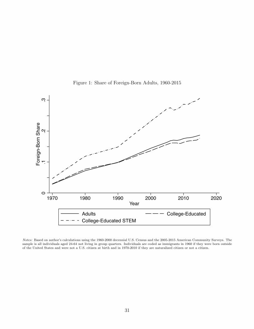
Figure 1: Share of Foreign-Born Adults, 1960-2015
0.1
.2.3
Fore
ign-
Born
Sha
re
1970 1980 1990 2000 2010 2020Year
Adults College-EducatedCollege-Educated STEM
Notes: Based on author’s calculations using the 1960-2000 decennial U.S. Census and the 2005-2015 American Community Surveys. Thesample is all individuals aged 24-64 not living in group quarters. Individuals are coded as immigrants in 1960 if they were born outsideof the United States and were not a U.S. citizen at birth and in 1970-2010 if they are naturalized citizen or not a citizen.
31

Figure 2: H-1B Immigrant Shock, 1990-2008
050
100
150
200
Num
ber o
f Pre
dict
ed Im
mig
rant
s, 1
000s
1990 1993 1996 1999 2002 2005 2008Year
0.1
.2.3
.4.5
.6H-
1B Im
mig
rant
Sho
ck
1990 1993 1996 1999 2002 2005 2008Year
All STEMBusiness HealthcareSocial Sciences Liberal ArtsEducation Other
Notes: Based on author’s calculations using the 2010-2012 American Community Survey (ACS) and the 2010-2015 Office of ForeignLabor Certification (OFLC) Disclosure Data for the H-1B Visa Program. The left panel plots the predicted number of immigrants toenter the United States each year due to the H-1B visa program. The solid line plots the program cap in October of each calendar year.The remaining remaining lines plot the number of immigrants by college major based on the distribution of occupation in the OFL andthe joint distribution of majors and occupation in the ACS. The right panel plots the size of the immigrant shock and is the numberof immigrants relative to the number of natives that entered the workforce in that year. See Table A-1 for the categorization of ACSdegrees and Table A-3 for estimated shares.
32

Figure 3: Predicting the 2010 Immigrant Shock with Changes in H-1B Policy
-.3-.2
-.10
.1.2
.3.4
.5.6
Actu
al Im
mig
rant
Sho
ck (R
esid
ual)
-.3 -.2 -.1 0 .1 .2 .3 .4H-1B Immigrant Shock (Residual)
Notes: Based on author’s calculations using the 2010-2012 American Community Survey (ACS) and the 2010-2015 Office of ForeignLabor Certification (OFLC) Disclosure Data for the H-1B Visa Program. Each point represent a major-cohort cell for 40 college majorgroupings and 19 cohorts. The figure plots the estimated H-1B immigrant shock and the actual immigrant shock for each major-cohortcell net of major and cohort fixed effects on the horizontal axis and vertical axis, respectively. All major-cohort observations are weightedby the number of native observations in the cell. The dashed line is the 45-degree line and the solid line is the fitted line from weightedleast squares regression.
33

Figure 4: The Effect of High-Skilled Immigration on Native Earnings: OLS vs. Reduced-Form
-.2-.1
0.1
.2M
ean
Log
Wee
kly
Wag
e (R
esid
ual)
-.2 0 .2 .4 .6Actual Immigrant Shock (Residual)
(a) WLS
-.2-.1
0.1
.2M
ean
Log
Wee
kly
Wag
e (R
esid
ual)
-.2 -.1 0 .1 .2 .3Predicted Immigrant Shock (Residual)
(b) IV
Notes: Based on author’s calculations using the 2010-2012 American Community Survey (ACS) and the 2010-2015 Office of ForeignLabor Certification (OFLC) Disclosure Data for the H-1B Visa Program. Each point represent a major-cohort cell for 40 college majorgroupings and 19 cohorts. The figure in the left panel plots the actual immigrant shock and average log weekly earnings for each major-cohort cell net of major and cohort fixed effects on the horizontal axis and vertical axis, respectively. The figure in the right panel plotsthe predicted immigrant shock from the first-stage IV and average log weekly wages for each major-cohort cell net of major and cohortfixed effects on the horizontal axis and vertical axis, respectively. All major-cohort observations are weighted by the number of nativeobservations in the cell. The solid line is the fitted line from weighted least squares regression.
34

Table 1: College Major Distribution by Nativity Status
Natives Immigrants Natives Immigrants Natives Immigrants(1) (2) (3) (4) (5) (6)
STEM vs. Non-STEMSTEM 17.6 35.3 26.4 49.7 9.9 21.8Non-STEM 82.4 64.7 73.6 50.3 90.1 78.2
Conditional on Non-STEMBusiness 28.2 37.1 38.4 45.8 20.8 31.8Healthcare 8.4 12.9 3.2 7.5 12.1 16.2Social Sciences 25.0 17.6 24.7 16.5 25.1 18.3Liberal Arts 8.6 9.3 8.5 8.4 8.6 9.8Education 16.2 9.9 9.1 5.9 21.4 12.3Other 13.7 13.2 16.1 15.9 12.0 11.5Notes: Based on author's calculations using the 2010-2012 American Community Survey. The sample is all college graduates, aged 24-64, and not living in group quarters. College majors are based on the first degree reported by the respondent and are classified into groups according to Appendix Table XXX.
All Men Women
Notes: Based on author’s calculations using the 2010-2012 American Community Survey. The sample is all college graduates aged 24-64that are not living in group quarters. College majors are based on the first degree reported by the respondent and are classified intoseven broad major groups according to Table A-1.
35

Table 2: Occupational Distributions by Education Group
(1)Panel A: Aggregated Top 5 Occupation SharesAll Workers 0.22Only College Educated 0.37Within-Major (Average) 0.49Panel B: Index of SimilarityCollege vs. Non-College Workers 0.45One Major vs. Other Majors (Average) 0.65Within-Major Immigrant vs. Native (Average) 0.80Notes: Based on author's calculations using the 2010-2012 American Community using 3-digit SOC codes that have been cleaned to construct a crosswalk of occupations between the ACS and H-1B program data. The sample of all workers includes all adults aged 24-64 not living in group quarters that have a valid occupation code. Workers with a bachelor's degree are grouped into one of forty college majors. Panel A displays the combined shares of the five largest occupations for all workers in the sample and only those that have completed a bachelor's degree. The share is then calculated separately for each major and averaged. Panel B reports the index of similarity. The index is calculated comparing college graduates to noncollege graduates, each college major to college graduates not in that major, amd natives and immigrants with the same college major.
Notes: Based on author’s calculations using the 2010-2012 American Community and 3-digit SOC codes that have been cleaned toconstruct a crosswalk of occupations between the ACS and H-1B program data. The sample includes all adults aged 24-64 not living ingroup quarters that have a valid occupation code. Workers with a bachelor’s degree are grouped into one of forty college majors. Panel Adisplays the combined shares of the five largest occupations in each row for all workers in the sample and only those that have completeda bachelor’s degree. The share is then calculated separately for each major and averaged. Panel B reports the index of similarity. Theindex in each row is calculated comparing college graduates to noncollege graduates, each college major to college graduates not in thatmajor, and natives and immigrants with the same college major, respectively.
36

Table 3: Predicting the 2010 Immigrant Shock with Changes in H-1B Policy
H-1B Shock(1) (2) (3) (4)
H-1B Immigrant Shock 0.669** 0.641** 0.439*(0.198) (0.192) (0.176)
Unemployment Rate -10.53** -10.02** -1.538(3.294) (3.172) (0.955)
Major fixed effects Yes Yes Yes YesCohort fixed effects Yes Yes Yes YesMajor-specific linear cohort trend No No Yes Yes
F -statistic 11.39 11.12 6.20 -Observations 760 760 760 760
Immigrant Shock
Notes: Data are from the 2010-2012 American Community Survey, the 1990-2008 monthly Current Population Survey, and 2010-2015Office of Foreign Labor Certification (OFLC) Disclosure Data for the H-1B Visa Program. The dependent variable is the major-cohortimmigrant shock calculated in the 2010-2012 ACS. All college-educated individuals are grouped into 40 college majors and 19 cohortsbased on entry into the U.S. labor market from 1990-2008. Individuals are grouped by year of birth and are assumed to enter the labormarket at age 22. Immigrants are grouped based on year of entry into the United States if they entered after age 22. Specification (1)includes major and cohort fixed effects. Specification (2) controls for the major-specific unemployment rate upon entry into the U.S.labor market. The unemployment rate is calculated by converting occupation-specific unemployment rates estimated in the monthlyCPS into major-specific rates using the IPUMS 2010 harmonized occupation codes and the major-occupation distribution estimatedin the 2010-2012 ACS. Specfication (3) adds major-specific linear cohort trends. In column (4), the dependent variable is the H-1Bimmigrant shock. Robust standard errors are in parentheses and are clustered by major. All regressions are weighted the number ofnative observations in a major-cohort cell. The reported F -statistic is from the test of the null hypothesis that the coefficient on theH-1B immigrant shock is zero.
** Significant at the 1 percent level* Significant at the 5 percent level+ Significant at the 10 percent level
37

Table 4: The Effect of High-Skilled Immigration on Native Earnings
WLS WLS WLS IV IV IV(1) (2) (3) (4) (5) (6)
Panel A: Average Log Weekly EarmingsImmigrant Shock 0.0343 0.0458 0.00937 -0.0641* -0.0646* -0.118*
(0.0403) (0.0460) (0.0347) (0.0306) (0.0329) (0.0503)Unemployment Rate 1.165 0.319 -0.123 -1.042
(1.772) (1.107) (1.723) (1.401)
Panel B: Average Log Annual EarningsImmigrant Shock 0.0379 0.0490 0.00656 -0.0656* -0.0664* -0.125*
(0.0417) (0.0471) (0.0349) (0.0312) (0.0332) (0.0526)Unemployment Rate 1.128 0.287 -0.218 -1.120
(1.856) (1.140) (1.807) (1.453)
Panel C: Average Log Hourly EarningsImmigrant Shock 0.0328 0.0472 0.0122 -0.0635* -0.0629+ -0.127*
(0.0378) (0.0447) (0.0328) (0.0306) (0.0324) (0.0637)Unemployment Rate 1.450 0.817 0.167 -0.667
(1.601) (1.166) (1.533) (1.528)
Major fixed effects Yes Yes Yes Yes Yes YesCohort fixed effects Yes Yes Yes Yes Yes YesMajor-specific linear trend No No Yes No No Yes
F -statistic - - - 11.39 11.12 6.20Observations 760 760 760 760 760 760
Notes: Data are from the 2010-2012 American Community Survey, the 1990-2008 monthly Current Population Survey, and 2010-2015 Office of Foreign Labor CertificationDisclosure Data for the H-1B Visa Program. The dependent variables are major-cohort cell averages of log earnings using weekly earnings in Panel A, annual earnings in PanelB, and hourly earnings in Panel C. All college-educated individuals are grouped into 40 college majors and 19 cohorts based on entry into the U.S. labor market from 1990-2008.Individuals are grouped by year of birth and are assumed to enter the labor market at age 22. Immigrants are grouped based on year of entry into the United States if theyarrived after the age of 22. The explanatory variable is the ratio of immigrants to natives in a major-cohort cell in the 2010-2012 ACS. Column (1)-(3) is estimated usingweighted least squares. Columns (4)-(6) are estimated using two-stage weighted least squares where the instrument is the ratio of the estimated H-1B immigrants to the numberof natives in the 2010-2012 ACS. Earnings are constructed by averaging over all natives. All regressions are weighted by the number of native observations in a major-cohortcell. Standard errors are reported in parentheses and are clustered at the major level.
** Significant at the 1 percent level* Significant at the 5 percent level+ Significant at the 10 percent level
38

Table 5: The Effect of High-Skilled Immigration on Native Earnings by Group
All Men Women White Black(1) (2) (3) (4) (5)
Panel A: Average Log Weekly EarmingsImmigrant Shock -0.118* -0.168** -0.0897 -0.114* 0.0936
(0.0503) (0.0465) (0.103) (0.0513) (0.0958)Unemployment Rate -1.042 -0.141 -1.406 -0.914 1.233
(1.401) (1.561) (2.103) (1.314) (2.495)
Panel B: Average Log Annual EarningsImmigrant Shock -0.125* -0.188** -0.0952 -0.119* 0.0833
(0.0526) (0.0508) (0.112) (0.0524) (0.0795)Unemployment Rate -1.120 -0.386 -1.629 -0.947 1.070
(1.453) (1.667) (2.123) (1.357) (2.356)
Panel C: Average Log Hourly EarningsImmigrant Shock -0.127* -0.140* -0.0452 -0.114* 0.0725
(0.0637) (0.0669) (0.0951) (0.0574) (0.106)Unemployment Rate -0.667 0.322 -0.244 -0.689 1.937
(1.528) (1.589) (1.929) (1.354) (2.382)
Major fixed effects Yes Yes Yes Yes YesCohort fixed effects Yes Yes Yes Yes YesMajor-specific linear trend Yes Yes Yes Yes Yes
F -statistic 6.20 6.20 6.20 6.20 6.20Observations 760 760 760 760 758
Notes: Data are from the 2010-2012 American Community Survey, the 1990-2008 monthly Current Population Survey, and 2010-2015 Office of Foreign Labor CertificationDisclosure Data for the H-1B Visa Program. The dependent variables are major-cohort cell averages of log earnings using weekly earnings in Panel A, annual earnings inPanel B, and hourly earnings in Panel C. All college-educated individuals are grouped into 40 college majors and 19 cohorts based on entry into the U.S. labor market from1990-2008. Individuals are grouped by year of birth and are assumed to enter the labor market at age 22. Immigrants are grouped based on year of entry into the United Statesif they arrived after the age of 22. The explanatory variable is the ratio of immigrants to natives in a major-cohort cell in the 2010-2012 ACS. All columns are estimated usingtwo-stage weighted least squares where the instrument is the ratio of the estimated H-1B immigrants to the number of natives in the 2010-2012 ACS. Eanings are constructedby averaging over all natives in the listed subgroup. All regressions are weighted by the number of native observations in a major-cohort cell. Standard errors are reported inparentheses and are clustered at the major level.
** Significant at the 1 percent level* Significant at the 5 percent level+ Significant at the 10 percent level
39

Table 6: The Effect of High-Skilled Immigration on Native Employment
WLS IV WLS IV WLS IVDependent Variable Sample: (1) (2) (3) (4) (5) (6)All Natives 0.00666 0.0785+ -0.0169 0.0228 -0.00913 0.00685(N=760) (0.0169) (0.0460) (0.0263) (0.0382) (0.0192) (0.0281)
Native Men -0.0142 0.0160 -0.0695+ -0.0931** -0.0406 -0.0778**(N=760) (0.0216) (0.0328) (0.0400) (0.0356) (0.0286) (0.0259)
Native Women -0.00385 0.0455 -0.0201 -0.0357 -0.0200 -0.0416(N=760) (0.0192) (0.0486) (0.0323) (0.0426) (0.0225) (0.0423)
White Natives 0.0188 0.0960+ -0.00474 0.0471 -0.00146 0.00950(N=760) (0.0173) (0.0528) (0.0244) (0.0439) (0.0176) (0.0281)
Black Natives -0.0248 0.0582 -0.0816+ -0.0461 -0.0632 0.0227(N=758) (0.0415) (0.0665) (0.0408) (0.0690) (0.0436) (0.0764)
Major fixed effects Yes Yes Yes Yes Yes YesCohort fixed effects Yes Yes Yes Yes Yes YesMajor-specific linear trend Yes Yes Yes Yes Yes Yes
Employed Full-Time Hours (FTE)
Notes: Data are from the 2010-2012 American Community Survey, the 1990-2008 monthly Current Population Survey, and 2010-2015 Office of Foreign Labor CertificationDisclosure Data for the H-1B Visa Program. The dependent variables are major-cohort cell averages of outcomes for the group of natives indicated at the the top of the column.All college-educated individuals are grouped into 40 college majors and 19 cohorts based on entry into the U.S. labor market from 1990-2008. Individuals are grouped by yearof birth and are assumed to enter the labor market at age 22. Immigrants are grouped based on year of entry into the United States if they arrived after the age of 22. Theexplanatory variable is the ratio of immigrants to natives in a major-cohort cell in the 2010-2012 ACS. The instrument is the ratio of the estimated H-1B immigrants to thenumber of natives in the 2010-2012 ACS. Columns (1), (3), and (5) are estimated using weighted least squares and columns (2), (4), and (6) are estimated using two-stageweighted least squares where the F-statistic from the first stage is 6.20. Regressions are weighted by the number of natives observations in a cell. Standard errors are reportedin parentheses and are clustered at the major level.
** Significant at the 1 percent level* Significant at the 5 percent level+ Significant at the 10 percent level
40

Table 7: The Effect of High-Skilled Immigration on Native Occupational Earnings
Occupation Occupation Occupation OccupationAverage Average Perc. Rank Perc. Rank
Own 1990 2010 1990 2010(1) (2) (3) (4) (5)
Panel A: Pooled Native SampleImmigrant Shock -0.118* -0.0792* -0.0884+ -0.0619* -0.0566*
(0.0503) (0.0385) (0.0488) (0.0277) (0.0275)
Panel B: Male Native SampleImmigrant Shock -0.168** -0.0760+ -0.0918 -0.0579+ -0.0585+
(0.0465) (0.0434) (0.0611) (0.0297) (0.0305)
Observations 760 760 760 760 760
Notes: Data are from the 1990 U.S. decennial census, the 2010-2012 American Community Survey, the 1990-2008 monthly CurrentPopulation Survey, and 2010-2015 Office of Foreign Labor Certification (OFLC) Disclosure Data for the H-1B Visa Program. All college-educated individuals are grouped into 40 college majors and 19 cohorts based on entry into the U.S. labor market from 1990-2008.Individuals are grouped by year of birth and are assumed to enter the labor market at age 22. Immigrants are grouped based on year ofentry into the United States if they arrived after the age of 22. The dependent variable in column (1) is the major-cohort cell averagesof weekly earnings. In the remaining columns, individuals are assigned an occupation-specific wage measure: (2) average log weeklyearnings in 1990, (3) average log weekly earnings from the 2010, (4) percentile rank of weekly earnings in 1990, and (5) percentile rankof weekly earnings in 2010. Wage measures from 1990 are assigned using the IPUMS 2010 harmonized occupation codes and from 2010using the cleaned SOC occupation code used in constructing the instrument. Panel A averages the outcomes over all natives, whereasPanel B averages the outcomes using only the sample of native men. The explanatory variable is the ratio of immigrants to nativesin a major-cohort cell in the 2010-2012 ACS. The instrument is the ratio of the estimated H-1B immigrants to the number of nativesin the 2010-2012 ACS. All specifications include major fixed effects, cohort fixed effects, and major-specific linear cohort trends, andcontrol for the major-specific unemployment rate upon entering the U.S. labor market. Regressions are weighted by the number of nativeobservations in a cell. Standard errors are reported in parentheses and are clustered at the major level.
** Significant at the 1 percent level* Significant at the 5 percent level+ Significant at the 10 percent level
41

Table 8: The Effect of High-Skilled Immigration on Native Tasks
Interactive / Interactive / Leadership /Complex Cog. Quantitative Quantitative
(Caines et al. 2016) (Peri & Sparber 2011)(1) (2) (3)
Panel A: Pooled Native SampleImmigrant Shock 0.0775** 0.0401* 0.0608*
(0.0291) (0.0170) (0.0268)
Panel B: Male Native SampleImmigrant Shock 0.0454 0.0202 0.0651*
(0.0318) (0.0286) (0.0323)
Observations 760 760 760
Notes: Data are from the 2010-2012 American Community Survey, the 1990-2008 monthly Current Population Survey, 2010-2015 Office of Foreign Labor Certification (OFLC)Disclosure Data for the H-1B Visa Program, and the O*NET 21.1 database. All college-educated individuals are grouped into 40 college majors and 19 cohorts based on entryinto the U.S. labor market from 1990-2008. Individuals are grouped by year of birth and are assumed to enter the labor market at age 22. Immigrants are grouped based on yearof entry into the United States if they arrived after the age of 22. The dependent variables are ratios of the percentile ranks of task-importance on current occupation. Column(1) compares interactive to complex cognitive tasks using classifications from Caines et al. (2016). Column (2) compares interactive to quantitative tasks using classificationsPeri and Sparber (2011). Column (3) compares leadership to quantitative activities where the latter group is drawn from Peri and Sparber (2011). Panel A uses all natives,whereas Panel B uses only the sample of native men. The explanatory variable is the ratio of immigrants to natives in a major-cohort cell in the 2010-2012 ACS. The instrumentis the ratio of the estimated H-1B immigrants to the number of natives in the 2010-2012 ACS. All specifications include major fixed effects, cohort fixed effects, major-specificlinear cohort trends, and control for the major-specific unemployment rate upon entering the U.S. labor market. Regressions are weighted by the number of native observationsin a cell. Standard errors are reported in parentheses and are clustered at the major level.
** Significant at the 1 percent level* Significant at the 5 percent level+ Significant at the 10 percent level
42

Table 9: Estimates of the Elasticity of Substitution between STEM and Non-STEM Majors
(1) (2) (3) (4)Panel A: All Wage SampleLog Relative Hours Worked -0.219* -0.210*
(0.0903) (0.0902)Log Relative Efficiency Units -0.194+ -0.186+
(0.0971) (0.0970)
Estimate of Elasticity of Substitution 4.57 4.76 5.15 5.38 between STEM and Non-STEMPanel B: Full-Time Wage SampleLog Relative Hours Worked -0.311** -0.306**
(0.0865) (0.0888)Log Relative Efficiency Units -0.276** -0.271**
(0.0950) (0.0973)
Estimate of Elasticity of Substitution 3.22 3.27 3.62 3.69 between STEM and Non-STEMWeight ACS Obs. Var. Weight ACS Obs. Var. WeightObservations 102 102 102 102
Notes: Data are from the 2010-2015 American Community Surveys. The sample is all college-educated individuals aged 24-63 not livingin group quarters. The unit of observation is a state-period cell, where the ACS is pooled across the 2010-2012 and 2013-2015 surveys.Workers are grouped into STEM and non-STEM majors. The dependent variable is the difference in average log weekly earnings betweenSTEM and non-STEM college majors. The explanatory variable is the difference in log labor supply between STEM and non-STEMcollege majors. In columns (1) and (2), total hours worked for all workers in a state-period cell are used. In columns (3) and (4), STEMand non-STEM efficiency units are calculated using an Armington aggregator over eight 5-year experience groups. Relative productivitiesare estimated by replicating Borjas (2014) and an elasticity of substitution across experience groups of 6.54 (1/0.153) is used. Thecoefficient on the explanatory variable represents the inverse of the elasticity of substitution between STEM and non-STEM and isreported below the results. Panel A constructs wages using the wage sample and Panel B uses full-time workers only. All specificationsinclude state fixed effects and period fixed effects. Regressions are weighted by the number of observations in a cell (columns (1) and(3)) and inverse variance weight (columns (2) and (4)). Robust standard errors are reported in parentheses.
** Significant at the 1 percent level* Significant at the 5 percent level+ Significant at the 10 percent level
43

Table 10: Simulated Increase in Non-STEM Wages Relative to STEM Wages Due to Immigration,1990-2010
College Major STEM OccupationShock Shock
(1) (2)Lower Bound: ! = 2 12.1% 7.3%FT Wage Estimate: ! = 3.5 6.9% 4.2%All Wage Estimate: ! = 5 4.8% 2.9%Upper Bound: ! = 6.7 3.6% 2.2%
Notes: Based on author’s calculations using the 1990 U.S. decennial census and the 2010-2012 American Community Survey. Incomeshares are calculated using the 2010-2012 ACS. The immigrant shock in column (1) is calculated based on an individual’s college major.An individual’s college major in 1990 is imputed based on their IPUMS 2010 harmonized occupation code. The immigrant shock incolumn (2) is calculated based on an individual’s IPUMS 1990 harmonized occupation code. Each row represents a different wagesimulation based on difference values of the elasticity of substitution between STEM and non-STEM workers. Each value represents thesimulated increase in non-STEM wages relative to STEM wages due to the immigrant shock experienced between 1990 and 2010. Seetext for specifics on relative wage calculations.
44

A Appendix
45

Table A-1: College Major Classification
Skill Group College Major IPUMS Detailed CodeSTEM Computer Science 2100, 2101, 2102, 2105, 2106, 2107
Math 3700, 3701, 3702, 4005Engineering 2400, 2401, 2402, 2403, 2404, 2405, 2406, 2407, 2408, 2409,
2410, 2411, 2412, 2413, 2414, 2415, 2416, 2417, 2418, 2419, 2499, 2500, 2501, 2502, 2503, 2504, 2599, 3801, 5008
Life Sciences 1103, 1104, 1105, 1106, 1301, 3600, 3601, 3602, 3603, 3604, 3605, 3606, 3607, 3608, 3609, 3611, 3699, 4006
Physical Sciences 5000, 5001, 5002, 5003, 5004, 5005, 5006, 5007Business Accounting 6201
Economics 1102, 5501Finance 6202, 6207Marketing 6206Business Management 6203Other Business 6200, 6204, 6205, 6209, 6210, 6211, 6212, 6299
Healthcare Pharmacy & Medical Prep 6106, 6108Nursing 6107Technical Health Fields 4002, 5102, 6100, 6102, 6103, 6104, 6105, 6109, 6199
Social Sciences Communication 1901, 1902, 1903, 1904, 2001Political Science, International Relations, Pre- Law & Legal Studies
3201, 3202, 5505, 5506
Sociology 5507History 6402, 6403Pschology 5200, 5201, 5202, 5203, 5205, 5206, 5299Public Admin, Public Policy, and Public Helath 5401, 5402, 6110Social Work 5403, 5404Social Science Fields, Other 1501, 4001, 4007, 5500, 5502, 5503, 5504, 5599
Liberal Arts Philosophy 4801, 4901Liberal Arts and Humanities 3401, 3402Languages 2601, 2602, 2603Literature 3301, 3302
Education Early and Elementary Education 2304, 2307Secondary Education 2309General Education 2300, 2312Field Specific Education 2305, 2306, 2308, 2311, 2313, 2314Special Needs Education 2310Other Education 2301, 2303, 2399, 3501
Other Agriculture, Forestry, and Natural Resources 1100, 1101, 1199, 1302, 1303Architecture 1401Family and Consumer Sciences 2901Visual and Performing Arts 6000, 6001, 6002, 6003, 6005, 6006, 6007, 6099Leisure Studies 4101Industrial and Commercial Arts 6004Protective Services 5301Other Fields 2201, 4000, 5098, 5601, 5701, 5901
Notes: College Majors are grouped into 7 broad classifications: STEM, Business, Healthcare, Social Sciences, Liberal Arts, Education,and Other. The forty detailed major groups are listed in the second column. The corresponding codes for the IPUMS ACS variabledegfieldd are given in the third column.
46

Table A-2: Three Largest H-1B Occupations
(1)Panel A: Computer and Information Research Scientist (15-1121)Share of all H-1B Applications, 2010-2015 17.9%Share of Occupation in College Major, 2010-2012
Computer science 21.4%Engineering 16.0%Other business 10.1%Business management 7.8%Finance 4.5%All other majors 40.2%
Panel B: Software Developers, Applications, and Systems Software (15-113X)Share of all H-1B Applications, 2010-2015 17.1%Share of Occupation in College Major, 2010-2012
Computer science 35.0%Engineering 33.6%Math 4.5%Other business 4.4%Physical sciences 3.3%All other majors 19.1%
Panel C: Computer Programmers (15-1131)Share of all H-1B Applications, 2010-2015 13.9%Share of Occupation in College Major, 2010-2012
Computer science 41.7%Engineering 18.1%Other business 6.2%Math 6.0%Business Management 4.0%All other majors 24.0%
Notes: Based on author’s calculations using the 2010-2012 American Community Survey and 2010-2015 Office of Foreign Labor Cer-tification Disclosure Data for the H-1B Visa Program. To compare occupations across datasets, I first construct a crosswalk betweenthe SOC codes found in the H-1B data and the ACS file. Each panel represents a different occupation. The share of the occupation inthe H-1B data is calculated all applications from 2010-2015. The occupation-specific college major distributions are calculated using allworkers aged 24-55 with a bachelor’s degree or higher that are not living in group quarters and have a nonmissing occupation code.
47

Table A-3: Estimated Share of H-1B Visas, by College Major
Panel A: Broad Major GroupsSTEM 54.18 Liberal Arts 3.63Business 20.51 Healthcare 2.90Social Sciences 10.17 Education 2.39Other 6.29
Panel B: All College MajorsEngineering* 21.03 Industrial and Commercial Arts 0.81Computer Sci.* 20.17 General Educ 0.75Other Business 6.39 Field Specific Educ 0.67Life Sciences* 5.96 Liberal Arts and Humanities 0.67Business Mgmt. 5.13 Sociology 0.66Physical Sciences* 3.51 Languages 0.64Math* 3.51 Philosophy 0.64Accounting 2.87 Nursing 0.61Communication 2.69 Protective Services 0.58Finance 2.37 Architecture 0.58Pschology 2.34 Agriculture/Forestry/Natural Resources 0.56Economics 2.19 Pharmacy / Medical Prep 0.55Technical Health Fields 1.74 Early and Elem. Educ 0.54Poli. Sci./Intl Relations/Pre-Law/Legal Studies 1.70 Leisure Studies 0.42Literature 1.68 Public Admin/Policy/Helath 0.26Visual and Performing Arts 1.66 Social Work 0.24Marketing 1.55 Family and Consumer Sciences 0.24Other Fields 1.44 Other Educ 0.17Social Science Fields, Other 1.20 Special Needs Educ 0.14History 1.08 Secondary Educ 0.12
Notes: Based on author’s calculations using the 2010-2012 American Community Survey and 2010-2015 Office of Foreign Labor Certification Disclosure Data for the H-1B VisaProgram. See text for additional details on the data and the process to assign LCA data at the occupation level to specific college majors. Panel A provides estimated shares forthe 7 broad college major groups from Table A-1. Panel B provides the shares used in analysis to construct the immigrant instrument for each of forty college majors. STEMmajors are denoted by an asterisk.
48

Table A-4: Leadership Aggregate Classification - O*NET 21.1
Detailed O*NET Activity O*NET ElementCoordinating the Work and Activity of Others 4.A.4.b.1Developing and Building Teams 4.A.4.b.2Training and Teaching Others 4.A.4.b.3Guiding Directing and Motivating Subordinates 4.A.4.b.4Coaching and Developing Others 4.A.4.b.5Staffing Organizational Units 4.A.4.c.2
Notes: O*NET Activities are categorized into related groups. In this paper, I group six activities listed in the table into a Leadershipindex. The paper also uses other classifications. See the text of Caines et al. (2016) and Peri and Sparber (2011) for details.
49

Table A-5: The Effect of High-Skilled Immigrant on Native Weekly Earnings, Robustness Checks
WLS IV WLS IV WLS IV WLS IV(1) (2) (3) (4) (5) (6) (7) (8)
Immigrant shock 0.00937 -0.118* 0.0253 -0.0800*(0.0347) (0.0503) (0.0327) (0.0347)
Immigrant shock (under 40) 0.0149 -0.131*(0.0367) (0.0557)
Immigrant Share 0.0297 -0.231(0.0780) (0.212)
Unemployment rate 0.319 -1.042 0.372 -1.131 0.333 -0.670 -0.699 -1.825+(1.107) (1.401) (1.105) (1.441) (1.011) (1.494) (1.213) (1.069)
Major fixed effects Yes Yes Yes Yes Yes Yes Yes YesCohort fixed effects Yes Yes Yes Yes Yes Yes Yes YesMajor-specific linear trend Yes Yes Yes Yes Yes Yes Yes Yes
F -statistic - 6.20 - 7.60 - 44.29 - 6.20Observations 760 760 760 760 760 760 760 760
Median EarningsAverage Earnings
Notes: Data are from the 2010-2012 American Community Survey, the 1990-2008 monthly Current Population Survey, and 2010-2015 Office of Foreign Labor CertificationDisclosure Data for the H-1B Visa Program. The dependent variable is major-cohort cell averages of log weekly earnings for columns (1)-(6) and the median log weekly earningsfor columns (7)-(8). All college-educated individuals are grouped into 40 college majors and 19 cohorts based on entry into the U.S. labor market from 1990-2008. Individualsare grouped by year of birth and are assumed to enter the labor market at age 22. Immigrants are grouped based on year of entry into the United States if they arrived afterthe age of 22. In columns (1)-(2), the explanatory variable is the ratio of immigrants to natives in a major-cohort cell in the 2010-2012 ACS. In columns (3)-(4), immigrantswho entered the U.S. after age 40 are removed from the explanatory variable. In columns (5)-(6), the explanatory variable is the share of immigrants in the major-cohort cell.All specifications control for college major and cohort fixed effects, the major-specific unemployment rate at labor market entry, and major-specifc linear cohort trends. Allregressions are weighted by the number of native observations in a major-cohort cell. Standard errors are reported in parentheses and are clustered at the major level.
** Significant at the 1 percent level* Significant at the 5 percent level+ Significant at the 10 percent level
50

Table A-6: The Effect of High-Skilled Immigrant on Native Weekly Earnings, Alternative Weights
Pooled Men Pooled MenWeights used: (1) (2) (3) (4)Unweighted -0.0632 -0.153* -0.0282 -0.108
(0.0618) (0.0661) (0.0662) (0.0663)Number of native observations in major-cohort cell -0.118* -0.168** -0.0871+ -0.133**
(0.0503) (0.0465) (0.0488) (0.0492)Number of native observations used to average wages -0.119* -0.195** -0.0975* -0.157**
(0.0503) (0.0413) (0.0467) (0.0426)Sample variance of average wages -0.115* -0.200** -0.0969* -0.166**
(0.0483) (0.0429) (0.0433) (0.0444)
All Workers Full-Time Workers
Notes: Data are from the 2010-2012 American Community Survey, the 1990-2008 monthly Current Population Survey, and 2010-2015 Office of Foreign Labor Certification(OFLC) Disclosure Data for the H-1B Visa Program. The dependent variables are major-cohort cell averages of log earnings using weekly earnings. All college-educatedindividuals are grouped into 40 college majors and 19 cohorts based on entry into the U.S. labor market from 1990-2008. Individuals are grouped by year of birth and areassumed to enter the labor market at age 22. Immigrants are grouped based on year of entry into the United States if they arrived after the age of 22. The explanatory variableis the ratio of immigrants to natives in a major-cohort cell in the 2010-2012 ACS which is instrumented by the ratio of the estimated H-1B immigrants to the number of nativesin the 2010-2012 ACS. Earnings in columns (1) and (3) are constructed by averaging over all natives and in columns (2) and (4) by averaging over the earnings of males. Eachrow is weighted by the weight listed in the left column. Standard errors are reported in parentheses and are clustered at the major level.
** Significant at the 1 percent level* Significant at the 5 percent level+ Significant at the 10 percent level
51

Table A-7: The Effect of High-Skilled Immigrant on Native Tasks
Beta Std. Error Beta Std. ErrorTask: (1) (2) (3) (4)Analytical or Quantitative TasksAnalyze Data or Information -0.0506* (0.0246) -0.0523 (0.0341)Deductive Reasoning -0.0532* (0.0236) -0.0520 (0.0316)Inductive Reasoning -0.0558+ (0.0288) -0.0541 (0.0391)Estimating Quantifiable Characteristics 0.0221 (0.0301) 0.0432 (0.0290)Mathematical Reasoning -0.0160 (0.0205) -0.0221 (0.0220)
Interactive or Communication TasksResolving Conflicts / Negotiating 0.0208 (0.0263) 0.00299 (0.0213)Communicating Within Organization 0.0196 (0.0277) 0.0318 (0.0324)Communicating Outside Organization 0.00387 (0.0229) -0.00458 (0.0288)Oral Comprehension -0.0334+ (0.0174) -0.0325 (0.0259)Written Comprehension -0.0253 (0.0180) -0.0288 (0.0253)Written Expression -0.0576** (0.0220) -0.0579+ (0.0306)Oral Expression -0.0584** (0.0214) -0.0635* (0.0293)
Leadership / Management:Coordinate Others' Work Activities -0.00544 (0.0252) -0.00403 (0.0305)Develop and Build Teams 0.00563 (0.0280) 0.0183 (0.0335)Training and Teaching Others -0.0318+ (0.0177) -0.0141 (0.0267)Guide, Direct, and Motivate Subordinates 0.0124 (0.0336) 0.0285 (0.0381)Coach and Develop Others -0.0185 (0.0221) -0.00744 (0.0272)Staff Organizational Units 0.0498 (0.0479) 0.0435 (0.0461)
Pooled Natives Male Natives
Notes: Data are from the 2010-2012 American Community Survey, the 1990-2008 monthly Current Population Survey, 2010-2015 Officeof Foreign Labor Certification (OFLC) Disclosure Data for the H-1B Visa Program, and the O*NET 21.1 database. All college-educatedindividuals are grouped into 40 college majors and 19 cohorts based on entry into the U.S. labor market from 1990-2008. Individualsare grouped by year of birth and are assumed to enter the labor market at age 22. Immigrants are grouped based on year of entry intothe United States if they arrived after the age of 22. The dependent variables are percentile ranks of the importance of groups of tasksbased on current occupation. Tasks are grouped by their correspondence to the Peri and Sparber (2011) index. The last group are tasksrelated to leadership or management. Column 1 averages the outcomes over all natives, whereas column 3 averages the outcomes usingonly the sample of native men. The explanatory variable is the ratio of immigrants to natives in a major-cohort cell in the 2010-2012ACS. The instrument is the ratio of the estimated H-1B immigrants to the number of natives in the 2010-2012 ACS. All specificationsinclude major fixed effects, cohort fixed effects, and major-specific linear cohort trends, and control for the major-specific unemploymentrate upon entering the U.S. labor market. Regressions are weighted by the number of native observations in a cell. Standard errors arereported in parentheses and are clustered at the major level.
** Significant at the 1 percent level* Significant at the 5 percent level+ Significant at the 10 percent level
52