Prep

rint

Noname manuscript No.(will be inserted by the editor)

C. J. Pipe · T. S. Majmudar · G. H. McKinley

High Shear Rate Viscometry

the date of receipt and acceptance should be inserted later

Abstract We investigate the use of two distinct and complementary approaches to measuring the vis-

cometric properties of low viscosity complex fluids at high shear rates up to 80,000 s−1. Firstly we adapt

commercial controlled-stress and controlled-rate rheometers to access elevated shear rates by using par-

allel plate fixtures with very small gap settings (down to 30 µm). The resulting apparent viscosities are

gap-dependent and systematically in error but the data can be corrected - at least for Newtonian fluids -

via a simple linear gap correction originally presented by Connelly & Greener (1985). Secondly we use a

microfabricated rheometer-on-a-chip to measure the steady flow curve in rectangular microchannels. The

Weissenberg-Rabinowitsch-Mooney analysis is used to convert measurements of the pressure-drop/flow-

rate relationship into the true wall-shear rate and the corresponding shear-rate-dependent viscosity. Mi-

crochannel measurements are presented for a range of Newtonian calibration oils, a weakly shear-thinning

dilute solution of poly(ethylene oxide), a strongly shear-thinning, concentrated solution of xanthan gum

and a wormlike micelle solution that exhibits shear-banding at a critical stress. Excellent agreement

between the two approaches is obtained for the Newtonian calibration oils, and the relative benefits

of each technique are compared and contrasted by considering the physical processes and instrumental

limitations that bound the operating spaces for each device.

Hatsopoulos Microfluids Laboratory, Department of Mechanical Engineering, Massachusetts Institute of Technol-

ogy, Cambridge, MA 02139, USA

Prep

rint

1 Introduction

The behaviour of complex liquids at large deformation rates is relevant in many processes involving

coating, spraying, lubrication and injection molding. Although both shear and extensional deformations

can be important in complex flows, in this study we concentrate on the rheological behaviour in steady

shearing flow. From dimensional analysis we expect γ ∼ U/L, where U is a characteristic velocity

difference acting over a characteristic distance L, indicating that to attain high shear rates it is necessary

to either (a) increase U or (b) decrease L. Large velocities can lead to high Reynolds numbers Re =

ρUL/η, where ρ is the density and η the dynamic viscosity of the fluid, and loss of viscometric flow. Thus

it is usual to strive to minimize L and the limiting factor in accessing high shear rates is the accuracy

with which flow devices or rheological test fixtures can be manufactured and aligned so that geometric

perturbations remain small (δL/L < 1), even when L is reduced.

Various experimental configurations have been proposed for measuring viscosity at high-shear rates

including cylindrical Couette flow with narrow gaps (Merrill, 1954), torsional flow between rotating

parallel plates (Connelly & Greener, 1985; Kramer et al., 1987; Dontula et al., 1999), flow through

capillaries (Talbot, 1974; Duda et al., 1988) and slits (Laun, 1983; Lodge & de Vargas, 1983; Erickson

et al., 2002) and impact flow between a rotating ball and plate (O’Neill & Stachowiak, 1996).

Measurements using narrow gap Couette flows between concentric cylinders and between parallel-

plate fixtures have been used to measure the viscosity of Newtonian and shear-thinning liquids up to

γ ∼ 106 s−1 (Merrill, 1954; Kulicke & Porter, 1981; Connelly & Greener, 1985; Dontula et al., 1999;

Mriziq et al., 2004; Davies & Stokes, 2005) using gaps 0.5 µm ≤ H ≤ 50 µm. Suggestions that Newtonian

fluids might show a decrease in viscosity at shear rates γ ≈ 5 × 104 s−1 presented by Ram (1961) have

been re-examined by Dontula et al. (1999), who argue that the fall in viscosity of a glycerin-water

solution at high shear rates may well be due to non-viscometric flow phenomena such as viscous heating

or hydrodynamic instabilities, rather than arising from a true rate-depepndent material property.

Flows through capillaries and slit channels have also been widely used to study rheology at high shear

rates (Talbot, 1974; Laun, 1983; Lodge & de Vargas, 1983; Duda et al., 1988; Erickson et al., 2002; Kang

et al., 2005) and capillary viscometry can be an extremely simple and reliable technique for measuring

shear viscosities. However, to minimize the importance of non-viscometric flow at the entrance and exit

of the capillary it is usual to use long capillaries which can lead to long residence times for fluid elements

2

Prep

rint

in the shearing flow. Furthermore at high shear rates, an evolving thermal boundary layer resulting from

viscous heating must be accounted for (Duda et al., 1988).

Beyond the realm of classical rheometry, custom micro-fabricated devices have also been used to

measure the rheological response of complex fluids on length scales of 1–10 µm (Dhinojwala & Granick,

1997; Mukhopadhyay & Granick, 2001; Clasen & McKinley, 2004). With advances in micro- and nano-

fabrication techniques (Xia & Whitesides, 1998; Marrian & Tennant, 2003) enabling the routine and

reliable manufacture of flow devices with geometric features < 100 µm, there has been a significant

increase in studies exploiting microfluidic flow geometries for rheological characterization (Hudson et al.,

2004; Degré et al., 2006; Guillot et al., 2006; Zimmerman et al., 2006), although none of these studies

have addressed the response at high shear rates.

As the characteristic length scale of the geometry is decreased to O(1 µm), it becomes increasingly

important to separate the bulk rheological response of a sample from effects due to the confining surfaces

(McKenna, 2006). The issue of wall slip has been shown to be significant as very small length scales are

probed but nearly all experimental evidence suggests that slip, if present, occurs over length scales 0–

50 nm (Granick et al., 2003; Lauga et al., 2007) and is therefore usually negligible for most homogeneous

fluids on the micron scale. However, apparent wall slip, caused by depletion or adhesion layers at the

walls, can be detected when testing heterogeneous liquids that have distinct microstructural elements

even in flows with length scales ∼ 10 µm (Degré et al., 2006; Clasen et al., 2006).

Studies of strongly inertial flows through channels with characteristic depths O(100 µm) are reviewed

by Obot (2002) who finds that, despite some reports that the transition to turbulent flow in smooth-

walled microchannels can occur at Reynolds numbers as low as Re ≈ 200 (eg. Peng et al., 1994), the

experimental evidence so far does not support a significant decrease below the usual value for macroscale

flows Re ≤ 2000.

In the present study we compare and contrast the efficacy of two devices, a conventional rotational

parallel plate rheometer using sample gaps in the range 10 µm−500 µm, and two microfluidic slit channels

with depths of 24.6 and 50.7 µm, in order to characterize shear-dependent viscosities at deformation

rates up to 105 s−1. We show that the viscometric response at high rates for fluids ranging from constant

viscosity mineral oils to strongly shear-thinning polymer solutions and shear-banding micellar solutions

can all be determined using these techniques. We compare the results from each device to illustrate the

experimental difficulties that can be encountered in each geometry and the level of reproducibility that

3

Prep

rint

can be obtained. In Section 2 we present an overview of the fluids used in this work (2.1) as well as the

relevant analytical framework for the parallel plates geometry (2.2) and the microfluidic channels (2.3).

In Section 3.1 we investigate the use of conventional rotational rheometers to access high deformation

rates, and identify errors in zeroing the gap as a primary source of discrepancy between measured values

of apparent viscosity and the true viscosity. Using Newtonian calibration oils, we then implement a

calibration procedure originally presented by Connelly & Greener (1985) to evaluate the gap errors. We

use the resulting gap corrections to obtain true shear rates and true viscosities from the apparent values

provided by the rheometer software. In addition, we investigate two additional phenomena that can

affect the viscous response at high shear rates; centrifugal stresses, and viscous heating. In Section 3.2

we proceed to investigate the viscometric response of Newtonian fluids using micro-fluidic slit channels

equipped with flush mounted pressure sensors. We then investigate the response in both types of device

due to highly shear-thinning liquids in Section 3.3. Finally, in Section 4, we compare and contrast

the results from each device to illustrate the principal experimental difficulties associated with each

geometry and the level of reproducibility that can be obtained. The material and instrumental parameters

constraining the application of each device are then combined to produce operating space diagrams that

can guide the effective use of each approach.

2 Experimental techniques

2.1 Test fluids

Liquids exhibiting a range of viscometric behaviours, from Newtonian to strongly shear-thinning, were

investigated experimentally. Mineral oils S60 and N1000 supplied by Cannon Instrument Company (PA,

USA) and marketed as constant viscosity calibration fluids for viscometers as well as a Silicone oil (DMS

T25) from Gelest Inc. (PA, USA), were used to test the response of Newtonian fluids with nominally

constant viscosity. Henceforth, these fluids will be referred to by the labels N1, N3 and N2, respectively,

as indicated in Table 1. We also study a weakly shear-thinning solution of 0.1% poly(ethylene oxide)

(PEO) in a mixture of 55% glycerol - 44.9% distilled water (supplied by Sigma Aldrich MO, USA). The

PEO was polydisperse with viscosity – averaged molecular weight Mv = 2× 106 g/mol and the solution

was prepared with gentle mixing and rolling to avoid degradation of the polymer. The aqueous PEO

solution was then gently mixed with the glycerol for 5 minutes and left to stand for a further 24 hours.

4

Prep

rint

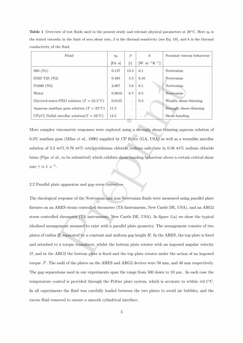
Table 1 Overview of test fluids used in the present study and relevant physical parameters at 20C. Here η0 is

the stated viscosity in the limit of zero shear rate, β is the thermal sensitivity (see Eq. 19), and k is the thermal

conductivity of the fluid.

Fluid η0 β k Nominal viscous behaviour

[Pa s] [-] [W m−1K−1]

S60 (N1) 0.137 13.5 0.1 Newtonian

DMS T25 (N2) 0.485 5.5 0.16 Newtonian

N1000 (N3) 2.867 5.6 0.1 Newtonian

Water 0.0010 6.7 0.5 Newtonian

Glycerol-water-PEO solution (T = 22.5C) 0.0155 . 0.4 Weakly shear-thinning

Aqueous xanthan gum solution (T = 22C) 11.5 . . Strongly shear-thinning

CPyCl/NaSal micellar solution(T = 22C) 14.5 . . Shear-banding

More complex viscometric responses were explored using a strongly shear-thinning aqueous solution of

0.3% xanthan gum (Milas et al., 1990) supplied by CP Kelco (GA, USA) as well as a wormlike micellar

solution of 3.2 wt%/0.76 wt% cetylpyridinium chloride/sodium salicylate in 0.56 wt% sodium chloride

brine (Pipe et al., to be submitted) which exhibits shear-banding behaviour above a certain critical shear

rate γ ≈ 1 s−1.

2.2 Parallel plate apparatus and gap error correction

The rheological response of the Newtonian and non-Newtonian fluids were measured using parallel plate

fixtures on an ARES strain controlled rheometer (TA Instruments, New Castle DE, USA), and an ARG2

stress controlled rheometer (TA instruments, New Castle DE, USA). In figure 1(a) we show the typical

idealized arrangement assumed to exist with a parallel plate geometry. The arrangement consists of two

plates of radius R, separated by a constant and uniform gap height H. In the ARES, the top plate is fixed

and attached to a torque transducer, whilst the bottom plate rotates with an imposed angular velocity

Ω, and in the ARG2 the bottom plate is fixed and the top plate rotates under the action of an imposed

torque T . The radii of the plates on the ARES and ARG2 devices were 50 mm, and 40 mm respectively.

The gap separations used in our experiments span the range from 500 down to 10 µm . In each case the

temperature control is provided through the Peltier plate system, which is accurate to within ±0.1C.

In all experiments the fluid was carefully loaded between the two plates to avoid air bubbles, and the

excess fluid removed to ensure a smooth cylindrical interface.

5

Prep

rint

In order to accurately measure the true viscosity in rotational rheometers at narrow gaps and high

shear rates, precise alignment of the parallel plates is crucial (Connelly & Greener, 1985; Kramer et al.,

1987). At very small gaps (H ≤ 10 µm), even the viscosity of air in the narrow gap between the plates

while zeroing the gap has been noted as a possible source of error (Davies & Stokes, 2005). Here we use a

calibration procedure based on the work of Connelly and Greener (Connelly & Greener, 1985) to estimate

the total effective error associated with ‘zeroing the gap’. Figure 1b shows the principal source of error in

the alignment of plates associated with axial ‘run – out’ of the shaft and the resulting non – orthogonality

between the plate and rotation axis. In a modern rotational rheometer using ‘auto-gap zeroing’ based

on electrical conductivity or friction detection, the gap is considered to be ‘zeroed’ when any point of

the top plate touches the bottom plate. A parallax in the alignment of the plates can cause the situation

shown in Figure 1b, in which the gap is considered to be zero, but in reality different parts of the upper

fixture are at different distances from the bottom plate. The maximum distance between the top fixture

and the bottom plate sets a scale for the error incurred in zeroing the gap. This error is denoted the

‘gap error’ (ε). For large gap separations (H >> ε), this error is expected to be negligible but it is of

increasing importance for small gaps. The final configuration with fluid filled between the plates is shown

in Figure 1c, where the the gap is small enough (H ∼ ε) that the effect of plate misalignment is noticeable

in the fluid sample confined within the plates. The analogous problem has been considered analytically for

the cone-and-plate rheometer by Dudgeon & Wedgewood cite[] using a domain perturbation approach.

Because the measured rheological quantities of interest such as shear rate and viscosity are dependent

on the gap height, the gap error introduces a systematic error in measured quantities in addition to the

intrinsic instrument accuracy.

Torque, displacement, and normal force are the fundamental quantities measured by the rheometer.

These raw measurements are then used to calculate stress, strain, shear rate, viscosity, and normal stress

difference. To eliminate the systematic discrepancies associated with the gap error ε and obtain accurate

values of the calculated quantities from the measured variables, it is necessary to determine the error in

gap heights via calibration, and the apparent values of measured quantities then have to be corrected

for this gap error.

There are several published procedures for assessing the gap error for parallel plate geometry (Con-

nelly & Greener, 1985; Kramer et al., 1987). We follow this method with a slightly modified analysis,

which is presented below. The procedure consists of single point tests of a Newtonian fluid of known

6

Prep

rint

viscosity under steady simple shear flow at different gaps. In the steady shear single point test on a

strain controlled rheometer, for example, a shear rate and the duration for which the specified shear rate

is to be applied is specified by the user, and the viscosity is measured after the specified equilibration

time. We have used shear rates from 10 s−1 to 100 s−1 for different fluids. The specific shear rates used

were chosen such that the measured torque was well above the minimum measurable torque. At the

beginning of the experiment the gap is zeroed to obtain a reference datum for all subsequent measured

gap heights. The fluid is then loaded and the upper plate is lowered to a specified gap height H, and

left undisturbed for 120 s to equilibrate at the specified temperature. An ‘apparent shear rate’ γa, and

the duration of measurement is then specified in the rheometer software. The duration for which the

shear rate is applied was 30 s. At the end of one single point measurement, an ‘apparent viscosity’ ηa

is reported by the software. The fluid is then removed, a new sample is loaded, and the procedure is

repeated at a different gap height H. The range of specified gap heights was decreased steadily from

500µm to 10µm.

For a given plate of radius R, specified gap height H, and angular velocity Ω, the apparent shear

rate γa at the rim of the rotating parallel plate fixture is given by:

γa =Ω R

H. (1)

The apparent viscosity ηa reported by the software is computed from the definition:

ηa =< τ >

γa, (2)

where < τ > is the expected shear stress at the rim calculated from the measured torque, T , assuming

an ideal torsional shear flow, and is given by:

< τ >≡ 2 T

π R3= ηtrue γtrue, (3)

where γtrue and ηtrue are the true shear rate at the rim and the true viscosity, respectively. Combining

Eqs. 1,2, and 3, we have,

ηa =ηtrue γtrue

ΩR/H. (4)

As discussed previously, in practice, there is always some error in zeroing the gap between the plates. For

errors of the form sketched in figure 1, the gap is always biased towards larger values than the commanded

7

Prep

rint

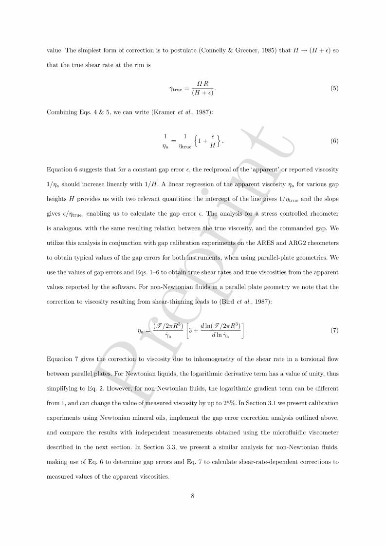
value. The simplest form of correction is to postulate (Connelly & Greener, 1985) that H → (H + ε) so

that the true shear rate at the rim is

γtrue =ΩR

(H + ε). (5)

Combining Eqs. 4 & 5, we can write (Kramer et al., 1987):

1ηa

=1

ηtrue

1 +

ε

H

. (6)

Equation 6 suggests that for a constant gap error ε, the reciprocal of the ‘apparent’ or reported viscosity

1/ηa should increase linearly with 1/H. A linear regression of the apparent viscosity ηa for various gap

heights H provides us with two relevant quantities: the intercept of the line gives 1/ηtrue and the slope

gives ε/ηtrue, enabling us to calculate the gap error ε. The analysis for a stress controlled rheometer

is analogous, with the same resulting relation between the true viscosity, and the commanded gap. We

utilize this analysis in conjunction with gap calibration experiments on the ARES and ARG2 rheometers

to obtain typical values of the gap errors for both instruments, when using parallel-plate geometries. We

use the values of gap errors and Eqs. 1–6 to obtain true shear rates and true viscosities from the apparent

values reported by the software. For non-Newtonian fluids in a parallel plate geometry we note that the

correction to viscosity resulting from shear-thinning leads to (Bird et al., 1987):

ηa =(T /2πR3)

γa

[3 +

d ln(T /2πR3)d ln γa

]. (7)

Equation 7 gives the correction to viscosity due to inhomogeneity of the shear rate in a torsional flow

between parallel plates. For Newtonian liquids, the logarithmic derivative term has a value of unity, thus

simplifying to Eq. 2. However, for non-Newtonian fluids, the logarithmic gradient term can be different

from 1, and can change the value of measured viscosity by up to 25%. In Section 3.1 we present calibration

experiments using Newtonian mineral oils, implement the gap error correction analysis outlined above,

and compare the results with independent measurements obtained using the microfluidic viscometer

described in the next section. In Section 3.3, we present a similar analysis for non-Newtonian fluids,

making use of Eq. 6 to determine gap errors and Eq. 7 to calculate shear-rate-dependent corrections to

measured values of the apparent viscosities.

8

Prep

rint

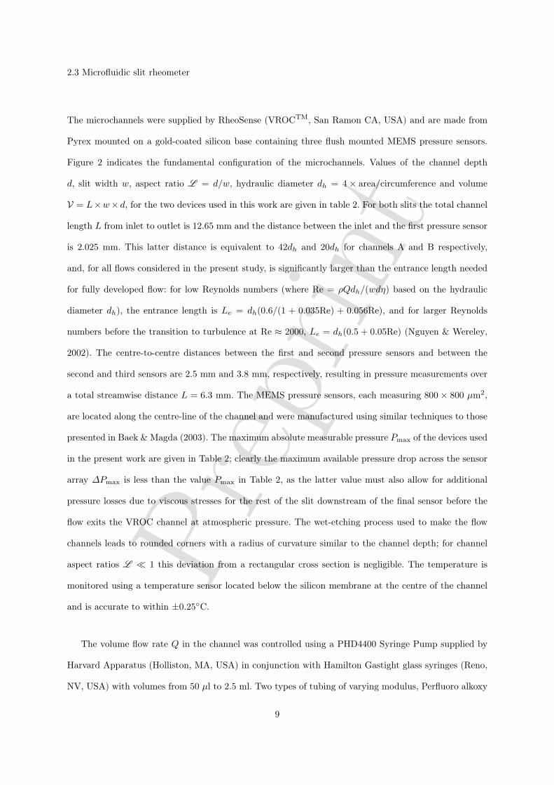
2.3 Microfluidic slit rheometer

The microchannels were supplied by RheoSense (VROCTM, San Ramon CA, USA) and are made from

Pyrex mounted on a gold-coated silicon base containing three flush mounted MEMS pressure sensors.

Figure 2 indicates the fundamental configuration of the microchannels. Values of the channel depth

d, slit width w, aspect ratio L = d/w, hydraulic diameter dh = 4× area/circumference and volume

V = L×w×d, for the two devices used in this work are given in table 2. For both slits the total channel

length L from inlet to outlet is 12.65 mm and the distance between the inlet and the first pressure sensor

is 2.025 mm. This latter distance is equivalent to 42dh and 20dh for channels A and B respectively,

and, for all flows considered in the present study, is significantly larger than the entrance length needed

for fully developed flow: for low Reynolds numbers (where Re = ρQdh/(wdη) based on the hydraulic

diameter dh), the entrance length is Le = dh(0.6/(1 + 0.035Re) + 0.056Re), and for larger Reynolds

numbers before the transition to turbulence at Re ≈ 2000, Le = dh(0.5 + 0.05Re) (Nguyen & Wereley,

2002). The centre-to-centre distances between the first and second pressure sensors and between the

second and third sensors are 2.5 mm and 3.8 mm, respectively, resulting in pressure measurements over

a total streamwise distance L = 6.3 mm. The MEMS pressure sensors, each measuring 800 × 800 µm2,

are located along the centre-line of the channel and were manufactured using similar techniques to those

presented in Baek & Magda (2003). The maximum absolute measurable pressure Pmax of the devices used

in the present work are given in Table 2; clearly the maximum available pressure drop across the sensor

array ∆Pmax is less than the value Pmax in Table 2, as the latter value must also allow for additional

pressure losses due to viscous stresses for the rest of the slit downstream of the final sensor before the

flow exits the VROC channel at atmospheric pressure. The wet-etching process used to make the flow

channels leads to rounded corners with a radius of curvature similar to the channel depth; for channel

aspect ratios L 1 this deviation from a rectangular cross section is negligible. The temperature is

monitored using a temperature sensor located below the silicon membrane at the centre of the channel

and is accurate to within ±0.25C.

The volume flow rate Q in the channel was controlled using a PHD4400 Syringe Pump supplied by

Harvard Apparatus (Holliston, MA, USA) in conjunction with Hamilton Gastight glass syringes (Reno,

NV, USA) with volumes from 50 µl to 2.5 ml. Two types of tubing of varying modulus, Perfluoro alkoxy

9

Prep

rint

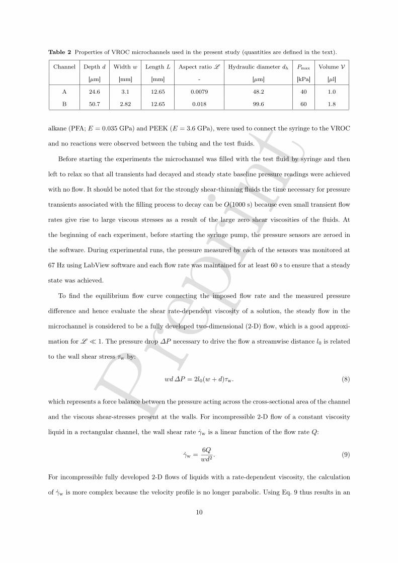
Table 2 Properties of VROC microchannels used in the present study (quantities are defined in the text).

Channel Depth d Width w Length L Aspect ratio L Hydraulic diameter dh Pmax Volume V

[µm] [mm] [mm] - [µm] [kPa] [µl]

A 24.6 3.1 12.65 0.0079 48.2 40 1.0

B 50.7 2.82 12.65 0.018 99.6 60 1.8

alkane (PFA; E = 0.035 GPa) and PEEK (E = 3.6 GPa), were used to connect the syringe to the VROC

and no reactions were observed between the tubing and the test fluids.

Before starting the experiments the microchannel was filled with the test fluid by syringe and then

left to relax so that all transients had decayed and steady state baseline pressure readings were achieved

with no flow. It should be noted that for the strongly shear-thinning fluids the time necessary for pressure

transients associated with the filling process to decay can be O(1000 s) because even small transient flow

rates give rise to large viscous stresses as a result of the large zero shear viscosities of the fluids. At

the beginning of each experiment, before starting the syringe pump, the pressure sensors are zeroed in

the software. During experimental runs, the pressure measured by each of the sensors was monitored at

67 Hz using LabView software and each flow rate was maintained for at least 60 s to ensure that a steady

state was achieved.

To find the equilibrium flow curve connecting the imposed flow rate and the measured pressure

difference and hence evaluate the shear rate-dependent viscosity of a solution, the steady flow in the

microchannel is considered to be a fully developed two-dimensional (2-D) flow, which is a good approxi-

mation for L 1. The pressure drop ∆P necessary to drive the flow a streamwise distance l0 is related

to the wall shear stress τw by:

wd∆P = 2l0(w + d)τw. (8)

which represents a force balance between the pressure acting across the cross-sectional area of the channel

and the viscous shear-stresses present at the walls. For incompressible 2-D flow of a constant viscosity

liquid in a rectangular channel, the wall shear rate γw is a linear function of the flow rate Q:

γw =6Qwd2

. (9)

For incompressible fully developed 2-D flows of liquids with a rate-dependent viscosity, the calculation

of γw is more complex because the velocity profile is no longer parabolic. Using Eq. 9 thus results in an

10

Prep

rint

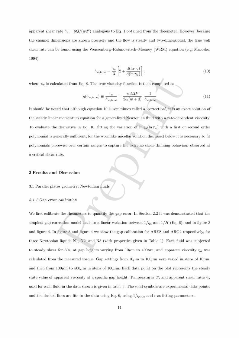
apparent shear rate γa = 6Q/(wd2) analogous to Eq. 1 obtained from the rheometer. However, because

the channel dimensions are known precisely and the flow is steady and two-dimensional, the true wall

shear rate can be found using the Weissenberg–Rabinowitsch–Mooney (WRM) equation (e.g. Macosko,

1994):

γw,true =γa

3

[2 +

d(ln γa)d(ln τw)

], (10)

where τw is calculated from Eq. 8. The true viscosity function is then computed as

η(γw,true) ≡τw

γw,true=

wd∆P

2l0(w + d)1

γw,true(11)

It should be noted that although equation 10 is sometimes called a ‘correction’, it is an exact solution of

the steady linear momentum equation for a generalized Newtonian fluid with a rate-dependent viscosity.

To evaluate the derivative in Eq. 10, fitting the variation of ln γa(ln τw) with a first or second order

polynomial is generally sufficient; for the wormlike micellar solution discussed below it is necessary to fit

polynomials piecewise over certain ranges to capture the extreme shear-thinning behaviour observed at

a critical shear-rate.

3 Results and Discussion

3.1 Parallel plates geometry: Newtonian fluids

3.1.1 Gap error calibration

We first calibrate the rheometers to quantify the gap error. In Section 2.2 it was demonstrated that the

simplest gap correction model leads to a linear variation between 1/ηa and 1/H (Eq. 6), and in figure 3

and figure 4. In figure 3 and figure 4 we show the gap calibration for ARES and ARG2 respectively, for

three Newtonian liquids N1, N2, and N3 (with properties given in Table 1). Each fluid was subjected

to steady shear for 30s, at gap heights varying from 10µm to 400µm, and apparent viscosity ηa was

calculated from the measured torque. Gap settings from 10µm to 100µm were varied in steps of 10µm,

and then from 100µm to 500µm in steps of 100µm. Each data point on the plot represents the steady

state value of apparent viscosity at a specific gap height. Temperatures T , and apparent shear rates γa

used for each fluid in the data shown is given in table 3. The solid symbols are experimental data points,

and the dashed lines are fits to the data using Eq. 6, using 1/ηtrue and ε as fitting parameters.

11

Prep

rint

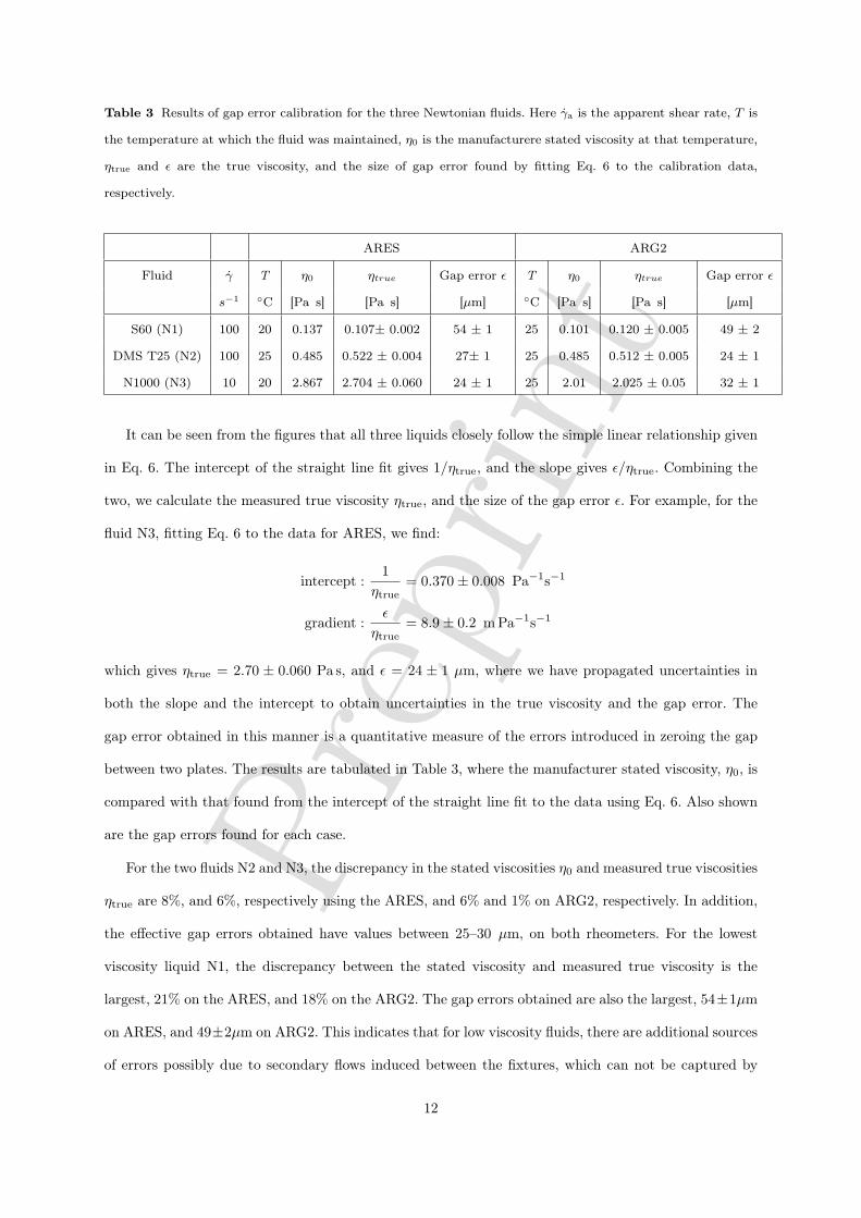
Table 3 Results of gap error calibration for the three Newtonian fluids. Here γa is the apparent shear rate, T is

the temperature at which the fluid was maintained, η0 is the manufacturere stated viscosity at that temperature,

ηtrue and ε are the true viscosity, and the size of gap error found by fitting Eq. 6 to the calibration data,

respectively.

ARES ARG2

Fluid γ T η0 ηtrue Gap error ε T η0 ηtrue Gap error ε

s−1 C [Pa s] [Pa s] [µm] C [Pa s] [Pa s] [µm]

S60 (N1) 100 20 0.137 0.107± 0.002 54 ± 1 25 0.101 0.120 ± 0.005 49 ± 2

DMS T25 (N2) 100 25 0.485 0.522 ± 0.004 27± 1 25 0.485 0.512 ± 0.005 24 ± 1

N1000 (N3) 10 20 2.867 2.704 ± 0.060 24 ± 1 25 2.01 2.025 ± 0.05 32 ± 1

It can be seen from the figures that all three liquids closely follow the simple linear relationship given

in Eq. 6. The intercept of the straight line fit gives 1/ηtrue, and the slope gives ε/ηtrue. Combining the

two, we calculate the measured true viscosity ηtrue, and the size of the gap error ε. For example, for the

fluid N3, fitting Eq. 6 to the data for ARES, we find:

intercept :1

ηtrue= 0.370± 0.008 Pa−1s−1

gradient :ε

ηtrue= 8.9± 0.2 m Pa−1s−1

which gives ηtrue = 2.70 ± 0.060 Pa s, and ε = 24 ± 1 µm, where we have propagated uncertainties in

both the slope and the intercept to obtain uncertainties in the true viscosity and the gap error. The

gap error obtained in this manner is a quantitative measure of the errors introduced in zeroing the gap

between two plates. The results are tabulated in Table 3, where the manufacturer stated viscosity, η0, is

compared with that found from the intercept of the straight line fit to the data using Eq. 6. Also shown

are the gap errors found for each case.

For the two fluids N2 and N3, the discrepancy in the stated viscosities η0 and measured true viscosities

ηtrue are 8%, and 6%, respectively using the ARES, and 6% and 1% on ARG2, respectively. In addition,

the effective gap errors obtained have values between 25–30 µm, on both rheometers. For the lowest

viscosity liquid N1, the discrepancy between the stated viscosity and measured true viscosity is the

largest, 21% on the ARES, and 18% on the ARG2. The gap errors obtained are also the largest, 54±1µm

on ARES, and 49±2µm on ARG2. This indicates that for low viscosity fluids, there are additional sources

of errors possibly due to secondary flows induced between the fixtures, which can not be captured by

12

Prep

rint

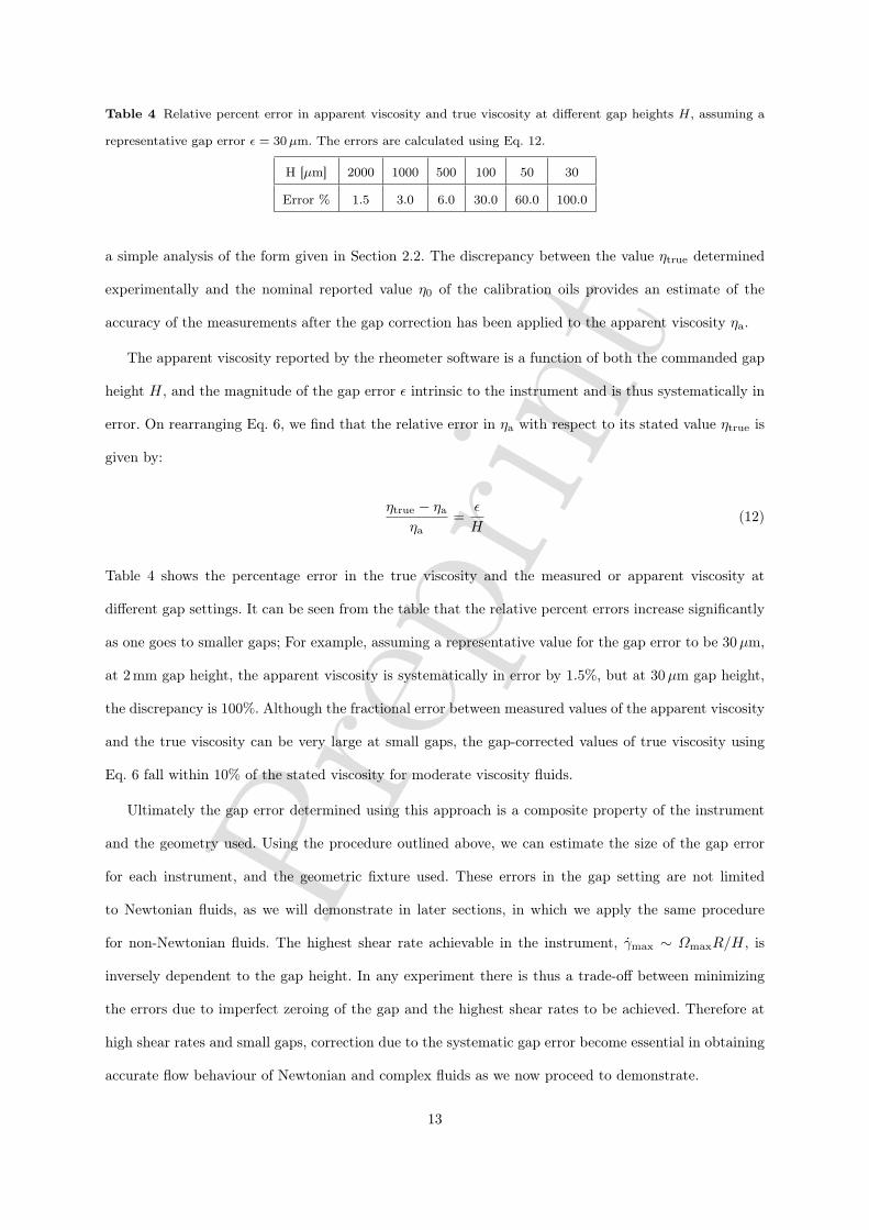
Table 4 Relative percent error in apparent viscosity and true viscosity at different gap heights H, assuming a

representative gap error ε = 30µm. The errors are calculated using Eq. 12.

H [µm] 2000 1000 500 100 50 30

Error % 1.5 3.0 6.0 30.0 60.0 100.0

a simple analysis of the form given in Section 2.2. The discrepancy between the value ηtrue determined

experimentally and the nominal reported value η0 of the calibration oils provides an estimate of the

accuracy of the measurements after the gap correction has been applied to the apparent viscosity ηa.

The apparent viscosity reported by the rheometer software is a function of both the commanded gap

height H, and the magnitude of the gap error ε intrinsic to the instrument and is thus systematically in

error. On rearranging Eq. 6, we find that the relative error in ηa with respect to its stated value ηtrue is

given by:

ηtrue − ηaηa

=ε

H(12)

Table 4 shows the percentage error in the true viscosity and the measured or apparent viscosity at

different gap settings. It can be seen from the table that the relative percent errors increase significantly

as one goes to smaller gaps; For example, assuming a representative value for the gap error to be 30µm,

at 2 mm gap height, the apparent viscosity is systematically in error by 1.5%, but at 30µm gap height,

the discrepancy is 100%. Although the fractional error between measured values of the apparent viscosity

and the true viscosity can be very large at small gaps, the gap-corrected values of true viscosity using

Eq. 6 fall within 10% of the stated viscosity for moderate viscosity fluids.

Ultimately the gap error determined using this approach is a composite property of the instrument

and the geometry used. Using the procedure outlined above, we can estimate the size of the gap error

for each instrument, and the geometric fixture used. These errors in the gap setting are not limited

to Newtonian fluids, as we will demonstrate in later sections, in which we apply the same procedure

for non-Newtonian fluids. The highest shear rate achievable in the instrument, γmax ∼ ΩmaxR/H, is

inversely dependent to the gap height. In any experiment there is thus a trade-off between minimizing

the errors due to imperfect zeroing of the gap and the highest shear rates to be achieved. Therefore at

high shear rates and small gaps, correction due to the systematic gap error become essential in obtaining

accurate flow behaviour of Newtonian and complex fluids as we now proceed to demonstrate.

13

Prep

rint

3.1.2 High shear rate measurements

In this section we describe the behaviour of Newtonian, and weakly shear thinning fluids at very high

shear-rates. Even for Newtonian fluids, the issue of ‘apparent shear-thinning behaviour’ at high shear-

rates is important (Dontula et al. (1999)). Do some ‘Newtonian liquids’ become shear thinning at high

enough shear rates, or is the apparent shear-thinning behaviour explained by some other mechanism such

as viscous heating. For the non-Newtonian case, particularly for worm-like micellar solutions, the high-

shear rate behaviour of the solution beyond the plateau in the flow curve remains unclear (Radulescu

et al., 2003).

We begin by describing results for Newtonian fluids. The three Newtonian fluids N1, N2, and N3,

were subjected to a steady shear ramp test on the ARES rheometer using a plate-plate geometry with

plate diameter 50 mm. The fluids were subjected to shear rates from 1 s−1 to 60000 s−1, in logarithmic

steps with 5 points per decade. Each shear step was maintained for 20 s. The commanded gap height

was set to 50 µm and the temperature at the lower plate was held fixed at 25C.

Figure 5 shows the plot of true viscosity with shear rate for the three nominally Newtonian fluids. The

true viscosity and the true shear rate were obtained from the apparent values reported by the software,

by correcting for the gap error, as described in Section 2.2. The gap error ε for the ARES rheometer

was found as described in Section 3.1.1. Once the gap error was known, Eq. 5 was used to calculate true

shear rate, and the gap-adjusted true viscosity using Eq. 6 in the form

ηtrue = ηa

(H + ε

H

)(13)

The solid symbols in the plot show the experimental data points. The two dashed lines running diagonally

across the plot represent the minimum and the maximum limiting values of the measurable torque. The

minimum and maximum torque values, for the force transducer used, are Tmin = 1.96× 10−4 N m, and

Tmax = 0.196N m, respectively. These torque limits correspond to minimum and maximum stress values

τmin = 7.989 N/m2, and τmax = 7989 N/m2, respectively for the 50 mm diameter plate (Eq. 3). Having

determined the minimum and maximum shear tresses, the range of viscosities and shear rates accessible

are related by the expressions:

ηmin =τmin

γtrue(14)

ηmax =τmax

γtrue(15)

14

Prep

rint

where the true shear rate is given by incorporating the gap error via Eq. 5.

The viscosity of each Newtonian fluid is constant for more than three decades in shear rate, up to

γ ≈ 104 s−1 . For the fluid N2 with viscosity η0 = 0.485 Pa s, there is a visible drop in viscosity beyond

shear rates of 20,000 s−1. We investigate this case of apparent shear thinning in further detail below.

At very high shear rates, there are several additional factors such as inertial effects, and viscous

heating that impact rheometric measurements (Bird et al., 1987; Macosko, 1994). At high rotation rates,

centrifugal stresses may become sufficiently large to overcome the surface tension stresses that hold

the liquid between the plates resulting in liquid being thrown out of the gap; a phenomenon termed

euphemistically the ‘radial migration effect’ (Connelly & Greener, 1985). Once the confined fluid is

partially ejected, the subsequent measurements are made with less fluid within the plates, which results

in a drop in measured torque, and hence in the viscosity. In particular, for a fluid with density ρ and

surface tension σ in a parallel plate geometry with plate radius R, rotating with angular velocity Ω, and

gap height H the centrifugal stresses overcome the surface tension stresses when (Tanner & Keentok,

1983; Connelly & Greener, 1985),

320

ρ (Ω2R2) >σ

H(16)

The critical apparent shear-rate at which the fluid begins to migrate outwards is given by rearranging

Eq. 16:

γapp,c =

(ΩR

H

)c

=

√20σ

3ρH3(17)

In addition, incorporating the gap error correction, we get:

γc =

√20σ

3ρ(H + ε)3(18)

Equation 18 shows that the critical shear rate for radial migration to occur decreases as gap height

increases (γc ∼ H−3/2). Thus the radial migration effect can be reduced by going to very small gap

heights. Furthermore, it is clear that a gap error results in a critical shear rate that is lower than the

predicted critical shear rate without correcting for the gap errors. For the fluid N2 (η0 = 0.485 Pa s),

the estimated critical shear rates at which the radial migration occurs at different gap heights (assuming

a gap error of 30 µm) are found to be γc = 8096 s−1 for H = 100 µm, γc = 16770 s−1 for H = 50 µm,

and γc = 29419 s−1 for H = 25 µm. It is noteworthy that these critical rates are within the range of

shear rates imposed in our experiments, and of the same order as the shear rates at which the viscosity

shows a noticeable drop. Many experimental and theoretical studies have shown that viscous heating

15

Prep

rint

can also significantly affect the flow properties of Newtonian fluids (Bird & Turian, 1962; Connelly &

Greener, 1985; Kramer et al., 1987; Rothstein & McKinley, 2001; Olagunju et al., 2002). In a previous

study (Ram, 1961), a drop in viscosity of water/glycerol solutions was reported and described as a shear-

thinning transition in an apparent Newtonian fluid at high shear rates. We re-examine this issue with

fluid N2, which shows a similar drop in viscosity at high shear rates. In addition to the radial migration

effect discussed above, it is possible that at very high shear rates there is sufficient viscous heating to

lower the viscosity of some fluids.

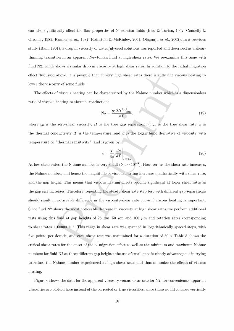
The effects of viscous heating can be characterized by the Nahme number which is a dimensionless

ratio of viscous heating to thermal conduction:

Na =η0βH

2γ2true

kT, (19)

where η0 is the zero-shear viscosity, H is the true gap separation, γtrue is the true shear rate, k is

the thermal conductivity, T is the temperature, and β is the logarithmic derivative of viscosity with

temperature or "thermal sensitivity", and is given by:

β =T

η0

∣∣∣∣∣ dηdT∣∣∣∣∣T=T0

. (20)

At low shear rates, the Nahme number is very small (Na ∼ 10−9). However, as the shear-rate increases,

the Nahme number, and hence the magnitude of viscous heating increases quadratically with shear rate,

and the gap height. This means that viscous heating effects become significant at lower shear rates as

the gap size increases. Therefore, repeating the steady shear rate step test with different gap separations

should result in noticeable difference in the viscosity-shear rate curve if viscous heating is important.

Since fluid N2 shows the most noticeable decrease in viscosity at high shear rates, we perform additional

tests using this fluid at gap heights of 25 µm, 50 µm and 100 µm and rotation rates corresponding

to shear rates 1–60000 s−1. This range in shear rate was spanned in logarithmically spaced steps, with

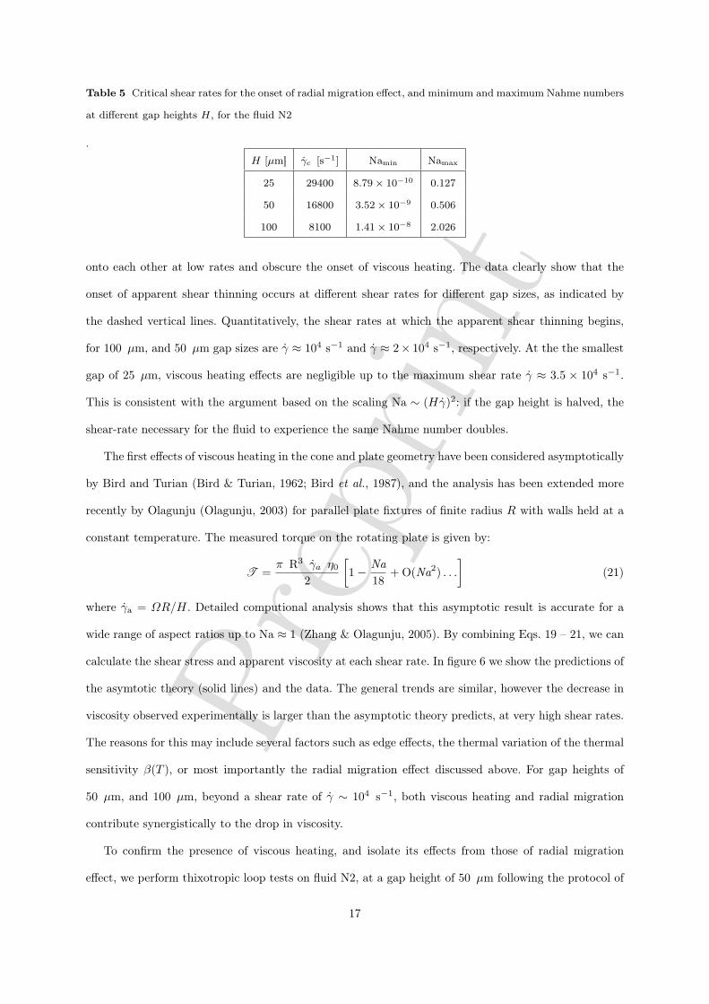
five points per decade, and each shear rate was maintained for a duration of 30 s. Table 5 shows the

critical shear rates for the onset of radial migration effect as well as the minimum and maximum Nahme

numbers for fluid N2 at three different gap heights: the use of small gaps is clearly advantageous in trying

to reduce the Nahme number experienced at high shear rates and thus minimize the effects of viscous

heating.

Figure 6 shows the data for the apparent viscosity versus shear rate for N2; for convenience, apparent

viscosities are plotted here instead of the corrected or true viscosities, since these would collapse vertically

16

Prep

rint

Table 5 Critical shear rates for the onset of radial migration effect, and minimum and maximum Nahme numbers

at different gap heights H, for the fluid N2

.

H [µm] γc [s−1] Namin Namax

25 29400 8.79× 10−10 0.127

50 16800 3.52× 10−9 0.506

100 8100 1.41× 10−8 2.026

onto each other at low rates and obscure the onset of viscous heating. The data clearly show that the

onset of apparent shear thinning occurs at different shear rates for different gap sizes, as indicated by

the dashed vertical lines. Quantitatively, the shear rates at which the apparent shear thinning begins,

for 100 µm, and 50 µm gap sizes are γ ≈ 104 s−1 and γ ≈ 2× 104 s−1, respectively. At the the smallest

gap of 25 µm, viscous heating effects are negligible up to the maximum shear rate γ ≈ 3.5 × 104 s−1.

This is consistent with the argument based on the scaling Na ∼ (Hγ)2: if the gap height is halved, the

shear-rate necessary for the fluid to experience the same Nahme number doubles.

The first effects of viscous heating in the cone and plate geometry have been considered asymptotically

by Bird and Turian (Bird & Turian, 1962; Bird et al., 1987), and the analysis has been extended more

recently by Olagunju (Olagunju, 2003) for parallel plate fixtures of finite radius R with walls held at a

constant temperature. The measured torque on the rotating plate is given by:

T =π R3 γa η0

2

[1− Na

18+ O(Na2) . . .

](21)

where γa = ΩR/H. Detailed computional analysis shows that this asymptotic result is accurate for a

wide range of aspect ratios up to Na ≈ 1 (Zhang & Olagunju, 2005). By combining Eqs. 19 – 21, we can

calculate the shear stress and apparent viscosity at each shear rate. In figure 6 we show the predictions of

the asymtotic theory (solid lines) and the data. The general trends are similar, however the decrease in

viscosity observed experimentally is larger than the asymptotic theory predicts, at very high shear rates.

The reasons for this may include several factors such as edge effects, the thermal variation of the thermal

sensitivity β(T ), or most importantly the radial migration effect discussed above. For gap heights of

50 µm, and 100 µm, beyond a shear rate of γ ∼ 104 s−1, both viscous heating and radial migration

contribute synergistically to the drop in viscosity.

To confirm the presence of viscous heating, and isolate its effects from those of radial migration

effect, we perform thixotropic loop tests on fluid N2, at a gap height of 50 µm following the protocol of

17

Prep

rint

Connelly & Greener (1985). In this test, fluid N2 was subjected to a stepped shear ramp from 1000 s−1

to 20000 s−1 in logarithmic steps, and then brought back down to 1000 s−1 in the same manner. The

duration of the thixotropic loop, tL, was varied from 4 s to 40 s. The maximum shear rate was chosen

using Eq. 17 and Table 5 such that no significant radial migration occurs. In a thixotropic loop test,

viscous heating is manifested in the form of hysteresis in the stress–strain-rate curve. If the area between

the ‘up’ and ‘down’ sweeps increases with loop time, it signifies greater viscous heating due to longer

duration of shearing. In figure 7, stress – strain-rate data for four different loop times tL = 4 s, 10 s,

20 s, 40 s are shown. For clarity the stress values for tL = 10 s, tL = 20 s, and tL = 40 s are shifted

vertically by 500 Pa, 1000 Pa and 2000 Pa, respectively. In agreement with Connelly & Greener (1985),

we observe that as the loop time is reduced, the hysteresis decreases. For the smallest loop time of 4 s

viscous heating is negligible, even for a maximum imposed shear rate γ = 20000 s−1.

To conclude, we have shown that modern rotational rheometers are capable of measuring accurate

viscometric proprties at high shear rates up to γ ∼ 5× 104 s−1 provided the gap heights are kept small.

Using the gap correction procedure outlined in section 2.2 accurate measurements of viscosity can be

obtained at least for constant viscosity Newtonian fluids. We have also shown that the effects of viscous

heating and centrifugal stresses can both be appreciable at high shear rates, and can manifest themselves

as apparent shear-thinning behaviour for nominally Newtonian fluids. In view of this, we now turn to

the use of micro-channel devices, which are not susceptible to the effects of either viscous heating or

centrifugal stresses.

3.2 Rectilinear flow of Newtonian fluids in micro-channels

Fundamentally, the VROC micro-channel device allows us to measure the pressure P (x, t) at various

streamwise locations along the centre of a straight channel for an imposed flow rate Q. The steady state

pressure as a function of streamwise location x for fluid N1 is shown in figure 8 at three different flow

rates 10 < Q ≤ 50 µl min−1. The pressure readings are sampled at 67 Hz and averaged over 10 s to

show the steady-state pressure for each flow rate. Fitting a first order polynomial shows that, as one

expects, for a given flow rate the streamwise pressure gradient dP/dx is constant for a straight channel

of uniform cross section.

18

Prep

rint

The transient pressure response to a step change in flow rate is illustrated clearly in figure 9: in these

tests, the fluid is initially at rest and then the syringe pump is started impulsively at time t = 0 s;

thereafter the commanded flow rate is reduced every 60 s. The pressure is sampled at 67 Hz and the

data output from the sensor software are treated with a moving average filter applied over 25 consecutive

samples. The pressure drop ∆P over the array of pressure sensors as a function of time is shown for two

different types of tubing, PFA (elastic modulus E ≈ 0.035 GPa) and PEEK (E ≈ 3.6 GPa) tubing. The

residual noise of the pressure sensor is approximately ±0.25% full scale of the sensor, corresponding to

±150 Pa for channel B, and limiting the lowest practical working pressure drop to approximately 300 Pa

where averaging over a large number of samples is required. However, much greater noise in the measured

pressure can be caused by periodic fluctuations in the flow rate from the syringe pump: at 50 µl min−1

the error is ±5% for the two sets of data with no bubble in the syringe. Fluctuations in flow rate can be

damped significantly by introducing a compliant air bubble into the syringe and in this case the error is

±1%. Hence it is important to average over a large number of samples to account for periodicity in the

flow rate from the syringe pump.

The transient response in the pressure difference to a step change of Q is clear and it is important

to wait for the signal to attain a steady state in order to calculate the equilibrium values of the pressure

difference ∆P . This transient response is highly dependent on any air bubbles in the system as well as

the viscosity of the fluid. For fluid N1 shown in figure 9, the transient pressure drop with an air bubble

present is well fitted by a decaying exponential with a time constant of 3 s, while with no bubbles in

the system the time constant is < 1 s. Therefore, to avoid long transient flows, it is important to ensure

that the syringe and tubing are free of bubbles. This is critical for the shear-thinning viscoelastic liquids

discussed in the following section where the time needed to reach a steady state may be O(1000 s)

depending on the flow rate.

In figure 10 we show that the pressure difference ∆P for the three constant viscosity liquids N1, N2,

and N3, is a linear function of flow rate Q passing through the origin as expected. At the highest flow rate

shown in figure 10, Q = 80 µl/min, the Reynolds number based on the hydraulic diameter of the channel

is Re = ρQdh/(ηwd) = 8× 10−3 indicating that the flow is dominated by viscous stresses and far from

the onset of any inertial effects or turbulence. The Nahme number (Eq. 19) describes the importance of

viscous heating, and using the properties listed in figure 1, we find for all flow rates Na < 10−4 for fluids

N1–3 indicating that viscous heating is insignificant even at the largest flow rates used in this work.

19

Prep

rint

Thus we consider equations 8 & 9 for the wall shear rate and wall shear stress to provide an accurate

description of the flow curve.

Viscosity data from VROC channel B for four constant viscosity fluids are shown in figure 11. The

scatter in the measured value of η(γ) is less than 5% and the measured viscosity is independent of

shear rate as expected. As we show in table 1, the data are in good agreement with the gap–corrected

measurements from the parallel-plate fixture using a standard rheometer. The upper and lower sensing

limits of the VROC channel B are indicated by the dashed lines in figure 11: in the parameter space

of viscosity and shear rate, a specified pressure drop ∆Pmin corresponds to a fixed minimum wall shear

stress (ηγ)min = τmin = wd∆Pmin/(2L(w+d)) from Eq. 8. This corresponds to a slope of −1 on a log-log

plot of viscosity versus shear rate. A similar analysis of course also applies for the maximum pressure

drop and thus for fluids with a lower viscosity, higher shear rates can be attained.

On the same figure, we show data for water; here we can clearly see the advantage the VROC offers

for low viscosity fluids, allowing shear rates 103 ≤ γ ≤ 105 s−1 to be obtained for shear viscosities

η ∼ 1 mPa s. For these measurements the Reynolds number is in the range 1 < Re < 100 which is still

significantly below the onset of turbulent flow in a channel Re = 2000. At the maximum shear rate of

γ = 8 × 104 s−1, the Nahme number Na < 10−3 and viscous heating is negligible even at these high

shear-rates.

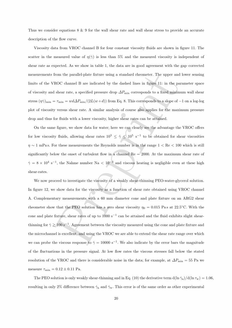
We now proceed to investigate the viscosity of a weakly shear-thinning PEO-water-glycerol solution.

In figure 12, we show data for the viscosity as a function of shear rate obtained using VROC channel

A. Complementary measurements with a 60 mm diameter cone and plate fixture on an ARG2 shear

rheometer show that the PEO solution has a zero shear viscosity η0 = 0.015 Pa s at 22.5C. With the

cone and plate fixture, shear rates of up to 1000 s−1 can be attained and the fluid exhibits slight shear-

thinning for γ ? 100 s−1. Agreement between the viscosity measured using the cone and plate fixture and

the microchannel is excellent, and using the VROC we are able to extend the shear rate range over which

we can probe the viscous response to γ = 10000 s−1. We also indicate by the error bars the magnitude

of the fluctuations in the pressure signal. At low flow rates the viscous stresses fall below the stated

resolution of the VROC and there is considerable noise in the data; for example, at ∆Pmin = 55 Pa we

measure τmin = 0.12± 0.11 Pa.

The PEO solution is only weakly shear-thinning and in Eq. (10) the derivative term d(ln γa)/d(ln τw) = 1.06,

resulting in only 2% difference between γa and γw. This error is of the same order as other experimental

20

Prep

rint

errors that we would expect due to fluctuations in temperature; imposed flow rate and the precision and

accuracy of the pressure transducers and it is sufficiently accurate to process the measurements for such

a weakly shear-thinning fluid in the same way for a Newtonian liquid.

In summary, we have seen how streamwise pressure measurements along a straight microfluidic chan-

nel allow us to calculate the viscosity for several Newtonian liquids and weakly shear thinning-liquids

over a wide range of shear rates. The measurements agree extremely well with data from a narrow gap

parallel-plate geometry and have the additional advantage that no fluid is ejected from the device due

to large rotation rates, and the flow remains in a low Reynolds number and low Nahme number regime.

3.3 Measurements of fluids with a shear-rate-dependent viscosity using parallel plates and

microchannels

In Sections 3.1 & 3.2 we have demonstrated two techniques for accurately measuring the shear viscosities

of Newtonian liquids at large shear rates by reducing the characteristic length scale of the device to l ∼

30− 50 µm. For weakly shear-thinning fluids the small shear–rate–dependent change in viscosity allows

the same analysis as for a constant viscosity liquid, to within experimental error. We now extend the

analysis to complex liquids with a strongly shear-rate-dependent viscosity. To investigate the possibilities

and limitations of the two techniques, we present results for an aqueous xanthan gum and a CPyCl/NaSal

micellar solution, which are both known a priori to have shear viscosities which change by several orders

of magnitude over certain shear-rate ranges. The xanthan gum solution is a strongly shear-thinning

liquid (Milas et al., 1990) while the micellar solution shows a yield-like behaviour at a critical shear

stress which is associated with the onset of shear-banding flow (Rehage & Hoffmann, 1991; Pipe et al.,

to be submitted).

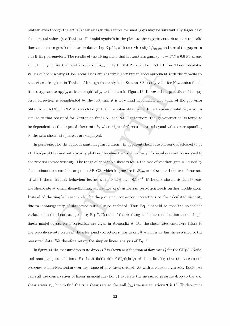
We first consider gap correction of measurements in a parallel-plate fixture with narrow gaps from

500 µm − 10 µm. The method for determining the gap error and the resulting analysis to obtain true

shear rates and viscosities remain the same as described in Section 2.2. In figure 13, we show gap error

calibration using aqueous xanthan gum and for the CPyCl/NaSal micellar solution using the ARG2.

Both fluids were subjected to steady shear for a duration of 60 s, at constant apparent shear rates of

γa = 1 s−1, and γa = 0.006 s−1, for CPyCl/NaSal micellar solution, and xanthan gum respectively. The

shear rates were chosen such that the viscometric response is expected to remain in the zero-shear rate

21

Prep

rint

plateau even though the actual shear rates in the sample for small gaps may be substantially larger than

the nominal values (see Table 4). The solid symbols in the plot are the experimental data, and the solid

lines are linear regression fits to the data using Eq. 13, with true viscosity 1/ηtrue, and size of the gap error

ε as fitting parameters. The results of the fitting show that for xanthan gum, ηtrue = 17.7±0.6 Pa s, and

ε = 31± 1 µm. For the micellar solution, ηtrue = 19.1± 0.4 Pa s, and ε = 53± 1 µm. These calculated

values of the viscosity at low shear rates are slightly higher but in good agreement with the zero-shear-

rate viscosities given in Table 1. Although the analysis in Section 2.2 is only valid for Newtonian fluids,

it also appears to apply, at least empirically, to the data in Figure 13. However interpretation of the gap

error correction is complicated by the fact that it is now fluid dependent. The value of the gap error

obtained with CPyCl/NaSal is much larger than the value obtained with xanthan gum solution, which is

similar to that obtained for Newtonian fluids N2 and N3. Furthermore, the ‘gap-correction’ is found to

be dependent on the imposed shear rate γa when higher deformation rates beyond values corresponding

to the zero shear rate plateau are employed.

In particular, for the aqueous xanthan gum solution, the apparent shear rate chosen was selected to be

at the edge of the constant viscosity plateau, therefore the ‘true viscosity’ obtained may not correspond to

the zero shear-rate viscosity. The range of applicable shear rates in the case of xanthan gum is limited by

the minimum measurable torque on AR-G2, which in practice is Tmin = 1.0µm, and the true shear rate

at which shear-thinning behaviour begins, which is at γtrue = 0.1 s−1. If the true shear rate falls beyond

the shear-rate at which shear-thinning occurs, the analysis for gap correction needs further modification.

Instead of the simple linear model for the gap error correction, corrections to the calculated viscosity

due to inhomogeneity of shear-rate must also be included. Thus Eq. 6 should be modified to include

variations in the shear-rate given by Eq. 7. Details of the resulting nonlinear modification to the simple

linear model of gap error correction are given in Appendix A. For the shear-rates used here (close to

the zero-shear-rate plateau) the additional correction is less than 5% which is within the precision of the

measured data. We therefore retain the simpler linear analysis of Eq. 6.

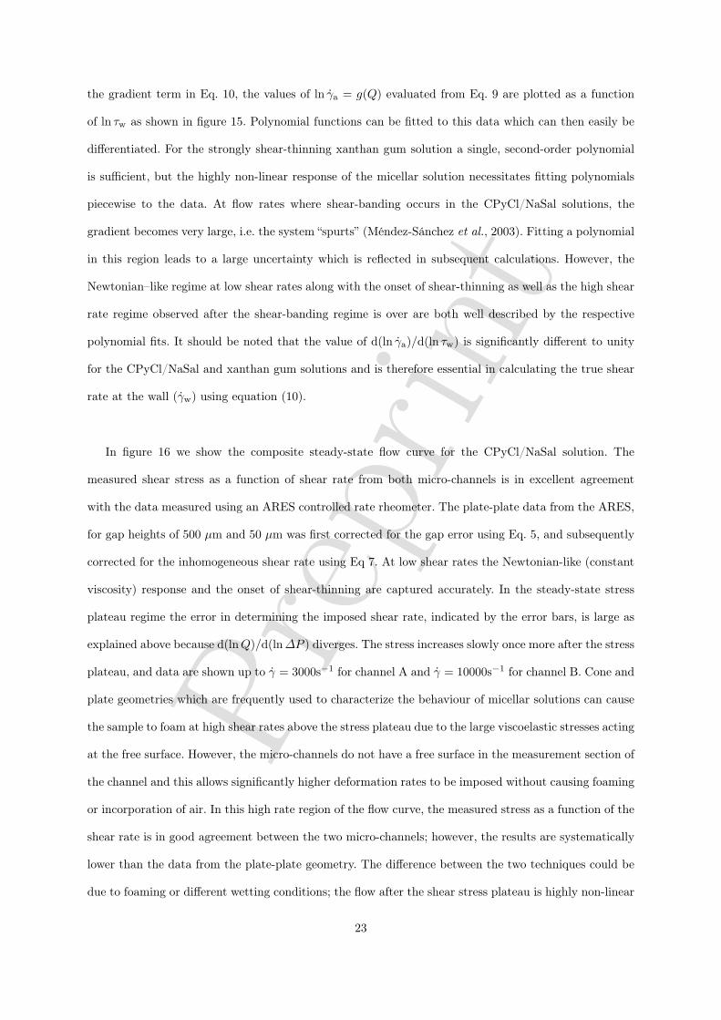
In figure 14 the measured pressure drop∆P is shown as a function of flow rate Q for the CPyCl/NaSal

and xanthan gum solutions. For both fluids d(ln∆P )/d(lnQ) 6= 1, indicating that the viscometric

response is non-Newtonian over the range of flow rates studied. As with a constant viscosity liquid, we

can still use conservation of linear momentum (Eq. 8) to relate the measured pressure drop to the wall

shear stress τw, but to find the true shear rate at the wall (γw) we use equations 9 & 10. To determine

22

Prep

rint

the gradient term in Eq. 10, the values of ln γa = g(Q) evaluated from Eq. 9 are plotted as a function

of ln τw as shown in figure 15. Polynomial functions can be fitted to this data which can then easily be

differentiated. For the strongly shear-thinning xanthan gum solution a single, second-order polynomial

is sufficient, but the highly non-linear response of the micellar solution necessitates fitting polynomials

piecewise to the data. At flow rates where shear-banding occurs in the CPyCl/NaSal solutions, the

gradient becomes very large, i.e. the system “spurts” (Méndez-Sánchez et al., 2003). Fitting a polynomial

in this region leads to a large uncertainty which is reflected in subsequent calculations. However, the

Newtonian–like regime at low shear rates along with the onset of shear-thinning as well as the high shear

rate regime observed after the shear-banding regime is over are both well described by the respective

polynomial fits. It should be noted that the value of d(ln γa)/d(ln τw) is significantly different to unity

for the CPyCl/NaSal and xanthan gum solutions and is therefore essential in calculating the true shear

rate at the wall (γw) using equation (10).

In figure 16 we show the composite steady-state flow curve for the CPyCl/NaSal solution. The

measured shear stress as a function of shear rate from both micro-channels is in excellent agreement

with the data measured using an ARES controlled rate rheometer. The plate-plate data from the ARES,

for gap heights of 500 µm and 50 µm was first corrected for the gap error using Eq. 5, and subsequently

corrected for the inhomogeneous shear rate using Eq 7. At low shear rates the Newtonian-like (constant

viscosity) response and the onset of shear-thinning are captured accurately. In the steady-state stress

plateau regime the error in determining the imposed shear rate, indicated by the error bars, is large as

explained above because d(lnQ)/d(ln∆P ) diverges. The stress increases slowly once more after the stress

plateau, and data are shown up to γ = 3000s−1 for channel A and γ = 10000s−1 for channel B. Cone and

plate geometries which are frequently used to characterize the behaviour of micellar solutions can cause

the sample to foam at high shear rates above the stress plateau due to the large viscoelastic stresses acting

at the free surface. However, the micro-channels do not have a free surface in the measurement section of

the channel and this allows significantly higher deformation rates to be imposed without causing foaming

or incorporation of air. In this high rate region of the flow curve, the measured stress as a function of the

shear rate is in good agreement between the two micro-channels; however, the results are systematically

lower than the data from the plate-plate geometry. The difference between the two techniques could be

due to foaming or different wetting conditions; the flow after the shear stress plateau is highly non-linear

23

Prep

rint

(Pipe et al., to be submitted), and the interaction of velocity fluctuations and interfacial tension may

play a role in determining the flow established in this regime.

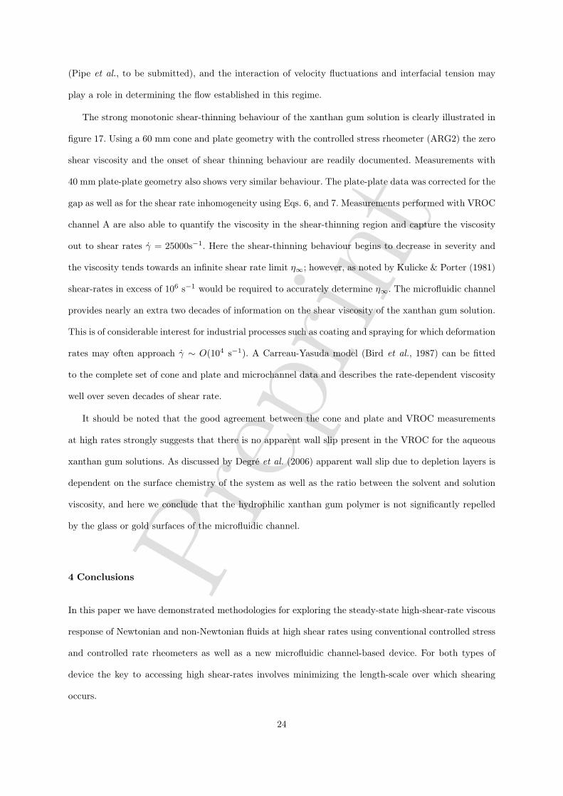
The strong monotonic shear-thinning behaviour of the xanthan gum solution is clearly illustrated in

figure 17. Using a 60 mm cone and plate geometry with the controlled stress rheometer (ARG2) the zero

shear viscosity and the onset of shear thinning behaviour are readily documented. Measurements with

40 mm plate-plate geometry also shows very similar behaviour. The plate-plate data was corrected for the

gap as well as for the shear rate inhomogeneity using Eqs. 6, and 7. Measurements performed with VROC

channel A are also able to quantify the viscosity in the shear-thinning region and capture the viscosity

out to shear rates γ = 25000s−1. Here the shear-thinning behaviour begins to decrease in severity and

the viscosity tends towards an infinite shear rate limit η∞; however, as noted by Kulicke & Porter (1981)

shear-rates in excess of 106 s−1 would be required to accurately determine η∞. The microfluidic channel

provides nearly an extra two decades of information on the shear viscosity of the xanthan gum solution.

This is of considerable interest for industrial processes such as coating and spraying for which deformation

rates may often approach γ ∼ O(104 s−1). A Carreau-Yasuda model (Bird et al., 1987) can be fitted

to the complete set of cone and plate and microchannel data and describes the rate-dependent viscosity

well over seven decades of shear rate.

It should be noted that the good agreement between the cone and plate and VROC measurements

at high rates strongly suggests that there is no apparent wall slip present in the VROC for the aqueous

xanthan gum solutions. As discussed by Degré et al. (2006) apparent wall slip due to depletion layers is

dependent on the surface chemistry of the system as well as the ratio between the solvent and solution

viscosity, and here we conclude that the hydrophilic xanthan gum polymer is not significantly repelled

by the glass or gold surfaces of the microfluidic channel.

4 Conclusions

In this paper we have demonstrated methodologies for exploring the steady-state high-shear-rate viscous

response of Newtonian and non-Newtonian fluids at high shear rates using conventional controlled stress

and controlled rate rheometers as well as a new microfluidic channel-based device. For both types of

device the key to accessing high shear-rates involves minimizing the length-scale over which shearing

occurs.

24

Prep

rint

Using the conventional rotational rheometers it is important to accurately calibrate the errors incurred

in zeroing the gap when narrow gaps (H > 250 µm) are employed. We have demonstrated that the simple

linear approach proposed by Connelly and Greener can be used to evaluate gap errors and correct the

apparent viscosities obtained at different gaps to obtain true viscosities. We have implemented this

approach for both Newtonian and non-Newtonian fluids, and demonstrated that the method works

surprisingly well for both. We observe that for moderate viscosity Newtonian fluids N2 and N3, the true

viscosities calculated via gap-calibration (Eq. 6) are within 7% of the stated zero-shear viscosities. The

systematic gap offset errors obtained with these two fluids, are ε ≈ 30 µm, for both rheometers used.

The lowest viscosity Newtonian fluid N1 shows significant deviation from these values. This may be due,

at least partially, to larger levels of noise in the data at the lower torque limits of the instrument but it

serves to remind us that this approximate gap correction approach involves both the geometry and the

test fluid. In the case of non-Newtonian fluids, we have demonstrated that the same linear approximate

correction works, although not uniformly well. The gap error calibration approach for the viscous aqueous

xanthan gum yields values for the gap error consistent with the two Newtonian fluids N2, and N3, but

the gap error obtained with a strongly shear thinning micellar solution yields higher values similar to

those measured for the low viscosity Newtonian fluid N1. Thus the approach is valid for both Newtonian

and non-Newtonian fluids, but with differing (and a priori) unknown accuracy.

We also studied the high shear-rate behaviour of Newtonian and non-Newtonian fluids. To achieve

high shear rates using conventional rheometers, very small gap heights (H < 100 µm) must be used,

leading to increased differences between the apparent viscosities and true viscosities (see Table 4), and it

is essential to correct for gap errors. Using such protocols may lead to apparent shear-thinning behaviour

even in Newtonian calibration oils. We identified two key systematic sources of error which could account

for these observations; radial migration and viscous heating. Relevant dimensionless scalings show that

both effects become important in the vicinity of shear rates 104–105 s−1.

We have also investigated the viscous response of Newtonian and non-Newtonian fluids in straight

microfluidic channels. For constant viscosity liquids we are able to measure η0 over two and a half decades

of shear-rate, with the shear-rates attainable dependent on the viscosity of the fluid. For any given fluid

there are resolution limits associated with the resolution of the pressure sensor, and while at the highest

shear rates the percentage error is O(±0.25%), the error at the very lowest shear-rates is O(±50%),

although this can be reduced by sampling over longer times to determine an appropriate mean value.

25

Prep

rint

Additional errors in the measured steady-state viscosity can be introduced by the syringe/syringe pump

set-up. To ensure that these errors are small (< 5%) is is important to select a combination of syringe and

syringe pump which can provide a steady and constant flow at the desired flow rate. In our experimental

set-up this constraint limits measurements of high zero-shear-rate viscosity liquids at low shear rates due

to the difficutly in imposing very low flow rates with sufficient accuracy. Step changes in applied flow

rate lead to transient pressure drops in the microchannel and we associate this with the stiffness of the

tubing between the channel and the syringe and also at the channel exit. It is especially important to

reduce flow transients when using highly shear-thinning liquids and we show that a transient pressure

response with a time constant < 1 s can be obtained by using stiff PEEK tubing.

At moderate shear rates O(100 s−1), the measured viscosities of Newtonian calibration oils N1-3 are

in excellent agreement with those obtained from conventional rheometers. Shear rates O(104 s−1) can be

obtained using lower zero-shear-viscosities liquids and the viscosity of water was measured up to a shear

rate of 8× 104 s−1. The viscosities of two highly shear-thinning fluids calculated using the Weissenburg-

Rabinowitsch-Mooney equation (Eq. 10) were also found to be in good agreement with results from cone

and plate measurements and the effective shear-rate range that can be accessed is significantly increased

due to the decrease in viscosity associated with increasing shear-rate. Thus we were able to characterize

the viscosity of an aqueous xanthan gum solution up to γ = 30000 s−1 and capture the approach to the

infinite-shear-rate viscosity. Furthermore, for a shear banding worm-like micellar liquid we have been able

to explore the steady-state flow curve up to γ = 10000 s−1, charting the viscous response at shear-rates

significantly beyond the end of the shear-stress plateau.

The results presented here show that both conventional rheometry, and micro-channel rheometry have

their specific domains of applicability. To access high shear rates, both viscometric approaches can be

used, but each has particular strengths and weaknesses. In rotational rheometers, the effects of centrifugal

stresses, and viscous heating can be significant. Viscous heating effects can be substantially reduced by

applying shear ramps in a very short interval of time. Radial migration effects can be mitigated by

moving to very small gaps but the resulting systematic gap error grows. In addition, the magnitude of

the gap correction that must be applied to the measured data appears to be dependent on the viscosity

of the fluids under investigation.

Microfluidic-based rheometry offers several distinct advantages over conventional rheometry. We have

demonstrated that high shear rates can be achieved using the micro-channels while still minimizing

26

Prep

rint

inertial and viscous heating effects, avoiding the need for an ad hoc correction. On the other hand, the

dynamic range of the pressure transducers mounted on the micro-channels constrains the range of fluid

viscosities that can be effectively studied. For constant viscosity fluids with a zero-shear-rate viscosity

upwards of 1 Pa s, the applicability of the technique is also limited by the range of flow rates that can

be reached by the syringe and syringe pump set-up.

Important questions thus arise with regard to the optimal choice of rheometer for investigating the

high shear-rate viscometry of a given fluid. To assess which approach is more suitable, it is helpful to have

a picture of the operating space in terms of the fluid viscosities and the range of shear rates achievable

for each class of device, and compare and contrast them. In Figure 18, we show the relevant operating

spaces in terms of viscosity and shear rate, for a microfluidic channel (fig. 18a), and a controlled strain

device (ARES) with typical fixture settings (fig. 18b). The lines 1 and 2 in figure 18a represent the lower

and upper bounds for the VROC channel B based on the minimum and maximum measurable pressure

difference ∆P. According to Eq. 8, the measured pressure difference is directly related to the wall stress,

and the apparent shear rate is directly related to the volume flow rate by Eq. 9. Thus, for the limiting

values of minimum and maximum measurable pressure difference, we get:

τw,min =wd∆Pmin

2l0(w + d), τw,max =

wd∆Pmax

2l0(w + d). (22)

Combining Eq. 22 with the relation τ = ηγ gives two limiting curves of the form:

ηmin =τw,min

γw(23)

ηmax =τw,max

γw(24)

These lines are power laws of slope -1 on a log-log plot. For the VROC channel B with the minimum and

maximum pressure difference given in Table 2, we find τmin = 0.8 Pa, and τmax = 160.0 Pa. Another

important limiting case arises when the flow rate in the slit is so large that the Reynolds number for the

fully developed viscous flow in the channel exceeds Re ≡ ρQdh/(ηwd) = 2000. In this limit, the onset of

turbulence results in non–viscometric flow although it should be noted that some studies in microfluidic

channels (Peng et al., 1994) suggest that the turbulent transition may happen considerably earlier at

Re ≈ 200. Using Eq. 9, we can cast the expression for the critical Reynolds number in terms of the shear

rate and viscosity relation at which Re = 2000:

2000 =ρ dh d γw

6η(25)

27

Prep

rint

which gives:

(γw)crit =12000 ηρ dh d

. (26)

At the other extreme, a minimum attainable flow rate limited by the choice of syringe and the syringe

pump sets a lower cut-off for the shear rate based on Eq. 9, which in this case is γmin = 0.014 s−1, for

the minimum flow rate of Qmin = 1× 10−3 µl/min.

Analogously, we obtain the limiting curves, and hence operating space for a conventional rheometer

such as the ARES as shown in Figure 18b. Lines 1 and 2 represent the limit curves based on the minimum

and maximum measurable torques of the transducer. These limiting curves are the same as those given

by Eq. 15, and are of the form ηmin = τmin/γ, and ηmax = τmax/γ. Based on the minimum and maximum

torques Tmin = 1.96 × 10−4 N m, and Tmax = 0.196 N m, the values of the minimum and maximum

shear stress are τmin = 7.989 Pa, and τmax = 7989 Pa for a parallel-plate fixture of radius R = 25

mm. Again, these are power-laws with a slope of -1. The vertical line 3 is the high shear rate cutoff at

γ = 2 × 104 s−1, based on the onset of radial migration (Eq. 17) and viscous heating (Eq. 19) for a

typical gap height of 50 µm. As the gap spacing is increased, this limit shifts to lower shear-rates (see

Eq. 18). The vertical line 4 is a low shear rate cutoff constrained by the minimum achievable rotation

rate of the plate. The minimum rotation rate of the ARES motor is Ω = 2 × 10−6 rad s−1, and the

minimum achievable shear rate is given by γmin = RΩmin/H, which for a plate of radius R = 25 mm,

and a typical gap height H = 50 µm, gives γmin = 0.001 s−1.

These operating space diagrams show the range of shear rates that can be accessed for Newtonian

fluids and shear-thinning fluids of differing viscosities. For the VROC, the viscosity scale spans 7 orders

of magnitude from η = 10−5 Pa s to η = 102 Pa s, whereas for the ARES, the viscosity scale spans 9

orders of magnitude, but from η = 10−3 Pa s to η = 106 Pa s. This points to one important difference

between the two approaches: for high viscosity liquids, a conventional modern rheometer typically offers

a broader dynamic range compared to the solid state pressure sensors in the microfluidic channel. For

example, if the fluid has a zero shear viscosity of 10 Pa s, for the VROC the minimum and maximum

shear rates applicable are γmin = 0.1 s−1 and γmax = 20 s−1, respectively, whereas using the ARES

with a plate-plate fixture of radius R = 25 mm and gap height H = 50 µm, the minimum and the

maximum shear rates are γmin = 1 s−1 and γmin = 1000 s−1, respectively. On the other hand, inertial

effects are significant for low viscosity fluids using the ARES rheometer, severely constraining the useful

28

Prep

rint

range at high shear rates, while the lowest measurable torque limit curtails the accessible shear-rates at

the low shear-rate end. For a fluid with zero shear viscosity of 0.001 Pa s (1 cPs), the dynamic range of

shear-rate for the microfluidic device VROC is from γmin = 1000 s−1 to γmax = 200000 s−1, whereas

for the ARES the effective range with a gap of 50 µm is from γmin = 8000 s−1 to γmax = 20000 s−1.

Furthermore it should be noted that the Weissenberg–Rabinowitsch–Mooney equation (Eq. 10) can

be applied robustly to any pressure-flow-rate relationship obtained in the microfluidic device. By con-

trast, the simple linear gap correction applied to the narrow gap results for the parallel plates device

is strictly applicable only to Newtonian fluid data. Our measurements suggest that a simple gap-error

calibration can be applied to measurements with more complex shear thinning fluids; however, the gap

offset correction ε is both gap- and fluid-dependent. Ideally, to confirm the applicability of the simple

linear gap correction algorithm for a given fluid it is necessary to compare the gap-corrected data with

a direct measure of the true shear-rate-dependent material functions, obtained for example using the

microfluidic channel.

The flexibility of microfludic fabrication technologies also enables a wide range of different flow

channel configurations to be considered. Having demonstrated the efficacy of a simple rectilinear slit

device to determine flow curves for a range of complex fluids up to shear rates of 105 s−1, we hope in

the future to use this robust pressure-sensing technology to also measure entrance pressure drops and

planar elongational viscosities using other rheometer-on-a-chip designs.

Acknowledgements

The authors would like to thank Dr. S.-G. Baek and Dr. M. Yi of Rheosense, Inc. for providing us with

prototype microchannel designs. This research was supported in part by NASA (grant NNC04GA41G),

NSF (DMS DMS-0406590) and a gift from the Procter and Gamble company.

APPENDIX

In this appendix we outline the difficulties in adapting the expression for the shear-rate-dependent

viscosity measured using a parallel plates device (Eq. 7):

ηtrue(γtrue) =T /2πR3

γtrue

[3 +

d(ln T /2πR3)d(ln γtrue)

], (A-1)

29

Prep

rint

to include the linear gap error analysis of Connelly and Greener. We start by noting that the analysis

can follow two distinct approaches: one to find the gap error ε where the apparent shear rate γa is held

constant and the gap height H is altered, and the other to find the true shear-rate-dependent viscosity

where the gap height H is held constant and the shear rate or rotation rate is altered.

Where possible the analysis to find the gap height error ε should be performed in the zero-shear-

rate region so that the fluid viscosity is not a function of applied shear rate. However, for fluids which

start shear-thinning at very low shear-rates this can result in measured stresses below the resolution

of the rheometer torque transducer and it is not possible to access this region. In this case, we expect

the apparent viscosity to be a function of both the true shear-rate and the gap setting and we want to

find the gap error ε as a function of the apparent shear rate γa = ΩR/H which can be commanded in

software. We start from expression for the the true shear-rate γtrue = ΩR/(H + ε):

γtrue = γa

(H

H + ε

), (A-2)

and differentiating using the chain rule we find:

dγtrue

dγa

∣∣∣∣Ω

=(∂γtrue

∂H

)Ω

dHdγa

=(

H

H + ε

)2

. (A-3)

Thus we can re-write Eq. A-1 in terms of the apparent shear-rate:

ηtrue =T /2πR3

γa

(H + ε

H

)[3 +

(H

H + ε

)d(ln T /2πR3)

d(ln γa)

∣∣∣∣Ω

]. (A-4)

To solve for the gap error ε, we cast Eq. A-4 in terms of the apparent viscosity ηa (c.f. Eq. 6):

1ηa

=1

ηtrue

(1 +

ε

H

) 14

[3 +

(1

1 + ε/H

)d(ln T /2πR3)

d(ln γa)

∣∣∣∣Ω

], (A-5)

and we note that for a complex liquid outside the zero-shear-viscosity regime 1/ηa is a non-linear function

of 1/H. For a Newtonian viscous response in which τ ∼ γa, we recover Eq. 6 and 1/ηa varies linearly

with 1/H.

We now turn to the case where we wish to determine the shear-rate-dependent viscosity as a function

of the apparent shear-rate for a fixed gap height and known gap error. In this instance:

dγtrue

dγa

∣∣∣∣H

=(∂γtrue

∂Ω

)H

dΩdγa

=(

H

H + ε

), (A-6)

and for measurements performed over a range of rotation rates at a fixed gap height, Eq. A-1 becomes

(c.f. Eq. 7):

ηtrue(γtrue) = ηa(1 +

ε

H

) 14

[3 +

d(ln T /2πR3)d(ln γa)

∣∣∣∣H

]. (A-7)

30

Prep

rint

It is therefore clear that for shear-thinning fluids slightly different results can be obtained depending

on whether measurements are performed at constant gap (varying rotation rate) or constant rotation

rate (and varying the shear-rate by changing the gap). It is instructive to compare the magnitude of the

leading order correction due to (a) the error in gap height ε and (b) the derivative of the logarithmic

term due to a shear-rate-dependent viscosity. At small gaps H ∼ 50 µm, ε ∼ 30 µm and the correction

provided by the gap correction term in Eq. A-7 can be O(100%). On the other hand, the corrections

associated with the shear-thinning term in square brackets are much smaller. At low apparent shear-rates

a ratio of Eq. A-5 or Eq. A-7 with the linear form of Eq. 6 in the text show that the results in Eqs. A-5

& A-7 differ by at most [3 + (1 + ε/H)−1]/4. In the case of an extremely shear-thinning fluid in which

d(ln T /2πR3)d(ln γa)

→ 0,

both Eqs. A-5 & A-7 approach the same limit and the additional correction to the viscosity is only 25%.

Given that the majority of fluids do not shear-thin this strongly, the additional error due to a shear-rate-

dependent viscosity in many cases will be less than 10% of that due to gap-error. Thus we conclude that

in the majority of experiments applying the gap-error analysis alone will provide a good estimate of the

shear-rate-dependent viscosity.

References

Baek, S. G. & Magda, J. J. 2003 Monolithic rheometer plate fabricated using silicon micromachining

technology and containing miniature pressure sensors for n1 and n2 measurements. J. Rheol. 47 (5),

1249–1260.

Bird, R. B., Armstrong, R. C. & Hassager, O. 1987 Dynamics of Polymeric Liquids, vol 1 , 2nd

edn. John Wiley and Sons.

Bird, R. B. & Turian, R. M. 1962 Viscous heating effects in a cone and plate viscometer. Chem.

Eng. Sci. 17 (5), 331–334.

Clasen, C., Gearing, B. P. & McKinley, G. H. 2006 The flexure-based microgap rheometer

(FMR). Journal of Rheology. 6 (50), 883–905.

Clasen, C. & McKinley, G. H. 2004 Gap-depedent microrheometry of complex liquids. J. Non-

Newtonian Fluid Mech. 124, 1–10.

31

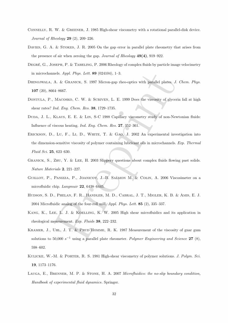
Prep

rint

Connelly, R. W. & Greener, J. 1985 High-shear viscometry with a rotational parallel-disk device.

Journal of Rheology 29 (2), 209–226.

Davies, G. A. & Stokes, J. R. 2005 On the gap error in parallel plate rheometry that arises from

the presence of air when zeroing the gap. Journal of Rheology 49(4), 919–922.

Degré, G., Joseph, P. & Tabeling, P. 2006 Rheology of complex fluids by particle image velocimetry

in microchannels. Appl. Phys. Lett. 89 (024104), 1–3.

Dhinojwala, A. & Granick, S. 1997 Micron-gap rheo-optics with parallel plates. J. Chem. Phys.

107 (20), 8664–8667.

Dontula, P., Macosko, C. W. & Scriven, L. E. 1999 Does the viscosity of glycerin fall at high

shear rates? Ind. Eng. Chem. Res. 38, 1729–1735.

Duda, J. L., Klaus, E. E. & Lin, S-C 1988 Capillary viscometry study of non-Newtonian fluids:

Influence of viscous heating. Ind. Eng. Chem. Res. 27, 352–361.

Erickson, D., Lu, F., Li, D., White, T. & Gao, J. 2002 An experimental investigation into

the dimension-sensitive viscosity of polymer containing lubricant oils in microchannels. Exp. Thermal

Fluid Sci. 25, 623–630.

Granick, S., Zhu, Y. & Lee, H. 2003 Slippery questions about complex fluids flowing past solids.

Nature Materials 2, 221–227.

Guillot, P., Panizza, P., Joanicot, J.-B. Salmon M. & Colin, A. 2006 Viscosimeter on a

microfluidic chip. Langmuir 22, 6438–6445.

Hudson, S. D., Phelan, F. R., Handler, M. D., Cabral, J. T., Migler, K. B. & Amis, E. J.

2004 Microfluidic analog of the four-roll mill. Appl. Phys. Lett. 85 (2), 335–337.

Kang, K., Lee, L. J. & Koelling, K. W. 2005 High shear microfluidics and its application in

rheological measurement. Exp. Fluids 38, 222–232.

Kramer, J., Uhl, J. T. & Prud’Homme, R. K. 1987 Measurement of the viscosity of guar gum

solutions to 50,000 s−1 using a parallel plate rheometer. Polymer Engineering and Science 27 (8),

598–602.

Kulicke, W.-M. & Porter, R. S. 1981 High-shear viscometry of polymer solutions. J. Polym. Sci.

19, 1173–1176.

Lauga, E., Brenner, M. P. & Stone, H. A. 2007 Microfluidics: the no-slip boundary condition,

Handbook of experimental fluid dynamics . Springer.

32

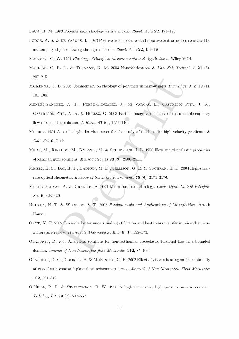
Prep

rint

Laun, H. M. 1983 Polymer melt rheology with a slit die. Rheol. Acta 22, 171–185.

Lodge, A. S. & de Vargas, L. 1983 Positive hole pressures and negative exit pressures generated by

molten polyethylene flowing through a slit die. Rheol. Acta 22, 151–170.

Macosko, C. W. 1994 Rheology: Principles, Measurements and Applications . Wiley-VCH.

Marrian, C. R. K. & Tennant, D. M. 2003 Nanofabrication. J. Vac. Sci. Technol. A 21 (5),

207–215.

McKenna, G. B. 2006 Commentary on rheology of polymers in narrow gaps. Eur. Phys. J. E 19 (1),

101–108.

Méndez-Sánchez, A. F., Pérez-González, J., de Vargas, L., Castrejón-Pita, J. R.,

Castrejón-Pita, A. A. & Huelsz, G. 2003 Particle image velocimetry of the unstable capillary

flow of a micellar solution. J. Rheol. 47 (6), 1455–1466.

Merrill 1954 A coaxial cylinder viscometer for the study of fluids under high velocity gradients. J.

Coll. Sci. 9, 7–19.

Milas, M., Rinaudo, M., Knipper, M. & Schuppiser, J. L. 1990 Flow and viscoelastic properties

of xanthan gum solutions. Macromolecules 23 (9), 2506–2511.

Mriziq, K. S., Dai, H. J., Dadmun, M. D., Jellison, G. E. & Cochran, H. D. 2004 High-shear-

rate optical rheometer. Reviews of Scientific Instruments 75 (6), 2171–2176.

Mukhopadhyay, A. & Granick, S. 2001 Micro- and nanorheology. Curr. Opin. Colloid Interface

Sci. 6, 423–429.

Nguyen, N.-T. & Wereley, S. T. 2002 Fundamentals and Applications of Microfluidics . Artech

House.

Obot, N. T. 2002 Toward a better understanding of friction and heat/mass transfer in microchannels–

a literature review. Microscale Thermophys. Eng. 6 (3), 155–173.

Olagunju, D. 2003 Analytical solutions for non-isothermal viscoelastic torsional flow in a bounded

domain. Journal of Non-Newtonian fluid Mechanics 112, 85–100.

Olagunju, D. O., Cook, L. P. & McKinley, G. H. 2002 Effect of viscous heating on linear stability

of viscoelastic cone-and-plate flow: axisymmetric case. Journal of Non-Newtonian Fluid Mechanics

102, 321–342.

O’Neill, P. L. & Stachowiak, G. W. 1996 A high shear rate, high pressure microviscometer.

Tribology Int. 29 (7), 547–557.

33

Prep

rint

Peng, X. F., Peterson, G. P. & Wang, B. X. 1994 Frictional flow characteristics of water flowing

through rectangular microchannels. Exp. Heat Transfer 7 (4), 249 – 264.

Pipe, C. J., Kim, N. J., McKinley, G. H., Vasquez, P. A. & Cook, L. P. to be submitted

Wormlike micellar solutions II: comparison between experimental data and scission model predictions.

J. Non-Newtonian Fluid Mech. submitted.

Radulescu, O., D., Olmsted P., P., Decruppe J., S., Lerouge, F., Berret J. & G., Porte

2003 Time scales in shear banding of wormlike micelles. Europhysics Letters 62 (2), 230–236.

Ram, A. 1961 High-Shear Viscometry of Polymer Solutions. Sc.D. Thesis. Massacusetts Institute of

Technology, Boston, MA.

Rehage, H. & Hoffmann, H. 1991 Viscoelastic surfactant solutions: model systems for rheological

research. Molecular Physics 74 (5), 933–973.

Rothstein, J. & McKinley, G. H. 2001 Non-isothermal modification of purely elastic flow instabil-

ities in torsional flows of polymeric fluids. Physics of Fluids 13-2, 382–396.

Talbot, A. F. 1974 High shear viscometry of concentrated solutions of poly (alkylmethacrylate) in a

petroleum lubricating oil. Rheol. Acta 13, 305–317.

Tanner, R. I. & Keentok, M. 1983 Shear fracture in cone-plate rheometry. Journal of Rheology 27,

47–57.

Xia, Y. & Whitesides, G. M. 1998 Soft lithography. Annu. Rev. Mater. Sci. 28, 153–184.

Zhang, S. & Olagunju, D. O. 2005 Axisymmetric finite element solution of non-isothermal parallel-

plate flow. Appl. Math Comput. 171, 1081–1094.

Zimmerman, W. B., Rees, J. M. & Craven, T. J. 2006 Rheometry of non-Newtonian electrokinetic

flow in a microchannel T-junction. Microfluid Nanofluid 2, 481–492.

34

Prep

rint

Upper Plate

Lower Plate

RFluid

Motor

a) b) !"

#

Zero gap

R

#

c)!"

Fluid filled configuration

R

H

Fig. 1 Experimental schematic: Schematic diagram of a conventional rotational rheometer; two plates of radius

R, at gap height H. The top or the bottom plate rotates with an angular velocity Ω. a) Ideal situation in a

parallel plate rheometer, the plates are perfectly parallel. b) Sources of error during gap zeroing; a slight parallax

(exaggerated in the figure) causes the plates to touch when not parallel, thus introducing a gap error of size ε. c)

profile of the fluid placed between non-parallel plates.

Q

!P

d

w

L

Pressure sensors (800x800 !m2)

Fig. 2 Sketch of RheoSense VROC slit micro-rheometer; the dimensions are given in the text.

35

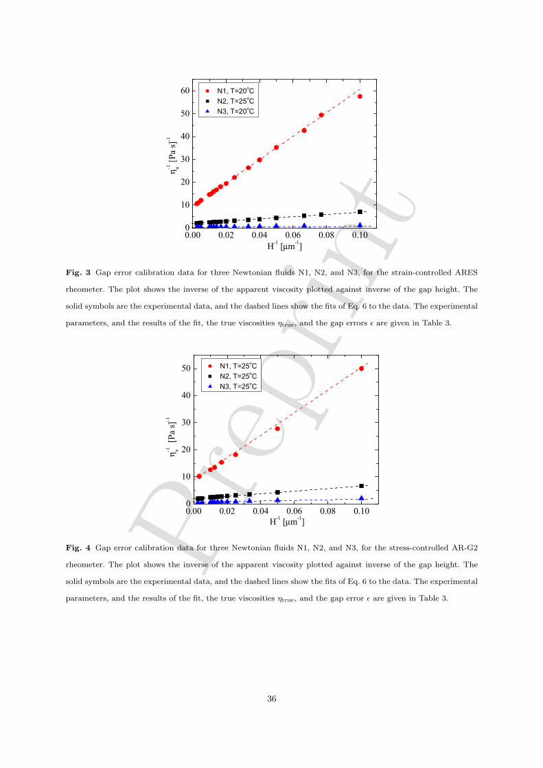
Prep

rint0.00 0.02 0.04 0.06 0.08 0.10

0

10

20

30

40

50

60

!-1 a

[P

a s

]-1

H-1 [µm

-1]

N1, T=20oC

N2, T=25oC

N3, T=20oC

Fig. 3 Gap error calibration data for three Newtonian fluids N1, N2, and N3, for the strain-controlled ARES

rheometer. The plot shows the inverse of the apparent viscosity plotted against inverse of the gap height. The

solid symbols are the experimental data, and the dashed lines show the fits of Eq. 6 to the data. The experimental

parameters, and the results of the fit, the true viscosities ηtrue, and the gap errors ε are given in Table 3.

0.00 0.02 0.04 0.06 0.08 0.100

10

20

30

40

50

!-1 a

[P

a s

]-1

H-1 [µm

-1]

N1, T=25oC

N2, T=25oC

N3, T=25oC

Fig. 4 Gap error calibration data for three Newtonian fluids N1, N2, and N3, for the stress-controlled AR-G2

rheometer. The plot shows the inverse of the apparent viscosity plotted against inverse of the gap height. The

solid symbols are the experimental data, and the dashed lines show the fits of Eq. 6 to the data. The experimental

parameters, and the results of the fit, the true viscosities ηtrue, and the gap error ε are given in Table 3.

36

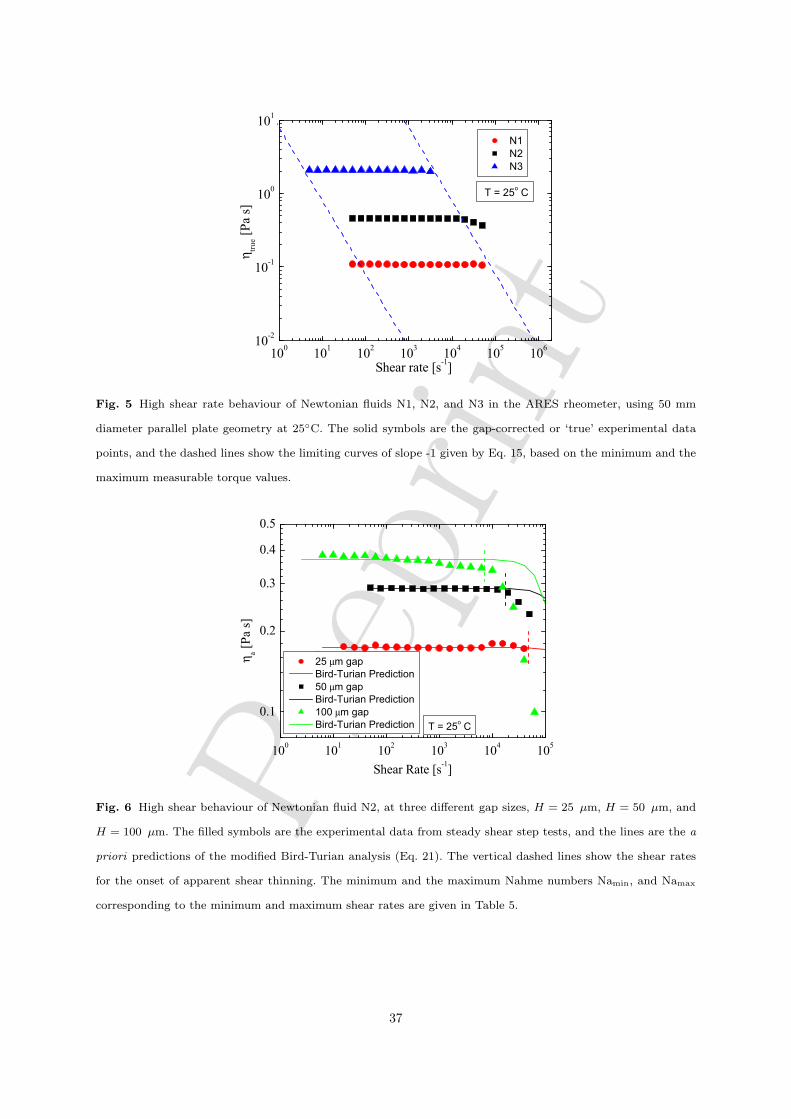
Prep

rint10

-2

10-1

100

101

100

101

102

103

104

105

106

N1

N2

N3

Shear rate [s-1]

!tr

ue [

Pa s

]

T = 25o

C

Fig. 5 High shear rate behaviour of Newtonian fluids N1, N2, and N3 in the ARES rheometer, using 50 mm

diameter parallel plate geometry at 25C. The solid symbols are the gap-corrected or ‘true’ experimental data

points, and the dashed lines show the limiting curves of slope -1 given by Eq. 15, based on the minimum and the

maximum measurable torque values.

100

101

102

103

104

105

0.1

0.2

0.3

0.4

0.5

25 µm gap

Bird-Turian Prediction

50 µm gap

Bird-Turian Prediction

100 µm gap

Bird-Turian Prediction

!a [

Pa s

]

Shear Rate [s-1]

T = 25o C

Fig. 6 High shear behaviour of Newtonian fluid N2, at three different gap sizes, H = 25 µm, H = 50 µm, and

H = 100 µm. The filled symbols are the experimental data from steady shear step tests, and the lines are the a

priori predictions of the modified Bird-Turian analysis (Eq. 21). The vertical dashed lines show the shear rates

for the onset of apparent shear thinning. The minimum and the maximum Nahme numbers Namin, and Namax

corresponding to the minimum and maximum shear rates are given in Table 5.

37

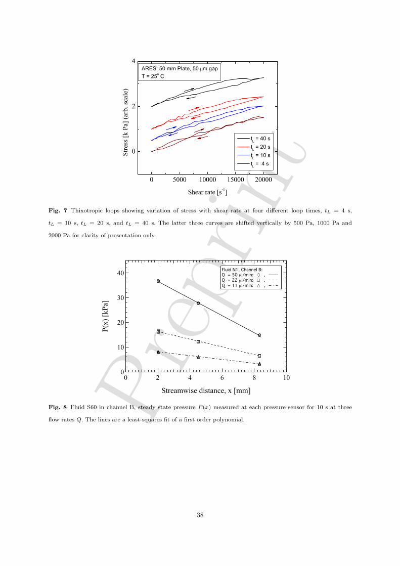
Prep

rint

0 5000 10000 15000 20000

0

2

4

tL = 40 s

tL = 20 s

tL = 10 s

tL = 4 s

Str

ess

[k P

a] (

arb

. sc

ale)

Shear rate [s-1]

ARES: 50 mm Plate, 50 µm gap

T = 25o C

Fig. 7 Thixotropic loops showing variation of stress with shear rate at four different loop times, tL = 4 s,

tL = 10 s, tL = 20 s, and tL = 40 s. The latter three curves are shifted vertically by 500 Pa, 1000 Pa and

2000 Pa for clarity of presentation only.

40

30

20

10

0

P(x)

[kP

a]

1086420

Streamwise distance, x [mm]

Fluid N1, Channel B:Q = 50 µl/min: , Q = 22 µl/min: , Q = 11 µl/min: ,

Fig. 8 Fluid S60 in channel B, steady state pressure P (x) measured at each pressure sensor for 10 s at three

flow rates Q. The lines are a least-squares fit of a first order polynomial.

38

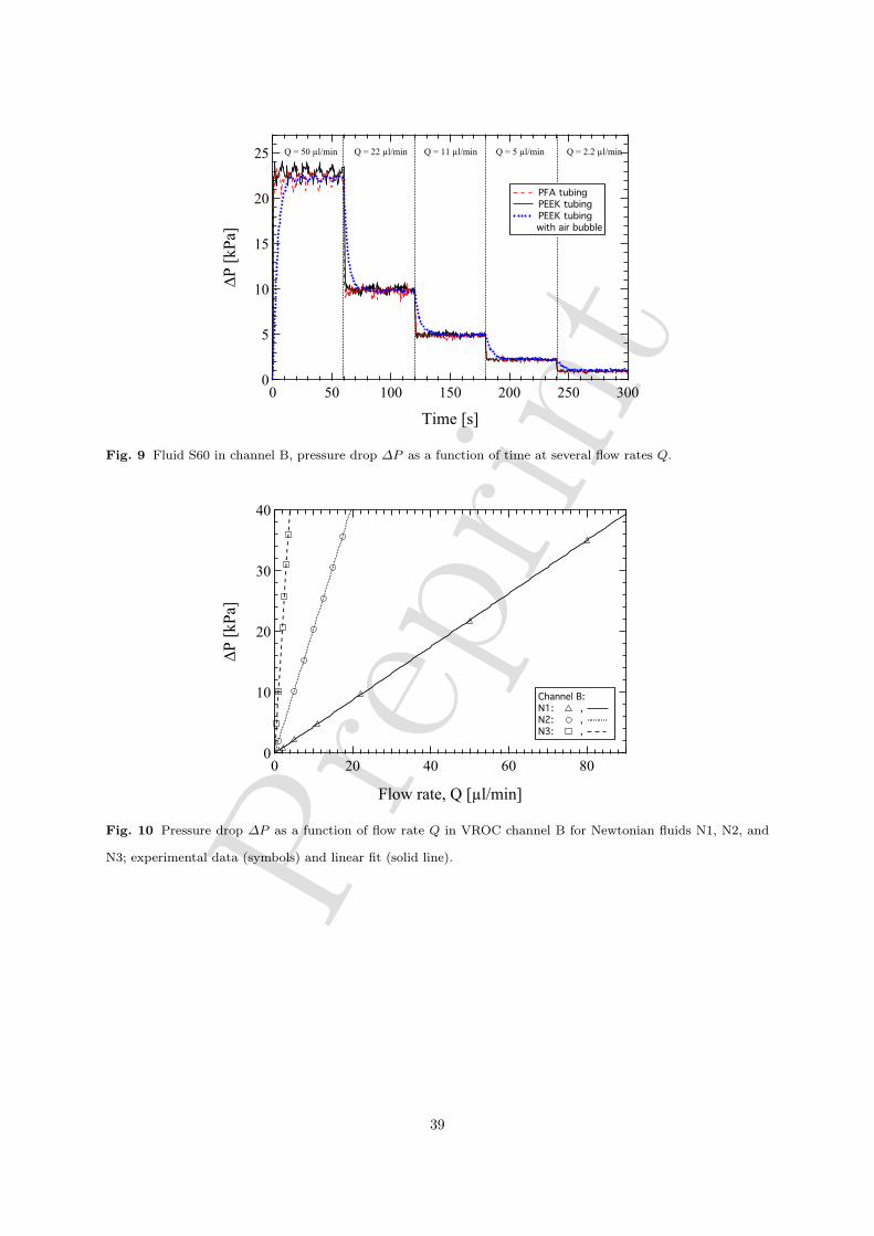
Prep

rint

25

20

15

10

5

0

!P

[kPa

]

300250200150100500

Time [s]

Q = 50 µl/min Q = 22 µl/min Q = 11 µl/min Q = 5 µl/min Q = 2.2 µl/min

PFA tubing PEEK tubing PEEK tubing

with air bubble

Fig. 9 Fluid S60 in channel B, pressure drop ∆P as a function of time at several flow rates Q.

40

30

20

10

0

!P

[kPa

]

806040200

Flow rate, Q [µl/min]

Channel B:N1: , N2: , N3: ,

Fig. 10 Pressure drop ∆P as a function of flow rate Q in VROC channel B for Newtonian fluids N1, N2, and

N3; experimental data (symbols) and linear fit (solid line).

39

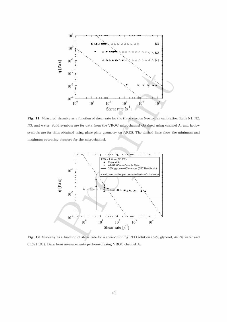
Prep

rint10

-4

10-3

10-2

10-1

100

101

! [

Pa s

]

100

101

102

103

104

105

Shear rate [s-1

]

N3

N2

N1

Fig. 11 Measured viscosity as a function of shear rate for the three viscous Newtonian calibration fluids N1, N2,

N3, and water. Solid symbols are for data from the VROC microchannel obtained using channel A, and hollow

symbols are for data obtained using plate-plate geometry on ARES. The dashed lines show the minimum and

maximum operating pressure for the microchannel.

10-3

10-2

10-1

! [

Pa s

]

100

101

102

103

104

Shear rate [s-1

]

PEO solution (22.5ºC) Channel A AR-G2 60mm Cone & Plate

55% glycerol-45% water (CRC Handbook)

Lower and upper pressure limits of channel A

Fig. 12 Viscosity as a function of shear rate for a shear-thinning PEO solution (55% glycerol, 44.9% water and

0.1% PEO). Data from measurements performed using VROC channel A.

40

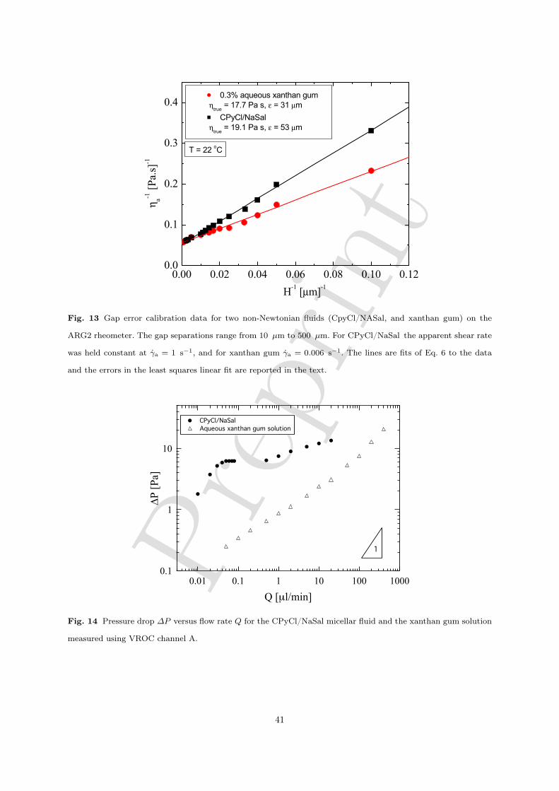
Prep

rint

0.00 0.02 0.04 0.06 0.08 0.10 0.120.0

0.1

0.2

0.3

0.4

H-1 [µm]

-1

0.3% aqueous xanthan gum

!true

= 17.7 Pa s, " = 31 µm

CPyCl/NaSal

!true

= 19.1 Pa s, " = 53 µm

!a

-1 [

Pa.s

]-1T = 22

oC

Fig. 13 Gap error calibration data for two non-Newtonian fluids (CpyCl/NASal, and xanthan gum) on the

ARG2 rheometer. The gap separations range from 10 µm to 500 µm. For CPyCl/NaSal the apparent shear rate

was held constant at γa = 1 s−1, and for xanthan gum γa = 0.006 s−1. The lines are fits of Eq. 6 to the data

and the errors in the least squares linear fit are reported in the text.

0.1

1

10

!P

[Pa]

0.01 0.1 1 10 100 1000

Q [µl/min]

1

CPyCl/NaSal Aqueous xanthan gum solution

Fig. 14 Pressure drop ∆P versus flow rate Q for the CPyCl/NaSal micellar fluid and the xanthan gum solution

measured using VROC channel A.

41

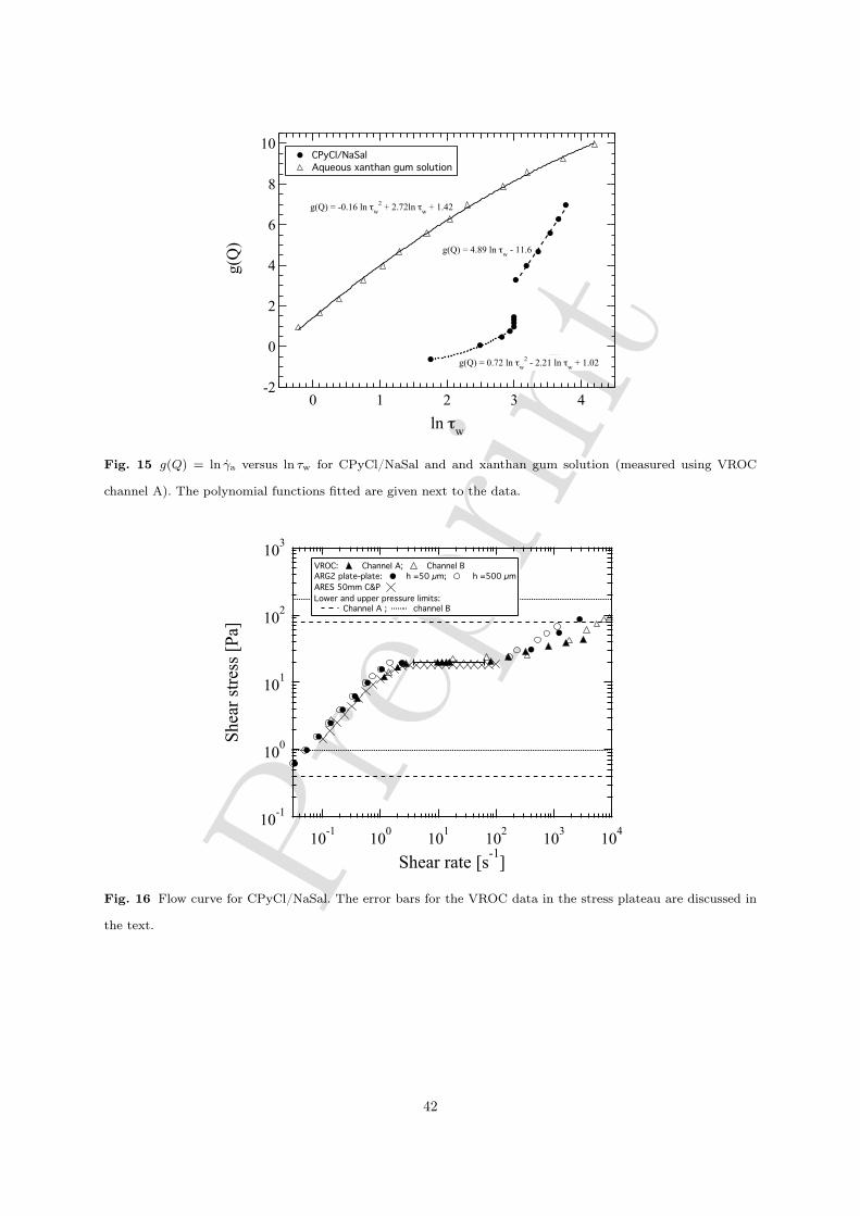
Prep

rint

10

8

6

4

2

0

-2

g(Q

)

43210

ln !w

g(Q) = 0.72 ln !w2 - 2.21 ln !w + 1.02

g(Q) = 4.89 ln !w - 11.6

g(Q) = -0.16 ln !w2 + 2.72ln !w + 1.42

CPyCl/NaSal Aqueous xanthan gum solution

Fig. 15 g(Q) = ln γa versus ln τw for CPyCl/NaSal and and xanthan gum solution (measured using VROC

channel A). The polynomial functions fitted are given next to the data.

10-1

100

101

102

103

Shea

r stre

ss [P

a]

10-1 100 101 102 103 104

Shear rate [s-1]

VROC: Channel A; Channel BARG2 plate-plate: h =50 µm; h =500 µmARES 50mm C&PLower and upper pressure limits: Channel A ; channel B

Fig. 16 Flow curve for CPyCl/NaSal. The error bars for the VROC data in the stress plateau are discussed in

the text.

42

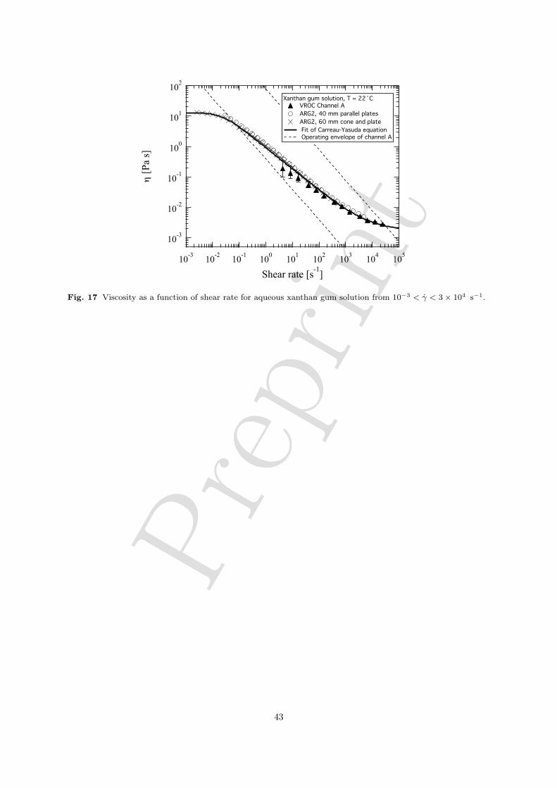
Prep

rint10-3

10-2

10-1

100

101

102

! [P

a s]

10-3 10-2 10-1 100 101 102 103 104 105

Shear rate [s-1]

Xanthan gum solution, T = 22˚C VROC Channel A ARG2, 40 mm parallel plates ARG2, 60 mm cone and plate Fit of Carreau-Yasuda equation Operating envelope of channel A

Fig. 17 Viscosity as a function of shear rate for aqueous xanthan gum solution from 10−3 < γ < 3× 104 s−1.

43

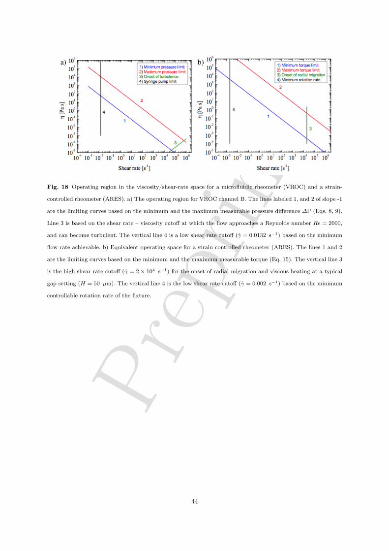
Prep

rint

a) b)

Fig. 18 Operating region in the viscosity/shear-rate space for a microfluidic rheometer (VROC) and a strain-

controlled rheometer (ARES). a) The operating region for VROC channel B. The lines labeled 1, and 2 of slope -1

are the limiting curves based on the minimum and the maximum measurable pressure difference ∆P (Eqs. 8, 9).

Line 3 is based on the shear rate – viscosity cutoff at which the flow approaches a Reynolds number Re = 2000,

and can become turbulent. The vertical line 4 is a low shear rate cutoff (γ = 0.0132 s−1) based on the minimum

flow rate achievable. b) Equivalent operating space for a strain controlled rheometer (ARES). The lines 1 and 2

are the limiting curves based on the minimum and the maximum measurable torque (Eq. 15). The vertical line 3

is the high shear rate cutoff (γ = 2× 104 s−1) for the onset of radial migration and viscous heating at a typical

gap setting (H = 50 µm). The vertical line 4 is the low shear rate cutoff (γ = 0.002 s−1) based on the minimum

controllable rotation rate of the fixture.

44