1

Author version: J. Asian Earth Sci., vol.62; 2013; 616-626 High-resolution residual geoid and gravity anomaly data of the northern Indian Ocean - an input to geological understanding

K.M. Sreejith1*, S. Rajesh3, T.J. Majumdar2, G. Srinivasa Rao4, M. Radhakrishna4, K.S. Krishna5

and A.S. Rajawat1

1 Geosciences Division, Marine, Geo and Planetary Sciences Group, Space Applications Centre (ISRO), Ahmedabad – 380015, India

2Space Applications Centre (ISRO), Ahmedabad – 380015, India 3 Wadia Institute of Himalayan Geology, Dehradun - 248001, India 4 Department of Earth Sciences, Indian Institute of Technology Bombay, Powai, Mumbai - 400076, India 5 CSIR - National Institute of Oceanography, Dona Paula, Goa - 403004, India *Corresponding Author (e-mail: sreejith81@gmail.com)

Abstract

Geoid data are more sensitive to density distributions deep within the Earth, thus the data are useful for studying the internal processes of the Earth leading to formation of geological structures and activities. In this paper, we present much improved version of high resolution (1’×1’) geoid anomaly map of the northern Indian Ocean generated from the altimeter data obtained from Geodetic Missions of GEOSAT and ERS-1 along with ERS-2, TOPEX/POSIDEON and JASON satellites. The geoid map of the Indian Ocean is dominated by a significant low of -106 m south of Sri Lanka, named as the Indian Ocean Geoid Low (IOGL), whose origin is not clearly known yet. The residual geoid data are retrieved from the geoid data by removing the long-wavelength core-mantle density effects using recent spherical harmonic coefficients of Earth Gravity Model 2008 (EGM 2008) up to degree and order 50 from the observed geoid data. The coefficients are smoothly rolled off between degrees 30-70 in order to avoid artifacts related to the sharp truncation at degree 50. With this process we observed significant improvement in the residual geoid data when compared to the previous low-spatial resolution maps (Majumdar and Bhattacharyya, 2004; Majumdar et al., 2006). The previous version was superposed by systematic broad regional highs and lows (like checker board) with amplitude up to ±12 m, though the trends of geoid in general match in both versions. These methodical artifacts in the previous version may have arisen due to the use of old Rapp’s geo-potential model coefficients, as well as sharp truncation of reference model at degree and order 50. Geoid anomalies are converted to free-air gravity anomalies and validated with cross-over corrected ship-borne gravity data of the Arabian Sea and Bay of Bengal. The present satellite derived gravity data matches well with the ship-borne data with Root Mean Square Error (RMSE) of 5.1-7.8 mGal. Spectral analysis of ship-borne and satellite data suggested that the satellite gravity data have a resolution down to 16-18 km. Further, the geoid, residual geoid and gravity anomalies are integrated with seismic data along two profiles in the Bay of Bengal and Arabian Sea, and inferences have been made in terms of density distributions at different depths. The new residual geoid anomaly map shows excellent correlation with regional tectonic features such as Sunda subduction zone, volcanic traces (Chagos-Laccadive, Ninetyeast and 85°E ridges, etc.) and mid-ocean ridge systems (Central Indian and Carlsberg ridges).

Key Words: satellite altimetry, geoid, residual geoid, Indian Ocean

2

1. Introduction

Geoid is the equi-potential surface of gravity which best approximate the mean sea level in the absence of

external gravitational field, and geoid undulations from the reference ellipsoid are called geoid anomalies.

These anomalies can be computed by removing the mean dynamic ocean topography from the time

averaged ocean surface height measurements of satellite altimeter datasets. High spatial and temporal

resolution of the geoid data are achieved by combining the altimeter data obtained from Geodetic and

Exact Repeat missions. While, the geoid models computed directly using GRACE and CHAMP satellites

are accurate only wavelengths >160 km (Tapley and Kim, 2001), the precise measurements (accuracy of

~1 cm at 800 km) of short wavelength variations in the Sea Surface Height (SSH) by the satellite

altimeters allow us to compute the high-resolution geoid.

The geoid data are, in general, dominated by very long-wavelength (>3000 km) anomaly components

contribute by the deep seated sources. In order to study the lithospheric-scale structures, the long-

wavelength core-mantle density effects have to be removed from the geoid data. For this purpose, the

spherical harmonic coefficients of reference geoid models are used. The resulting geoid is then generally

referred as the residual geoid, and the data are sensitive to the anomalous density distributions lie within

the lithosphere generally corresponding to mantle convection processes (McKenzie et al., 1980).

However, care must be taken while removing the long-wavelength reference geoid as it significantly

affects the amplitude and wavelength characteristics of the residual geoid anomalies. Sandwell and

Renkin (1988) cautioned that improper removal of long-wavelength reference geoid can generate regular

pattern of highs and lows in the residual geoid data over the oceanic regions, and highlighted one such

data artifact in the Pacific Ocean which was attributed to the mantle convection processes (McKenzie et

al., 1980)

In this paper, we made an attempt to improve the existing geoid and residual geoid anomaly maps of the

northern Indian Ocean (Majumdar and Bhattacharyya, 2004; Majumdar et al., 2006 hereafter called as

previous maps) by incorporating a refined data reduction procedure that dwells on the enhanced

resolution of recent Earth Gravity Model-2008 (EGM 2008) and adept truncation of model coefficients

for the removal of long-wavelength reference geoid. Thus, the major objectives of the present study are to

1) to present updated high resolution (1’×1’) geoid and residual geoid anomaly maps of the northern

Indian Ocean 2) demonstrate the efficacy of the present maps with the ‘previous maps’ 3) use the geoid

data to generate high-resolution gravity anomalies, and validate them with ship-borne gravity anomalies

4) finally, to carry out a preliminary analysis of these maps together with a comparative study of ship-

track as well as satellite derived free-air gravity anomalies and the residual geoid anomalies along two

regional multi-channel seismic reflection profiles across the Bay of Bengal and Arabian Sea.

3

2. Data and methodology

Geodetic Missions of GEOSAT and ERS-1 along with ERS-2, TOPEX/POSIDEON and JASON

satellites (Andersen and Kundsen, 2009) are utilized for recovery of geoid and gravity data over the

Indian Ocean. The procedure for retrieval of gravity from the altimeter data is briefly explained in Fig.1.

Two types of corrections, i) instrumental and ii) environmental, are necessary for the altimeter range

measurements. The instrument corrections account for the Doppler-shift errors, oscillator-shift errors,

acceleration errors, etc. The sources of instrument errors and their effect on the SSH measurements for

different satellites are described in their respective Geophysical Data Records (GDR). The environmental

corrections accounts for the path-delay in travel time due to water vapor (wet tropospheric correction),

dry gases (dry tropospheric corrections) and electrons in ionosphere (ionospheric correction). Apart from

these atmospheric effects, the returned altimeter is affected by instantaneous effects of the sea surface due

to tidal forces and pressure of specular reflectors, winds and waves. The errors in SSH due to ocean tides

are corrected by interpolating surface tide height obtained from various tidal models along satellite track

(Andersen and Kundsen, 2009). The atmospheric pressure loading (inverse barometric effect) is corrected

using a global mean pressure of 1013 mbar (Andersen and Kundsen, 2009). Re-tracking of the raw

waveforms of GM altimeter data is generally considered to improve the coverage and hence resolution of

the geoid or gravity (Maus et al., 1998; Bansal et al., 2005; Sandwell and Smith, 2008). The mean sea

surface was derived using re-tracked products of GEOSAT and ERS-1 data sets. The ERS-1 GM data

were double re-tracked using the rule-based expert re-tracking system which has significantly enhanced

the number of data, particularly in coastal regions (Andersen et al., 2010) and probably remove the

spurious jumps in ERS-1 profiles as reported earlier (Bansal et al., 2005). The re-tracked GM and mean

EM are corrected for seasonal, orbital and other long-wavelength effects by cross-over adjustments with

minimum variance criteria (Andersen and Kundsen, 2009). The geoid is determined by removing mean

dynamic topography from the time averaged mean sea-surface data. The effect of environmental errors in

SSH measurements and details of the models used for the corrections are different for different satellite

systems. These are discussed in detail in Andersen and Kundsen (2009) and hence not reproduced here.

In the present study, the EGM2008 coefficients (Pavlis et al., 2008) up to degree and order 50 are utilized

to remove the long-wavelength components of the geoid to obtain the residual geoid. As the sharp

truncation of spherical harmonic coefficients at a particular degree would cause side lobes in the spatial

structures of the truncated fields (create artifacts), the EGM 2008 coefficients are smoothly rolled off

between degrees 30-70. The gentle cutting of spherical harmonic coefficients is achieved by smooth

rolling of function f (n) from 1 to 0 between the lower to higher orders. This can be represented as

4

( ) 1224

+⎟⎟⎠

⎞⎜⎜⎝

⎛−−

−⎟⎟⎠

⎞⎜⎜⎝

⎛−−

=ab

a

ab

a

nnnn

nnnnnf

Where na and nb are lower and higher orders (ICGEM, http://icgem.gfz-

potsdam.de/ICGEM/potato/gentlecut_engl.pdf)

The conversion of geoid grid to gravity anomaly is carried out using 2D Fourier transform method

(Haxby et al., 1983). EGM2008 geoid model were removed from the altimeter derived geoid data before

transforming to gravity data. In order to avoid the edge effects, the Fourier transform is applied for

extended area of 1 degree on either side. The full spectrum gravity field is recovered by restoring the

gravity effect of the EGM 2008 geoid field.

3. Results

3.1 High-resolution geoid and residual geoid anomaly maps of the northern Indian Ocean

The resultant geoid anomaly generated after removing mean dynamic components of the mean surface

data is presented in Fig. 2. The geoid map of the Indian Ocean is dominated by the deep geoid low of

about -106 m appearing south of Sri Lanka and is known as the Indian Ocean Geoid Low (IOGL) (Fig.

2). The residual geoid anomaly map of northern Indian Ocean is presented in Fig. 3a. Unlike the geoid

map the residual geoid map correlate well with the regional tectonic features lie within the lithosphere,

and these are discussed in detail in section 4.

Present residual geoid map is compared with that of the previous low-spatial resolution maps of

Majumdar and Bhattacharyya (2004) and Majumdar et al. (2006), and noticed that the authors have used

Rapp’s geo-potential coefficients (Rapp, 1981, 1982) up to degree and order 50 as reference geoid for the

generation of residual geoid data. Following their procedure, Rapp’s geo-potential model truncated at

degree 50 was removed from the present geoid data to generate residual geoid map (Fig. 3b). Though the

trends of geoid anomalies in both versions generally match, the previous version was superposed by

systematic broad regional highs and lows with amplitude up to ±12 m (Figs. 3a and 3b). Apart from the

broad highs and lows, the previous geoid map also differs from the revised map in terms of anomaly

patterns and magnitude. The Broad cusp shaped low in the northern Bay of Bengal region is completely

absent in the new map (Fig. 3a), where the geoid anomalies are trending nearly North-South. Further the

map also brings out a prominent high between the 85°E Ridge and eastern continental margin of India. In

the western Indian Ocean, the Carlsberg and Central Indian ridges, Arabian and Somali basins are clearly

mapped in the revised residual geoid map. In the previous geoid map, these features are masked by broad

high in the Arabian Basin and low in Somali Basin. Comparison of residual geoid fields along the seismic

5

lines MAN-01 and RE-11 also clearly suggests that the present residual geoid data better correlates

matches with the basement structures (see for further details in Section 4.2).

The present study highlights two possible reasons for the difference in the amplitude, wavelength and

anomaly patterns in both old and new versions of residual geoid maps. 1) The new version uses EGM

2008 geoid model instead of old low-resolution Rapp’s model for the removal of deeper earth effects 2)

The new version uses adept bi-harmonic truncation model to cut the spherical harmonic coefficients from

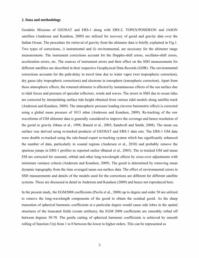
degree 30 to 70, instead of sharp truncation at degree 50. In order to understand these effects, we take the

difference between Rapp’s coefficients truncated sharply at degree 50 and EGM2008 coefficients

smoothly truncated between 30 and 70 (Fig. 4). The difference model grid shows overlapping of low

amplitude short wavelength anomalies as closures in the continuum background of long-wavelength high

amplitude anomalies. The high amplitude anomalies reflects the difference between the EGM2008 and

Rapp’s geoid models, whereas the low-amplitude closures must have caused by the Gibb’s oscillations

introduced as a result of sharp truncation at degree 50.

3.2 Computation of gravity field from the geoid and its validation with ship-borne gravity

Free-air gravity anomaly data derived using the improved geoid and EGM 2008 coefficients are

presented in Fig. 5. For validation purpose, the satellite derived gravity data are compared with ship-

borne gravity profile data, MAN-01 and RE-11 of the Arabian Sea and Bay of Bengal. These areas are

selected because of the availability of reasonably good number of ship-borne gravity profile data. It is

known that ship-borne gravity profile data posses considerable discrepancies at intersecting tracks due to

various reasons; like systematic instrument errors, cross-coupling, loosing reference to an absolute

gravity datum and uncertainties in the navigation system, errors in Eotvos correction, etc. (Wessel and

Watts, 1988). In this study, each ship track data was checked for spikes using statistical reporting of

minimum, maximum, mean and standard deviation and then the outliers were removed. The edited tracks

were further adjusted for cross-over errors using X2SYS package of Wessel (2010). After cross-over

adjustments, the standard deviation of marine gravity data were reduced form 9.5798 mGal to 3.35791

mGal for Arabian Sea and from 13.3068 mGal to 9.9923 mGal for Bay of Bengal.

Satellite derived gravity data are extracted along ship tracks and the error statistics are computed for both

original and corrected ship-borne gravity data (Table 1). The satellite derived gravity data match well

with the cross-over corrected ship-borne data with a RMSE of 5.1188 mGal and 7.7554 mGal for Arabian

Sea and Bay of Bengal, respectively. Further, the coefficient of determination ( 2R ) which explains the

goodness of linear fit between the ship and satellite data were also found to be high (~0.94 for the

Arabian Sea and 0.95 for the Bay of Bengal). When compared to the uncorrected ship-borne data, the

cross-over corrected data matches better with the satellite data with significant improvement in error

6

statistics (Table 1). The along-track difference between ship-borne and satellite data of both Arabian Sea

and Bay of Bengal along with their overall error distribution is presented in Figs. 6a and 6b, respectively.

The histogram plot (Fig. 6b) suggests that for Arabian Sea, about 90% of the satellite data matches with

the ship-borne data within an error limit of ±10 mGal; whereas, for the Bay of Bengal this is about 80%.

We also compare the Sandwell and Smith (2009) satellite gravity, the up-dated version of their ERS-1

marine satellite gravity data (Sandwell and Smith, 1997), and the present satellite gravity data with cross-

over corrected ship-borne data. Both satellite derived gravity data sets were compared over by taking the

standard deviations of their difference grids. These give average standard deviations of 4.2 mGal and 4.5

mGal for both Arabian Sea and Bay of Bengal respectively. Further, Sandwell and Smith data were

compared with the ship-borne data (cross over corrected) and the error statistics are compared to that of

the present gravity data (Table2). The mean error, RMSE and R2 for the present gravity and that of

Sandwell and Smith with the ship-borne data are closely matching. However, it is observed that in

Arabian Sea the present gravity data matches better with the ship-borne data, whereas in Bay of Bengal

the Sandwell and Smith data has better match. Thus, both these analysis suggest that the present gravity

has comparable accuracy to the Sandwell and Smith global gravity data.

To quantify the short-wavelength resolution of the present satellite data we have carried out power

spectrum and spectral coherence analysis between the ship-borne and satellite data of Arabian Sea and

Bay of Bengal. The spectral estimation was carried out along a single satellite and ship- borne profile

constructed from all the available ship tracks for both Arabian Sea and Bay of Bengal separately. Earlier

Bansal and Dimri (1999, 2001) considered short segment profiles in their scaling power spectral

estimations due to non-stationary nature of the spectrum. However, for the spectral comparison of

satellite and ship-borne gravity, the longer profiles are better option than shorter profiles as the former

enables ensemble averaging resulting smoother spectral estimates (Small and Sandwell, 1992). The

coherence values with 95% confidence intervals and power spectrum of ship-borne and satellite gravity

profiles for both Arabian Sea and Bay of Bengal are presented in Fig. 7. For both Arabian Sea and Bay of

Bengal profiles the coherence is very high (>0.75) for wavelengths greater than 20 km and then sharply

decreases at shorter wavelength. The minimum wavelength below which the coherence values are <0.5

(λ0.5) is considered as the resolution limit for the satellite gravity data (Marks, 1996). The present analysis

suggests that Bay of Bengal profiles have slightly higher resolution (λ0.5 = 16 km) compared to the

Arabian Sea Profiles (λ0.5 = 18 km) (Fig. 7). However, it should be noted that the accuracy of the Arabian

Sea profiles are better than that of Bay of Bengal profiles (Table-1). This may be due to the use of longer

profiles for Bay of Bengal, which can lead to spectral averaging over larger distances giving better

resolution. For Arabian Sea and Bay of Bengal profiles the power spectral density of the satellite profile

is comparable to that of ship-borne profiles for λ > 18 and λ > 16 respectively, whereas at lower

7

wavelengths the ship-borne profiles show much higher power (Fig. 7). Thus, both the coherence and

power spectrum analysis suggests that the present gravity field has a resolution of about 18 and 16 km in

the Arabian Sea and Bay of Bengal, respectively.

Further, ship-borne and satellite gravity data are compared from two representative profiles namely RE-

11 and MAN-01 from the Arabian Sea and the Bay of Bengal respectively, as shown in Figs. 8a and 8b.

Comparison reveals that both ship-borne and satellite data are in good agreement with RMSE of 4.67

mGal along profile RE-11 and 3.71 mGal along profile MAN-01.

4. Discussion

4.1 Geological significance of the geoid and residual geoid anomaly maps

The most salient feature in the geoid map of the northern Indian Ocean is the Indian Ocean Geoid Low

(IOGL) which appears as a very long wavelength feature of greater than 15000 km and covers the entire

Indian Ocean. The origin of IOGL is still not clearly understood. Chekunov et al. (1984) suggested that

the IOGL could be due to uncompensated oceanic crust, indicating that the mass anomalies are within the

crust. This theory has not received the acceptance because long-wavelength nature of the IOGL favors

the presence of mass anomalies at much deeper depth. Based on mantle convection studies, Chase (1979)

suggested that the source depth of the anomaly could be about 1200 km depth. Alternatively, Kaula

(1970) and Moberly and Khan (1969) have related the IOGL to lack of asthenospheric return flows or

less viscous asthenospheric flows as a consequence of lithospheric plate movements at spreading ridge or

deep trenches. Subsequently, Negi et al. (1987) argued that IOGL could be due to the depression in the

core-mantle boundary. Rajesh (2009) inferred IOGL as major density void related with middle level

lower mantle flow and computed the source depth at ~1800 km based upon geoid anomaly wavelength

and the degree harmonics. Recently, based on seismic topographic studies Spasojevic et al. (2010)

suggested that about 20% of the IOGL could be attributed to mantle structures shallower than 1000 km.

Further, they opined that IOGL could be related to Tethyan subduction during the Mesozoic period.

Considering these hypotheses and the broad nature of the anomaly, one can infer that the IOGL could be

caused by mass anomalies related to multiple sources. Detailed investigation with multiple wavelength

geoids along with seismic tomography is needed to understand the origin and nature of the IOGL.

It is observed that the geoid data gradually increases from ~-106 m to ~-50 m from the centre of IOGL

(79°E and 5°S) to about 15,000 km radially (Fig. 2). However, towards eastern Indian Ocean the IOGL

trend abruptly ends at 90°E meridian, while the trend gradually extent in the western Indian Ocean up to

60°E longitude. Presence of the Andaman-Sunda subduction zone in the eastern Indian Ocean has

resulted the IOGL trend as high dense north south lineated contours between 85°E to 90°E longitudes.

8

The active subduction zones are in general, characterized by two contrasting geoid anomalies 1) positive

anomaly caused by cold upper mantle slabs and 2) negative anomalies related to dynamic topography

caused by the depression in upper mantle (Hager, 1984). Positive anomalies along Andaman-Sunda

subduction zone suggests that the geoid anomalies are primarily controlled by the mass anomalies caused

by the subduction of cold lithospheric slab. On close observation, it can be inferred that the Andaman

Subduction zone is associated with low geoid values (-55 to -60 m) in comparison to that of the Sunda

region (-30 to -35 m). These variations could be attributed to differences in slab geometry related to

oblique and perpendicular trends of subduction in Andaman and Sunda regions, respectively.

In the western Indian Ocean, the rift-valley of the Carlsberg Ridge is clearly marked in the geoid map as

NW-SE tending snicks in the contour map (Fig. 2). The Owen fracture zone, a tectonic feature connects

the Carlsberg Ridge with the Sheba Ridge and extends further in the northern Arabian Sea, the feature

can be clearly marked in the geoid data. Another prominent feature observed in the geoid map is the

NW–SE trending lineation from 5°S to equator and west of 75°E meridian, probably indicating the trace

of the Vishnu fracture zone. Norton and Slater (1979) opined that Vishnu fracture zone facilitated the

movement of Madagascar away from India at around 85 Ma. The geoid pattern associated with the

Vishnu fracture zone also gives an indication that this fracture zone may have acted as a regional

lithospheric boundary separating the eastern Indian Ocean province from the western Indian Ocean

region. Further studies are required to investigate the role of Vishnu fracture zone in the geodynamical

evolution of the surrounding ocean basins. Apart from the major lithospheric plate boundaries,

continental shelf-slope of the western and eastern margins of India could be identified from the geoid

data.

The new residual geoid anomaly data of the northern Indian Ocean (Fig. 3a) ranges from -7 to 7 m and

are in excellent correlation with regional tectonic features of the region. In eastern Indian Ocean, the

Andaman-Sunda subduction system is marked by strong E-W residual geoid gradients. The trench axis is

associated with geoid low of about -3.5 m with positive geoid anomalies towards west. The Ninetyeast

Ridge (NER) is associated with positive geoid anomalies and the trend of the ridge could be clearly

marked up to 7°N. North of 7°N, isolated highs associated with NER topography appears to merge with

the broad positive geoid highs oriented along the subduction arch. The 85°E Ridge is marked with

negative residual geoid anomalies towards north of 5°N and positive anomaly in south as noticed earlier

by Krishna et al.(2009). The NW-SE trending Comorin Ridge is also observed in the residual geoid data.

The northern portion of the ridge is associated with about 0.5 m anomaly, whereas the southern portion of

the ridge is associated with greater than 2 m anomaly. The contrasting anomalies could be related to the

emplacement of the ridge material on rifted continental crust in north and oceanic crust with underplated

9

material in south portion of the ridge (Sreejith et al., 2008). Major off-shore sedimentary basins such as

Krishna-Godavari, Cauvery and Mannar basins are clearly marked with broad negative residual geoid

contours.

In western Indian Ocean, the Carlsberg and Central Indian ridges are associated with geoid highs with a

clear low marking the ridge rift-valley. The Laxmi Ridge and Chagos-Laccadive ridges are also

associated with negative and positive geoid anomalies, respectively. Further the data can be utilized to

demarcate the extent of Owen Fracture Zone as NE-SW tending negative geoid anomalies.

4.2 Comparative analysis of geoid and gravity data with seismic data

The revised geoid, residual geoid and gravity data of the northern Indian Ocean are correlated with deep

seismic reflection data along two profiles: MAN-01 and RE-11 to examine the basement structural

features and their mass distributions within the crust (Figs. 8a and 8b).

Basement topography and the overlying sediment units interpreted from seismic reflection profile (MAN-

01) along 14.64°N latitude is shown in Fig. 8a (Krishna et al., 2009). The basement in the Bay of Bengal

generally consists of two major aseismic ridges, the 85°E Ridge and Ninetyeast Ridge. The basements

between the shelf edge of the Eastern Continental Margin of India and the 85°E Ridge, and that between

85°ERidge and the Ninetyeast Ridge form the Western and Central basins, respectively. Based on seismic

results of the Bay of Bengal, Curray et al. (1982), Gopala Rao et al. (1997) and Michael and Krishna

(2011) have divided the entire sediment section into two sedimentary packages and interpreted that the

lower package was deposited mainly from the rivers of peninsular India, whereas the upper package was

deposited by the discharges of Ganges and Brahmmaputra rivers after establishing the contact of the

Indian subcontinent with the Asian continent. Further the packages are classified as pre- and post-

collision sediments and are separated by an erosional-type unconformity developed in Paleocene age

(Fig. 8a) (Moore et al., 1974). The pre-collision sediment package consists of pelagic and terrigeneous

sediments deposited prior to the India-Eurasia collision, whereas, the post-collision part mostly consists

of Bengal Fan sediments. The 85°E Ridge acts as a structural boundary for dividing the thick Bengal Fan

sediments into Western and Central basins (Curray et al., 1982).

The free-air gravity data along the profile MAN-01 (Fig. 8a) closely follow the basement structure

suggesting that most part of the anomaly was contributed by the basement-sediment density contrast. The

residual geoid data also follow the trend of the free-air anomaly, but appears to be much smooth and

indicate its lesser sensitivity to the basement-sediment density contrast. Residual geoid could be a better

choice than free-air gravity data for modeling and interpretation of crustal structure and Moho

configurations. The 85°E Ridge and Ninetyeast Ridge topography are associated with negative and

10

positive residual geoid/gravity anomalies, respectively. However, geoid data are devoid of any signatures

as they are related with deep crust/mantle mass anomalies. Steep gradients in the geoid data towards the

continental margin indicate westward tilt of lithosphere associated with progressive aging towards west.

Geoid, residual geoid and gravity data are extracted along the seismic profile RE-11 of the western

continental margin of India and stacked the data with the interpreted seismic results (Fig. 8b). Seismic

reflection results depict two major structural rises, the Panikkar Ridge and the Laxmi Ridge. The Laxmi

Basin has smooth topography with three isolated seamounts: Wadia, Panikkar, and Raman in the central

part (Krishna et al., 2006). The Laxmi Ridge is associated with a prominent gravity and residual geoid

low, whereas the Panikkar Ridge has high anomaly. A regional shift in gravity, residual geoid and geoid

data is clearly observed on east of the Laxmi Ridge (Fig. 8b). Earlier, based on seismic and geophysical

model studies Krishna et al. (2006) marked the Ocean-Continent Boundary on western edge of the Laxmi

Ridge (Fig. 8b).

The present residual geoid data better demarcate basement tectonic features than the previous residual

geoid (Figures 8a and 8b). For example, the Panikkar Ridge along RE-11 is clearly demarcated as local

high in the present residual geoid data whereas this feature is completely absent in the previous residual

geoid. Similarly, the 85° E Ridge along MAN-01 is better demarcated with a regional geoid low in the

present residual geoid when compared with the previous residual geoid.

4. Conclusions

The major conclusions of the present work are as follows

1) Revised high-resolution (1’×1’) geoid, residual geoid and gravity anomaly maps of the northern

Indian Ocean were prepared using satellite altimeter data and high-resolution harmonic coefficients

of recent Earth Gravity Model 2008 (EGM 2008).

2) The geoid map of the Indian Ocean is dominated by a significant low of -106 m at the south of Sri

Lanka, named as the Indian Ocean Geoid Low (IOGL), which is believed to be originated from the

source lying at deeper depths. In contrast, the Andaman-Sunda Subduction Zone is associated with

prominent geoid highs. Further, it is inferred that the geoid values (55-60 m) of the Andaman

Subduction zone is comparatively low to the Sunda region (30-35 m). These differences in geoid

heights could be attributed to differences in slab geometry related to oblique and perpendicular

trends of subduction for Andaman and Sunda regions, respectively.

3) The revised residual geoid data were compared with the previous version maps. Although the

trends of geoid anomalies in both versions generally match, the previous version have perceptive

11

difference in anomaly magnitude and pattern with broad regional highs and lows up to ±12 m. Our

comparative study highlights two possible reasons that augmented into new geoid and residual

geoid of northern Indian Ocean, they are 1) The new version uses EGM 2008 geoid model rather

than old low resolution Rapp’s model for the removal of deeper earth effects 2) The new version

used adept bi-harmonic truncation model to cut the spherical harmonic coefficients from degree 30

to 70, instead of sharp truncation at degree 50. The old Rapp’s model might have caused the broad

highs and lows and isolated lobs due to sharp truncation at degree 50. The new residual geoid

anomaly map shows excellent correlation with regional tectonic features such as Sunda subduction

zone, volcanic traces (Chagos-Laccadive, Ninetyeast and 85°E ridges etc.) and mid-ocean ridge

systems (Central Indian and Carlsberg ridges).

4) Geoid anomalies are converted to free-air gravity anomalies and validated with ship-borne gravity

data from Arabian Sea and Bay of Bengal. The present satellite derived gravity data match well

with the ship-borne data with RMSE of about 5.1 to 7.8 mGal. Spectral analysis of ship-borne and

satellite data suggested that the satellite gravity has a resolution of about 16-18 km.

5) Geoid, residual geoid and gravity anomalies are integrated with seismic reflection data

interpretations along two profiles in the Bay of Bengal and Arabian Sea. The analysis suggest that

the residual geoid data are more sensitive to the deeper crust/mantle mass anomalies and could be

effectively use for the modeling of crust and upper mantle structures.

Acknowledgments

A. S. Kirankumar, Director-SAC, A. K. Gupta, Director-WIHG, S.R. Shetye, Director-NIO, J.S.

Parihar, DD, EPSA, and Ajai, GD, MPSG have encouraged the joint studies. TJM thanks CSIR, New

Delhi for Emeritus Scientist Fellowship since January 2011. Figures were prepared using GMT

software of Wessel and Smith (1998). This work is carried out jointly by SAC, WIHG, IIT-B and NIO

as a part of SARAL/AltiKa and MOP II – Marine Lithospheric Studies program of SAC-ISRO. This is

NIO contribution numer:

References Andersen, O.B., Kunudsen, P., 2009. DNSC08 mean sea surface and mean dynamic topography models.

Journal of Geophysical Research 114, C11001, doi: 10.1029/2008JC005179.

Bansal, A. R., Fairhead, J.D., Green C., Fletcher, K.M.U., 2005. Revised gravity for offshore India and the isostatic compensation of submarine features. Tectonophysics, 404, 1-22.

Bansal, A. R., Dimri, V. P., 2001. Depth estimation from the scaling power spectral density of nonstationary gravity profile, Pure and Applied Geophysics 158, 799-812.

12

Bansal, A. R., Dimri, V.P., 1999. Gravity evidence for mid crustal domal structure below Delhi fold belt and Bhilwara super group of western India. Geophysical Research Letters 26(18), 2793-2795.

Chase, C.G, 1979. Subduction, the geoid and lower mantle convection. Nature 282, 464-468.

Chekunov, A.V., Sollugub, V.B., Starostenko, V., Kharetchiko, G.E., Rusakov, V.G., Kosttukovich, A.S., 1984. Strucutre of th earth’s crust and upper mantle below Hindustan and the northern part of the Indian Ocean from geophysical data. Tectonophysics 101, 63-73.

Curray, J.R., Emmel, F.J., Moore, D.G., Russel, W.R., 1982. Structure, tectonics, and geological history of the northeastern Indian Ocean, In: Nairn A.E., Stheli, F.G. (Eds.), The Ocean Basins and Margins-The Indian Ocean. Plenum, New York, 6, pp. 399-450.

Gopala Rao, D., Krishna, K.S., Sar, D., 1997. Crustal evolution and sedimentation history of the Bay of Bengal since the Cretaceous. Journal of Geophysical Research 102, 17747-17768.

Hager, B. H. 1984. Subducted slabs and the Geoid: Constraints on mantle rheology and flow. Journal of Geophysical Research, 89, 6003-6015.

Haxby, F., Karner, G. D., La Brecque, J. L. and Weissel, J. K., 1983. Diggital images of combained oceanic and continental data sets and their use intectonic studies. EOS Transactions American Geophysical Union 64, 995–1004.

ICGEM, Low Pass Filtering of Gravity Field Models by Gently Cutting the Spherical Harmonic Coefficients of Higher Degrees, http://icgem.gfz-potsdam.de/ICGEM/potato/gentlecut_engl.pdf

Kaula, W.H., 1970. Earth’s gravity field. Resolution to global tectonics. Science 169, 982-985.

Krishna, K.S., Gopala Rao, D., Sar, D., 2006. Nature of the crust in the Laxmi Basin (14°-20°N) western continental margin of India. Tectonics 25, TC1006, doi: 10.1029/ 2004TC001747.

Krishna, K.S., Michael, L., Bhattacharyya, R., Majumdar, T.J., 2009. Geoid and gravity anomaly data of conjugate regions of Bay of Bengal and Enderby Basin: New constraints on breakup and early spreading history between India and Antarctica. Journal of Geophysical Research 114, B03102 doi: 10.1029/2008JB005808.

Majumdar, T. J., Bhattacharyya, R., 2004. An atlas of very high resolution satellite geoid/gravity over the Indian offshore, SAC Technical Report SAC/RESIPA/MWRG/ESHD/TR-21/2004, 46 pp., Space Appl. Cent., Ahmedabad.

Majumdar, T. J., Krishna, K. S., Chatterjee, S. Bhattacharyya, R., Michael, L., 2006. Study of high-resolution satellite geoid and gravity anomaly data over the Bay of Bengal. Current Science 90, 211 –219.

Marks, K.M., 1996. Resolution of the Scrpps/NOAA marine gravity field from satellite altimetry. Geophysical Research Letters 23, 2069-2072.

Maus, C., Green, C.M., Fairhead, J.D., I.M., 1998. Improoved Ocean geoid resolution from re6tracked ERS-1 satellite altimeter waveforms. Geophysical Journal International 134, 243-253.

McKenzie, D.P., Watts, A.B., Parsons, B.E., Roufosse, M., 1980. Platform of mantle convection beneath Pacific Ocean, Nature 288, 442-446.

Michael, L., K.S. Krishna, Dating of the 85°E Ridge (northeastern Indian Ocean) using marine magnetic anomalies, Current Science 100, 1314-1322, 2011.

Moberly, R., Khan, N.A., 1969. Interpretation of the sources of satellite determined gravity field. Nature 223, 263-267.

13

Moore, D.G., Curray, J.R. Raitt, R.W., Emmel, F.J., 1974. Stratigraphic-seismic section corrrlations and implications to Bengal Fan history. Initial Report; Deep Sea Drilling Project 22 403-412.

Negi, J.G, Thakur, N.K., Agarwal, P.K., 1987. Can depression of the core-mantle interface causes coincident Magsat and Geoidal ‘lows’ of the central Indian Ocean. Physics of Earth and Planetary Interiors 45, 68-74.

Norton, I.O., Sclater, J.G., 1979. A model for the evolution of the Indian Ocean and the breakup of Gondwanaland. Journal of Geophysical Research 84, 6803–6830.

Pavlis, N., Holmes, S., Kenyon, S., Factor, J.K, 2008. An Earth gravitational model to degree 2160, Geophysical Research Abstract 10, EGU2008-A-01891.

Rajesh S, 2009. Geoid and the regional density anomaly field in the Indian Plate. Himalayan Geology 30(2), 187-192.

Rapp, R. H., 1981. The earth’s gravity field up to degree and order 180 using Seasat altimeter data, terrestrial gravity data, and other data. Report No. 332, Department of Geodetic Science and Surveying, The Ohio State University, Colombus, Ohio, 53p.

Rapp, R. H., 1982. A FORTRAN program for the computation of gravimetric quantities from high degree spherical harmonic expansions, Report No. 334, The Ohio State University, Department of Geodetic Science and Surveying, Columbus, Ohio, 22p.

Sandwell D.T., Renkin, M.L., 1988. Compensation of Swells and Plateaous in the North Pacific: No direct evidence for Mantle convection. Journal of Geophysical Research 93, 2775-2783.

Sandwell, D. T., W. H. F., Smith 1997. Marine gravity anomaly from Geosat and ERS-1 satellite altimetry, Journal of Geophysical Research 102, 10,039 -10,054, doi:10.1029/96JB03223.

Sandwell, D. T., W. H. F. Smith 2009. Global marine gravity from retracked Geosat and ERS-1 altimetry: Ridge segmentation versus spreading rate. Journal of Geophysical Research 114, B01411, doi:10.1029/2008JB006008.

Small, C., Sandwell, D.T., 1992. A comparison of satellite and ship borne gravity measurments in the Gulf of Mexico. Geophysics 57, 885-893.

Spasojevic, S, Gurnis, M, Sutherland, R. 2010. Mantle upwellings above slab graveyards linked to the global geoid lows. Nature Geoscience 3, doi: 10.1038/NGEO855

Sreejith, K.M., Krishna K.S., Bansal, A.R., 2008. Strucutre and isostatic compensation of the Comorin Ridge, North-Central Indian Ocean. Geophysical Journal International 175, 729–741

Tapley, B.D., Kim, M.C., 2001. Applications to geodesy. In. Fu, L.L., Cazenave (Eds.), Satellite Altimetry and Earth Sciences, Int. Geophys. Ser., Vol. 69. Academic Press, New York, pp. 371-403.

Wessel, P, 2010. Tools for analyzing intersecting tracks: The x2sys package. Computers & Geosciences 36, 348–354.

Wessel, P., Smith, W.H.F., 1998. New, improved version of generic mapping tools released. Eos Transactions, AGU (American Geophysical Union) 79 (47), 579.

Wessel, P., Watts, A.B., 1988. On the accuracy of marine gravity measurements. Journal of Geophysical Research 93, 393–413.

14

List of Tables

Table-1 Comparison of Error statistics of ship borne and satellite marine gravity from the Arabian Sea and Bay of Bengal. Note the differences in RMSE, STDV and 2R after applying cross-over corrections to the ship borne gravity data

Table-2 Table 2 Error statistics for the comparison of cross over corrected ship-bone gravity with satellite gravity (the present study and Sandwell and Smith (2009))

List of Figures

Figure 1 Processing steps involved in Marine geoid and gravity retrieval from the satellite altimeter data

Figure 2 Geoid data of the Northern Indian Ocean. CIR, Central Indian Ridge; CBR, Carlsberg Ridge; LR, Laxmi Ridge; OFZ, Owen Fracture Zone; ASZ, Andaman Subduction Zone; VFZ, Vishnu Fracture Zone. Plate boundaries are marked with red solid line. Solid dashed black line indicates the trends of LR and VFZ.

Figure 3a Residual geoid data calculated by subtracting EGM 2008 spherical harmonic coefficients smoothly truncated between degrees 30 to 70 from the observed geoid. NER, Ninetyeast Ridge; CR, Comorin Ridge; CLR, Chagos Laccadive Ridge

Figure 3b Residual geoid data calculated by subtracting Rapp’s spherical harmonic coefficients up to degree and order 50 from the observed geoid.

Figure 4 Difference between Rapp’s geopotential model up to degree and order 50 and EGM 2008 model smoothly truncated from degree 30 to 70

Figure 5 Free-air gravity anomaly of Northern Indian Ocean. Three Subsets of gravity data from various tectonic domains - A (Continental Margin), B (Central Indian Ridge), C (Ninetyeast Ridge) are shown separately. Positions of seismic profiles MAN01 and RE-11 are also shown.

Figure 6a Along track difference between ship borne and satellite gravity observations of Arabian Sea (AS) and Bay of Bengal (BOB)

Figure 6b Histogram of the difference between ship and satellite gravity along the tracks in Arabian Sea and Bay of Bengal

Figure 7 Coherence and power spectrum (or PSD ?) estimated for ship borne and satellite gravity data of Arabian Sea and Bay of Bengal.

Figure 8a Comparison of geoid, residual geoid and gravity anomalies with seismic data along profile MAN01 in Bay of Bengal (Fig. 5). Satellite gravity is also plotted with the ship borne gravity for comparison

Figure 8b Same as for Fig. 8a for profile RE-11 in Arabian Sea (Fig. 5).

15

Table 1 Error statistics for shipboard and satellite marine gravity comparisons from Arabian Sea and Bay of Bengal. Note the differences in RMSE, STDV and 2R after applying cross-over corrections to the shipboard gravity data.

Table 2 Error statistics for comparison of cross over corrected ship-bone gravity with satellite gravity (the present study and Sandwell and Smith, 2009)

Parameter Arabian Sea Bay of Bengal Present gravity

Sandwell and Smith

(2009)

Present gravity

Sandwell and Smith

(2009) Mean error -1.2983

-5.5122

5.824

1.1319

RMSE 5.1188 6.583 7.7554 5.298

2R 0.9379 0.9386 0.9553 0.9571

Arabian Sea Bay of Bengal No of observations

21,500 23,711

Parameter Cross-over Corrected

Uncorrected Cross-over Corrected

Uncorrected

RMSE 5.1188 6.6145 7.7554 10.1173 STDV 4.9512 6.4462 5.1208 7.2068

2R 0.9379 0.8847 0.9553 0.9204

16

Figure 1

17

Figure 2

18

Figure 3a

Figure 3b

19

Figure 4

20

Figure 5

21

Figure 6a

22

Figure 6b

23

Figure 7

24

Figure 8a

25

Figure 8b