High-resolution imaging through strong atmospheric turbulence and over wide fields-of-view

Stuart M. Jefferies, Douglas A. Hope

Institute for Astronomy, University of Hawaii, 34 Ohia Ku Street, Pukalani, HI, USA 96768 Michael Hart

Steward Observatory, University of Arizona, 933 N. Cherry Ave., Tucson, AZ, USA 85721 James Nagy

Department of Mathematics and Computer Science, Emory University, Atlanta, GA, USA 30322

ABSTRACT We use numerical simulations to study the prospective performance of a dual channel imaging system for observing space-based targets through strong atmospheric turbulence: one channel of the system employs aperture diversity and the other an imaging Shack-Hartmann wave-front sensor. The raw images acquired by this setup are processed using a blind restoration algorithm that captures the inherent temporal correlations in the observed phases. This approach, which strengthens the synergy between the image acquisition and post-processing steps, shows strong potential for providing high-resolution imagery at high levels of atmospheric turbulence. The approach may also allow for the separation of the phase perturbations from different layers of the atmosphere and offers promise for accurate restoration of images with fields of view substantially larger than the isoplanatic angle.

1. INTRODUCTION

The Air Force’s 3-meter class AEOS and Starfire telescopes in Hawaii and New Mexico, respectively, play an important role in monitoring the near space environment for space situational awareness (SSA). Unfortunately, the amount of sky over which images of space objects can be obtained with diffraction-limited resolution is limited to regions where the atmospheric turbulence is benign to moderate (i.e. D/r0 ≤ 15, where D is the diameter of the telescope aperture and r0 is the spatial coherence length of the atmosphere): the resolution of the recovered imagery for the rest of the sky degrades as the depth of atmosphere between the telescope and target increases (and r0 decreases). This means that the quality of the imagery obtained at low elevation angles (i.e. near the horizon) is nearly always inferior to that obtained at high elevation angles.

Motivated by this limitation we investigate an observing/image processing strategy for strong turbulence conditions that offers the potential to both expand the range of elevation angles over which we can obtain high-fidelity imagery, and the fields-of-view that can be accommodated.

2. PROPOSED METHODOLOGY

High-resolution imaging with the AEOS and Starfire telescopes is typically achieved using the full (unpartitioned) aperture and AO compensation. As AO compensation is never 100% effective, the image quality is then further improved through numerical post processing of the data (e.g., using multi-frame blind deconvolution, MFBD [1,2]). For single aperture data this combination of AO compensation and numerical processing can provide diffraction-limited resolution imagery for observations with D/r0 ≤ 15. At higher levels of turbulence the efficiency of the AO compensation deteriorates and increasing reliance is placed on the numerical processing to provide the desired image resolution. However, the efficiency of the numerical processing also deteriorates with increasing turbulence strength and by D/r0~30-40, a level that can be expected for observations acquired at low-elevation angles, even the combination of AO and numerical processing provides little improvement in image quality.

In the above approach to high-resolution imaging, the data acquisition and processing steps are essentially independent of each other. To deal with imagery obtained through strong turbulence (D/r0 ≥ 30) we take a different approach, one that improves the synergy between the image acquisition and processing steps.

Our proposed methodology is based on four observations.

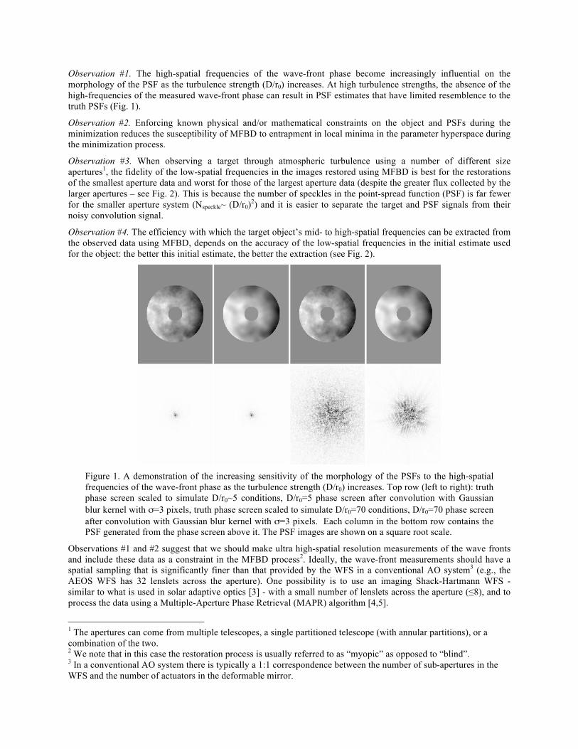
Observation #1. The high-spatial frequencies of the wave-front phase become increasingly influential on the morphology of the PSF as the turbulence strength (D/r0) increases. At high turbulence strengths, the absence of the high-frequencies of the measured wave-front phase can result in PSF estimates that have limited resemblence to the truth PSFs (Fig. 1).

Observation #2. Enforcing known physical and/or mathematical constraints on the object and PSFs during the minimization reduces the susceptibility of MFBD to entrapment in local minima in the parameter hyperspace during the minimization process.

Observation #3. When observing a target through atmospheric turbulence using a number of different size apertures1, the fidelity of the low-spatial frequencies in the images restored using MFBD is best for the restorations of the smallest aperture data and worst for those of the largest aperture data (despite the greater flux collected by the larger apertures – see Fig. 2). This is because the number of speckles in the point-spread function (PSF) is far fewer for the smaller aperture system (Nspeckle~ (D/r0)2) and it is easier to separate the target and PSF signals from their noisy convolution signal.

Observation #4. The efficiency with which the target object’s mid- to high-spatial frequencies can be extracted from the observed data using MFBD, depends on the accuracy of the low-spatial frequencies in the initial estimate used for the object: the better this initial estimate, the better the extraction (see Fig. 2).

Figure 1. A demonstration of the increasing sensitivity of the morphology of the PSFs to the high-spatial frequencies of the wave-front phase as the turbulence strength (D/r0) increases. Top row (left to right): truth phase screen scaled to simulate D/r0~5 conditions, D/r0=5 phase screen after convolution with Gaussian blur kernel with σ=3 pixels, truth phase screen scaled to simulate D/r0=70 conditions, D/r0=70 phase screen after convolution with Gaussian blur kernel with σ=3 pixels. Each column in the bottom row contains the PSF generated from the phase screen above it. The PSF images are shown on a square root scale.

Observations #1 and #2 suggest that we should make ultra high-spatial resolution measurements of the wave fronts and include these data as a constraint in the MFBD process2. Ideally, the wave-front measurements should have a spatial sampling that is significantly finer than that provided by the WFS in a conventional AO system3 (e.g., the AEOS WFS has 32 lenslets across the aperture). One possibility is to use an imaging Shack-Hartmann WFS - similar to what is used in solar adaptive optics [3] - with a small number of lenslets across the aperture (≤8), and to process the data using a Multiple-Aperture Phase Retrieval (MAPR) algorithm [4,5].

1 The apertures can come from multiple telescopes, a single partitioned telescope (with annular partitions), or a combination of the two. 2 We note that in this case the restoration process is usually referred to as “myopic” as opposed to “blind”. 3 In a conventional AO system there is typically a 1:1 correspondence between the number of sub-apertures in the WFS and the number of actuators in the deformable mirror.

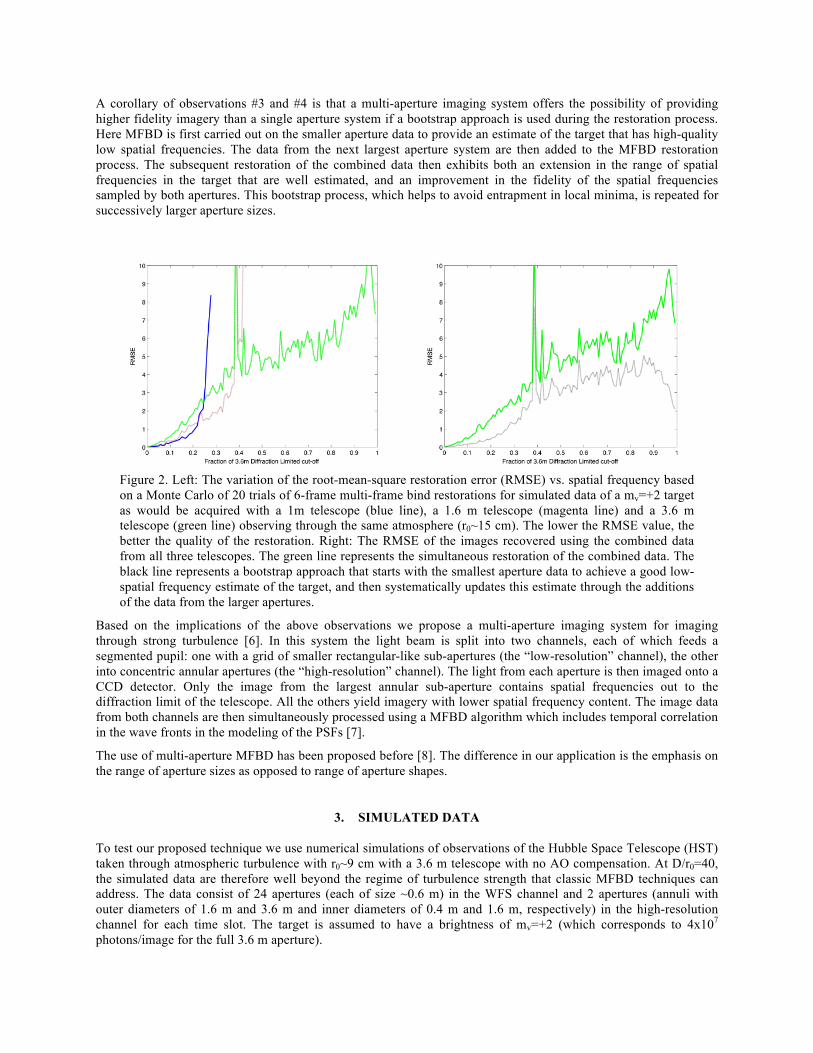
A corollary of observations #3 and #4 is that a multi-aperture imaging system offers the possibility of providing higher fidelity imagery than a single aperture system if a bootstrap approach is used during the restoration process. Here MFBD is first carried out on the smaller aperture data to provide an estimate of the target that has high-quality low spatial frequencies. The data from the next largest aperture system are then added to the MFBD restoration process. The subsequent restoration of the combined data then exhibits both an extension in the range of spatial frequencies in the target that are well estimated, and an improvement in the fidelity of the spatial frequencies sampled by both apertures. This bootstrap process, which helps to avoid entrapment in local minima, is repeated for successively larger aperture sizes.

Figure 2. Left: The variation of the root-mean-square restoration error (RMSE) vs. spatial frequency based on a Monte Carlo of 20 trials of 6-frame multi-frame bind restorations for simulated data of a mv=+2 target as would be acquired with a 1m telescope (blue line), a 1.6 m telescope (magenta line) and a 3.6 m telescope (green line) observing through the same atmosphere (r0~15 cm). The lower the RMSE value, the better the quality of the restoration. Right: The RMSE of the images recovered using the combined data from all three telescopes. The green line represents the simultaneous restoration of the combined data. The black line represents a bootstrap approach that starts with the smallest aperture data to achieve a good low-spatial frequency estimate of the target, and then systematically updates this estimate through the additions of the data from the larger apertures.

Based on the implications of the above observations we propose a multi-aperture imaging system for imaging through strong turbulence [6]. In this system the light beam is split into two channels, each of which feeds a segmented pupil: one with a grid of smaller rectangular-like sub-apertures (the “low-resolution” channel), the other into concentric annular apertures (the “high-resolution” channel). The light from each aperture is then imaged onto a CCD detector. Only the image from the largest annular sub-aperture contains spatial frequencies out to the diffraction limit of the telescope. All the others yield imagery with lower spatial frequency content. The image data from both channels are then simultaneously processed using a MFBD algorithm which includes temporal correlation in the wave fronts in the modeling of the PSFs [7].

The use of multi-aperture MFBD has been proposed before [8]. The difference in our application is the emphasis on the range of aperture sizes as opposed to range of aperture shapes.

3. SIMULATED DATA

To test our proposed technique we use numerical simulations of observations of the Hubble Space Telescope (HST) taken through atmospheric turbulence with r0~9 cm with a 3.6 m telescope with no AO compensation. At D/r0=40, the simulated data are therefore well beyond the regime of turbulence strength that classic MFBD techniques can address. The data consist of 24 apertures (each of size ~0.6 m) in the WFS channel and 2 apertures (annuli with outer diameters of 1.6 m and 3.6 m and inner diameters of 0.4 m and 1.6 m, respectively) in the high-resolution channel for each time slot. The target is assumed to have a brightness of mv=+2 (which corresponds to 4x107 photons/image for the full 3.6 m aperture).

We use a two-layer, frozen flow description of the atmosphere and a Kolmogorov model to generate wave fronts for the different apertures. The wind velocity vectors are commensurate with values observed at Mt Haleakala (~5 m/s for the lower layer and ~ 30 m/s for the upper layer). The point-spread functions (PSFs) corresponding to the wave fronts observed in the different pupils are convolved with a numerical model of the HST to provide noise-free models of the observed images. Poisson noise is then added to these images to simulate the observed data (the imaging cameras are assumed to have negligible read noise: e.g., EMCCDs).

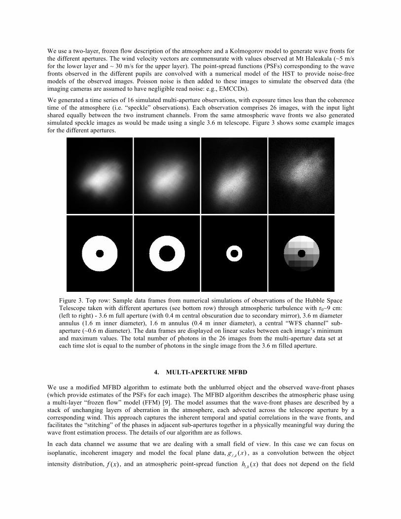
We generated a time series of 16 simulated multi-aperture observations, with exposure times less than the coherence time of the atmosphere (i.e. “speckle” observations). Each observation comprises 26 images, with the input light shared equally between the two instrument channels. From the same atmospheric wave fronts we also generated simulated speckle images as would be made using a single 3.6 m telescope. Figure 3 shows some example images for the different apertures.

Figure 3. Top row: Sample data frames from numerical simulations of observations of the Hubble Space Telescope taken with different apertures (see bottom row) through atmospheric turbulence with r0~9 cm: (left to right) - 3.6 m full aperture (with 0.4 m central obscuration due to secondary mirror), 3.6 m diameter annulus (1.6 m inner diameter), 1.6 m annulus (0.4 m inner diameter), a central “WFS channel” sub-aperture (~0.6 m diameter). The data frames are displayed on linear scales between each image’s minimum and maximum values. The total number of photons in the 26 images from the multi-aperture data set at each time slot is equal to the number of photons in the single image from the 3.6 m filled aperture.

4. MULTI-APERTURE MFBD

We use a modified MFBD algorithm to estimate both the unblurred object and the observed wave-front phases (which provide estimates of the PSFs for each image). The MFBD algorithm describes the atmospheric phase using a multi-layer “frozen flow” model (FFM) [9]. The model assumes that the wave-front phases are described by a stack of unchanging layers of aberration in the atmosphere, each advected across the telescope aperture by a corresponding wind. This approach captures the inherent temporal and spatial correlations in the wave fronts, and facilitates the “stitching” of the phases in adjacent sub-apertures together in a physically meaningful way during the wave front estimation process. The details of our algorithm are as follows.

In each data channel we assume that we are dealing with a small field of view. In this case we can focus on isoplanatic, incoherent imagery and model the focal plane data, gl ,k (x ) , as a convolution between the object

intensity distribution, ( )f x , and an atmospheric point-spread function , ( )l kh x that does not depend on the field

position ( )x . The first of the two subscripts denotes the channel and the second the time index for the data frame in the respective channel. A non-negativity constraint is imposed on the object estimate by parameterizing as f (x) =ψ 2 (x) . Here the “hat” symbol denotes an estimated quantity (as opposed to a measured quantity). The real

function ( )xψ is described using a 2-D pixel basis set. The wave front phase is modeled using a multi-layer frozen flow model (see [2,8,10] for details). For each channel the optical transfer function (OTF) is modeled using the autoconvolution

Hl ,k (u) = Bl (u)Φk (u) Bl (−u)Φk

* (−u)

where Bl (u) is a binary pupil support mask for the l-th channel, Φk (u) is the wave-front phase in the pupil at time k, denotes convolution and * denotes complex conjugation. This model ensures that ( )h x is a non-negative, band-limited function. Also, we have assumed that atmospheric scintillation is negligible

The values of the pixels for ( )xψ and ( )uΦ are estimated by minimizing the convolution cost metric

ε = gl ,k (x)− gl ,k (x)x∑k∑ 2

l∑

where the subscript x denotes the pixel location in the focal plane. The data model for each channel is computed as the convolution of the PSF and the object estimate,

gl ,k (x) = α l f′x∑ (x − ′x )hl ,k ( ′x )

where the scalar αl accounts for the different photon fluxes in each channel due to the different sizes of the apertures. For an AD observation the number of imaging channels is equal to the number of sub-apertures in the low-resolution channel plus the number of annular partitions of the full aperture. For traditional single aperture observations the number of imaging channels is equal to 1.

5. RESULTS

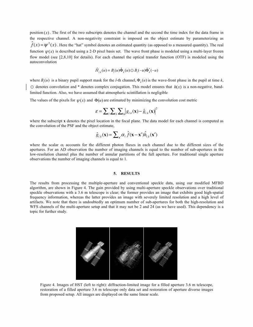
The results from processing the multiple-aperture and conventional speckle data, using our modified MFBD algorithm, are shown in Figure 4. The gain provided by using multi-aperture speckle observations over traditional speckle observations with a 3.6 m telescope is clear; the former provides an image that exhibits good high-spatial frequency information, whereas the latter provides an image with severely limited resolution and a high level of artifacts. We note that there is undoubtedly an optimum number of sub-apertures for both the high-resolution and WFS channels of the multi-aperture setup and that it may not be 2 and 24 (as we have used). This dependency is a topic for further study.

Figure 4. Images of HST (left to right): diffraction-limited image for a filled aperture 3.6 m telescope, restoration of a filled aperture 3.6 m telescope only data set and restoration of aperture diverse images from proposed setup. All images are displayed on the same linear scale.

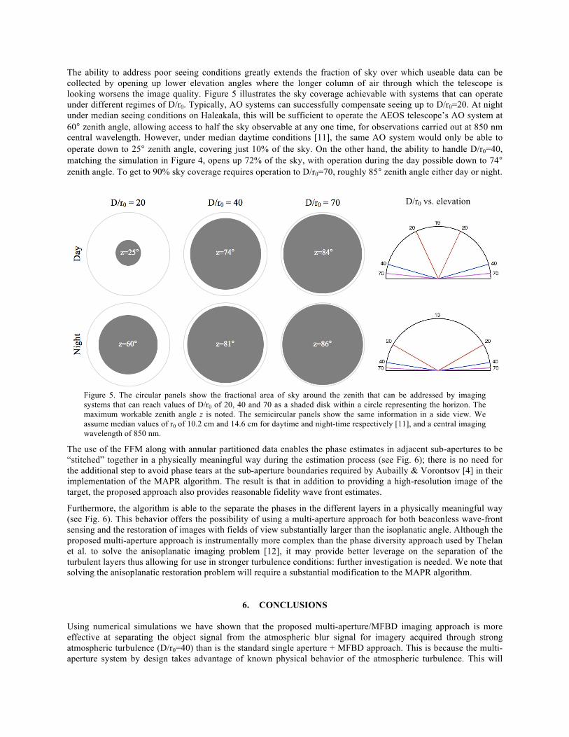
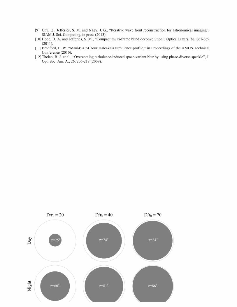
The ability to address poor seeing conditions greatly extends the fraction of sky over which useable data can be collected by opening up lower elevation angles where the longer column of air through which the telescope is looking worsens the image quality. Figure 5 illustrates the sky coverage achievable with systems that can operate under different regimes of D/r0. Typically, AO systems can successfully compensate seeing up to D/r0=20. At night under median seeing conditions on Haleakala, this will be sufficient to operate the AEOS telescope’s AO system at 60° zenith angle, allowing access to half the sky observable at any one time, for observations carried out at 850 nm central wavelength. However, under median daytime conditions [11], the same AO system would only be able to operate down to 25° zenith angle, covering just 10% of the sky. On the other hand, the ability to handle D/r0=40, matching the simulation in Figure 4, opens up 72% of the sky, with operation during the day possible down to 74° zenith angle. To get to 90% sky coverage requires operation to D/r0=70, roughly 85° zenith angle either day or night.

Figure 5. The circular panels show the fractional area of sky around the zenith that can be addressed by imaging systems that can reach values of D/r0 of 20, 40 and 70 as a shaded disk within a circle representing the horizon. The maximum workable zenith angle z is noted. The semicircular panels show the same information in a side view. We assume median values of r0 of 10.2 cm and 14.6 cm for daytime and night-time respectively [11], and a central imaging wavelength of 850 nm.

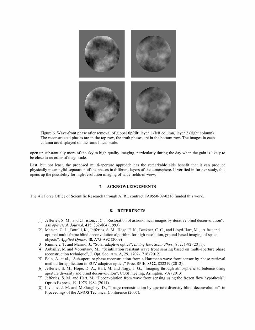
The use of the FFM along with annular partitioned data enables the phase estimates in adjacent sub-apertures to be “stitched” together in a physically meaningful way during the estimation process (see Fig. 6); there is no need for the additional step to avoid phase tears at the sub-aperture boundaries required by Aubailly & Vorontsov [4] in their implementation of the MAPR algorithm. The result is that in addition to providing a high-resolution image of the target, the proposed approach also provides reasonable fidelity wave front estimates.

Furthermore, the algorithm is able to the separate the phases in the different layers in a physically meaningful way (see Fig. 6). This behavior offers the possibility of using a multi-aperture approach for both beaconless wave-front sensing and the restoration of images with fields of view substantially larger than the isoplanatic angle. Although the proposed multi-aperture approach is instrumentally more complex than the phase diversity approach used by Thelan et al. to solve the anisoplanatic imaging problem [12], it may provide better leverage on the separation of the turbulent layers thus allowing for use in stronger turbulence conditions: further investigation is needed. We note that solving the anisoplanatic restoration problem will require a substantial modification to the MAPR algorithm.

6. CONCLUSIONS Using numerical simulations we have shown that the proposed multi-aperture/MFBD imaging approach is more effective at separating the object signal from the atmospheric blur signal for imagery acquired through strong atmospheric turbulence (D/r0=40) than is the standard single aperture + MFBD approach. This is because the multi-aperture system by design takes advantage of known physical behavior of the atmospheric turbulence. This will

D/r0 vs. elevation angle

open up substantially more of the sky to high quality imaging, particularly during the day when the gain is likely to be close to an order of magnitude.

Last, but not least, the proposed multi-aperture approach has the remarkable side benefit that it can produce physically meaningful separation of the phases in different layers of the atmosphere. If verified in further study, this opens up the possibility for high-resolution imaging of wide fields-of-view.

7. ACKNOWLEDGEMENTS

The Air Force Office of Scientific Research through AFRL contract FA9550-09-0216 funded this work.

8. REFERENCES

[1] Jefferies, S. M., and Christou, J. C., "Restoration of astronomical images by iterative blind deconvolution", Astrophysical. Journal, 415, 862-864 (1993)

[2] Matson, C. L., Borelli, K., Jefferies, S. M., Hege, E. K., Beckner, C. C., and Lloyd-Hart, M., “A fast and optimal multi-frame blind deconvolution algorithm for high-resolution, ground-based imaging of space objects”, Applied Optics, 48, A75-A92 (2009)

[3] Rimmele, T. and Marino, J., “Solar adaptive optics”, Living Rev. Solar Phys., 8, 2, 1-92 (2011). [4] Aubailly, M and Vorontsov, M., “Scintillation resistant wave front sensing based on multi-aperture phase

reconstruction technique”, J. Opt. Soc. Am. A, 29, 1707-1716 (2012). [5] Polo, A. et al., “Sub-aperture phase reconstruction from a Hartmann wave front sensor by phase retrieval

method for application in EUV adaptive optics,” Proc. SPIE, 8322, 832219 (2012). [6] Jefferies, S. M., Hope, D. A., Hart, M. and Nagy, J. G., “Imaging through atmospheric turbulence using

aperture diversity and blind deconvolution”, COSI meeting, Arlington, VA (2013) [7] Jefferies, S. M. and Hart, M, “Deconvolution from wave front sensing using the frozen flow hypothesis”,

Optics Express, 19, 1975-1984 (2011). [8] Invanov, J. M. and McGaughey, D., “Image reconstruction by aperture diversity blind deconvolution”, in

Proceedings of the AMOS Technical Conference (2007).

Figure 6. Wave-front phase after removal of global tip/tilt: layer 1 (left column) layer 2 (right column). The reconstructed phases are in the top row, the truth phases are in the bottom row. The images in each column are displayed on the same linear scale.

[9] Chu, Q., Jefferies, S. M. and Nagy, J. G., “Iterative wave front reconstruction for astronomical imaging”, SIAM J. Sci. Computing, in press (2013).

[10] Hope, D. A. and Jefferies, S. M., “Compact multi-frame blind deconvolution”, Optics Letters, 36, 867-869 (2011).

[11] Bradford, L. W. “Maui4: a 24 hour Haleakala turbulence profile,” in Proceedings of the AMOS Technical Conference (2010).

[12] Thelan, B. J. et al., “Overcoming turbulence-induced space-variant blur by using phase-diverse speckle”, J. Opt. Soc. Am. A., 26, 206-218 (2009).

Nig

ht

Day

z=25° z=74° z=84°

z=60° z=81° z=86°

D/r0 = 20 D/r0 = 40 D/r0 = 70