High-resolution global gravity field modelling by the ... · High-resolution global gravity field modelling ... Faculty of Civil Engineering, Slovak University of Technology,

Stud. Geophys. Geod., 59 (2015), 120, DOI: 10.1007/s11200-013-0634-z 1 © 2014 Inst. Geophys. AS CR, Prague

High-resolution global gravity field modelling by the finite volume method

ZUZANA MINARECHOVÁ, MAREK MACÁK, ROBERT ČUNDERLÍK AND KAROL MIKULA

Department of Mathematics and Descriptive Geometry, Faculty of Civil Engineering, Slovak University of Technology, Radlinského 11, 813 68 Bratislava, Slovakia ([email protected], [email protected], [email protected], [email protected])

Received: June 5, 2013; Revised: December 20, 2013; Accepted: June 25, 2014

ABSTRACT

We discuss the parallel computational solution to the modified fixed gravimetric boundary-value problem (MFGBVP). In our approach, the computational domain is a finite space bounded by two spatial boundaries. The boundaries represent an approximation of the Earth’s surface and an approximation of the chosen satellite orbit. Then the MFGBVP consists of the Laplace equation for unknown disturbing potential with the Neumann and Dirichlet boundary conditions. Solution of such elliptic boundary-value problem is understood in a weak sense, so it always exists and is unique. As a numerical method for our parallel approach, the finite volume method (FVM) has been designed and implemented. The FVM is a method for solving elliptic equations and it leads to a solution of the sparse linear system of equations with an appropriate structure for parallel implementation concerning memory costs. The parallel implementation of FVM algorithms using MPI and NUMA procedures is also described. Several numerical experiments are discussed. In the first testing experiment, we show that the proposed approach is second-order accurate. Then we test a convergence of the FVM solution to the EGM2008 Earth gravitational model when refining the grid. In this case all boundary conditions (BCs) are generated from this model. Finally we present high-resolution global gravity field modelling using input data generated from the DTU10 gravity field model and the GOCO03S satellite-only geopotential model. It combines information from the GRACE and GOCE satellite misions prescribed on the upper boundary with the altimetry-derived and terrestrial gravity data available on the Earth’s surface. The obtained global gravity field model is compared with the EGM2008. K e y w o r d s : modified fixed gravimetric boundary-value problem, finite volume

method, parallel computational solution, high-resolution global gravity field modelling

1. INTRODUCTION

A determination of the Earth’s gravity field is one of three fundamental pillars of modern geodesy. It is usually formulated in terms of the geodetic boundary-value problems (BVPs). There exist various numerical approaches to solve such potential problems. For global gravity field modelling, the spherical harmonics based methods are

Z. Minarechová et al.

2 Stud. Geophys. Geod., 59 (2015)

usually used, cf. Pavlis et al. (2012); Bruinsma et al. (2010, unpublished results). This approach, which solves the problem in a frequency domain, has become very efficient and sophisticated tool. However, a recent development of computing facilities has brought new opportunities in numerical solutions to BVPs in physical geodesy. Numerical methods like boundary element method (BEM), finite element method (FEM), finite difference method (FDM) and others allow global modelling in a space domain. Their parallel implementations provide opportunity for high-resolution gravity field modelling. The aforementioned methods have been recently applied for gravity field modelling.

The BEM was innovatively applied in Klees (1992). This approach based on the Galerkin BEM and the indirect BEM formulation was extended by parallel computing (Lehmann and Klees, 1996; Lehmann, 1997) and fast multipole method (Klees et al., 2001). Then Čunderlík et al. (2000), Čunderlík et al. (2008), Čunderlík and Mikula (2010) presented the direct BEM formulation based on the collocation method for solving the linearized fixed gravimetric BVP. In case of the FEM, the pioneering work has been done by Meissl (1981) and Shaofeng and Dingbo (1991). Later, the finite element technique for the solution of gravimetric BVPs with mixed boundary conditions (BCs) in 3D domains above the Earth’s surface was studied in Fašková (2008) and Fašková et al. (2010). The FDM was applied by Keller (1995). Other numerical approaches based on a weak formulation of the BVP and minimization of a quadratic functional were developed in Holota (2005), Nesvadba et al. (2007) and Holota and Nesvadba (2008). In this paper we present a novel computational approach to the global gravity field

modelling based on the finite volume method (FVM). Although the FVM was initially introduced for conservation laws and other uid dynamics problems, nowadays it is used in a broad range of applications. In this study, we use FVM to solve the modified fixed gravimetric BVP (MFGBVP) introduced in Fašková et al. (2010), and we build its new parallel computational solution. For the discretization of MFGBVP we use hexahedraltype grids above the ellipsoid. On contrary to FEM, which gives the numerical scheme with 27-point stencil for this type of grids, the FVM gives 7-point stencil (cf. Eymard et al., 2000) leading to much sparser structure of matrix coefficients and thus yielding 34 times lower memory costs for large-scale computational approaches developed in this paper. Consequently, it allows to perform more detailed computations using FVM grid in comparison to FEM grid with the same memory costs. Since both FEM and FVM are second order accurate methods, the lower memory requirements represent a strong advantage of FVM in our application. Parallel implementation using the MPI (Message Passing Interface) procedures and an

optimization of communications on parallel computers with the NUMA (Non-Uniform Memory Access) architecture has been performed and its description is presented. The implementation includes splitting of all arrays in the meridional direction as well as usage of the parallel Bi-CGSTAB non-stationary iterative solver. Together they provide an efficient tool for the high-resolution modelling in a space domain, where a level of the discretization practically depends on a capacity of available high performance computing (HPC) facilities. Our motivation is to develop an efficient approach to detailed global gravity field

modelling in the space domain that would be able to achieve the same high level of resolution as input data are provided in. At present, the available datasets of altimetry-

High-resolution global gravity field modelling …

Stud. Geophys. Geod., 59 (2015) 3

derived gravity data are provided in 1 1 grids and they are repeatedly updated using new information from satellite altimeters, e.g. the DNSC08-GRA (Andersen et al., 2010), DTU10-GRA (Andersen, 2010) and recently DTU13-GRA (Andersen et al., 2013, unpublished results), or the datasets provided by Sandwell and Smith, versions 18.1-21.1, see Sandwell and Smith (2009), or Sandwell et al. (2013, unpublished results). At oceans, which represent almost 70% of the Earth’s surface, these datasets provide altimetry-derived gravity data in the high-resolution based on the precise satellite altimetry. To capture such detailed information it is very natural to solve the problem in the space domain. A main advantage of the presented approach is that it can be applied very straightforwardly for such high-resolution input data leading to large-scale parallel computations. To utilise information from the satellite missions like GRACE or GOCE, the FVM solutions to the proposed MFGBVP are fixed on the upper boundary, which is considered at average altitude of the GOCE orbits. Here the Dirichlet BC is prescribed and it can be generated from any GRACE/GOCE based satellite-only geopotential model. To demonstrate behaviour and properties of the proposed FVM approach we present

several numerical experiments. In Subsection 4.1 we test properties of the FVM scheme in numerical experiments representing potential generated by a homogeneous sphere. The obtained FVM solutions are compared with the exact solution testing the order of convergence. In Subsection 4.2 we solve the MFGBVP where all BCs as input data are generated from EGM2008 geopotential model up to degree 2160 (Pavlis et al., 2012). Our aim is to show that the obtained FVM solutions converge to EGM2008 when refining the FVM grid. In Subsection 4.3 we deal with the high-resolution global gravity field modelling using input data generated from available altimetry-derived gravity datasets. The FVM solution is fixed on the upper boundary at altitude of 240 km above the reference ellipsoid by the Dirichlet BC generated from the GOCO03S satellite-only geopotential model (Mayer-Gürr et al., 2012). The input gravity disturbances on the Earth’s surface as the Neumann BC are interpolated from the DTU10 gravity field model. The obtained FVM solutions represent high-resolution gravity field models that are compared with EGM2008.

2. FORMULATION OF THE MODIFIED FIXED GRAVIMETRIC BOUNDARY-VALUE PROBLEM

Let us consider the fixed gravimetric boundary-value problem (FGBVP), cf. Koch and Pope (1972), Holota (1997), Čunderlík et al. (2008):

0T x , 3R S x , (1)

,T g x sx x, x S , (2)

0T x as x , (3)

where S is the Earth’s body, T x is the disturbing potential defined as the difference

between the real W x and the normal U x gravity potential at any point x, g x is



the so-called gravity disturbance and U U sx x x is the unit vector

normal to the equipotential surface of the normal potential U at point x. Although the previously described FGBVP (Eqs (1)(3)) deals with the infinite

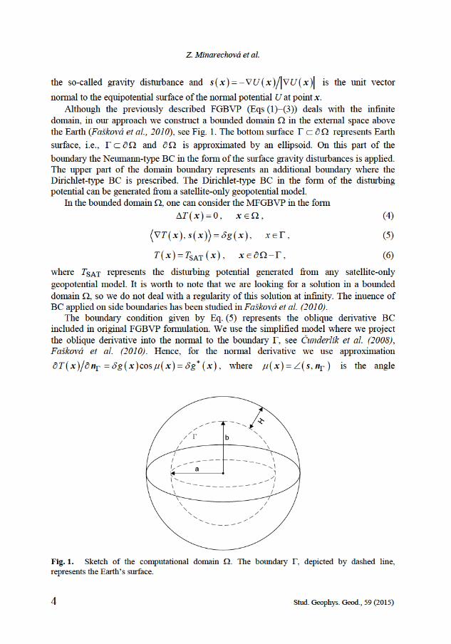
domain, in our approach we construct a bounded domain in the external space above the Earth (Fašková et al., 2010), see Fig. 1. The bottom surface represents Earth

surface, i.e., and is approximated by an ellipsoid. On this part of the

boundary the Neumann-type BC in the form of the surface gravity disturbances is applied. The upper part of the domain boundary represents an additional boundary where the Dirichlet-type BC is prescribed. The Dirichlet-type BC in the form of the disturbing potential can be generated from a satellite-only geopotential model. In the bounded domain , one can consider the MFGBVP in the form

0T x , x , (4)

,T g x sx x, x, (5)

SATT Tx x, x , (6)

where TSAT represents the disturbing potential generated from any satellite-only

geopotential model. It is worth to note that we are looking for a solution in a bounded domain , so we do not deal with a regularity of this solution at infinity. The inuence of BC applied on side boundaries has been studied in Fašková et al. (2010). The boundary condition given by Eq. (5) represents the oblique derivative BC

included in original FGBVP formulation. We use the simplified model where we project the oblique derivative into the normal to the boundary , see Čunderlík et al. (2008), Fašková et al. (2010). Hence, for the normal derivative we use approximation

cosT g g x n x x x, where , x sn is the angle

Fig. 1. Sketch of the computational domain . The boundary , depicted by dashed line, represents the Earth’s surface.



between s and n. It is worth to note that a new quantity g x represents the

projection of the vector g xsx to the normal n and not a projection of the gradient

T x onto this normal.

Consequently, in our approach presented in this paper we solve the following form of MFGBVP:

0T x , x , (7)

T

g

xx

n, x, (8)

SATT Tx x, x . (9)

It is important to note that the solution of Eqs (7)(9) is understood in a weak sense. Such a solution is a generalization of classical solutions, coincides with them in a smooth case, and nowadays it is used in study of BVP for partial differential equations, see e.g. Brenner and Scott (2002), Eymard et al. (2000). To derive the weak formulation of Eqs (7)(9), we define the Sobolev space of test

functions V that is the space of functions from 12W which are equal to 0 on ,

in the sense of traces, cf. Brenner and Scott (2002). We multiply the differential equation

(7) by Vv and integrate in . By Green’s theorem we get

, , 0T dx T dx

nv v , V v , (10)

where n is a unit outer normal to .

Let the extension of Dirichlet BC given by TSAT into the domain be in 12W

and let 2g L . Then we define a weak solution of our MFGBVP (Eqs (7)(9)) as

a function T, such that SATT T V and following identity holds

, 0T dx g dx

v v , V v . (11)

According to Brenner and Scott (2002) or Rektorys (1980), the solution of this problem always exists and is unique.

3. SOLUTION OF THE MODIFIED FIXED GRAVIMETRIC BOUNDARY-VALUE PROBLEM BY THE FINITE VOLUME METHOD

In FVM we divide the computational domain into a number of finite volumes p. We multiply the Laplace equation by minus one and then by integrating Eq. (7) over a finite volume and using the divergence theorem



,p p

Tdx T dx

n , (12)

we obtain for every finite volume p

0

p

Tdxn

. (13)

Let pq N be a neighbor of the finite volume p, where we have denoted by Np all

neighbors which have common side with p. Then let Tp and Tq be the approximate values

of T in p and q, epq is a boundary of the finite volume p common with q, pqn is its unit

normal vector oriented from p to q, and pqme is the area of epq. Let xp and xq be

representative points of p and q (e.g. centers of gravity) and dpq their mutual distance. If

we approximate the normal derivative along the boundary of volume p by

q p

pq pq

T TT

n d

, (14)

from Eqs (13) and (14) for every finite volume p we obtain

0p

q ppq

q N pq

T Tme

d

. (15)

Finally, after rearrangement we have

0p

pqp q

q N pq

meT T

d

, (16)

which represents the linear system of algebraic equations for FVM. The term

pq pqme d defined for the finite volume p and its neighbor q is referred to as the

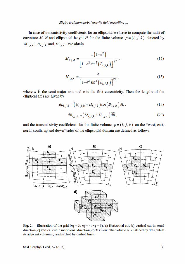
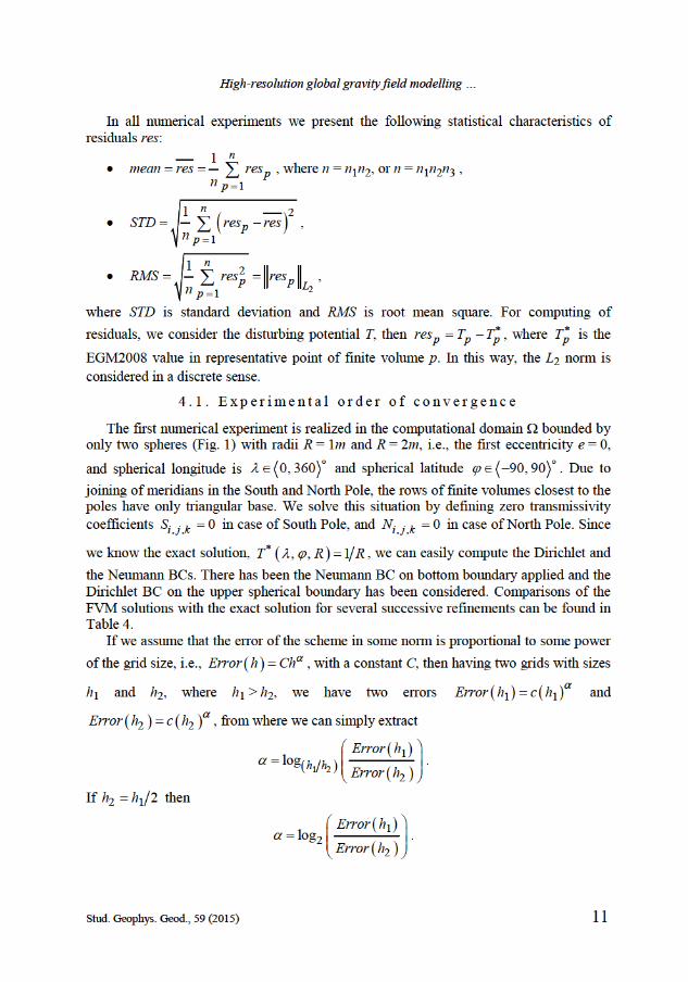
transmissivity coefficient, see e.g. Eymard et al. (2000). The system given by Eq. (16) must be accompanied by boundary conditions. To do that we consider an extension of our finite volume grid by one row of finite volumes which will be used for application of BCs. More details about this treatment will be discussed later. Now we restrict to the specific situation depicted in Fig. 2. We define indices

i = 1, …, n1, j = 1, …, n2 and k = 1, …, n3 in the direction of the geodetic longitude L,

geodetic latitude B and height H. Then the lengths of the segments in geodetic coordinates

are 1u ddL L L n , 2u ddB B B n and 3udH H n (Hd = 0), where Lu, Bu

and Hu denote the upper boundary of the range of longitude, latitude and radius, Ld, Bd

and Hd their lower boundaries, respectively.



In case of transmissivity coefficients for an ellipsoid, we have to compute the radii of

curvature M, N and ellipsoidal height H for the finite volume ,,p ijk denoted by

,,ijkM , ,,ijkN and ,,ijkH . We obtain

2

,, 322 2,,

1

1 sinijk

ijk

a eM

e B

, (17)

,, 122 2

,,1 sinijk

ijk

aN

e B

, (18)

where a is the semi-major axis and e is the first eccentricity. Then the lengths of the elliptical arcs are given by

,, ,, ,, ,,cosijk ijk ijk ijkdL N H B dL , (19)

,, ,, ,,ijk ijk ijkdB M H dB , (20)

and the transmissivity coefficients for the finite volume ,,p ijk on the “west, east,

north, south, up and down” sides of the ellipsoidal domain are defined as follows

Fig. 2. Illustration of the grid (n1 = 3; n2 = 4; n3 = 5). a) Horizontal cut, b) vertical cut in zonal

direction, c) vertical cut in meridional direction, d) 3D view. The volume p is hatched by dots, while its adjacent volumes q are hatched by dashed lines.



12 , , 12 , ,,, ,,

,, ,,

, 12, , 12,,, ,,

,, ,,

, , 12 , , 12 , , 12 , , 12,, ,,

,, ,, ,, ,, ,

, ,

, ,

, ,

i jk i jkijk ijk

ijk ijk

ij k ij kijk ijk

ijk ijk

ijk ijk ijk ijkijk ijk

ijk ijk ijk ijk ij

dB dH dB dHW E

dL dL

dL dH dL dHS N

dB dB

dB dL dB dLD U

dH dH

P W E N S

, ,, ,,.k ijk ijkU D

(21)

Finally, with these definitions of coefficients we have to solve the linear system given by Eq. (16) in the form

,, ,, ,, 1,, ,, 1,, ,, , 1,

,, , 1, ,, ,, 1 ,, ,, 1 0.

ijk ijk ijk i jk ijk i jk ijk ij k

ijk ij k ijk ijk ijk ijk

P T W T E T N T

S T U T D T

(22)

The system of coefficients and the right-hand side vector is modified for finite volumes along boundary of the computational domain. It is done in the following way. For volumes along side and upper boundaries, case of the Dirichlet BCs, we prescribe the

disturbing potential TSAT for Tq in Eq. (16), and move the term pq pq qme d T to

the right-hand side. For the Neumann-type BCs applied on the bottom boundary, we

prescribe g for the value q p pqT T d in Eq. (16), see also Eq. (14), and move

pqme g to the right-hand side and update the diagonal coefficient to

,, ,, ,, ,, ,, ,,ijk ijk ijk ijk ijk ijkP W E N S U . Using these approaches, we get the

right-hand side vector with nonzero entries and modified diagonal coefficients for finite volumes along the boundary. Then the system matrix is nonsymmetric and diagonal dominant.

3.1. Iterative solvers

The linear system of algebraic equations (22) is written in the form

x bA , (23)

where A is a matrix with given coefficients (Eq. (21)), b is a right-hand side vector and x is an unknown vector. Stationary iterative methods like the Gauss-Seidel or SOR (Successive-Over Relaxation) are easy to implement, but usually not so efficient for solving elliptic problems, cf. Fašková (2008), Table 1. We use nonstationary methods that are based on the idea of sequences of orthogonal vectors. The nonstationary methods like Bi-CGSTAB (BiConjugate Gradient Stabilized) differ

from stationary ones by the fact that the computations involve information that changes in each iteration, see Sleijpen and Fokkema (1993). Typically, new updates are computed by

taking inner products of residuals kx bA , where kx is a current iteration, or other



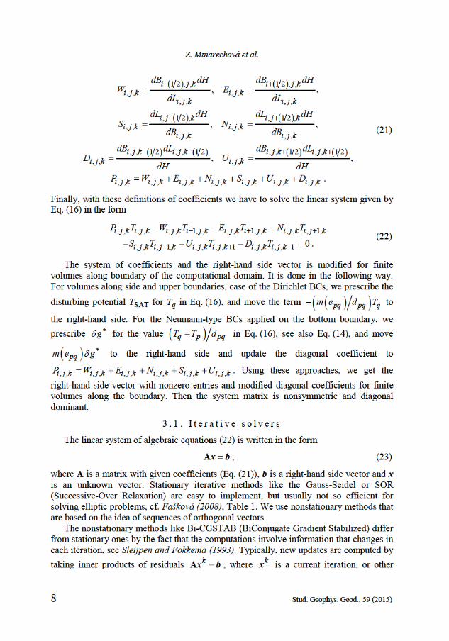
vectors arising in the iterative procedure. In our approach, we have chosen the Bi-CGSTAB method, cf. Sleijpen and Fokkema (1993), which is robust and stable method developed for solving nonsymmetric linear systems of equations and we have implemented and optimized it for our sparse matrix. In comparison with all methods tested in this study, Bi-CGSTAB has the lowest memory requirements as well as the overall CPU time due to lowest number of iterations (Table 2).

3.2. Parallelization of the method

Nowadays, the speed up of numerical algorithms can be performed by distributing of computations into several processes using the so-called Massively Parallel Processors (MPP) architecture together with the Message Passing Interface (MPI) programming framework. In our applications we use Single Program Multiple Data model, where only one

program is built to run on each process and working with different part of data sets. Each process has its own unique integer identifier assigned by the system when the process initializes. The communication between processors is managed by the MPI functions. When performing large-scale computations on clusters with the NUMA architecture,

the computational time can be significantly reduced using the NUMA optimizations allocating memory with the fastest access to each processor. An optimal utilization of the NUMA functions in our applications using Bi-CGSTAB (see Section 3.1) can reduce computational time by 50% in comparison to the same computation without the NUMA functions, cf. Špir (2012).

Table 1. Efficiency comparison of the stationary and nonstationary methods in the experiment with size n1 n2 n3 = 500 300 100, tested on one processor.

Solver CPU Time [s] Number of Iterations

SOR 1.10724e+05 70000 Bi-CGSTAB 4.65251e+03 1100

Table 2. The average memory and time costs for various BiCG linear solvers, where APXY is the number of vector scalar products, DOT is a number of scalar-vector multiplications, MEM represents a number of additional vectors needed in iterative procedure, ITER gives a number of iterations to reach the prescribed residual and TIME presents the overall CPU time in seconds. The table is constructed for a particular nonsymmetric matrix from our finite volume method, and from MEM and TIME columns one can see optimality of Bi-CGSTAB. BiCGstab(l) denotes Bi-CGSTAB restarted at each l-th step.

APXY DOT MEM ITER TIME

Bi-CG 6.50 2.00 7 1123 1203 Bi-CGASTAB 3.00 2.00 7 567 691 BiCGASTAB(2) 5.50 2.27 9 648 833 Bi-CGASTAB(4) 5.25 5.75 13 446 902



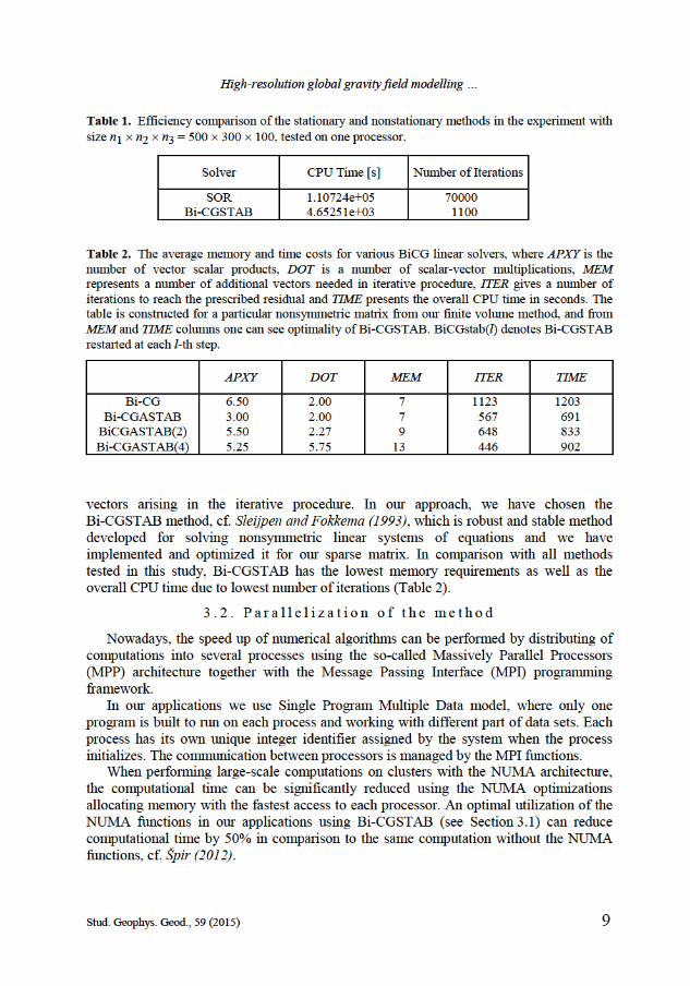
There exist several possibilities of data management in parallel implementations, see Aoyama and Nakano (1999). In our parallel algorithms we split all the multidimensional arrays (e.g. matrix coefficients, right-hand side vector, solution vector) into sections which can be allocated in the memory of single processor. In order to solve the linear system iteratively, we have created overlapping 2D slices which are used to exchange solution after each iteration for splitting in radial (Case a) and in meridional (Case b) directions, see Fig. 3. Splitting given by case a was used in Fašková (2008). However, in numerical experiments presented in this work, where the number of divisions in radial direction is significantly lower than in other two directions, it is more appropriate to use Case b, because 2D slices which must be communicated have smaller dimensions in this case. To illustrate this fact we present Table 3. It reports large differences in communicated memory in case of using different splitting. This difference in data communications between processors (cores) brings the triple overall speed up for our large-scale experiments.

4. NUMERICAL EXPERIMENTS

In this section we present numerical experiments where we solve the BVP given by Eqs (7)(9) by the FVM discussed above. First we study the experimental order of convergence of our approach. Afterwards, we present the global gravity field modeling where all input BCs are generated from EGM2008 and a convergence of our results to EGM2008 is studied. Then we apply the proposed approach using data generated from DTU10-GRAV and GOCO03S.

Fig. 3. Different types for data splitting and overlapping over parallel processes: a) radial split of the domain, b) meridional split of the domain.

Table 3. Comparison of the communication memory cost (in MB) for different data splitting in two numerical experiments.

Size of Experiment Radial Split Meridional Split

4200 2400 120 576.78 16.47

790 300 100 13.56 1.71



In all numerical experiments we present the following statistical characteristics of residuals res:

1

1 n

pp

mean res resn

, where n = n1n2, or n = n1n2n3 ,

2

1

1 n

pp

STD res resn

,

2

2

1

1 n

p pLp

RMS res resn

,

where STD is standard deviation and RMS is root mean square. For computing of

residuals, we consider the disturbing potential T, then p p pres T T , where pT is the

EGM2008 value in representative point of finite volume p. In this way, the L2 norm is

considered in a discrete sense.

4.1. Experimental order of convergence

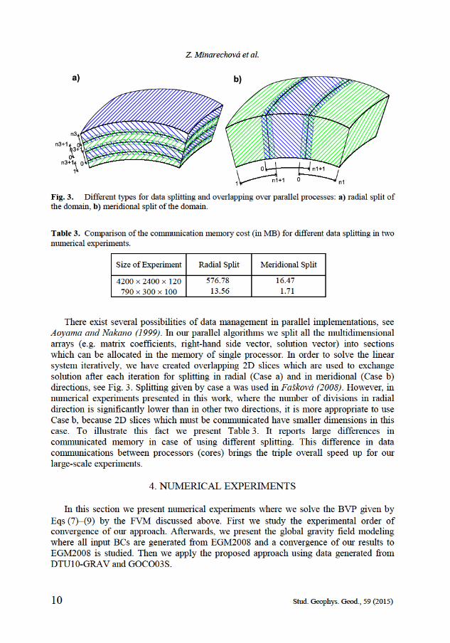
The first numerical experiment is realized in the computational domain bounded by only two spheres (Fig. 1) with radii R = 1m and R = 2m, i.e., the first eccentricity e = 0,

and spherical longitude is 0, 360 and spherical latitude 90, 90

. Due to

joining of meridians in the South and North Pole, the rows of finite volumes closest to the poles have only triangular base. We solve this situation by defining zero transmissivity coefficients ,, 0ijkS in case of South Pole, and ,, 0ijkN in case of North Pole. Since

we know the exact solution, ,, 1T R R , we can easily compute the Dirichlet and

the Neumann BCs. There has been the Neumann BC on bottom boundary applied and the Dirichlet BC on the upper spherical boundary has been considered. Comparisons of the FVM solutions with the exact solution for several successive refinements can be found in Table 4. If we assume that the error of the scheme in some norm is proportional to some power

of the grid size, i.e., Error h Ch , with a constant C, then having two grids with sizes

h1 and h2, where h1 > h2, we have two errors 1 1Error h c h

and

2 2Error h c h

, from where we can simply extract

1 2

1

2

loghhError h

Error h

.

If 2 12h h then

1

22

logError h

Error h

.



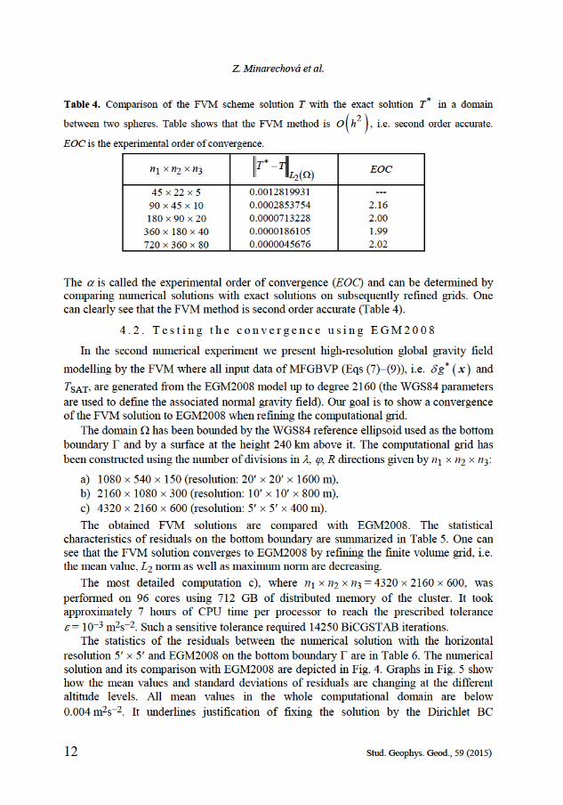
The is called the experimental order of convergence (EOC) and can be determined by comparing numerical solutions with exact solutions on subsequently refined grids. One can clearly see that the FVM method is second order accurate (Table 4).

4.2. Testing the convergence using EGM2008

In the second numerical experiment we present high-resolution global gravity field

modelling by the FVM where all input data of MFGBVP (Eqs (7)(9)), i.e. g x and

TSAT, are generated from the EGM2008 model up to degree 2160 (the WGS84 parameters

are used to define the associated normal gravity field). Our goal is to show a convergence of the FVM solution to EGM2008 when refining the computational grid. The domain has been bounded by the WGS84 reference ellipsoid used as the bottom

boundary and by a surface at the height 240 km above it. The computational grid has been constructed using the number of divisions in , , R directions given by n1 n2 n3:

a) 1080 540 150 (resolution: 20 20 1600 m), b) 2160 1080 300 (resolution: 10 10 800 m), c) 4320 2160 600 (resolution: 5 5 400 m).

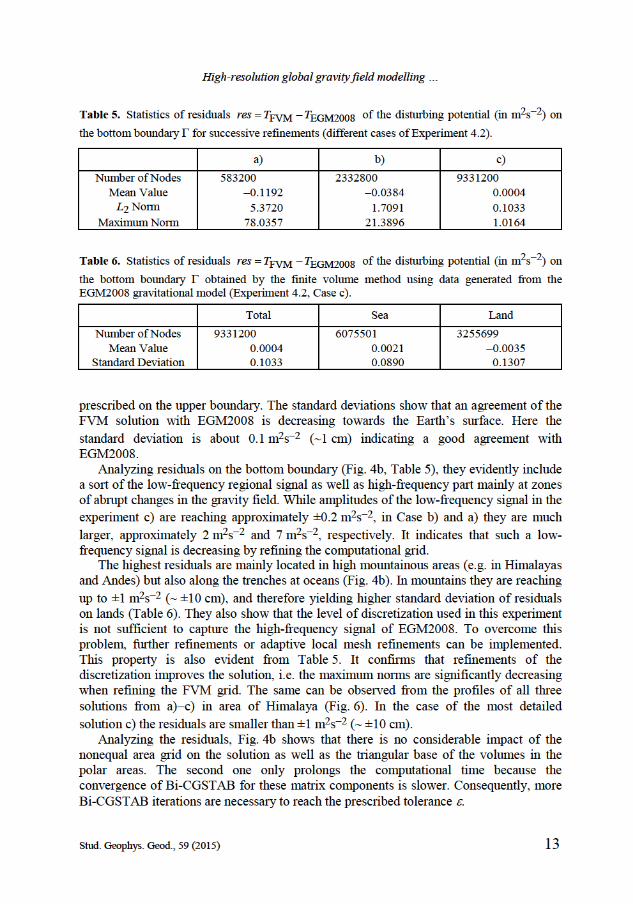
The obtained FVM solutions are compared with EGM2008. The statistical characteristics of residuals on the bottom boundary are summarized in Table 5. One can see that the FVM solution converges to EGM2008 by refining the finite volume grid, i.e. the mean value, L2 norm as well as maximum norm are decreasing.

The most detailed computation c), where n1 n2 n3 = 4320 2160 600, was

performed on 96 cores using 712 GB of distributed memory of the cluster. It took approximately 7 hours of CPU time per processor to reach the prescribed tolerance

= 103 m2s2. Such a sensitive tolerance required 14250 BiCGSTAB iterations. The statistics of the residuals between the numerical solution with the horizontal

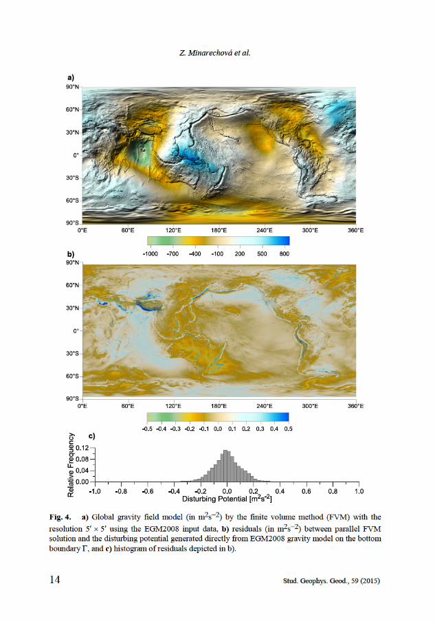
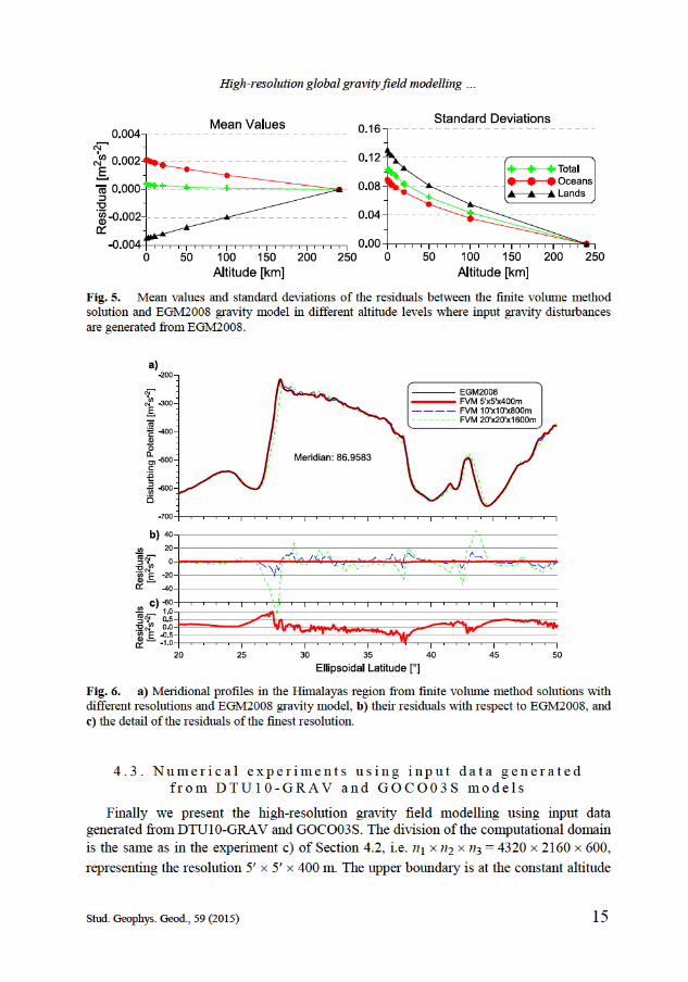
resolution 5 5 and EGM2008 on the bottom boundary are in Table 6. The numerical solution and its comparison with EGM2008 are depicted in Fig. 4. Graphs in Fig. 5 show how the mean values and standard deviations of residuals are changing at the different altitude levels. All mean values in the whole computational domain are below

0.004 m2s2. It underlines justification of fixing the solution by the Dirichlet BC

Table 4. Comparison of the FVM scheme solution T with the exact solution T in a domain

between two spheres. Table shows that the FVM method is 2Oh , i.e. second order accurate.

EOC is the experimental order of convergence.

n1 n2 n3 2LTT

EOC

45 22 5 0.0012819931 ---

90 45 10 0.0002853754 2.16

180 90 20 0.0000713228 2.00

360 180 40 0.0000186105 1.99

720 360 80 0.0000045676 2.02



prescribed on the upper boundary. The standard deviations show that an agreement of the FVM solution with EGM2008 is decreasing towards the Earth’s surface. Here the

standard deviation is about 0.1 m2s2 (1 cm) indicating a good agreement with EGM2008. Analyzing residuals on the bottom boundary (Fig. 4b, Table 5), they evidently include

a sort of the low-frequency regional signal as well as high-frequency part mainly at zones of abrupt changes in the gravity field. While amplitudes of the low-frequency signal in the

experiment c) are reaching approximately ±0.2 m2s2, in Case b) and a) they are much

larger, approximately 2 m2s2 and 7 m2s2, respectively. It indicates that such a low-frequency signal is decreasing by refining the computational grid. The highest residuals are mainly located in high mountainous areas (e.g. in Himalayas

and Andes) but also along the trenches at oceans (Fig. 4b). In mountains they are reaching

up to ±1 m2s2 ( ±10 cm), and therefore yielding higher standard deviation of residuals on lands (Table 6). They also show that the level of discretization used in this experiment is not sufficient to capture the high-frequency signal of EGM2008. To overcome this problem, further refinements or adaptive local mesh refinements can be implemented. This property is also evident from Table 5. It confirms that refinements of the discretization improves the solution, i.e. the maximum norms are significantly decreasing when refining the FVM grid. The same can be observed from the profiles of all three solutions from a)c) in area of Himalaya (Fig. 6). In the case of the most detailed

solution c) the residuals are smaller than ±1 m2s2 ( ±10 cm). Analyzing the residuals, Fig. 4b shows that there is no considerable impact of the

nonequal area grid on the solution as well as the triangular base of the volumes in the polar areas. The second one only prolongs the computational time because the convergence of Bi-CGSTAB for these matrix components is slower. Consequently, more Bi-CGSTAB iterations are necessary to reach the prescribed tolerance .

Table 5. Statistics of residuals FVM EGM2008res T T of the disturbing potential (in m2s2) on

the bottom boundary for successive refinements (different cases of Experiment 4.2).

a) b) c)

Number of Nodes 583200 2332800 9331200 Mean Value 0.1192 0.0384 0.0004 L2 Norm 5.3720 1.7091 0.1033

Maximum Norm 78.0357 21.3896 1.0164


the bottom boundary obtained by the finite volume method using data generated from the EGM2008 gravitational model (Experiment 4.2, Case c).

Total Sea Land

Number of Nodes 9331200 6075501 3255699 Mean Value 0.0004 0.0021 0.0035

Standard Deviation 0.1033 0.0890 0.1307



Fig. 4. a) Global gravity field model (in m2s2) by the finite volume method (FVM) with the

resolution 5 5 using the EGM2008 input data, b) residuals (in m2s2) between parallel FVM solution and the disturbing potential generated directly from EGM2008 gravity model on the bottom boundary , and c) histogram of residuals depicted in b).



4.3. Numerical experiments using input data generated from DTU10-GRAV and GOCO03S models

Finally we present the high-resolution gravity field modelling using input data generated from DTU10-GRAV and GOCO03S. The division of the computational domain is the same as in the experiment c) of Section 4.2, i.e. n1 n2 n3 = 4320 2160 600,

representing the resolution 5 5 400 m. The upper boundary is at the constant altitude

Fig. 5. Mean values and standard deviations of the residuals between the finite volume method solution and EGM2008 gravity model in different altitude levels where input gravity disturbances are generated from EGM2008.

Fig. 6. a) Meridional profiles in the Himalayas region from finite volume method solutions with different resolutions and EGM2008 gravity model, b) their residuals with respect to EGM2008, and c) the detail of the residuals of the finest resolution.



240 km above the reference ellipsoid. Here the Dirichlet BCs in form of the disturbing potential are generated from the GOCO03S satellite-only geopotential model up to degree 250. The bottom boundary is represented by the WGS84 reference ellipsoid. Here the input data are prescribed in the form of the gravity disturbances that are transformed from the free-air gravity anomalies interpolated from the DTU10-GRAV dataset provided in

1 1 grid. To transform the DTU10 gravity anomalies g into the gravity disturbances

g we use the relation

EGM20080.3086 mGalg g , (24)

where EGM2008 is the height anomaly evaluated from EGM2008. Here we would like to

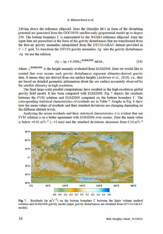
remind that over oceans such gravity disturbances represent altimetry-derived gravity data. It means they are derived from sea surface heights (Andersen et al., 2010), i.e., they are based on detailed geometric information about the sea surface accurately observed by the satellite altimetry in high resolution. The final large-scale parallel computations have resulted in the high-resolution global

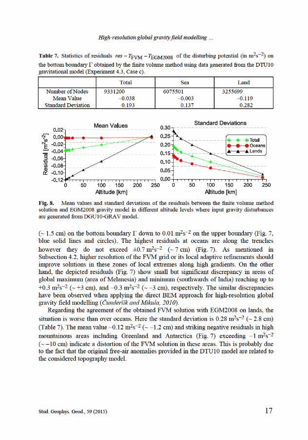
gravity field model. It has been compared with EGM2008. Fig. 7 depicts the residuals between the FVM solution and EGM2008 computed on the bottom boundary . The corresponding statistical characteristics of residuals are in Table 7. Graphs in Fig. 8 show how the mean values of residuals and their standard deviations are changing depending on the different altitude levels. Analyzing the arisen residuals and their statistical characteristics it is evident that our

FVM solution is in a better agreement with EGM2008 over oceans. Here the mean value

is below ±0.01 m2s2 ( ±1 mm) and the standard deviations decreases from 0.14 m2s2

Fig. 7. Residuals (in m2s2) on the bottom boundary between the finite volume method solution and EGM2008 gravity model (input gravity disturbances are obtained from DTU10-GRAV model).



( 1.5 cm) on the bottom boundary down to 0.01 m2s2 on the upper boundary (Fig. 7, blue solid lines and circles). The highest residuals at oceans are along the trenches

however they do not exceed ±0.7 m2s2 ( 7 cm) (Fig. 7). As mentioned in Subsection 4.2, higher resolution of the FVM grid or its local adaptive refinements should improve solutions in these zones of local extremes along high gradients. On the other hand, the depicted residuals (Fig. 7) show small but significant discrepancy in areas of global maximum (area of Melanesia) and minimum (southwards of India) reaching up to

+0.3 m2s2 ( +3 cm), and 0.3 m2s2 ( 3 cm), respectively. The similar discrepancies have been observed when applying the direct BEM approach for high-resolution global gravity field modelling (Čunderlík and Mikula, 2010). Regarding the agreement of the obtained FVM solution with EGM2008 on lands, the

situation is worse than over oceans. Here the standard deviation is 0.28 m2s2 ( 2.8 cm)

(Table 7). The mean value 0.12 m2s2 ( 1.2 cm) and striking negative residuals in high

mountainous areas including Greenland and Antarctica (Fig. 7) exceeding 1 m2s2 ( 10 cm) indicate a distortion of the FVM solution in these areas. This is probably due to the fact that the original free-air anomalies provided in the DTU10 model are related to the considered topography model.


the bottom boundary obtained by the finite volume method using data generated from the DTU10 gravitational model (Experiment 4.3, Case c).

Total Sea Land

Number of Nodes 9331200 6075501 3255699 Mean Value 0.038 0.003 0.119

Standard Deviation 0.193 0.137 0.282

Fig. 8. Mean values and standard deviations of the residuals between the finite volume method solution and EGM2008 gravity model in different altitude levels where input gravity disturbances are generated from DGU10-GRAV model.



5. CONCLUSIONS

In this paper we present new parallel computational method for high-resolution global gravity field modelling. The finite volume method (FVM) has been developed to solve the modified mixed gravimetric bouday-value problem (BVP) in 3D domains above the Earth’s surface approximated by the reference ellipsoid. The FVM solutions are fixed to the low-frequency part precisely obtained from the GRACE/GOCE satellite-only geopotential models. This low-frequency part is prescribed on the upper boundary of the 3D computational domain that is approximately at altitude of the GOCE orbits. Such an approach aims to utilize information from the satellite missions at altitudes of their measurements. The developed approach has been designed to allow processing available datasets of

gravity data provided on the Earth’s surface in high resolution, e.g. altimetry-derived gravity data. To capture such detailed information it is very natural to solve the problem in the space domain. A main advantage of the presented approach is that it can be applied very straightforwardly for such high-resolution input data, although leading to large-scale parallel computations. The parallel implementation of algorithms using the MPI procedures and large-scale

parallel computations on clusters with the distributed memory aims to reach high level of the discretization. An advantage of the FVM is that it gives 7-point stencil leading to much sparser structure of matrix coefficients than the finite element method. This fact yields 34 times lower memory costs for large-scale computational approaches. Consequently, the FVM allows to perform more detailed computations in comparison to the finite element method with the same memory costs. The proposed parallelization includes splitting of all arrays in the meridional direction, a parallel implementation of the Bi-CGSTAB non-stationary iterative solver and an optimization of communications on parallel computers with the NUMA architecture. All these aspects increase efficiency of the proposed approach to high-resolution gravity field modelling where a level of the discretization practically depends on available HPC facilities. The presented numerical experiments show that our FVM method is second order

accurate. In case when all input data are generated from EGM2008, the FVM solution converges to EGM2008 by refining the finite volume grid. The standard deviation of

about 0.1 m2s2 and the mean value 0.0004 m2s2 on the bottom boundary in case of the horizontal resolution 5 5 indicates a good agreement with EGM2008. Moreover, maximum norms are significantly decreasing when refining the grid. Hence, the further refinements should improve the obtained solution. In case of the high-resolution gravity field modelling using input data generated from

the DTU10 dataset, the obtained FVM solutions is also in a good agreement with

EGM2008, especially over oceans (the standard deviation is 0.14 m2s2 and the mean

value is below ±0.01 m2s2). Taking into account that such input data over oceans represent altimetry-derived gravity data that differ from those used for a compilation of EGM2008, such a good agreement confirms efficiency of our proposed approach. This can be promising for detail processing of available altimetry-derived gravity datasets provided in high resolution. An aforementioned advantage of straightforward refinements of the discretization is giving an opportunity to achieve the FVM solutions with the same



high resolution as input data are provided in. In this way very detailed information about the gravity field over oceans observed by satellite altimetry can be captured providing original data useful for other applications like modelling of the mean dynamic topography, deriving velocities of the ocean geostrophic surface currents or determination of the W0 estimates.

Acknowledgments: This work was supported by grant APVV-0072-11 and VEGA 1/1063/11.

Calculations were performed in the Computing Center of the Slovak Academy of Sciences using the supercomputing infrastructure acquired in project ITMS 26240120025 (Slovak infrastructure for high-performance computing) supported by the Research and Development Operational Programme funded by the ERDF.

References

Andersen O.B., Knudsen P. and Berry P., 2010. The DNSC08-GRAV global marine gravity field from double retracked satellite altimetry. J. Geodesy, 84, 191199.

Andersen O.B., 2010. The DTU10 gravity field and mean sea surface - improvements in the Arctic. Second International Symposium of the Gravity Field of the Earth (IGFS2), Fairbanks, Alaska (http://www.space.dtu.dk/english/%7E/media/Institutter/Space/English/scientific_data_and_models/global_marine_gravity_field/dtu10.ashx).

Aoyama Y. and Nakano J., 1999. RS/6000 SP: Practical MPI Programming. IBM, www.redbooks.ibm.com.

Brenner S.C. and Scott L.R., 2002. The Mathematical Theory of Finite Element Methods. 2nd Edition. Springer-Verlag, New York.

Čunderlík R., Mikula K. and Mojzeš M., 2002. The boundary element method applied to the determination of the global quasigeoid. In: Handlovičová A., Krivá Z., Mikula K. and Ševčovič D. (Eds.), Proceedings of ALGORITMY 2002, Conference on Scientific Computing. Faculty of Civil Engineering, Slovak University of Technology, Bratislava, Slovakia, 301308, ISBN: 80-227-1750-9.

Čunderlík R., Mikula K. and Mojzeš M., 2008. Numerical solution of the linearized fixed gravimetric boundary-value problem. J. Geodesy, 82, 1529.

Čunderlík R. and Mikula K., 2010. Direct BEM for high-resolution global gravity field modelling. Stud. Geophys. Geod., 54, 219238.

Eymard R., Gallouët T. and Herbin R., 2000. Finite volume methods. In: Ciarlet P.G. and Lions J.L. (Eds), Handbook for Numerical Analysis, Vol. 7. Elsevier, Amsterdam, The Netherlands.

Fašková Z., 2008. Numerical Methods for Solving Geodetic Boundary Value Problems. Ph.D. Thesis, Faculty of Civil Engineering, Slovak University of Technology, Bratislava, Slovakia.

Fašková Z., Čunderlík R. and Mikula K., 2010. Finite element method for solving geodetic boundary value problems. J. Geodesy, 84, 135144.

Holota P., 1997. Coerciveness of the linear gravimetric boundary-value problem and a geometrical interpretation. J. Geodesy, 71, 640651.

Holota P., 2005. Neumann’s boundary-value problem in studies on Earth gravity field: weak solution. In: Holota P. and Slaboch V. (Eds), 50 years of Research Institute of Geodesy, Topography and Cartography, Prague. Research Institute of Geodesy, Topography and Cartography, Vol. 50, No. 36, 4969.



Holota P. and Nesvadba O., 2008. Model refinements and numerical solution of weakly formulated boundary-value problems in physical geodesy. In: Xu P., Liu J. and Dermanis A. (Eds), VI Hotine-Marussi Symposium on Theoretical and Computational Geodesy. International Association of Geodesy Symposia 132. Springer-Verlag, Berlin, Germany, 320326.

Keller W., 1995. Finite differences schemes for elliptic boundary value problems. Section IV Bulletin IAG, No. 1.

Klees R., 1992. Loesung des fixen geodaetischen Randwertprolems mit Hilfe der Randelementmethode. Deutsche geodätische Kommission, Reihe C, Nr. 382, Munich, Germany (in German).

Klees R., 1998. Topics on Boundary Element Methods. Geodetic Boundary Value Problems in View of the One Centimeter Geoid. Lecture Notes in Earth Sciences, 65, Springer-Verlag, Heidelberg, Germany, 482531.

Klees R., van Gelderen M., Lage C. and Schwab C., 2001. Fast numerical solution of the linearized Molodensky problem. J. Geodesy, 75, 349362.

Koch K.R. and Pope A.J., 1972. Uniqueness and existence for the godetic boundary value problem using the known surface of the earth. Bull. Geod., 46, 467476.

Lehmann R. and Klees R., 1996. Parallel Setup of Galerkin Equation System for a Geodetic Boundary Value Problem. Boundary Elements: Implementation and Analysis of Advanced Algorithms. Notes on Numerical Fluid Mehanics, 54, Vieweg Verlag, Braunschweig, Germany.

Lehmann R., 1997. Solving Geodetic Boundary Value Problems with Parallel Computers. Geodetic Boundary Value Problems in View of the One Centimeter Geoid. Lecture Notes in Earth Sciences, 65, Springer-Verlag, Berlin, Germany.

Mayer-Gürr T. and the GOCO Consortium, 2012. The new combined satellite only model GOCO03s. http://www.bernese.unibe.ch/publist/2012/pres/Pres_GGHS2012_mayer-guerr_etal.pdf.

Meissl P., 1981. The Use of Finite Elements in Physical Geodesy. Report 313. Department of Geodetic Science and Surveying, The Ohio State University, Columbus, OH.

Nesvadba O., Holota P. and Klees R., 2007. A direct method and its numerical interpretation in the determination of the Earth’s gravity field from terrestrial data. In: Tregoning P. and Rizos C. (Eds.), Dynamic Planet. International Association of Geodesy Symposia, 130. Springer-Verlag, Heidelberg, Germany, 370–376.

Pavlis N.K., Holmes S.A., Kenyon S.C. and Factor J.K., 2012. The development and evaluation of the Earth Gravitational Model 2008 (EGM2008). J. Geophys. Res., 117, B04406, DOI: 10.1029/2011JB008916

Rektorys K., 1980. Variational Methods in Mathematics, Science and Engineering. D. Reidel Publ. Co., Dordrecht, The Netherlands.

Sandwell D. and Smith W. 2009. Global marine gravity from retracked Geosat and ERS-1 altimetry: Ridge segmentation versus spreading rate. J. Geophys. Res., 114, B01411, DOI: 10.1029 /2008JB006008.

Sleijpen G.L.G. and Fokkema D.R., 1993. Bicgstab(l) for Linear Equations Involving Unsymmetric Matrices with Complex Spectrum. http://dspace.library.uu.nl/handle/1874/16827.

Shaofeng B. and Dingbo C., 1991. The finite element method fot the geodetic boundary value problem. Manuscripta Geodetica, 16, 353359.

Špir R., 2013. Optimálne paralelné programovanie na systémoch s NUMA architektúrou (Optimal parallel programming on a NUMA architecture). In: STruk P. (Ed.), MAGIA 2012: Mathematics, Geometry and Their Applications. Proceedings. 26.-28.10.2012, Kočovce. Slovak Technical University Publishing, Bratislava, Slovakia, 6068 (in Slovak).

Documents

High-resolution global gravity field modelling by the ... · High-resolution global gravity field modelling ... Faculty of Civil Engineering, Slovak University of Technology,