1

High Resolution FDMA MIMO RadarDavid Cohen, Deborah Cohen, Student IEEE and Yonina C. Eldar, Fellow IEEE

Abstract—Traditional multiple input multiple output radars,which transmit orthogonal coded waveforms, suffer from range-azimuth resolution trade-off. In this work, we adopt a frequencydivision multiple access (FDMA) approach that breaks thisconflict. We combine narrow individual bandwidth for highazimuth resolution and large overall total bandwidth for highrange resolution. We process all channels jointly to overcomethe FDMA range resolution limitation to a single bandwidth,and address range-azimuth coupling using a random arrayconfiguration.

I. INTRODUCTION

Multiple input multiple output (MIMO) [1] radar combinesseveral antenna elements both at the transmitter and receiver.Unlike phased-array systems, each transmitter radiates a dif-ferent waveform, which offers more degrees of freedom [2].Today, MIMO radars appear in many military and civilianapplications including ground surveillance [3], [4], automotiveradar [5], [6], interferometry [7], maritime surveillance [3],[8], through-the-wall radar imaging for urban sensing [9] andmedical imaging [2], [10]. There are two main configurationsof MIMO radar, depending on the location of the transmittingand receiving elements; collocated MIMO [11] in which theelements are close to each other relatively to the workingwavelength, and multistatic MIMO [12] where they are widelyseparated. In this work, we focus on collocated MIMO sys-tems.

MIMO radar presents significant potential for advancingstate-of-the-art modern radar in terms of flexibility and perfor-mance. Collocated MIMO radar systems exploit the waveformdiversity, based on mutual orthogonality of the transmittedsignals [2]. Consequently, the performance of MIMO systemscan be characterized by a virtual array corresponding to theconvolution of the transmit and receive antenna locations. Inprinciple, with the same number of antenna elements, thisvirtual array may be much larger and thus achieve higher reso-lution than an equivalent traditional phased array system [13],[14], [15].

The orthogonality requirement, however, poses new theo-retical and practical challenges. Choosing proper waveformsis a critical task for the implementation of practical MIMOradar systems. In addition to the general requirements on radarwaveforms such as high range resolution and low sidelobes,MIMO radar waveforms must satisfy good orthogonality prop-erties. In practice, it is difficult to find waveform familiesthat perfectly satisfy all these demands [16]. Comprehensiveevaluation and comparison of different types of MIMO radarwaveforms is presented in [17], [18], [19]. The main waveform

This project is funded by the European Union’s Horizon 2020 research andinnovation program under grant agreement No. 646804-ERC-COG-BNYQ,and by the Israel Science Foundation under Grant no. 335/14. Deborah Cohenis grateful to the Azrieli Foundation for the award of an Azrieli Fellowship.

families considered are time, frequency and code divisionmultiple access, abbreviated as TDMA, FDMA and CDMA,respectively. These may either be implemented in a singlepulse, namely in the fast time domain, referred to as intra-pulse coding or in a pulse train, that is in the slow time domain,corresponding to inter-pulse coding. We focus on the formertechnique, which is most popular. More details on inter-pulsecoding can be found in [17], [19].

An intuitive and simple way to achieve orthogonality isusing TDMA, where the transmit antennas are switchedfrom pulse to pulse, so that there is no overlap betweentwo transmissions [20]. Since the transmission capabilitiesof the antennas are not fully utilized, this approach inducessignificant loss of transmit power [17], resulting in signal tonoise ratio (SNR) decrease and much shorter target detectionrange. More efficient schemes have been proposed, such ascirculating MIMO waveforms [18]. However, this techniquesuffers from loss in range resolution [18], [19].

Another way to achieve orthogonality of MIMO radar wave-forms is FDMA, where the signals transmitted by differentantennas are modulated onto different carrier frequencies. Thisapproach suffers from several limitations. First, due to thelinear relationship between the carrier frequency and the indexof antenna element, a strong range azimuth coupling occurswhen using the classic virtual uniform linear array (ULA)configuration [16], [18], [19]. To resolve this aliasing, theauthors in [21] use random carrier frequencies, which createshigh sidelobe level. These may be mitigated by increasingthe number of transmit antennas, which in turn increasessystem complexity. The second drawback of FDMA is that therange resolution is limited to a single waveform’s bandwidth,rather than the overall transmit bandwidth [22], [23]. Toincrease range resolution, the authors of [24], [25] use aninter-pulse stepped frequency waveform (SFW), utilizing thetotal bandwidth over the slow time [26], [27]. However, SFWleads to range-Doppler coupling [28] and the pulse repetitionfrequency (PRF) increases proportionally to the number ofsteps increasing range ambiguities [20], [29].

In the popular CDMA approach, signals transmitted bydifferent antennas are modulated using distinct series of or-thogonal codes, so that they can be separated in the radarreceiver. Although perfect orthogonality cannot in general beachieved, code families, such as Barker [30], Hadamard orWalsh [31] and Gold [32] sequences, present features closeto orthogonality. CDMA requires good code design [2] andmay suffer from high range sidelobes depending on cross-correlation properties of the code sequence [19]. More im-portantly, the narrowband assumption, that ensures constantdelays over the channels, creates a trade-off between azimuthand range resolution, which can be a limiting factor for highresolution applications, by requiring either small aperture or

arX

iv:1

711.

0656

0v1

[ee

ss.S

P] 1

6 N

ov 2

017

2

small total bandwidth. In CDMA, the total bandwidth isequal to the individual bandwidth of each waveform, cre-ating a conflict between large desired bandwidth for highrange resolution and large virtual aperture for high azimuthresolution [33]. The trade-off comes from the beamformingperformance degradation when using wideband signals, sincethis operation is frequency dependent [34]. This dependencyis quite severe in MIMO configurations where the virtualarray is large. Several works [35], [36] incorporate filter banksto ensure frequency invariance. However, in doing so, theyincrease system complexity at the receiver. In [33], a smearingfilter is adopted to address system complexity which in turnleads to poor range resolution.

In this work, we adopt the FDMA approach and present anarray design and processing method that overcome its draw-backs. First, to avoid range-azimuth coupling, we randomizethe transmit and receive locations within the virtual arrayaperture. The idea of randomized frequencies has been usedin single antenna radars [28] that employ SFW, to resolverange-Doppler coupling. There, hopped frequency sequences,namely with randomized steps for increasing the carriers,have been considered. Random arrays have been an object ofresearch since the 1960s [37]. Recently, in [38], the authorsadopt random MIMO arrays to reduce the number of elementsrequired for targets’ detection using sub-Nyquist spatial sam-pling principles [39]. Here, we use a random array to deal withthe coupling issue while keeping the number of elements as intraditional MIMO. We empirically found that randomizing theantenna locations rather than the frequencies exhibits betterperformance.

Second, we process the samples from all channels jointlyexploiting frequency diversity [40], to overcome the rangeresolution limitation of a single bandwidth. A similar approachwas used in [41] in the context of MIMO synthetic apertureradar (SAR) with orthogonal frequency-division multiplexinglinear frequency modulated (OFDM LFM) waveforms, wherecoherent processing over the channels allows to achieve rangeresolution corresponding to the total bandwidth. There, how-ever, the MIMO array is composed of two uniform lineararrays (ULAs), both with spacing equal to half the wavelength.While avoiding range-elevation coupling, this approach yieldspoor elevation resolution [15]. Furthermore, in [41], the totalbandwidth is limited by the narrowband assumption [33] andhence perpetuates the range-azimuth resolution conflict. Ourapproach does not require coding design and allows simplermatched filtering (MF) implementation than CDMA.

The main contribution of this work is to show that usingFDMA, the narrowband assumption may be relaxed to the in-dividual bandwidth with appropriate signal processing. FDMAallows us to achieve a large overall received bandwidth overthe channels while maintaining the narrowband assumptionfor each channel. This approach is inspired by SFW, firstproposed in single antenna radars, in which a large overallbandwidth is achieved over the slow time to attain high rangeresolution while maintaining narrow instantaneous bandwidth.The range-azimuth resolution conflict may thus be solvedby enabling large aperture for high azimuth resolution alongwith large total bandwidth for high range resolution. The

narrowband assumption holds by requiring small individualbandwidth, breaking the traditional range-azimuth trade-off. Inorder to achieve range resolution corresponding to the overallbandwidth, we develop a recovery method that coherentlyprocesses all channels. This overcomes the traditional FDMArange resolution limitation to a single bandwidth.

We note that the radar cross section (RCS) may vary withfrequency for distributed targets. This is beneficial in extendedtarget applications, where orthogonal frequency division mul-tiplexing (OFDM) may be used for additional frequencydiversity as different scattering centers of a target resonate atdifferent frequencies [42]. Unfortunately, when using coherentprocessing, the reflections from scatterers may interfere con-structively or destructively depending on the signal frequencyand the phases of the RCS for the individual scatterers [43],[44]. In this work, we adopt the point-target assumption andperform coherent processing. Extended targets can then bemodeled as the sum of point scatterers and high resolutionmay alleviate the above phenomena by separating the pointscatterers over some resolution bins [45].

This paper is organized as follows. In Section II, wereview classic MIMO pulse-Doppler radar and processing.Our FDMA model is introduced in Section III, where range-azimuth coupling and beamforming are discussed. Section IVpresents the proposed range-azimuth-Doppler recovery. Nu-merical experiments are presented in Section V, demonstrat-ing the improved performance of our FDMA approach overclassical CDMA.

II. CLASSIC MIMO RADAR

We begin by describing the classic MIMO radar archi-tecture, in terms of array structure and waveforms, and thecorresponding processing.

A. MIMO Architecture

The traditional approach to collocated MIMO adopts a vir-tual ULA structure [46], where R receivers, spaced by λ

2 andT transmitters, spaced by Rλ

2 (or vice versa), form two ULAs.Here, λ is the signal wavelength. Coherent processing of theresulting TR channels generates a virtual array equivalent toa phased array with TR λ

2 -spaced receivers and normalizedaperture Z = TR

2 . Denote by {ξm}T−1m=0 and {ζq}R−1

q=0 thetransmitters and receivers’ locations, respectively. For thetraditional virtual ULA structure, ζq = q

2 and ξm = Rm2 . This

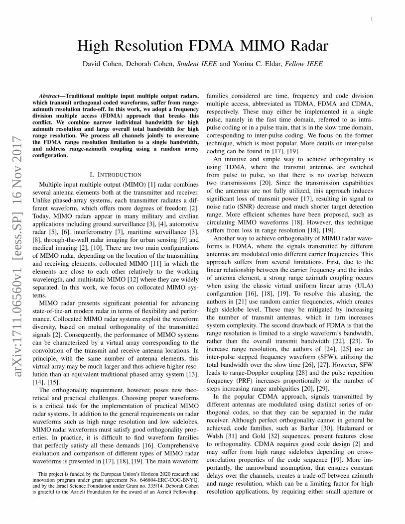
standard array structure and the corresponding virtual arrayare illustrated in Fig. 1 for R = 3 and T = 5. The circlesrepresent the receivers and the squares are the transmitters. Inour work, we will consider a random array configuration [38],where the antennas’ locations are chosen uniformly at randomwithin the aperture of the virtual array described above, thatis {ξm}M−1

m=0 ∼ U [0, Z] and {ζq}Q−1q=0 ∼ U [0, Z], respectively.

The corresponding virtual array has the same or a greateraperture than a traditional virtual array with the same numberof elements, depending on the locations of the antennas at thefar edges. The resulting azimuth resolution is thus at least asgood as that of the traditional virtual ULA structure.

3

Fig. 1. Illustration of MIMO arrays: (a) standard array, (b) correspondingreceiver virtual array.

Each transmitting antenna sends P pulses, such that the mthtransmitted signal is given by

sm(t) =

P−1∑p=0

hm (t− pτ)ej2πfct, 0 ≤ t ≤ Pτ, (1)

where hm (t) , 0 ≤ m ≤ T − 1 are orthogonal pulses withbandwidth Bh and modulated with carrier frequency fc. Thecoherent processing interval (CPI) is equal to Pτ , where τdenotes the pulse repetition interval (PRI). For convenience,we assume that fcτ is an integer, so that the initial phasefor every pulse e−j2πfcτp is canceled in the modulation for0 ≤ p ≤ P −1 [47]. The pulse time support is denoted by Tp,with 0 < Tp < τ .

MIMO radar architectures impose several requirements onthe transmitted waveform family. Besides traditional demandsfrom radar waveforms such as low sidelobes, MIMO transmitantennas rely on orthogonal waveforms. In addition, to avoidcross talk between the T signals and form TR channels, theorthogonality condition should be invariant to time shifts, thatis∫∞−∞ si (t) s∗j (t− τ0) dt = δ (i− j) , for i, j ∈ [0, T − 1]

and for all τ0. This property implies that the orthogonal signalscannot overlap in frequency (or time) [33], leading to theFDMA (or TDMA) approach. Alternatively, time invariantorthogonality can be approximately achieved using CDMA.

Both FDMA and CDMA follow the general model [48]:

hm(t) =

Nc∑u=1

wmuej2πfmutv(t− uδt), (2)

where each pulse is decomposed into Nc time slots withduration δt. Here, v(t) denotes the elementary waveform,wmu represents the code and fmu the frequency for the mthtransmission and uth time slot. The general expression (2)allows to analyze at the same time different waveform families.In particular, in CDMA, orthogonality is achieved by the code{wmu}Ncu=1 and fmu = 0 for all 1 ≤ u ≤ Nc. In FDMA,Nc = 1, wmu = 1 and δt = 0. The center frequenciesfmu = fm are chosen in [−TBh2 , TBh2 ] so that the intervals[fm− Bh

2 , fm+ Bh2 ] do not overlap. For simplicity of notation,

{hm(t)}T−1m=0 can be considered as frequency-shifted versions

of a low-pass pulse v(t) = h0(t) whose Fourier transformH0 (ω) has bandwidth Bh, such that

Hm (ω) = H0 (ω − 2πfm) . (3)

We adopt a unified notation for the total bandwidth Btot =TBh for FDMA and Btot = Bh for CDMA.

Consider L non-fluctuating point-targets, according to theSwerling-0 model [43]. Each target is identified by its pa-rameters: radar cross section (RCS) αl, distance between thetarget and the array origin or range Rl, velocity vl and azimuthangle relative to the array θl. Our goal is to recover the targets’delay τl = 2Rl

c , azimuth sine ϑl = sin(θl) and Doppler shiftfDl = 2vl

c fc from the received signals. In the sequel, we usethe terms range and delay interchangeably, as well as azimuthangle and sine, and velocity and Doppler frequency.

B. Received SignalThe transmitted pulses are reflected by the targets and

collected at the receive antennas. The following assumptionsare adopted on the array structure and targets’ location andmotion, leading to a simplified expression for the receivedsignal.A1 Collocated array - target RCS αl and θl are constant over

the array (see [49] for more details).A2 Far targets - target-radar distance is large compared to the

distance change during the CPI, which allows for constantαl,

vlPτ �cτl2. (4)

A3 Slow targets - low target velocity allows for constant τlduring the CPI,

2vlPτ

c� 1

Btot, (5)

and constant Doppler phase during pulse time Tp,

fDl Tp � 1. (6)

A4 Low acceleration - target velocity vl remains approxi-mately constant during the CPI, allowing for constantDoppler shift fDl ,

vlPτ �c

2fcPτ. (7)

A5 Narrowband waveform - small aperture allows τl to beconstant over the channels,

2Zλ

c� 1

Btot. (8)

Under assumptions A1, A2 and A4, the received signalxq(t) at the qth antenna is a sum of time-delayed, scaledreplica of the transmitted signals:

xq (t) =

P−1∑p−0

T−1∑m=0

L∑l=1

αlsm

(c− vlc+ vl

(t− Rl,mq

c− vl

)), (9)

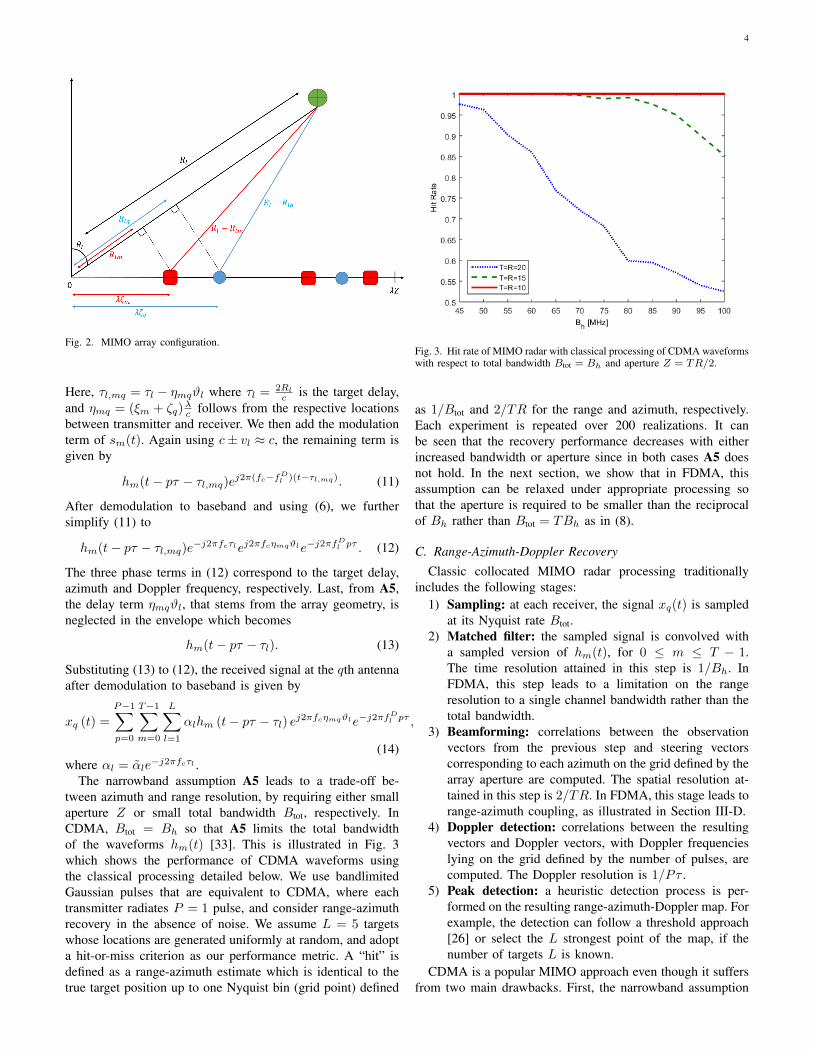
where Rl,mq = 2Rl − (Rlm + Rlq), with Rlm = λξmϑland Rlq = λζqϑl accounting for the array geometry, asillustrated in Fig. 2. The received signal can be simplifiedusing assumptions A3 and A5, as we now show.

We start with the envelope hm(t), and consider the pthframe and the lth target. From c ± vl ≈ c, and neglectingthe term 2vlt

c using (5), we obtain

hm

(c− vlc+ vl

(t− Rl,mq

c− vl

)− pτ

)= hm(t− pτ − τl,mq).

(10)

4

Fig. 2. MIMO array configuration.

Here, τl,mq = τl − ηmqϑl where τl = 2Rlc is the target delay,

and ηmq = (ξm + ζq)λc follows from the respective locations

between transmitter and receiver. We then add the modulationterm of sm(t). Again using c± vl ≈ c, the remaining term isgiven by

hm(t− pτ − τl,mq)ej2π(fc−fDl )(t−τl,mq). (11)

After demodulation to baseband and using (6), we furthersimplify (11) to

hm(t− pτ − τl,mq)e−j2πfcτlej2πfcηmqϑle−j2πfDl pτ . (12)

The three phase terms in (12) correspond to the target delay,azimuth and Doppler frequency, respectively. Last, from A5,the delay term ηmqϑl, that stems from the array geometry, isneglected in the envelope which becomes

hm(t− pτ − τl). (13)

Substituting (13) to (12), the received signal at the qth antennaafter demodulation to baseband is given by

xq (t) =

P−1∑p=0

T−1∑m=0

L∑l=1

αlhm (t− pτ − τl) ej2πfcηmqϑle−j2πfDl pτ ,

(14)where αl = αle

−j2πfcτl .The narrowband assumption A5 leads to a trade-off be-

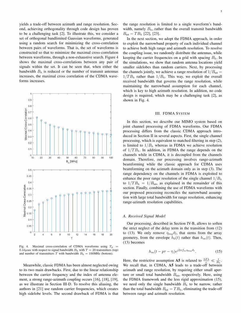
tween azimuth and range resolution, by requiring either smallaperture Z or small total bandwidth Btot, respectively. InCDMA, Btot = Bh so that A5 limits the total bandwidthof the waveforms hm(t) [33]. This is illustrated in Fig. 3which shows the performance of CDMA waveforms usingthe classical processing detailed below. We use bandlimitedGaussian pulses that are equivalent to CDMA, where eachtransmitter radiates P = 1 pulse, and consider range-azimuthrecovery in the absence of noise. We assume L = 5 targetswhose locations are generated uniformly at random, and adopta hit-or-miss criterion as our performance metric. A “hit” isdefined as a range-azimuth estimate which is identical to thetrue target position up to one Nyquist bin (grid point) defined

Fig. 3. Hit rate of MIMO radar with classical processing of CDMA waveformswith respect to total bandwidth Btot = Bh and aperture Z = TR/2.

as 1/Btot and 2/TR for the range and azimuth, respectively.Each experiment is repeated over 200 realizations. It canbe seen that the recovery performance decreases with eitherincreased bandwidth or aperture since in both cases A5 doesnot hold. In the next section, we show that in FDMA, thisassumption can be relaxed under appropriate processing sothat the aperture is required to be smaller than the reciprocalof Bh rather than Btot = TBh as in (8).

C. Range-Azimuth-Doppler RecoveryClassic collocated MIMO radar processing traditionally

includes the following stages:1) Sampling: at each receiver, the signal xq(t) is sampled

at its Nyquist rate Btot.2) Matched filter: the sampled signal is convolved with

a sampled version of hm(t), for 0 ≤ m ≤ T − 1.The time resolution attained in this step is 1/Bh. InFDMA, this step leads to a limitation on the rangeresolution to a single channel bandwidth rather than thetotal bandwidth.

3) Beamforming: correlations between the observationvectors from the previous step and steering vectorscorresponding to each azimuth on the grid defined by thearray aperture are computed. The spatial resolution at-tained in this step is 2/TR. In FDMA, this stage leads torange-azimuth coupling, as illustrated in Section III-D.

4) Doppler detection: correlations between the resultingvectors and Doppler vectors, with Doppler frequencieslying on the grid defined by the number of pulses, arecomputed. The Doppler resolution is 1/Pτ .

5) Peak detection: a heuristic detection process is per-formed on the resulting range-azimuth-Doppler map. Forexample, the detection can follow a threshold approach[26] or select the L strongest point of the map, if thenumber of targets L is known.

CDMA is a popular MIMO approach even though it suffersfrom two main drawbacks. First, the narrowband assumption

5

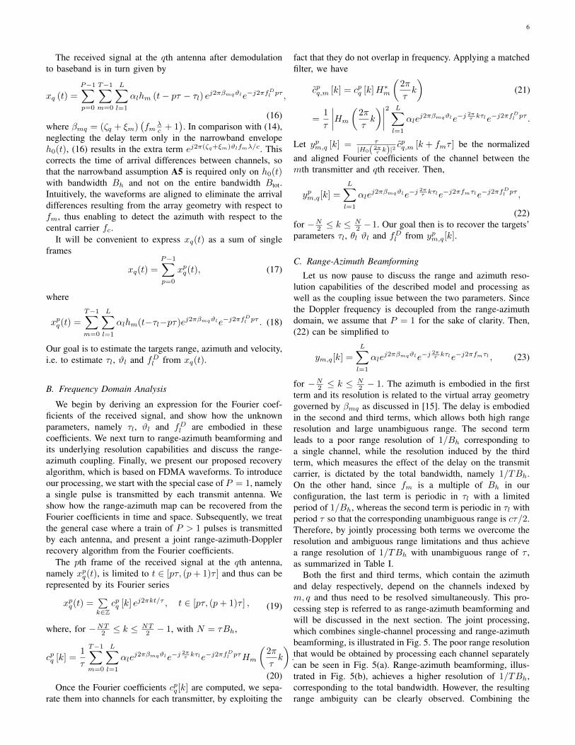
yields a trade-off between azimuth and range resolution. Sec-ond, achieving orthogonality through code design has provento be a challenging task [2]. To illustrate this, we consider aset of orthogonal bandlimited Gaussian waveforms, generatedusing a random search for minimizing the cross-correlationbetween pairs of waveforms. That is, the set of waveforms isconstructed so that to minimize the maximal cross-correlationbetween waveforms, through a non-exhaustive search. Figure 4shows the maximal cross-correlations between any pair ofsignals within the set. It can be seen that, when either thebandwidth Bh is reduced or the number of transmit antennasincreases, the maximal cross correlation of the CDMA wave-forms increases.

Fig. 4. Maximal cross-correlation of CDMA waveforms using Tp =0.44µsec with respect to signal bandwidth Bh with T = 20 transmitters (top)and number of transmitters T with bandwidth Bh = 100MHz (bottom).

Meanwhile, classic FDMA has been almost neglected owingto its two main drawbacks. First, due to the linear relationshipbetween the carrier frequency and the index of antenna ele-ment, a strong range-azimuth coupling occurs [16], [18], [19],as we illustrate in Section III-D. To resolve this aliasing, theauthors in [21] use random carrier frequencies, which createshigh sidelobe levels. The second drawback of FDMA is that

the range resolution is limited to a single waveform’s band-width, namely Bh, rather than the overall transmit bandwidthBtot = TBh [22], [23].

In the next section, we adopt the FDMA approach, in orderto exploit the narrowband property of each individual channelto achieve both high range and azimuth resolution. To resolvethe coupling issue, we randomly distribute the antennas, whilekeeping the carrier frequencies on a grid with spacing Bh. Inthe simulations, we show that random antenna locations yieldsmaller sidelobes than random carriers. Next, by processingthe channels jointly, we achieve a range resolution of 1/Btot =1/TBh rather than 1/Bh. This way, we exploit the overallreceived bandwidth that governs the range resolution, whilemaintaining the narrowband assumption for each channel,which is key to high azimuth resolution. In addition, no codedesign is required, which may be a challenging task [2], asshown in Fig. 4.

III. FDMA SYSTEM

In this section, we describe our MIMO system based onjoint channel processing of FDMA waveforms. Our FDMAprocessing differs from the classic CDMA approach intro-duced in Section II in several aspects. First, the single channelprocessing, which is equivalent to matched filtering in step (2),is limited to 1/Bh whereas in FDMA we achieve resolutionof 1/TBh. In addition, in FDMA the range depends on thechannels while in CDMA, it is decoupled from the channelsdomain. Therefore, our processing involves range-azimuthbeamforming while the classic approach for CDMA usesbeamforming on the azimuth domain only as in step (3). Therange dependency on the channels in FDMA is exploited toenhance the poor range resolution of the single channel 1/Bhto 1/TBh = 1/Btot, as explained in the remainder of thissection. Finally, combining the use of FDMA waveforms withour proposed processing reconciles the narrowband assump-tion with large total bandwidth for range resolution, enhancingrange-azimuth resolution capabilities.

A. Received Signal Model

Our processing, described in Section IV-B, allows to softenthe strict neglect of the delay term in the transition from (12)to (13). We only remove ηmqϑl, that stems from the arraygeometry, from the envelope h0(t) rather than hm(t). Then,(13) becomes

hm(t− pτ − τl)ej2πfmηmqϑl . (15)

Here, the restrictive assumption A5 is relaxed to 2Zλc �

1Bh

.We recall that, in CDMA, A5 leads to a trade-off betweenazimuth and range resolution, by requiring either small aper-ture or small total bandwidth Btot, respectively. Here, usingthe FDMA framework and the less rigid approximation (15),we need only the single bandwidth Bh to be narrow, ratherthan the total bandwidth Btot = TBh, eliminating the trade-offbetween range and azimuth resolution.

6

The received signal at the qth antenna after demodulationto baseband is in turn given by

xq (t) =

P−1∑p=0

T−1∑m=0

L∑l=1

αlhm (t− pτ − τl) ej2πβmqϑle−j2πfDl pτ ,

(16)where βmq = (ζq + ξm)

(fm

λc + 1

). In comparison with (14),

neglecting the delay term only in the narrowband envelopeh0(t), (16) results in the extra term ej2π(ζq+ξm)ϑlfmλ/c. Thiscorrects the time of arrival differences between channels, sothat the narrowband assumption A5 is required only on h0(t)with bandwidth Bh and not on the entire bandwidth Btot.Intuitively, the waveforms are aligned to eliminate the arrivaldifferences resulting from the array geometry with respect tofm, thus enabling to detect the azimuth with respect to thecentral carrier fc.

It will be convenient to express xq(t) as a sum of singleframes

xq(t) =

P−1∑p=0

xpq(t), (17)

where

xpq(t) =

T−1∑m=0

L∑l=1

αlhm(t−τl−pτ)ej2πβmqϑle−j2πfDl pτ . (18)

Our goal is to estimate the targets range, azimuth and velocity,i.e. to estimate τl, ϑl and fDl from xq(t).

B. Frequency Domain Analysis

We begin by deriving an expression for the Fourier coef-ficients of the received signal, and show how the unknownparameters, namely τl, ϑl and fDl are embodied in thesecoefficients. We next turn to range-azimuth beamforming andits underlying resolution capabilities and discuss the range-azimuth coupling. Finally, we present our proposed recoveryalgorithm, which is based on FDMA waveforms. To introduceour processing, we start with the special case of P = 1, namelya single pulse is transmitted by each transmit antenna. Weshow how the range-azimuth map can be recovered from theFourier coefficients in time and space. Subsequently, we treatthe general case where a train of P > 1 pulses is transmittedby each antenna, and present a joint range-azimuth-Dopplerrecovery algorithm from the Fourier coefficients.

The pth frame of the received signal at the qth antenna,namely xpq(t), is limited to t ∈ [pτ, (p+ 1)τ ] and thus can berepresented by its Fourier series

xpq(t) =∑k∈Z

cpq [k] ej2πkt/τ , t ∈ [pτ, (p+ 1)τ ] , (19)

where, for −NT2 ≤ k ≤NT2 − 1, with N = τBh,

cpq [k] =1

τ

T−1∑m=0

L∑l=1

αlej2πβmqϑle−j

2πτ kτle−j2πf

Dl pτHm

(2π

τk

).

(20)Once the Fourier coefficients cpq [k] are computed, we sepa-

rate them into channels for each transmitter, by exploiting the

fact that they do not overlap in frequency. Applying a matchedfilter, we have

cpq,m [k] = cpq [k]H∗m

(2π

τk

)(21)

=1

τ

∣∣∣∣Hm

(2π

τk

)∣∣∣∣2 L∑l=1

αlej2πβmqϑle−j

2πτ kτle−j2πf

Dl pτ .

Let ypm,q [k] = τ

|H0( 2πτ k)|2

cpq,m [k + fmτ ] be the normalizedand aligned Fourier coefficients of the channel between themth transmitter and qth receiver. Then,

ypm,q[k] =

L∑l=1

αlej2πβmqϑle−j

2πτ kτle−j2πfmτle−j2πf

Dl pτ ,

(22)for −N2 ≤ k ≤

N2 −1. Our goal then is to recover the targets’

parameters τl, θl ϑl and fDl from ypm,q[k].

C. Range-Azimuth Beamforming

Let us now pause to discuss the range and azimuth reso-lution capabilities of the described model and processing aswell as the coupling issue between the two parameters. Sincethe Doppler frequency is decoupled from the range-azimuthdomain, we assume that P = 1 for the sake of clarity. Then,(22) can be simplified to

ym,q[k] =

L∑l=1

αlej2πβmqϑle−j

2πτ kτle−j2πfmτl , (23)

for −N2 ≤ k ≤ N2 − 1. The azimuth is embodied in the first

term and its resolution is related to the virtual array geometrygoverned by βmq as discussed in [15]. The delay is embodiedin the second and third terms, which allows both high rangeresolution and large unambiguous range. The second termleads to a poor range resolution of 1/Bh corresponding toa single channel, while the resolution induced by the thirdterm, which measures the effect of the delay on the transmitcarrier, is dictated by the total bandwidth, namely 1/TBh.On the other hand, since fm is a multiple of Bh in ourconfiguration, the last term is periodic in τl with a limitedperiod of 1/Bh, whereas the second term is periodic in τl withperiod τ so that the corresponding unambiguous range is cτ/2.Therefore, by jointly processing both terms we overcome theresolution and ambiguous range limitations and thus achievea range resolution of 1/TBh with unambiguous range of τ ,as summarized in Table I.

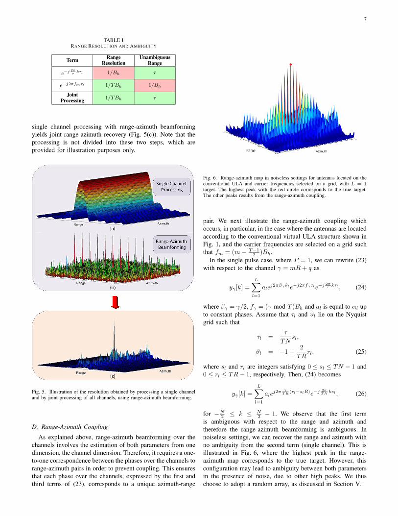
Both the first and third terms, which contain the azimuthand delay respectively, depend on the channels indexed bym, q and thus need to be resolved simultaneously. This pro-cessing step is referred to as range-azimuth beamforming andwill be discussed in the next section. The joint processing,which combines single-channel processing and range-azimuthbeamforming, is illustrated in Fig. 5. The poor range resolutionthat would be obtained by processing each channel separatelycan be seen in Fig. 5(a). Range-azimuth beamforming, illus-trated in Fig. 5(b), achieves a higher resolution of 1/TBh,corresponding to the total bandwidth. However, the resultingrange ambiguity can be clearly observed. Combining the

7

TABLE IRANGE RESOLUTION AND AMBIGUITY

Term RangeResolution

UnambiguousRange

e−j2πτkτl 1/Bh τ

e−j2πfmτl 1/TBh 1/Bh

JointProcessing 1/TBh τ

single channel processing with range-azimuth beamformingyields joint range-azimuth recovery (Fig. 5(c)). Note that theprocessing is not divided into these two steps, which areprovided for illustration purposes only.

Fig. 5. Illustration of the resolution obtained by processing a single channeland by joint processing of all channels, using range-azimuth beamforming.

D. Range-Azimuth Coupling

As explained above, range-azimuth beamforming over thechannels involves the estimation of both parameters from onedimension, the channel dimension. Therefore, it requires a one-to-one correspondence between the phases over the channels torange-azimuth pairs in order to prevent coupling. This ensuresthat each phase over the channels, expressed by the first andthird terms of (23), corresponds to a unique azimuth-range

Fig. 6. Range-azimuth map in noiseless settings for antennas located on theconventional ULA and carrier frequencies selected on a grid, with L = 1target. The highest peak with the red circle corresponds to the true target.The other peaks results from the range-azimuth coupling.

pair. We next illustrate the range-azimuth coupling whichoccurs, in particular, in the case where the antennas are locatedaccording to the conventional virtual ULA structure shown inFig. 1, and the carrier frequencies are selected on a grid suchthat fm = (m− T−1

2 )Bh.In the single pulse case, where P = 1, we can rewrite (23)

with respect to the channel γ = mR+ q as

yγ [k] =

L∑l=1

alej2πβγϑle−j2πfγτle−j

2πτ kτl , (24)

where βγ = γ/2, fγ = (γ mod T )Bh and al is equal to αl upto constant phases. Assume that τl and ϑl lie on the Nyquistgrid such that

τl =τ

TNsl,

ϑl = −1 +2

TRrl, (25)

where sl and rl are integers satisfying 0 ≤ sl ≤ TN − 1 and0 ≤ rl ≤ TR− 1, respectively. Then, (24) becomes

yγ [k] =

L∑l=1

alej2π γ

TR (rl−slR)e−j2πTN ksl , (26)

for −N2 ≤ k ≤ N2 − 1. We observe that the first term

is ambiguous with respect to the range and azimuth andtherefore the range-azimuth beamforming is ambiguous. Innoiseless settings, we can recover the range and azimuth withno ambiguity from the second term (single channel). This isillustrated in Fig. 6, where the highest peak in the range-azimuth map corresponds to the true target. However, thisconfiguration may lead to ambiguity between both parametersin the presence of noise, due to other high peaks. We thuschoose to adopt a random array, as discussed in Section V.

8

IV. RANGE-AZIMUTH-DOPPLER RECOVERY

We now describe our recovery approach from the Fouriercoefficients of the FDMA received waveforms (16). We firstconsider the case where P = 1 and derive range-azimuthrecovery from the coefficients (23). We next turn to range-azimuth-Doppler recovery from (22).

A. Range-Azimuth Recovery

In practice, as in traditional MIMO, suppose we nowlimit ourselves to the Nyquist grid with respect to the totalbandwidth TBh so that τl and ϑl lie on the grid defined in(25). Let Ym be the N ×R matrix with qth column given byym,q[k −N/2], defined in (23), for 0 ≤ k ≤ N − 1. We canwrite Ym as

Ym = AmX (Bm)T. (27)

Here, Am denotes the N×TN matrix whose (k, n)th elementis e−j

2πTN (k−N2 )ne

−j2π fmBhnT and Bm is the R × TR matrix

with (q, p)th element ej2πβmq(−1+ 2TRp). The matrix X is a

TN × TR sparse matrix that contains the values αl at the Lindices (sl, rl).

Our goal is to recover X from the measurement matricesYm, 0 ≤ m ≤M−1. The time and spatial resolution inducedby X are τ

TN = 1TBh

, and 2TR , respectively, as in classic

CDMA processing.Define

A = [A0T A1T · · · A(T−1)T ]T , (28)

andB = [B0T B1T · · · B(T−1)T ]T . (29)

To better grasp the structure of A and B, suppose that thecarriers fm lie on the grid fm = (m− T−1

2 )Bh. In this case,the (k, n)th element of Am is e−j

2πTN (k+mN−TN2 )n and A is

the TN×TN Fourier matrix up to row permutation. Similarly,assuming that the antenna elements lie on the virtual arrayillustrated in Fig. 1, we have βmq = 1

2 (q + mR), wherewe used A5 to simplify the expression. Then, the (q, p)thelement of Bm is ej

2πTR (q+mR)(p−TR2 ) and B is the TR×TR

Fourier matrix up to column permutation. The matrices A andB are sometimes referred to as dictionaries, whose columnscorrespond to the range and azimuth grid points, respectively.However, this configuration leads to range-azimuth couplingas discussed in Section III-D. In Section V, we use a randomarray to avoid range-azimuth coupling.

One approach to solving (27) is based on CS [50], [39]techniques that exploits the sparsity of the target scene. One ofCS recovery advantages is that it allows to reduce the numberof required samples, pulses and channels while preserving theunderlying resolution [51]. In particular, we adopt an itera-tive reconstruction approach that is beneficial when dealingwith high dynamic range with both weak and strong targets,especially since the sidelobes are slightly raised due to therandom array configuration. Our recovery algorithm is basedon orthogonal matching pursuit (OMP) [50], [39]. Similarsubtraction techniques are used in many iterative algorithmssuch as the CLEAN process [52].

To recover the sparse matrix X from the set of equations(27), for all 0 ≤ m ≤ M − 1, where the targets’ range andazimuth lie on the Nyquist grid, we consider the followingoptimization problem

min ||X||0 s.t. AmX (Bm)T

= Ym, 0 ≤ m ≤ T − 1.(30)

It has been shown in [51] that the minimal number of channelsrequired for perfect recovery of X in (30) with L targets innoiseless settings is TR ≥ 2L with a minimal number ofTN ≥ 2L samples per receiver. To solve (30), we extend thematrix OMP from [53] to simultaneously solve a system ofCS matrix equations, as shown in Algorithm 1. In the algo-rithm description, vec(Y) ,

[vec(Y0)T · · · vec(YT−1)T

]T,

dt(l) =[(d0t (l))

T · · · (dT−1t (l))T

]Twhere dmt (l) =

vec(amΛt(l,1)(bmΛt(l,2))

T ) with Λt(l, i) the (l, i)th element in theindex set Λt at the tth iteration, and Dt = [dt(1) . . . dt(t)].Here, amj denotes the jth column of the matrix Am andbmj denotes the jth column of the matrix Bm. Once X isrecovered, the delays and azimuths are estimated as

τl =τ

TNΛL(l, 1), (31)

ϑl = −1 +2

TRΛL(l, 2). (32)

Other CS recovery algorithms, such as FISTA [54], [55], can

Algorithm 1 Simultaneous sparse 2D recovery based OMPInput: Observation matrices Ym, measurement matrices

Am, Bm, for all 0 ≤ m ≤ T − 1Output: Index set Λ containing the locations of the non zero

indices of X, estimate for sparse matrix X1: Initialization: residual Rm

0 = Ym, index set Λ0 = ∅,t = 1

2: Project residual onto measurement matrices:

Ψ = AHRB

where A and B are defined in (28) and (29), respectively,and R = diag

([R0

t−1 · · · RT−1t−1 ]

)is block diagonal

3: Find the two indices λt = [λt(1) λt(2)] such that

[λt(1) λt(2)] = arg maxi,j |Ψi,j |

4: Augment index set Λt = Λt⋃{λt}

5: Find the new signal estimate

α = [α1 . . . αt]T = (DT

t Dt)−1DT

t vec(Y)

6: Compute new residual

Rmt = Rm

0 −t∑l=1

αlamΛt(l,1)

(bmΛt(l,2)

)T7: If t < L, increment t and return to step 2, otherwise stop8: Estimated support set Λ = ΛL9: Estimated matrix X: (ΛL(l, 1),ΛL(l, 2))-th component of

X is given by αl for l = 1, · · · , L while rest of theelements are zero

also be extended to our setting.

9

The projection performed in step 2 of the algorithm com-bines single channel processing with range-azimuth beam-forming. The former coherently processes the second termof (23), which appears in the matrix A, while range-azimuthbeamforming over the channels coherently processes the firstand third terms of (23), which are contained in A and B, re-spectively. The FDMA narrowband assumption reconciliationis due to the additional third term of (15), contained in B,thus enhancing range-azimuth resolution capabilities.

The improved performance of the iterative approach overnon-iterative target recovery with high dynamic range is illus-trated in simulations in Section V. There, we also compareour FDMA approach with classic CDMA, when using a non-iterative recovery method in the former. In particular, we onlyuse one iteration of Algorithm 1, which is equivalent to theclassic approach. This demonstrates that our FDMA methodoutperforms CDMA due to the high range-azimuth resolu-tion capabilities stemming from the reconciliation betweenthe individual narrowband assumption and the large overallbandwidth.

B. Range-Azimuth-Doppler Recovery

Besides τl and ϑl lying on the grid defined in (25), weassume that the Doppler frequency fDl is limited to theNyquist grid as well, defined by the CPI as:

fDl = − 1

2τ+

1

Pτul, (33)

where ul is an integer satisfying 0 ≤ ul ≤ P − 1. Let Zm

be the NR× P matrix with qth column given by the verticalconcatenation of ypm,q[k], such that the (k+ qN, p)th elementof Zm is given by (Zm)(k+qN,p) = ypm,q[k−N/2], defined in(22), for 0 ≤ k ≤ N − 1 and 0 ≤ q ≤ R − 1. We can thenwrite Zm as

Zm = (Bm ⊗Am) XDFT , (34)

where the N × TN matrix Am and the R× TR matrix Bm

are defined as in Section IV-A and F denotes the P × PFourier matrix up to column permutation. The matrix XD isa T 2NR× P sparse matrix that contains the values αl at theL indices (rlTN + sl, ul).

Our goal is now to recover XD from the measurementmatrices Zm, 0 ≤ m ≤ T −1. The time, spatial and frequencyresolution stipulated by XD are τ

TN = 1Btot

with Btot = TBh,2TR and 1

Pτ respectively, as in classic CDMA processing.To jointly recover the range, azimuth and Doppler frequency

of the targets, we apply the concept of Doppler focusingfrom [56] to our setting. Once the Fourier coefficients (22)are processed, we perform Doppler focusing for a specificfrequency ν, that is

Φνm,q[k] =

P−1∑p=0

ypm,q[k]ej2πνpτ (35)

=

L∑l=1

αlej2πβmqϑle−j

2πτ (k+fmτ)τl

P−1∑p=0

ej2π(ν−fDl )pτ ,

for −N2 ≤ k ≤ −N2 − 1. Following the same argument as in[56], it holds that

P−1∑p=0

ej2π(ν−fDl )pτ ∼={P |ν − fDl | < 1

2Pτ ,0 otherwise. (36)

Therefore, for each focused frequency ν, (35) reduces to a 2-dimensional problem. We note that Doppler focusing increasesthe SNR by a factor a P , as can be seen in (36).

Algorithm 2 solves (34) for 0 ≤ m ≤ T − 1 usingDoppler focusing. Note that step 1 can be performed usingthe fast Fourier transform (FFT). In the algorithm descrip-tion, vec(Z) is defined as in the previous section, et(l) =[(e0t (l))

T · · · (eT−1t (l))T

]Twhere emt (l) = vec((Bm ⊗

Am)Λt(l,2)TN+Λt(l,1)(FmΛt(l,3))

T ) with Λt(l, i) the (l, i)th el-ement in the index set Λt at the tth iteration, and Et =[et(1) . . . et(t)]. Once XD is recovered, the delays and az-imuths are given by (31) and (32), respectively, and theDoppler frequencies are estimated as

fDl = − 1

2τ+

ΛL(l, 3)

Pτ. (37)

Similarly to the one-pulse case, the minimal number of chan-nels required for perfect recovery of XD with L targets innoiseless settings is TR ≥ 2L with a minimal number ofTN ≥ 2L samples per receiver and P ≥ 2L pulses pertransmitter [51].

V. SIMULATIONS

In this section, we present numerical experiments illustrat-ing our FDMA approach and compare our method with classicMIMO processing using CDMA.

A. Preliminaries

Throughout the experiments, the standard MIMO systemis based on a virtual array, as depicted in Fig. 1 generatedby T = 20 transmit antennas and R = 20 receive antennas,yielding an aperture λZ = 6m. We consider a random arrayconfiguration where the transmitters and receivers’ locationsare selected uniformly at random over the aperture Z. We useFDMA waveforms hm(t) such that fm = (im − T−1

2 )Bh,where im are integers chosen uniformly at random in [0, T ),for 0 ≤ m ≤ T − 1, and all frequency bands within[−T2Bh,

T2Bh] are used for transmission. We consider the

following parameters: PRI τ = 100µsec, bandwidth Bh =5MHz and carrier frequency fc = 10GHz. We simulatetargets from the Swerling-0 model with identical amplitudesand random phases. The received signals are corrupted byuncorrelated additive Gaussian noise (AWGN) with powerspectral density N0. The SNR is defined as

SNR =

1Tp

∫ Tp0|h0(t)|2dt

N0Bh, (38)

where Tp is the pulse time.We consider a hit-or-miss criterion as performance metric. A

“hit” is defined as a range-azimuth estimate which is identicalto the true target position up to one Nyquist bin (grid point)

10

Algorithm 2 Simultaneous sparse 3D recovery based OMPwith focusingInput: Observation matrices Zm, measurement matrices

Am, Bm, for all 0 ≤ m ≤ T − 1Output: Index set Λ containing the locations of the non zero

indices of XD, estimate for sparse matrix XD

1: Perform Doppler focusing for 0 ≤ i ≤ N − 1, 0 ≤ j ≤R− 1 and 0 ≤ ν ≤ P − 1 :

Φ(m,ν)i,j = (ZmF)i+jN,ν .

2: Initialization: residual R(m,ν)0 = Φ(m,ν), index set Λ0 =

∅, t = 13: Project residual onto measurement matrices for 0 ≤ ν ≤P − 1:

Ψν = AHRνB,

where A and B are defined in (28) and (29), respectively,and Rν = diag

([R

(0,ν)t−1 · · · R

(T−1,ν)t−1 ]

)is block diagonal

4: Find the three indices λt = [λt(1)λt(2)λt(3)] such that

[λt(1) λt(2) λt(3)] = arg maxi,j,ν∣∣Ψν

i,j

∣∣5: Augment index set Λt = Λt

⋃{λt}

6: Find the new signal estimate

α = [α1 . . . αt]T = (ET

t Et)−1ET

t vec(Z)

7: Compute new residual

R(m,ν)t = R

(m,ν)0 −

t∑l=1

αlamΛt(l,1)

(bmΛt(l,2)

)T (fΛt(l,3)

)Tfν

8: If t < L, increment t and return to step 3, otherwise stop9: Estimated support set Λ = ΛL

10: Estimated matrix XD:(ΛL(l, 2)TN + ΛL(l, 1),ΛL(l, 3))-th component ofXD is given by αl for l = 1, · · · , L while rest of theelements are zero

defined as 1/TBh and 2/TR for the range and azimuth,respectively. In pulse-Doppler settings, a “hit” is proclaimed ifthe recovered Doppler is identical to the true frequency up toone Nyquist bin of size 1/Pτ , in addition to the two previousconditions.

B. Numerical Results

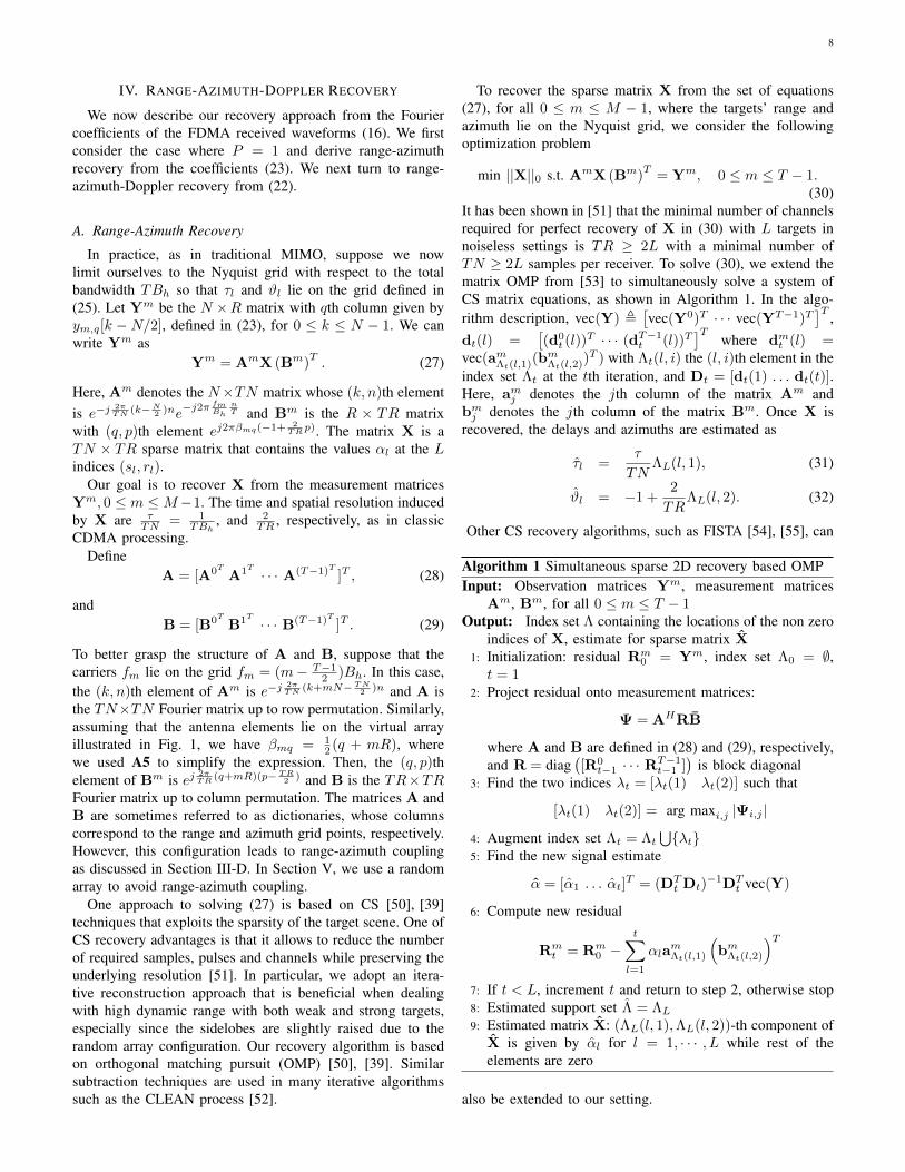
We first consider a sparse target scene with L = 6 targetsincluding a couple of targets with close ranges, a couplewith close azimuths and another couple with close velocities.We use P = 10 pulses and the SNR is set to −10dB. Ascan be seen in Fig. 7, all targets are perfectly recovered,demonstrating high resolution in all dimensions. Here, therange and azimuth are converted to 2-dimensional x and ylocations.

We next turn to the range-azimuth coupling issue and dis-cuss the impact of the choice of antennas’ locations and trans-missions’ carrier frequencies. As discussed in Section III-D,the conventional ULA array structure shown in Fig. 1 withcarrier frequency selected on a grid, leads to ambiguity in

Fig. 7. Range-azimuth-Doppler recovery for L = 6 targets and SNR=−10dB.

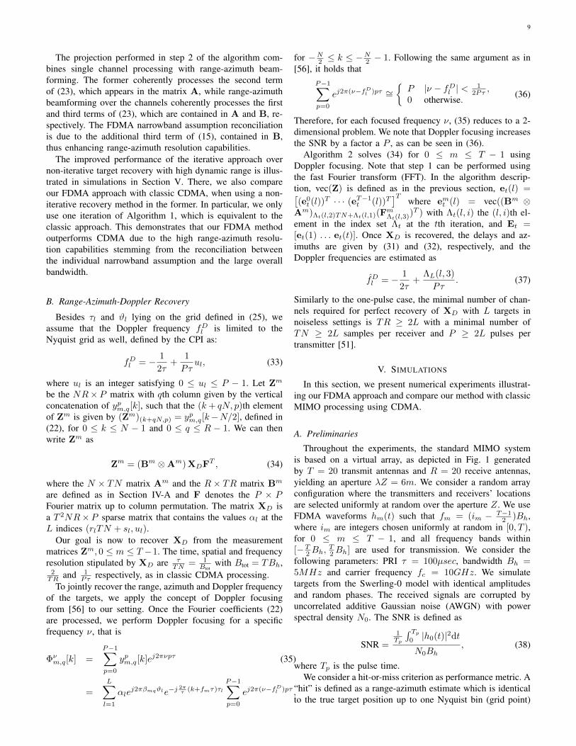
Fig. 8. Range-azimuth map in noiseless settings for random carrier frequen-cies along range axis (a) and azimuth axis (b), and for random antennas’locations along range axis (c) and azimuth axis (d), for L = 1 target. Thered dotted line indicates the peak sidelobe level for this target.

the range-azimuth domain. In order to overcome the ambi-guity issue, we adopt a random array configuration [38]. Wefound heuristically that a configuration with random antennas’locations with carriers on a grid provides better results thanrandom carriers with a ULA structure. Figure 8 shows a typicalresult of sidelobes for both configurations. The peak sidelobelevel for the configuration with random antennas’ locations isconsistently lower.

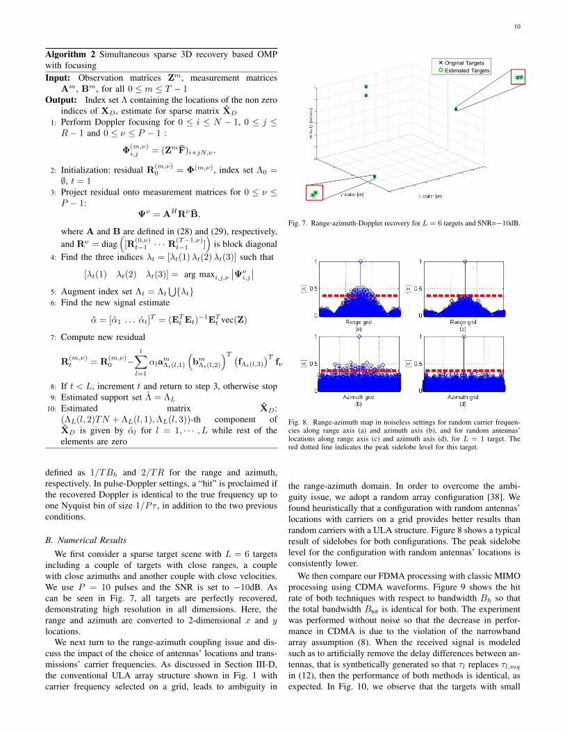
We then compare our FDMA processing with classic MIMOprocessing using CDMA waveforms. Figure 9 shows the hitrate of both techniques with respect to bandwidth Bh so thatthe total bandwidth Btot is identical for both. The experimentwas performed without noise so that the decrease in perfor-mance in CDMA is due to the violation of the narrowbandarray assumption (8). When the received signal is modeledsuch as to artificially remove the delay differences between an-tennas, that is synthetically generated so that τl replaces τl,mqin (12), then the performance of both methods is identical, asexpected. In Fig. 10, we observe that the targets with small

11

Fig. 9. Hit rate of FDMA and classic CDMA versus bandwidth.

Fig. 10. Range-azimuth recovery for L = 4 targets using classic CDMA (a)and FDMA (b) .

azimuth angle θl are detected by both techniques, whereastargets on the end-fire direction (θl = ±90◦, corresponds tothe broadside direction) are missed by the CDMA approach.This happens because the delay differences between channelsare too large, which violates the narrowband assumption A5.

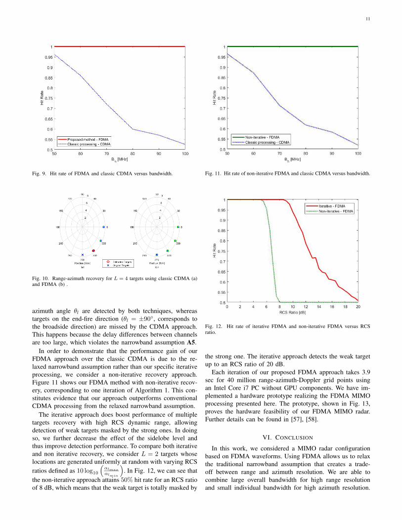
In order to demonstrate that the performance gain of ourFDMA approach over the classic CDMA is due to the re-laxed narrowband assumption rather than our specific iterativeprocessing, we consider a non-iterative recovery approach.Figure 11 shows our FDMA method with non-iterative recov-ery, corresponding to one iteration of Algorithm 1. This con-stitutes evidence that our approach outperforms conventionalCDMA processing from the relaxed narrowband assumption.

The iterative approach does boost performance of multipletargets recovery with high RCS dynamic range, allowingdetection of weak targets masked by the strong ones. In doingso, we further decrease the effect of the sidelobe level andthus improve detection performance. To compare both iterativeand non iterative recovery, we consider L = 2 targets whoselocations are generated uniformly at random with varying RCSratios defined as 10 log10

(αlmaxαlmin

). In Fig. 12, we can see that

the non-iterative approach attains 50% hit rate for an RCS ratioof 8 dB, which means that the weak target is totally masked by

Fig. 11. Hit rate of non-iterative FDMA and classic CDMA versus bandwidth.

Fig. 12. Hit rate of iterative FDMA and non-iterative FDMA versus RCSratio.

the strong one. The iterative approach detects the weak targetup to an RCS ratio of 20 dB.

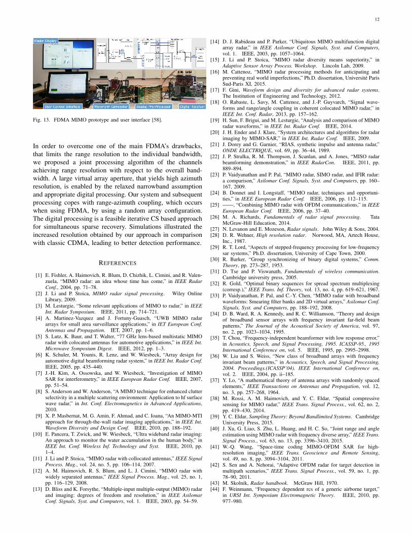
Each iteration of our proposed FDMA approach takes 3.9sec for 40 million range-azimuth-Doppler grid points usingan Intel Core i7 PC without GPU components. We have im-plemented a hardware prototype realizing the FDMA MIMOprocessing presented here. The prototype, shown in Fig. 13,proves the hardware feasibility of our FDMA MIMO radar.Further details can be found in [57], [58].

VI. CONCLUSION

In this work, we considered a MIMO radar configurationbased on FDMA waveforms. Using FDMA allows us to relaxthe traditional narrowband assumption that creates a trade-off between range and azimuth resolution. We are able tocombine large overall bandwidth for high range resolutionand small individual bandwidth for high azimuth resolution.

12

Fig. 13. FDMA MIMO prototype and user interface [58].

In order to overcome one of the main FDMA’s drawbacks,that limits the range resolution to the individual bandwidth,we proposed a joint processing algorithm of the channelsachieving range resolution with respect to the overall band-width. A large virtual array aperture, that yields high azimuthresolution, is enabled by the relaxed narrowband assumptionand appropriate digital processing. Our system and subsequentprocessing copes with range-azimuth coupling, which occurswhen using FDMA, by using a random array configuration.The digital processing is a feasible iterative CS based approachfor simultaneous sparse recovery. Simulations illustrated theincreased resolution obtained by our approach in comparisonwith classic CDMA, leading to better detection performance.

REFERENCES

[1] E. Fishler, A. Haimovich, R. Blum, D. Chizhik, L. Cimini, and R. Valen-zuela, “MIMO radar: an idea whose time has come,” in IEEE RadarConf., 2004, pp. 71–78.

[2] J. Li and P. Stoica, MIMO radar signal processing. Wiley OnlineLibrary, 2009.

[3] M. Lesturgie, “Some relevant applications of MIMO to radar,” in IEEEInt. Radar Symposium. IEEE, 2011, pp. 714–721.

[4] A. Martinez-Vazquez and J. Fortuny-Guasch, “UWB MIMO radararrays for small area surveillance applications,” in IET European Conf.Antennas and Propagation. IET, 2007, pp. 1–6.

[5] S. Lutz, K. Baur, and T. Walter, “77 GHz lens-based multistatic MIMOradar with colocated antennas for automotive applications,” in IEEE Int.Microwave Symposium Digest. IEEE, 2012, pp. 1–3.

[6] K. Schuler, M. Younis, R. Lenz, and W. Wiesbeck, “Array design forautomotive digital beamforming radar system,” in IEEE Int. Radar Conf.IEEE, 2005, pp. 435–440.

[7] J.-H. Kim, A. Ossowska, and W. Wiesbeck, “Investigation of MIMOSAR for interferometry,” in IEEE European Radar Conf. IEEE, 2007,pp. 51–54.

[8] S. Anderson and W. Anderson, “A MIMO technique for enhanced clutterselectivity in a multiple scattering environment: Application to hf surfacewave radar,” in Int. Conf. Electromagnetics in Advanced Applications,2010.

[9] X. P. Masbernat, M. G. Amin, F. Ahmad, and C. Ioana, “An MIMO-MTIapproach for through-the-wall radar imaging applications,” in IEEE Int.Waveform Diversity and Design Conf. IEEE, 2010, pp. 188–192.

[10] E. Pancera, T. Zwick, and W. Wiesbeck, “Ultra wideband radar imaging:An approach to monitor the water accumulation in the human body,” inIEEE Int. Conf. Wireless Inf. Technology and Syst. IEEE, 2010, pp.1–4.

[11] J. Li and P. Stoica, “MIMO radar with collocated antennas,” IEEE SignalProcess. Mag., vol. 24, no. 5, pp. 106–114, 2007.

[12] A. M. Haimovich, R. S. Blum, and L. J. Cimini, “MIMO radar withwidely separated antennas,” IEEE Signal Process. Mag., vol. 25, no. 1,pp. 116–129, 2008.

[13] D. Bliss and K. Forsythe, “Multiple-input multiple-output (MIMO) radarand imaging: degrees of freedom and resolution,” in IEEE AsilomarConf. Signals, Syst. and Computers, vol. 1. IEEE, 2003, pp. 54–59.

[14] D. J. Rabideau and P. Parker, “Ubiquitous MIMO multifunction digitalarray radar,” in IEEE Asilomar Conf. Signals, Syst. and Computers,vol. 1. IEEE, 2003, pp. 1057–1064.

[15] J. Li and P. Stoica, “MIMO radar diversity means superiority,” inAdaptive Sensor Array Process. Workshop. Lincoln Lab, 2009.

[16] M. Cattenoz, “MIMO radar processing methods for anticipating andpreventing real world imperfections,” Ph.D. dissertation, Universite ParisSud-Paris XI, 2015.

[17] F. Gini, Waveform design and diversity for advanced radar systems.The Institution of Engineering and Technology, 2012.

[18] O. Rabaste, L. Savy, M. Cattenoz, and J.-P. Guyvarch, “Signal wave-forms and range/angle coupling in coherent colocated MIMO radar,” inIEEE Int. Conf. Radar, 2013, pp. 157–162.

[19] H. Sun, F. Brigui, and M. Lesturgie, “Analysis and comparison of MIMOradar waveforms,” in IEEE Int. Radar Conf. IEEE, 2014.

[20] J. H. Ender and J. Klare, “System architectures and algorithms for radarimaging by MIMO-SAR,” in IEEE Int. Radar Conf. IEEE, 2009.

[21] J. Dorey and G. Garnier, “RIAS, synthetic impulse and antenna radar,”ONDE ELECTRIQUE, vol. 69, pp. 36–44, 1989.

[22] J. P. Stralka, R. M. Thompson, J. Scanlan, and A. Jones, “MISO radarbeamforming demonstration,” in IEEE RadarCon. IEEE, 2011, pp.889–894.

[23] P. Vaidyanathan and P. Pal, “MIMO radar, SIMO radar, and IFIR radar:a comparison,” Asilomar Conf. Signals, Syst. and Computers, pp. 160–167, 2009.

[24] B. Donnet and I. Longstaff, “MIMO radar, techniques and opportuni-ties,” in IEEE European Radar Conf. IEEE, 2006, pp. 112–115.

[25] ——, “Combining MIMO radar with OFDM communications,” in IEEEEuropean Radar Conf. IEEE, 2006, pp. 37–40.

[26] M. A. Richards, Fundamentals of radar signal processing. TataMcGraw-Hill Education, 2014.

[27] N. Levanon and E. Mozeson, Radar signals. John Wiley & Sons, 2004.[28] D. R. Wehner, High resolution radar. Norwood, MA, Artech House,

Inc., 1987.[29] R. T. Lord, “Aspects of stepped-frequency processing for low-frequency

sar systems,” Ph.D. dissertation, University of Cape Town, 2000.[30] R. Barker, “Group synchronizing of binary digital systems,” Comm.

Theory, pp. 273–287, 1953.[31] D. Tse and P. Viswanath, Fundamentals of wireless communication.

Cambridge university press, 2005.[32] R. Gold, “Optimal binary sequences for spread spectrum multiplexing

(corresp.),” IEEE Trans. Inf. Theory, vol. 13, no. 4, pp. 619–621, 1967.[33] P. Vaidyanathan, P. Pal, and C.-Y. Chen, “MIMO radar with broadband

waveforms: Smearing filter banks and 2D virtual arrays,” Asilomar Conf.Signals, Syst. and Computers, pp. 188–192, 2008.

[34] D. B. Ward, R. A. Kennedy, and R. C. Williamson, “Theory and designof broadband sensor arrays with frequency invariant far-field beampatterns,” The Journal of the Acoustical Society of America, vol. 97,no. 2, pp. 1023–1034, 1995.

[35] T. Chou, “Frequency-independent beamformer with low response error,”in Acoustics, Speech, and Signal Processing, 1995. ICASSP-95., 1995International Conference on, vol. 5. IEEE, 1995, pp. 2995–2998.

[36] W. Liu and S. Weiss, “New class of broadband arrays with frequencyinvariant beam patterns,” in Acoustics, Speech, and Signal Processing,2004. Proceedings.(ICASSP’04). IEEE International Conference on,vol. 2. IEEE, 2004, pp. ii–185.

[37] Y. Lo, “A mathematical theory of antenna arrays with randomly spacedelements,” IEEE Transactions on Antennas and Propagation, vol. 12,no. 3, pp. 257–268, 1964.

[38] M. Rossi, A. M. Haimovich, and Y. C. Eldar, “Spatial compressivesensing for MIMO radar,” IEEE Trans. Signal Process., vol. 62, no. 2,pp. 419–430, 2014.

[39] Y. C. Eldar, Sampling Theory: Beyond Bandlimited Systems. CambridgeUniversity Press, 2015.

[40] J. Xu, G. Liao, S. Zhu, L. Huang, and H. C. So, “Joint range and angleestimation using MIMO radar with frequency diverse array,” IEEE Trans.Signal Process., vol. 63, no. 13, pp. 3396–3410, 2015.

[41] W.-Q. Wang, “Space-time coding MIMO-OFDM SAR for high-resolution imaging,” IEEE Trans. Geoscience and Remote Sensing,vol. 49, no. 8, pp. 3094–3104, 2011.

[42] S. Sen and A. Nehorai, “Adaptive OFDM radar for target detection inmultipath scenarios,” IEEE Trans. Signal Process., vol. 59, no. 1, pp.78–90, 2011.

[43] M. Skolnik, Radar handbook. McGraw Hill, 1970.[44] F. Weinmann, “Frequency dependent rcs of a generic airborne target,”

in URSI Int. Symposium Electromagnetic Theory. IEEE, 2010, pp.977–980.

13

[45] D. L. Mensa, “Wideband radar cross section diagnostic measurements,”IEEE Trans. Instrumentation and Measurement, vol. 33, no. 3, pp. 206–214, 1984.

[46] C.-Y. Chen, “Signal processing algorithms for MIMO radar,” Ph.D.dissertation, California Institute of Technology, 2009.

[47] P. Z. Peebles, Radar principles. John Wiley & Sons, 2007.[48] O. Rabaste, L. Savy, M. Cattenoz, and J.-P. Guyvarch, “Signal wave-

forms and range/angle coupling in coherent colocated MIMO radar,”IEEE Int. Conf. Radar, pp. 157–162, Sept. 2013.

[49] E. Fishler, A. Haimovich, R. S. Blum, and L. J. Cimini, “Spatialdiversity in radars-models and detection performance,” IEEE Trans.Signal Process., vol. 54, pp. 823–838, Mar. 2006.

[50] Y. C. Eldar and G. Kutyniok, Compressed Sensing: Theory and Appli-cations. Cambridge University Press, 2012.

[51] D. Cohen, D. Cohen, Y. C. Eldar, and A. M. Haimovich, “SUMMeR:sub-Nyquist MIMO radar,” 2016.

[52] J. Tsao and B. D. Steinberg, “Reduction of sidelobe and speckle artifactsin microwave imaging: the CLEAN technique,” IEEE Trans. Antennasand Propagation, vol. 36, no. 4, pp. 543–556, 1988.

[53] T. Wimalajeewa, Y. C. Eldar, and K. P., “Recovery of sparse matricesvia matrix sketching,” CoRR, vol. abs/1311.2448, 2013. [Online].Available: http://arxiv.org/abs/1311.2448

[54] A. Beck and M. Teboulle, “A fast iterative shrinkage-thresholdingalgorithm for linear inverse problems,” SIAM J. Imaging Sciences, vol. 2,pp. 183–202, 2009.

[55] D. P. Palomar and Y. C. Eldar, Convex Optimization in Signal Processingand Communications. Cambridge University Press, 2010.

[56] O. Bar-Ilan and Y. C. Eldar, “Sub-Nyquist radar via Doppler focusing,”IEEE Trans. Signal Process., vol. 62, no. 7, pp. 1796–1811, 2014.

[57] K. V. Mishra, E. Shoshan, M. Namer, M. Meltsin, D. Cohen, R. Mad-moni, S. Dror, R. Ifraimov, and Y. C. Eldar, “Cognitive sub-nyquisthardware prototype of a collocated mimo radar,” in Compressed SensingTheory and its Applications to Radar, Sonar and Remote Sensing(CoSeRa), 2016 4th International Workshop on. IEEE, 2016, pp. 56–60.

[58] D. Cohen, K. V. Mishra, D. Cohen, E. Ronen, Y. Grimovich, M. Namer,M. Meltsin, and Y. C. Eldar, “Sub-nyquist mimo radar prototype withdoppler processing,” in Radar Conference (RadarConf), 2017 IEEE.IEEE, 2017, pp. 1179–1184.