1

High resolution climate data for Europe

CHELSA_EUR11 V1.0: Technical specification

Release Date: 18.05.2020

Document version: 1.0

Dirk Nikolaus Karger

Swiss Federal Research Institute WSL

Zürcherstrasse 111

CH-8903 Birmendorf

Switzerland

2

CHELSA_EUR11 V1.0: Technical specification

Document maintained by Dirk Nikolaus Karger (WSL, dirk.karger@wsl.ch)

CHELSA data should be cited as:

General citation:

Karger, D.N., Conrad, O., Böhner, J., Kawohl, T., Kreft, H., Soria-Auza, R.W., Zimmermann,

N.E., Linder, H.P. & Kessler, M. (2017) Climatologies at high resolution for the earth’s land

surface areas. Scientific Data 4, 170122.

Data citations:

Version 1.0

Karger, Dirk Nikolaus; Dabaghchian, Babek; Lange, Stefan; Thuiller, Wilfried; Zimmermann,

Niklaus E.; Graham, Catherine H. (2020). High resolution climate data for Europe. EnviDat.

doi:10.16904/envidat.150.

3

Revision history

Version Date Changes

1.0 13.05.2020 Initial document

4

Table of Contents

Introduction ............................................................................................................................................. 5

Methods ................................................................................................................................................... 6

Near-Surface Air Temperatures (tas, tasmax, tasmin) ........................................................................ 6

Precipitation......................................................................................................................................... 6

Observational dataset .............................................................................................................................. 9

Regional climate models ......................................................................................................................... 9

Geographical extent ............................................................................................................................... 10

Grid Structure ........................................................................................................................................ 10

Grid extent: ........................................................................................................................................ 11

Format and File Organization ................................................................................................................ 11

Dimensions ........................................................................................................................................ 11

File Naming Conventions ...................................................................................................................... 12

Variables ................................................................................................................................................ 13

List of Variables .................................................................................................................................... 13

References ............................................................................................................................................. 16

5

Introduction

High-resolution information on climatic conditions is essential to many applications in environmental

and ecological sciences. The CHELSA-EUR11 (Climatologies at high resolution for the earth’s land

surface areas) data (Karger et al. 2017) consists of downscaled model output of temperature and

precipitation estimates at a horizontal resolution of 30 arc sec. The temperature algorithm is mainly

based on statistical downscaling of atmospheric temperatures. The precipitation algorithm incorporates

orographic predictors including wind fields, valley exposition, and boundary layer height, with a

subsequent bias correction. The resulting data consist of daily temperature and precipitation data and

various derived parameters.

As the CHELSA project is continuously expanded, certain new parameters, time scales etc. are not

included anymore in the original publication (Karger et al. 2017). We are therefore provide this

document as a guideline of the current climatic parameters available and will expand it as new

parameters or time periods will become available. Please refer to the version history for changes made

in the document.

Some of the parameter descriptions are different from those of the original publication (Karger et al.

2017), as we tried to keep as much of them consistent with CF naming conventions. Not all parameters

however have a respective CF name.

6

Methods

Near-Surface Air Temperatures (tas, tasmax, tasmin)

Temperature data was downscaled based on mean daily temperature from the respective driving model.

Temperature lapse Γ𝑑 rates were calculated separately for each grid cell based on mean daily temperature

at pressure levels from 850 hPa to 950 hPa using:

We then interpolated 2m air temperature from the low resolution grid cell 𝑡𝑎𝑠𝑙 using a multilevel B-

spline interpolation3 with 14 error levels optimized using B-Spline refinement3 to 2m air temperature

𝑡𝑎𝑠ℎ high spatial resolution. The multilevel B-spline approximation (Press et al. 1989) applies a B-spline

approximation to tasl starting with the coarsest lattice 𝜙0 from a set of control lattices 𝜙0, 𝜙1, … , 𝜙𝑛

with n = 14 that have been generated using optimized B-Spine refinement3. The resulting B-spline

function 𝑓0(𝑡𝑎𝑠𝑙 ) gives the first approximation of tash. 𝑓0(𝑡𝑎𝑠𝑙) leaves a deviation between ∆1𝑡𝑎𝑠𝑙

𝑐

=

𝑡𝑎𝑠𝑙 − 𝑓0(𝑥𝑐 , 𝑦𝑐) at each location (𝑥𝑐 , 𝑦𝑐 , 𝑡𝑎𝑠𝑙

𝑐). Then the next control lattice 𝜙1 is used to approximate

𝑓1(∆1𝑡𝑎𝑠𝑙 𝑐). Approximation is then repeated on the sum of 𝑓0 + 𝑓1 = 𝑡𝑎𝑠𝑙

− 𝑓0(𝑥𝑐 , 𝑦𝑐) − 𝑓1(𝑥𝑐 , 𝑦𝑐) at

each point (𝑥𝑐 , 𝑦𝑐 , 𝑡𝑎𝑠𝑡 𝑐) 𝑛 times resulting in the high resolution interpolated 2m air temperature surface

𝑡𝑎𝑠ℎ . We repeated the procedure for the respective low resolution orography grid 𝑒𝑙. To include the

effect of high resolution orography 𝑒ℎ into the high resolution 2m air temperature estimates 𝑡𝑎𝑠, we then

used:

𝑡𝑎𝑠 = tasℎ Γ𝑑(𝑒ℎ − 𝑒𝑙)

where 𝑡𝑎𝑠 equals the temperature at a given elevation 𝑒ℎ, Γd equals the lapse rate. The procedure was

similar for Daily Maximum Near-Surface Air Temperature 𝑡𝑎𝑠𝑚𝑖𝑛 and Daily Maximum Near-Surface

Air Temperature 𝑡𝑎𝑠𝑚𝑖𝑛.

Precipitation

We used u-wind and v-wind components of the respective model as underlying wind components. As

the calculation of a windward leeward index 𝐻 (hereafter: wind effect) requires a projected coordinate

system, both wind components (u-wind, v-wind) were projected to a world Mercator projection and then

interpolated to the 3 km grid resolution using a multilevel B-spline interpolation similar to the one used

for the bias correction surface. The resolution of 3km was chosen as resolutions of around 1km would

over represent orographic terrain effects (Daly et al. 1997). The wind effect H was then calculated using:

7

𝐻𝑊,𝐿 = {

∑ 𝑛𝑖=1

1𝑑𝑊𝐻𝑖

𝑡𝑎𝑛−1 (𝑑𝑊𝑍𝑖

𝑑𝑊𝐻𝑖0.5

)

∑ 𝑛𝑖=1

1𝑑𝐿𝐻𝑖

+

∑ 𝑛𝑖=1

1𝑑𝐿𝐻𝑖

𝑡𝑎𝑛−1 (𝑑𝐿𝑍𝑖

𝑑𝐿𝐻𝑖0.5

)

∑ 𝑛𝑖=1

1𝑑𝐿𝐻𝑖

,

𝑑𝐿𝐻𝑖 < 0

∑ 𝑛𝑖=1

1𝑑𝑊𝐻𝑖

𝑡𝑎𝑛−1 (𝑑𝐿𝑍𝑖

𝑑𝑊𝐻𝑖0.5

)

∑ 𝑛𝑖=1

1𝑑𝐿𝐻𝑖

, 𝑜𝑡ℎ𝑒𝑟𝑤𝑖𝑠𝑒

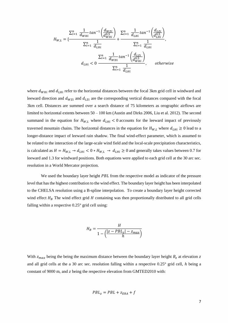
where 𝑑𝑊𝐻𝑖 and 𝑑𝐿𝐻𝑖 refer to the horizontal distances between the focal 3km grid cell in windward and

leeward direction and 𝑑𝑊𝑍𝑖 and 𝑑𝐿𝑍𝑖 are the corresponding vertical distances compared with the focal

3km cell. Distances are summed over a search distance of 75 kilometers as orographic airflows are

limited to horizontal extents between 50 – 100 km (Austin and Dirks 2006, Liu et al. 2012). The second

summand in the equation for 𝐻𝑊,𝐿 where 𝑑𝐿𝐻𝑖 < 0 accounts for the leeward impact of previously

traversed mountain chains. The horizontal distances in the equation for 𝐻𝑊,𝐿 where 𝑑𝐿𝐻𝑖 ≥ 0 lead to a

longer-distance impact of leeward rain shadow. The final wind-effect parameter, which is assumed to

be related to the interaction of the large-scale wind field and the local-scale precipitation characteristics,

is calculated as 𝐻 = 𝐻𝑊,𝐿 → 𝑑𝐿𝐻𝑖 < 0 ∗ 𝐻𝑊,𝐿 → 𝑑𝐿𝐻𝑖 ≥ 0 and generally takes values between 0.7 for

leeward and 1.3 for windward positions. Both equations were applied to each grid cell at the 30 arc sec.

resolution in a World Mercator projection.

We used the boundary layer height 𝑃𝐵𝐿 from the respective model as indicator of the pressure

level that has the highest contribution to the wind effect. The boundary layer height has been interpolated

to the CHELSA resolution using a B-spline interpolation. To create a boundary layer height corrected

wind effect 𝐻𝐵 The wind effect grid 𝐻 containing was then proportionally distributed to all grid cells

falling within a respective 0.25° grid cell using:

𝐻𝐵 =𝐻

1 − (|𝑧 − 𝑃𝐵𝐿𝑧| − 𝑧𝑚𝑎𝑥

ℎ)

With 𝑧𝑚𝑎𝑥 being the being the maximum distance between the boundary layer height 𝐵𝑧 at elevation 𝑧

and all grid cells at the a 30 arc sec. resolution falling within a respective 0.25° grid cell, ℎ being a

constant of 9000 m, and 𝑧 being the respective elevation from GMTED2010 with:

𝑃𝐵𝐿𝑧 = 𝑃𝐵𝐿 + 𝑧𝐸𝑅𝐴 + 𝑓

8

𝐵 being the height of the daily means of the boundary layer from the respective model, 𝑧𝐸𝑅𝐴 being the

elevation of the model grid cell. The boundary layer height provided by ECMWF, which is used in the

observational dataset is based on the Richardson number (Vogelezang and Holtslag 1996) which is

usually at the lower end of the elevational spectrum compared to other methods (von Engeln and

Teixeira 2013). We therefore tuned our model by adding a constant of 500 m similar to the approach in

the original CHELSA algorithm (Karger et al. 2017).

Although the wind effect algorithm can distinguish between the windward and leeward sites of

an orographic barrier, it cannot distinguish extremely isolated valleys in high mountain areas (Frei and

Schär 1998). Such dry valleys are situated in areas where the wet air masses flow over an orographic

barrier and are prevented from flowing into deep valleys (Frei and Schär 1998). These effects are

however mainly confined to large mountain ranges, and are not as prominent in intermediate mountain

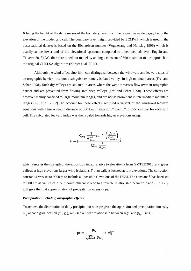
ranges (Liu et al. 2012). To account for these effects, we used a variant of the windward leeward

equations with a linear search distance of 300 km in steps of 5° from 0° to 355° circular for each grid

cell. The calculated leeward index was then scaled towards higher elevations using:

𝐸 = (

∑ 𝑛𝑖=1

1

𝑑 𝑊𝐻𝑖0.5 𝑡𝑎𝑛−1 (

𝑑𝐿𝑍𝑖

𝑑𝑊𝐻𝑖0.5

)

∑ 𝑛𝑖=1

1𝑑𝐿𝐻𝑖

)

𝑧ℎ

which rescales the strength of the exposition index relative to elevation 𝑧 from GMTED2010, and gives

valleys at high elevations larger wind isolations 𝐸 than valleys located at low elevations. The correction

constant ℎ was set to 9000 m to include all possible elevations of the DEM. The constant ℎ has been set

to 9000 m as values of 𝑧 > ℎ could otherwise lead to a reverse relationship between 𝑧 and 𝐸. 𝐸 ∗ 𝐻𝐵

will give the first approximation of precipitation intensity 𝑝𝐼.

Precipitation including orographic effects

To achieve the distribution of daily precipitation rates pr given the approximated precipitation intensity

𝑝𝐼𝑐 at each grid location (𝑥𝑐 , 𝑦𝑐), we used a linear relationship between 𝑝𝑚𝑐𝑜𝑟 and 𝑝𝐼𝑐 using:

pr = 𝑝𝐼𝑐

1𝑛

∑ 𝑛𝑖=1 𝑝𝐼𝑐𝑖

∗ 𝑝𝑚𝑐𝑜𝑟

9

where 𝑛 equals the number of 30 arc sec. grid cells that fall within a 0.25 grid cell. This equations

archives that the data are to scale, e.g. the precipitation at 0.25° resolution exactly matches the mean

precipitation of all 30°sec cells within the range of a 0.25° cell.

Observational dataset

As observational dataset we used a downscaled version of the ERA5-Land reanalysis for temperatures.

The downscaling uses the same algorithms as described in the methods section. For the precipitation

data we used the daily CHELSA V2 precipitation product (Karger et al., in prep).

Regional climate models

T.B.A.

10

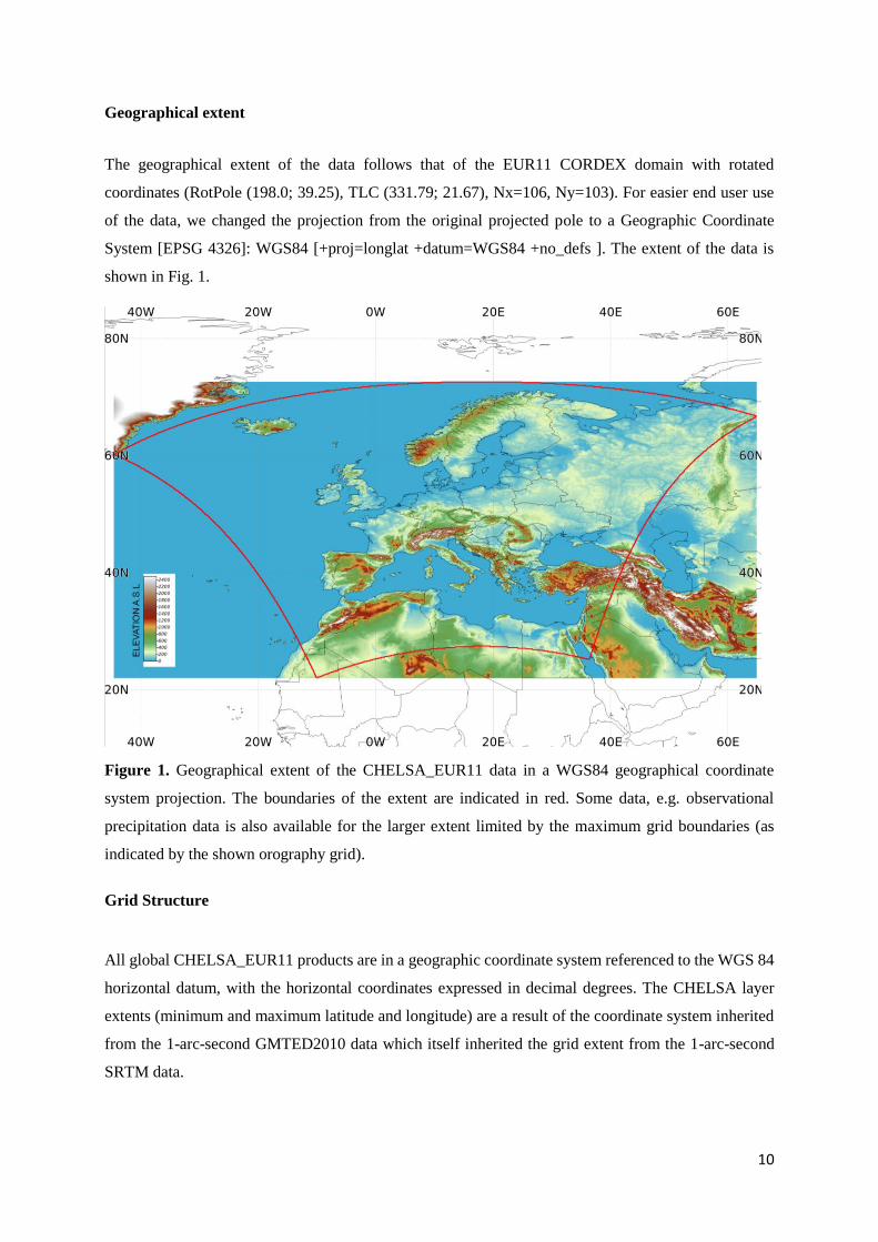
Geographical extent

The geographical extent of the data follows that of the EUR11 CORDEX domain with rotated

coordinates (RotPole (198.0; 39.25), TLC (331.79; 21.67), Nx=106, Ny=103). For easier end user use

of the data, we changed the projection from the original projected pole to a Geographic Coordinate

System [EPSG 4326]: WGS84 [+proj=longlat +datum=WGS84 +no_defs ]. The extent of the data is

shown in Fig. 1.

Figure 1. Geographical extent of the CHELSA_EUR11 data in a WGS84 geographical coordinate

system projection. The boundaries of the extent are indicated in red. Some data, e.g. observational

precipitation data is also available for the larger extent limited by the maximum grid boundaries (as

indicated by the shown orography grid).

Grid Structure

All global CHELSA_EUR11 products are in a geographic coordinate system referenced to the WGS 84

horizontal datum, with the horizontal coordinates expressed in decimal degrees. The CHELSA layer

extents (minimum and maximum latitude and longitude) are a result of the coordinate system inherited

from the 1-arc-second GMTED2010 data which itself inherited the grid extent from the 1-arc-second

SRTM data.

11

Grid extent:

Resolution 0.0083333333

West extent (minimum X-coordinate,

longitude):

-44.6376394303

South extent (minimum Y-coordinate,

latitude)

21.9623606633

East extent (maximum X-coordinate,

longitude)

64.9206934648

North extent (maximum Y-coordinate,

latitude)

72.6040271274

Rows 6078

Columns 13148

Note that because of the pixel center referencing of the input GMTED2010 data the full extent of each

CHELSA grid as defined by the outside edges of the pixels differs from an integer value of latitude or

longitude by 0.000138888888 degree (or 1/2 arc-second). Users of products based on the legacy

GTOPO30 product should note that the coordinate referencing of CHELSA (and GMTED2010) and

GTOPO30 are not the same. In GTOPO30, the integer lines of latitude and longitude fall directly on the

edges of a 30-arc-second pixel. Thus, when overlaying CHELSA with products based on GTOPO30 a

slight shift of 1/2 arc-second will be observed between the edges of corresponding 30-arc-second pixels.

Format and File Organization

CHELSA_EUR11 data files are provided in netCDF-4 format. The CF metadata conventions for

identifying dimension information are followed, so that CHELSA_EUR11 can be used by many tools

that are CF-compliant. Due to the size of the CHELSA_EUR11 archive, most files were compressed

using nccopy –d9 with a maximum deflation level, which does not require an additional unpacking

procedure before the data can be used. The data can be read by all common CF – compliant programs.

In R for example, netCDF-4 files can be read using the ‘ncdf4’ package and the ‘raster’ package (e.g.

g1 <- raster(path_2_netCDF-4_file). The metadata can be read using e.g. gdal (e.g. gdalinfo

path_2_netCDF-4_file) or ncdump –h path_2_netCDF-4_file. In R the metadata can be read using

nc_open(path_2_netCDF-4_file).

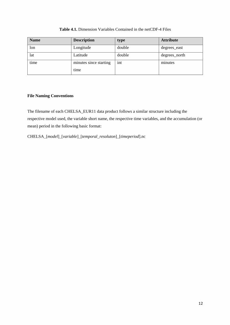
Dimensions

All files contain variables that define the dimensions of longitude, latitude, and time. Dimension

variables have an attribute named “units,” set to an appropriate string defined by the CF

conventions that can be used by applications to identify the dimension.

12

Table 4.1. Dimension Variables Contained in the netCDF-4 Files

Name Description type Attribute

lon Longitude double degrees_east

lat Latitude double degrees_north

time minutes since starting

time

int minutes

File Naming Conventions

The filename of each CHELSA_EUR11 data product follows a similar structure including the

respective model used, the variable short name, the respective time variables, and the accumulation (or

mean) period in the following basic format:

CHELSA_[model]_[variable]_[temporal_resoluton]_[timeperiod].nc

13

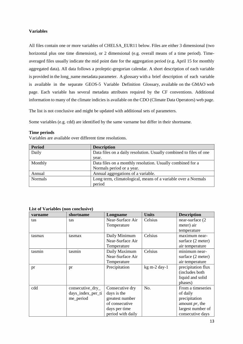
Variables

All files contain one or more variables of CHELSA_EUR11 below. Files are either 3 dimensional (two

horizontal plus one time dimension), or 2 dimensional (e.g. overall means of a time period). Time-

averaged files usually indicate the mid point date for the aggregation period (e.g. April 15 for monthly

aggregated data). All data follows a proleptic-gregorian calendar. A short description of each variable

is provided in the long_name metadata parameter. A glossary with a brief description of each variable

is available in the separate GEOS-5 Variable Definition Glossary, available on the GMAO web

page. Each variable has several metadata attributes required by the CF conventions. Additional

information to many of the climate indicies is available on the CDO (Climate Data Operators) web page.

The list is not conclusive and might be updated with additional sets of parameters.

Some variables (e.g. cdd) are identified by the same varname but differ in their shortname.

Time periods

Variables are available over different time resolutions.

Period Description

Daily Data files on a daily resolution. Usually combined to files of one

year.

Monthly Data files on a monthly resolution. Usually combined for a

Normals period or a year.

Annual Annual aggregations of a variable.

Normals Long term, climatological, means of a variable over a Normals

period

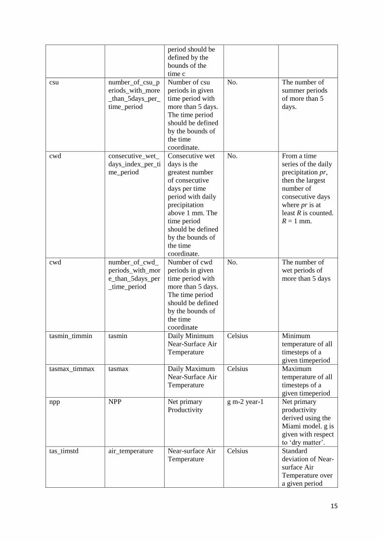
List of Variables (non conclusive)

varname shortname Longname Units Description

tas tas Near-Surface Air

Temperature

Celsius near-surface (2

meter) air

temperature

tasmax tasmax Daily Minimum

Near-Surface Air

Temperature

Celsius maximum near-

surface (2 meter)

air temperature

tasmin tasmin Daily Maximum

Near-Surface Air

Temperature

Celsius minimum near-

surface (2 meter)

air temperature

pr pr Precipitation kg m-2 day-1 precipitation flux

(includes both

liquid and solid

phases)

cdd consecutive_dry_

days_index_per_ti

me_period

Consecutive dry

days is the

greatest number

of consecutive

days per time

period with daily

No. From a timeseries

of daily

precipitation

amount pr, the

largest number of

consecutive days

14

precipitation

amount below

100 mm. The time

period should be

defined by the

bounds of the

time coordinate.

where pr is less

than R is counted.

R is set to = 1 kg

m-2.

cdd number_of_cdd_p

eriods_with_more

_than_5days_per_

time_period

Number of cdd

periods in given

time period with

more than 5 days.

The time period

should be defined

by the bounds of

the time

coordinate.

No. Number of dry

periods of more

than 5 days

cfd consecutive_frost

_days_index_per_

time_period

Consecutive frost

days index is the

greatest number

of consecutive

frost days in a

given time period.

Frost days is the

number of days

where minimum

of temperature is

below 0 degree

Celsius. The time

period should be

defined by the

bounds of the

time coord.

No. From a time

series of the

daily minimum

near-surface air

temperature

tasmin, then the

largest number

of consecutive

days where

tasmin<0°C is

counted

cfd number_of_cfd_p

eriods_with_more

_than_5days_per_

time_period

Number of cfd

periods in given

time period with

more than 5 days.

The time period

should be defined

by the bounds of

the time

coordinate.

No. The number of

frost periods of

more than 5 days

csu consecutive_sum

mer_days_index_

per_time_period

consecutive

summer days

index is the

greatest number

of consecutive

summer days in a

given time period.

Summer days is

the number of

days where

maximum of

temperature is

above 25 degree

Celsius. The time

No. From a time

series of the

daily maximum

temperature

tasmax, the

largest number

of consecutive

days where

tasmax>T is

counted. T =

25°C.

15

period should be

defined by the

bounds of the

time c

csu number_of_csu_p

eriods_with_more

_than_5days_per_

time_period

Number of csu

periods in given

time period with

more than 5 days.

The time period

should be defined

by the bounds of

the time

coordinate.

No. The number of

summer periods

of more than 5

days.

cwd consecutive_wet_

days_index_per_ti

me_period

Consecutive wet

days is the

greatest number

of consecutive

days per time

period with daily

precipitation

above 1 mm. The

time period

should be defined

by the bounds of

the time

coordinate.

No. From a time

series of the daily

precipitation pr,

then the largest

number of

consecutive days

where pr is at

least R is counted.

R = 1 mm.

cwd number_of_cwd_

periods_with_mor

e_than_5days_per

_time_period

Number of cwd

periods in given

time period with

more than 5 days.

The time period

should be defined

by the bounds of

the time

coordinate

No. The number of

wet periods of

more than 5 days

tasmin_timmin tasmin Daily Minimum

Near-Surface Air

Temperature

Celsius Minimum

temperature of all

timesteps of a

given timeperiod

tasmax_timmax tasmax Daily Maximum

Near-Surface Air

Temperature

Celsius Maximum

temperature of all

timesteps of a

given timeperiod

npp NPP Net primary

Productivity

g m-2 year-1 Net primary

productivity

derived using the

Miami model. g is

given with respect

to ‘dry matter’.

tas_timstd air_temperature Near-surface Air

Temperature

Celsius Standard

deviation of Near-

surface Air

Temperature over

a given period

16

tasmax_timstd air_temperature Daily Maximum

Near-Surface Air

Temperature

Celsius Standard

deviation of Daily

Maximum Near-

Surface Air

Temperature over

a given period

tasmin_timstd air_temperature Daily Minimum

Near-Surface Air

Temperature

Celsius Standard

deviation of Daily

Minimum Near-

Surface Air

Temperature over

a given period

pr_timstd pr Precipitation kg m-2 day-1 Standard

deviation of

Precipitation over

a given period

References

Austin, G. L. and Dirks, K. N. 2006. Topographic Effects on Precipitation. - In: Encyclopedia of

Hydrological Sciences. American Cancer Society, in press.

Daly, C. et al. 1997. The PRISM approach to mapping precipitation and temperature. - Proc 10th AMS

Conf Appl. Climatol.: 20–23.

Frei, C. and Schär, C. 1998. A precipitation climatology of the Alps from high-resolution rain-gauge

observations. - Int. J. Climatol. 18: 873–900.

Karger, D. N. et al. 2017. Climatologies at high resolution for the earth’s land surface areas. - Sci.

Data 4: 170122.

Liu, M. et al. 2012. Interaction of valleys and circulation patterns (CPs) on small-scale spatial

precipitation distribution in the complex terrain of southern Germany. - Hydrol. Earth Syst.

Sci. Discuss. in press.

Press, W. H. et al. 1989. Numerical recipes. - Cambridge University Press Cambridge.

Vogelezang, D. H. P. and Holtslag, A. A. M. 1996. Evaluation and model impacts of alternative

boundary-layer height formulations. - Bound.-Layer Meteorol. 81: 245–269.

von Engeln, A. and Teixeira, J. 2013. A Planetary Boundary Layer Height Climatology Derived from

ECMWF Reanalysis Data. - J. Clim. 26: 6575–6590.