High-Quality Volumetric Reconstruction on Optimal Lattices ...torsten/Publications/Papers/ev09-1.pdf · High-Quality Volumetric Reconstruction on Optimal Lattices for Computed Tomography

Eurographics/ IEEE-VGTC Symposium on Visualization 2009H.-C. Hege, I. Hotz, and T. Munzner(Guest Editors)

Volume 28 (2009), Number 3

High-Quality Volumetric Reconstruction on Optimal Lattices

for Computed Tomography

Bernhard Finkbeiner1, Usman R. Alim1, Dimitri Van De Ville2, and Torsten Möller1

1Simon Fraser University, Canada2University of Geneva, Switzerland

Abstract

Within the context of emission tomography, we study volumetric reconstruction methods based on the Expectation

Maximization (EM) algorithm. We show, for the first time, the equivalence of the standard implementation of the

EM-based reconstruction with an implementation based on hardware-accelerated volume rendering for nearest-

neighbor (NN) interpolation. This equivalence suggests that higher-order kernels should be used with caution and

do not necessarily lead to better performance. We also show that the EM algorithm can easily be adapted for

different lattices, the body-centered cubic (BCC) one in particular. For validation purposes, we use the 3D version

of the Shepp-Logan synthetic phantom, for which we derive closed-form analytical expressions of the projection

data. The experimental results show the theoretically-predicted optimality of NN interpolation in combination with

the EM algorithm, for both the noiseless and the noisy case. Moreover, reconstruction on the BCC lattice leads to

superior accuracy, more compact data representation, and better noise reduction compared to the Cartesian one.

Finally, we show the usefulness of the proposed method for optical projection tomography of a mouse embryo.

Categories and Subject Descriptors (according to ACM CCS): Image Processing and Computer Vision [I.4.5]: Re-construction Transform methods—

1. Introduction

3D Computed Tomography (CT) provides a way to recon-struct volumetric data from a set of 2D projections of the3D object acquired at various projection angles. The Maxi-mum Likelihood Expectation Maximization (EM) algorithmis a widely used CT method for image reconstruction inemission tomography (ET). The EM algorithm is an iter-ative method that consists of three steps in each iteration:forward projection, correction, and back-projection. The for-ward projection can be conveniently implemented as volumerendering that enables an implementation of the EM algo-rithm on commodity graphics hardware that delivers veryhigh performance at low hardware costs [CM03, Xu07].

Volume rendering usually seeks to reconstruct acontinuous-domain representation from discrete samplesstored on a regular lattice. Reconstruction is achieved byconvolving the discrete samples with a continuous recon-struction kernel. Obviously, the quality of the reconstruc-tion depends on the chosen reconstruction kernel. In general,

higher-order kernels that use a larger neighborhood deliverbetter quality than lower-order ones. This intuitive fact isusually adapted by using trilinear interpolation when imple-menting the forward projection in the EM algorithm within ahardware-accelerated volume rendering framework [CM03].

In Section 3 of this paper, we will show that a volume ren-dering implementation of the EM algorithm is correct if andonly if it uses nearest-neighbour (NN) interpolation. Higher-order reconstruction kernels are not compatible with stan-dard EM. To the best of our knowledge this is a novel result.

We substantiate this result empirically with several testsin Section 5 demonstrating that NN interpolation achievesmost accurate results compared to higher-order filters.

To accelerate the algorithm, we implement the EM algo-rithm using commodity graphics hardware. Since the EMalgorithm is not bound to a specific lattice, we extend theimplementation to the BCC lattice that is known to havebetter sampling properties than the Cartesian (CC) lattice.This enables reconstruction of volumetric data directly on

c© 2009 The Author(s)Journal compilation c© 2009 The Eurographics Association and Blackwell Publishing Ltd.Published by Blackwell Publishing, 9600 Garsington Road, Oxford OX4 2DQ, UK and350 Main Street, Malden, MA 02148, USA.

Finkbeiner et al. / High-Quality Volumetric Reconstruction on Optimal Lattices for Computed Tomography

a BCC lattice without the need to change acquisition de-vices. We therefore pave the way to a more wide-spreadproduction of data sampled on the BCC lattice: By usinga BCC lattice instead of a CC lattice, either a reduction of29% of the samples without any loss of information can beachieved [TMG01], or more detail can be captured for thesame number of samples.

The three major contributions of our work are as follows:

First, we implement the EM algorithm using volumerendering and show in Section 3 that the traditional dis-crete representation of the EM algorithm is replaced by acontinuous-domain one using a volume rendering frame-work. We show that this requires the use of a NN filter.

Second, in Section 5 we show that volumetric data recon-structed on a BCC lattice deliver higher accuracy and betternoise reduction compared to the CC lattice.

Third, our GPU implementation is two orders of magni-tude faster than a reference CPU implementation: large vol-umes with approximately 130 million samples are recon-structed within less than an hour compared to several days.

We test our method using an analytical phantom and areal-world dataset; i.e., we use the 3D version of the wellknown Shepp-Logan (SL) phantom [SL74] and we deriveanalytical expressions for the ideal 2D projection data. Fur-thermore, we employ data from a new modality where pro-jections of a mouse embryo were acquired using optical pro-jection tomography (OPT) [Sha04].

2. Related Work

Algorithms for CT reconstruction can be split into two cat-egories: analytical and iterative methods. Analytical meth-ods invert the Radon transform in a single step and includeback-projection methods such as Filtered Back Projection(FBP) [Dea83,FDK84]. They only work reliably if the noiseis limited; e.g., for transmission tomography. Iterative meth-ods, on the other hand, optimize a criterion to reconstructthe volume; e.g., the Algebraic Reconstruction Technique(ART) [GBH70] or the EM algorithm [SV82] alternate be-tween forward and back-projections. Iterative procedures arecomputationally expensive, but the criterion can be chosen toimprove robustness in the presence of noise [LM03], whichis clearly the case for ET.

There are several CT methods that have been success-fully ported to the GPU improving reconstruction times[CM03, XM07b]. However, all these methods work on thestandard CC lattice and/or suffer from the poor resolutionof 8 bits of the earlier GPU’s framebuffer. An excellentoverview can be found in Sitek’s tutorial [Sit07] and in Xu’sthesis [Xu07]. None of these methods have investigated theinfluence of different filter kernels (and mostly used linearinterpolation). In contrast, we show that highest quality isachieved when using a NN filter.

The use of BCC lattices in tomography research is notnew [ML95, MY96]. Matej et al. [ML95] used spherically-symmetric volume elements (blobs) introducing computa-tional overhead due to the overlap. Mueller et al. [MY96]employed the BCC lattice to reduce the computational coststo a factor of 70.5% of the equivalent CC lattice. More recentwork by Xu et al. [XM07a] uses commodity graphics hard-ware to accelerate the FBP algorithm using BCC lattices.As mentioned above, this method is not reliable when re-constructing from noisy projections. Iterative methods thatcan deal better with noise often require a forward projec-tion step in every iteration. Forward projection, however, in-volves rendering of a volume; i.e., it involves reconstructionfrom the volume on the underlying lattice with a kernel.

Since we use the EM algorithm (which is an iterativemethod) in a rendering framework, the forward projectionis basically achieved via volume rendering. Volume render-ing involves reconstruction of a continuous-domain functionfrom discrete samples lying on a regular lattice. Theußl et

al. [TMG01] were the first to use BCC lattices together witha spherical extension of reconstruction filters in the area ofvolume rendering. However, visual results were not convinc-ing and since then several filters for the BCC lattice havebeen proposed: box splines [EDM04, EVM08], a prefilter-ing operator followed by a Gaussian filter [Csé05] and a B-spline filter [CH06], and BCC-splines [Csé08]. In this paperwe choose box splines since they guarantee approximationorder and are numerically stable. On the CC side we employthe commonly used B-splines.

3. Computed Tomography

We present a brief overview of the EM algorithm, firstin its traditional discrete form as introduced by Shepp et

al. [SV82] and then in a continuous form that can be adaptedfor use in a volume rendering framework.

3.1. EM Reconstruction

The goal of image reconstruction in ET is to estimate acontinuous 3D activity distribution from discrete measure-ments that correspond to some integral transformation ofthe activity distribution. Lewitt et al. [LM03] have classi-fied the models used to represent the data collection processinto three major categories, namely discrete-continuous (D-C), discrete-discrete (D-D) and continuous-continuous (C-C). D-C models are a natural setting for ET and attempt torelate the discrete measurements to the continuous 3D ac-tivity distribution. D-D models are obtained from D-C mod-els by using a finite set of basis functions to represent theunknown activity distribution. A reconstruction algorithm isthen used to estimate the coefficients of the basis functions.C-C models interpret the discrete measurements as samplesof a continuous function in the measurement space and ananalytic formula is used to invert the integral transform inorder to estimate the activity distribution.

c© 2009 The Author(s)Journal compilation c© 2009 The Eurographics Association and Blackwell Publishing Ltd.


Here, we shall focus on the EM algorithm which is basedon a D-D model of data collection; i.e., it treats the acquiredprojections and the reconstruction volume as discrete data.The 3D volume is typically discretized into non-overlappingcubic cells that are tiled such that their centers make up aregular 3D CC lattice. However, the algorithm is not tied toany specific grid and allows the use of non-CC lattices.

We denote by λ (x), the unknown 3D activity distribution.For convenience, we lexicographically order the cells andindex them with j ( j = 1, . . . ,J). Similarly, assuming a totalof I detector bins, we order them lexicographically and indexthem with i (i = 1, . . . , I). We denote the total number of pho-tons detected in bin i as yi and the total activity in cell j as λ j.The stochastic nature of photon detections in a particular binis modeled as a Poisson process that is independent of thephoton arrivals in other bins. In particular, photon arrivalsin bin i follow a Poisson distribution with mean ∑ j ai, jλ j,where the term ai, j models the physics and geometry of theimaging process and represents the probability that a photonemitted anywhere in cell j will be detected in bin i. This al-lows the D-D imaging model to be written as a matrix-vectorproduct given by

E[y] = A · λ , (1)

where y is the column vector (y1, . . . , yI)T consisting of de-

tector counts and λ is the column vector (λ1, . . . , λJ)T con-

sisting of cell activities.

The EM algorithm takes the form of an iterative procedurethat finds the image estimate λ that maximizes the likelihoodof measuring the data y under the imaging model (1). Werefer the reader to [SV82,LC84] for details of the derivation.

If we denote an activity estimate at iteration n as λ(n)

, thenthe equation that updates the activity estimate of cell j, canbe written as

λ(n+1)j =

λ(n)j

∑i ai, j∑

i

ai, jyi

∑k ai,kλ(n)k

. (2)

Let p(n) be the column vector (p(n)1 , . . . , p

(n)I )T that repre-

sents the projection of the activity estimate λ(n)

at iterationn. It is given by

p(n) = A · λ(n)

. (3)

Also, let c(n) be the column vector (y1/ p(n)1 , . . . , yI/ p

(n)I )T

consisting of correction factors. Equation (2) can then be ex-pressed in a more concise form as

λ(n+1)j = λ

(n)j u

(n)j , (4)

where u(n)j =

(AT ·c(n)) j

∑i ai, jand AT is the transpose of A.

The update equations (2) and (4) have a simple interpreta-tion in terms of projection and back-projection operations.In the standard EM framework, the matrix A computes aprojection of the current activity estimate whereas its trans-pose, AT , back-projects correction factors into the volume to

update the estimate. Sometimes, a different back-projectionmatrix BT may be used to accelerate convergence, resultingin a modified reconstruction algorithm that goes by the nameof Dual-Matrix reconstruction. In ET, it accelerates conver-gence by modeling the physics (attenuation, Compton scat-tering, detector blurring) as well as the geometry of the ac-quisition process into the projection matrix A while keepingthe back-projection matrix BT sparse (e.g by modeling ge-ometry only). The projection and back-projection matricesmust form a valid pair as analyzed in [ZG00].

3.2. Volume Rendering Formulation

Volume rendering techniques for tomographic reconstruc-tion have the advantage that they avoid the expensive compu-tation and storage of the systems matrix A, rather, the entriesof the matrix are implicitly computed on the fly during theprojection and back-projection steps. In order to make use ofvolume rendering techniques, we need to write the discretequantities presented in the previous section, in a form that ismore suitable for volume rendering algorithms. In particu-lar, the activity distribution λ (x) and the forward projectionmodel (1) need to be transposed into the continuous domain.Towards this end, we formulate the equations in terms ofarbitrary basis functions and highlight the conditions underwhich the continuous-domain representation is equivalent tothe discrete EM framework.

We start by examining the D-C data collection modelwhich treats both the emission density and the detectionprobability as continuously defined functions. Let hi(x) de-note the continuous-domain probability density function thatrepresents the probability that an emission within an in-finitessimal volume at x will be detected in bin i. If we rep-resent the continuous-domain emission density as a linearcombination of a finite number of basis functions, the con-tinuous analogue of the discrete imaging model (1) can bewritten as

gi =∫

R3hi(x)

(

∑ jλ jφ j(x)

)

dx, (5)

where gi denotes the total number of photons detected inbin i under a continuous imaging model, φ j(x) is the basisfunction corresponding to cell j and λ j is the correspondingcoefficient. Here, we have not placed any restrictions on thechoice of basis functions. Any set of functions that form avalid basis can be used.

An entry of the matrix A represents the average proba-bility that an emission from cell j will be detected in bini [LM03]. It can be obtained through hi(x) by integratingover the volume occupied by cell j; i.e.,

ai, j =∫

R3hi(x)χ j(x)dx, (6)

where χ j(x) denotes the characteristic function of cell j. Itis unity within the volume of the cell and zero elsewhere.

Using (6) and the D-D projection model of the EM frame-work (1), we can write the expected total number of photons



detected in bin i as

∑ jλ jai, j = ∑ j

λ j

(

∫

R3hi(x)χ j(x)dx

)

=∫

R3hi(x)

(

∑ jλ jχ j(x)

)

dx.

(7)

By comparing this with the continuous imagingmodel (5), we observe that if we use the characteristicfunctions χ j(x) as basis functions along with the total cell

emissions λ j as the corresponding coefficients, the con-tinuous imaging model becomes equivalent to the discreteformulation of the EM framework. Thus, a continuousimaging model that makes use of NN interpolation for theemission density and treats the integration kernel hi(x) asa continuously defined function, can safely be used as aprojector in an EM reconstruction framework. Higher-orderinterpolation schemes are incompatible. This should comeas no surprise since the EM formulation capitalizes on theadditive property of independent Poisson distributions. Anatural way to achieve this independence is to assume anunderlying piecewise-constant emission density.

The back-projection step can also be expressed in an in-tegral form similar to (7). Taking (6) and substituting itinto (2), we see that the total unnormalized correction fac-tor back-projected to cell j is given by

∑i

ciai, j = ∑i

(

∫

R3cihi(x)χ j(x)dx

)

. (8)

Equations (7) and (8) are in a more suitable form sincevolume rendering algorithms are fine tuned for the purposeof computing such integrals.

In ET modalities, a collimator is usually employed thatonly allows photons traveling perpendicular to the detectorplane to pass through. If we further neglect the effects ofphoton scattering, the integration kernel hi(x) is non-zerowithin a cuboid-shaped beam perpendicular to the detectorplane and zero outside. Forward projection (7) can thereforebe efficiently computed via volume rendering using ortho-graphic projection and an emission-only integrator that sam-ples the volume along rays perpendicular to the image plane.Similarly, the back-projection (8) can be evaluated by treat-ing each image plane of correction factors as a light sourceand tracing rays through the volume, accumulating their con-tribution at each cell. In such a volume rendering based ap-proach for computing the forward and back-projection, ifthe integrands are sampled at the same locations, we have amatched projector/back-projector pair as in (4). On the otherhand, in hardware-accelerated reconstruction, the usual ap-proach is to use a smaller step size for the forward projectionand an approximate evaluation of the back-projection step,thus leading to an unmatched approach.

As mentioned earlier, this formulation can be generalizedto any 3D lattice. Once the lattice is determined, the onlyadjustment needed is in the choice of the characteristic func-tion χ j(x), which changes according to the lattice’s Voronoi

cell. In our case we choose the CC and BCC lattices whichhave the cube and the truncated octahedron as their Voronoicells respectively. Therefore, χ j(x) is the NN interpolationkernel of the lattice.

4. Hardware-Based Implementation

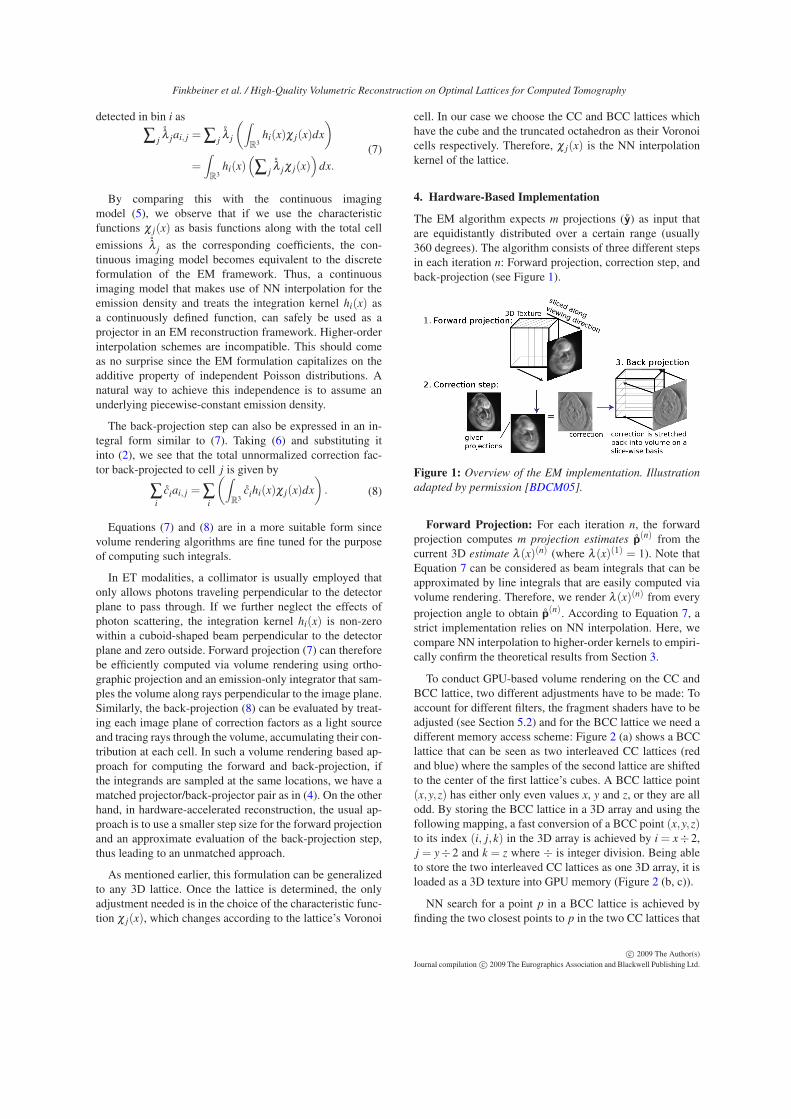
The EM algorithm expects m projections (y) as input thatare equidistantly distributed over a certain range (usually360 degrees). The algorithm consists of three different stepsin each iteration n: Forward projection, correction step, andback-projection (see Figure 1).

Figure 1: Overview of the EM implementation. Illustration

adapted by permission [BDCM05].

Forward Projection: For each iteration n, the forwardprojection computes m projection estimates p(n) from thecurrent 3D estimate λ (x)(n) (where λ (x)(1) = 1). Note thatEquation 7 can be considered as beam integrals that can beapproximated by line integrals that are easily computed viavolume rendering. Therefore, we render λ (x)(n) from everyprojection angle to obtain p(n). According to Equation 7, astrict implementation relies on NN interpolation. Here, wecompare NN interpolation to higher-order kernels to empiri-cally confirm the theoretical results from Section 3.

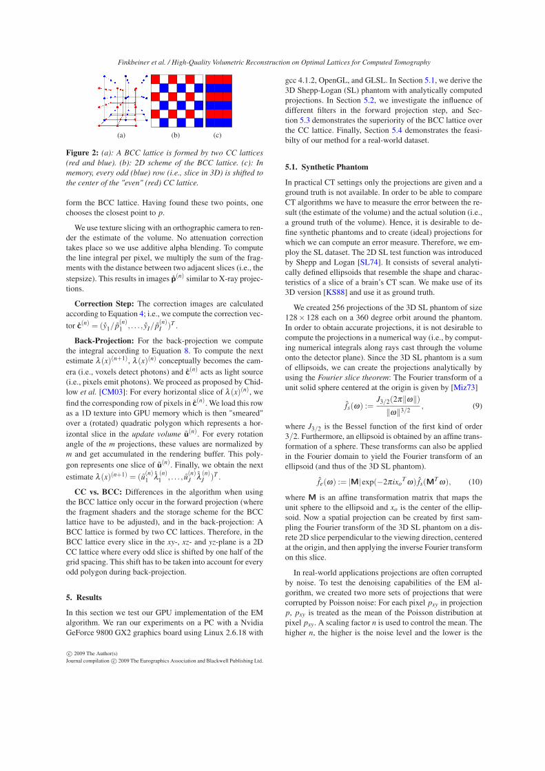
To conduct GPU-based volume rendering on the CC andBCC lattice, two different adjustments have to be made: Toaccount for different filters, the fragment shaders have to beadjusted (see Section 5.2) and for the BCC lattice we need adifferent memory access scheme: Figure 2 (a) shows a BCClattice that can be seen as two interleaved CC lattices (redand blue) where the samples of the second lattice are shiftedto the center of the first lattice’s cubes. A BCC lattice point(x,y,z) has either only even values x, y and z, or they are allodd. By storing the BCC lattice in a 3D array and using thefollowing mapping, a fast conversion of a BCC point (x,y,z)to its index (i, j,k) in the 3D array is achieved by i = x÷2,j = y÷ 2 and k = z where ÷ is integer division. Being ableto store the two interleaved CC lattices as one 3D array, it isloaded as a 3D texture into GPU memory (Figure 2 (b, c)).

NN search for a point p in a BCC lattice is achieved byfinding the two closest points to p in the two CC lattices that



(a) (b) (c)

Figure 2: (a): A BCC lattice is formed by two CC lattices

(red and blue). (b): 2D scheme of the BCC lattice. (c): In

memory, every odd (blue) row (i.e., slice in 3D) is shifted to

the center of the "even" (red) CC lattice.

form the BCC lattice. Having found these two points, onechooses the closest point to p.

We use texture slicing with an orthographic camera to ren-der the estimate of the volume. No attenuation correctiontakes place so we use additive alpha blending. To computethe line integral per pixel, we multiply the sum of the frag-ments with the distance between two adjacent slices (i.e., thestepsize). This results in images p(n) similar to X-ray projec-tions.

Correction Step: The correction images are calculatedaccording to Equation 4; i.e., we compute the correction vec-

tor c(n) = (y1/ p(n)1 , . . . , yI/ p

(n)I )T .

Back-Projection: For the back-projection we computethe integral according to Equation 8. To compute the nextestimate λ (x)(n+1), λ (x)(n) conceptually becomes the cam-era (i.e., voxels detect photons) and c(n) acts as light source(i.e., pixels emit photons). We proceed as proposed by Chid-low et al. [CM03]: For every horizontal slice of λ (x)(n), wefind the corresponding row of pixels in c(n). We load this rowas a 1D texture into GPU memory which is then "smeared"over a (rotated) quadratic polygon which represents a hor-izontal slice in the update volume u(n). For every rotationangle of the m projections, these values are normalized bym and get accumulated in the rendering buffer. This poly-gon represents one slice of u(n). Finally, we obtain the next

estimate λ (x)(n+1) = (u(n)1 λ

(n)1 , . . . , u

(n)J λ

(n)J )T .

CC vs. BCC: Differences in the algorithm when usingthe BCC lattice only occur in the forward projection (wherethe fragment shaders and the storage scheme for the BCClattice have to be adjusted), and in the back-projection: ABCC lattice is formed by two CC lattices. Therefore, in theBCC lattice every slice in the xy-, xz- and yz-plane is a 2DCC lattice where every odd slice is shifted by one half of thegrid spacing. This shift has to be taken into account for everyodd polygon during back-projection.

5. Results

In this section we test our GPU implementation of the EMalgorithm. We ran our experiments on a PC with a NvidiaGeForce 9800 GX2 graphics board using Linux 2.6.18 with

gcc 4.1.2, OpenGL, and GLSL. In Section 5.1, we derive the3D Shepp-Logan (SL) phantom with analytically computedprojections. In Section 5.2, we investigate the influence ofdifferent filters in the forward projection step, and Sec-tion 5.3 demonstrates the superiority of the BCC lattice overthe CC lattice. Finally, Section 5.4 demonstrates the feasi-bilty of our method for a real-world dataset.

5.1. Synthetic Phantom

In practical CT settings only the projections are given and aground truth is not available. In order to be able to compareCT algorithms we have to measure the error between the re-sult (the estimate of the volume) and the actual solution (i.e.,a ground truth of the volume). Hence, it is desirable to de-fine synthetic phantoms and to create (ideal) projections forwhich we can compute an error measure. Therefore, we em-ploy the SL dataset. The 2D SL test function was introducedby Shepp and Logan [SL74]. It consists of several analyti-cally defined ellipsoids that resemble the shape and charac-teristics of a slice of a brain’s CT scan. We make use of its3D version [KS88] and use it as ground truth.

We created 256 projections of the 3D SL phantom of size128× 128 each on a 360 degree orbit around the phantom.In order to obtain accurate projections, it is not desirable tocompute the projections in a numerical way (i.e., by comput-ing numerical integrals along rays cast through the volumeonto the detector plane). Since the 3D SL phantom is a sumof ellipsoids, we can create the projections analytically byusing the Fourier slice theorem: The Fourier transform of aunit solid sphere centered at the origin is given by [Miz73]

fs(ω) :=J3/2(2π‖ω‖)

‖ω‖3/2, (9)

where J3/2 is the Bessel function of the first kind of order3/2. Furthermore, an ellipsoid is obtained by an affine trans-formation of a sphere. These transforms can also be appliedin the Fourier domain to yield the Fourier transform of anellipsoid (and thus of the 3D SL phantom).

fe(ω) := |M|exp(−2πixoT ω) fs(M

T ω), (10)

where M is an affine transformation matrix that maps theunit sphere to the ellipsoid and xo is the center of the ellip-soid. Now a spatial projection can be created by first sam-pling the Fourier transform of the 3D SL phantom on a dis-rete 2D slice perpendicular to the viewing direction, centeredat the origin, and then applying the inverse Fourier transformon this slice.

In real-world applications projections are often corruptedby noise. To test the denoising capabilities of the EM al-gorithm, we created two more sets of projections that werecorrupted by Poisson noise: For each pixel pxy in projectionp, pxy is treated as the mean of the Poisson distribution atpixel pxy. A scaling factor n is used to control the mean. Thehigher n, the higher is the noise level and the lower is the



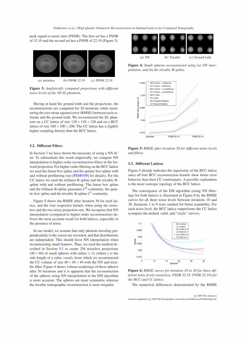
peak signal-to-noise ratio (PSNR). The first set has a PSNRof 32.19 and the second set has a PSNR of 22.19 (Figure 3).

(a) noiseless (b) PSNR 32.19 (c) PSNR 22.19

Figure 3: Analytically computed projections with different

noise levels of the 3D SL phantom.

Having at hand the ground truth and the projections, thereconstructions are computed for 30 iterations while moni-toring the root mean squared error (RMSE) between each es-timate and the ground truth. We reconstructed the SL phan-tom on a CC lattice of size 128× 128× 128 and on a BCClattice of size 100×100×200. The CC lattice has a slightlyhigher sampling density than the BCC lattice.

5.2. Different Filters

In Section 3 we have shown the necessity of using a NN fil-ter. To substantiate this result empirically, we compare NNinterpolation to higher-order reconstruction filters in the for-ward projection. For higher-order filtering on the BCC latticewe used the linear box spline and the quintic box spline withand without prefiltering (see [FEMV09] for details). For theCC lattice we used the trilinear B-spline and the tricubic B-spline with and without prefiltering. The linear box splineand the trilinear B-spline guarantee C0 continuity, the quin-tic box spline and the tricubic B-spline C2 continuity.

Figure 5 shows the RMSE after iteration 30 for each lat-tice, and the four respective kernels when using the noise-less and the two noisy projection sets. We recognize that NNinterpolation (compared to higher-order reconstruction) de-livers the most accurate result for both lattices, especially inthe presence of noise.

In our model, we assume that only photons traveling per-pendicularly to the sensor are recorded, and that distributionsare independent. This should favor NN interpolation whenreconstructing small features. Thus, we used the method de-scribed in Section 5.1 to create 256 noiseless projections(40× 40) of small spheres with radius ≈ 2x (where x is theside length of a cubic voxel), from which we reconstructedthe CC volume of size 40× 40× 40 with the NN and tricu-bic filter. Figure 4 shows volume renderings of these spheresafter 30 iterations and it is apparent that the reconstructionof the spheres using NN interpolation in the EM algorithmis more accurate. The spheres are more symmetric whereasthe tricubic tomographic reconstruction is more irregular.

(a) NN (b) Tricubic (c) Ground truth

Figure 4: Small spheres reconstructed using (a) NN inter-

polation, and (b) the tricubic B-spline.

noiseless PSNR 32.19 PSNR 22.19

0.075

0.08

0.085

0.09

0.095

RM

SE

aft

er

ite

ratio

n 3

0

BCC Quintic − prefiltering

CC Tricubic − prefiltering

BCC Quintic − no prefiltering

CC Tricubic − no prefiltering

BCC Linear

CC Linear

BCC Nearest Neighbor

CC Nearest Neighbor

Figure 5: RMSE after iteration 30 for different noise levels

and filters.

5.3. Different Lattices

Figure 5 already indicates the superiority of the BCC latticesince all four BCC reconstruction kernels show better errorbehavior than their CC counterparts. A possible explanationis the more isotropic topology of the BCC lattice.

The convergence of the EM algorithm (using NN filter-ing) for both lattices is illustrated in Figure 6 by the RMSEcurves for all three noise levels between iterations 10 and30. Iterations 1 to 9 were omitted for better readability. Foreach noise level, the BCC lattice outperforms the CC lattice(compare the dashed, solid, and “circle” curves).

5 10 15 20 25 30

0.075

0.08

0.085

0.09

0.095

0.1

Iterations

RM

SE

BCC noiseless

CC noiseless

BCC PSNR 32.19

CC PSNR 32.19

BCC PSNR 22.19

CC PSNR 22.19

Figure 6: RMSE curves for iteration 10 to 30 for three dif-

ferent noise levels (noiseless, PSNR 32.19, PSNR 22.19) for

the BCC and CC lattice.

The numerical differences demonstrated by the RMSE



curves are supported by visual results. In the following, weused the projections with a PSNR of 32.19 but similar resultswere obtained for noiseless projections and noisy projectionswith a PSNR of 22.19 and are presented in total in the filesl_results.pdf of the supplementary material.

Figure 8 shows two slices from the reconstructed vol-umes: (a) shows a 128 × 128 slice from the reconstructedCC volume after 30 iterations and (b) and (c) show the corre-sponding slice (100×100) from the reconstructed BCC vol-ume. Note that although the BCC slice has only 100× 100pixels, the physical size of the slice is the same as the size ofthe CC slice. The reason for this is the different topology ofthe BCC lattice. To avoid confusion we therefore show theBCC slice with the same pixel size (b) and the same phys-ical size (c) as the CC slice. In other words, (c) is just anupscaled version of (b). (d-f) show the corresponding slicesof the ground truths (CC and BCC). When comparing the es-timate of the CC volume (a) to the estimate of the BCC vol-ume (b, c) the visual difference is noticable: The BCC slice(b, c) shows less noise than its CC counterpart in (a). Thelast row (g, h) shows the intensity values indicated by thered lines in the middle row. The dashed black lines indicatethe ground truth. Again, (h) shows less noise than (g) anddemonstrates the better noise suppression of the BCC lattice.As a quantitive measure of noise suppression we computedthe variance in the homogeneous dark grey region of the SLphantom. The lower the variance the better the noise sup-pression: For the BCC lattice the variance in the dark greyregion is 0.000277 and for the CC lattice 0.000413, whichshows that the noise suppression for the BCC lattice is al-most twice as good as for the CC lattice.

The presented experiments were also performed with aBCC lattice of size 91×91×182 which is 30% smaller thanthe CC lattice. A BCC lattice of this size can store the sameinformation as the 1283 CC lattice and the results in the sup-plementary file sl_results.pdf show that even this BCC lat-tice performs better than the CC lattice.

5.4. Real-World Data Experiments

We demonstrate the feasibility of tomographic reconstruc-tion on BCC lattices using the GPU by reconstructing a vol-ume from real-world data. We use projections of a mouseembryo that were acquired at the Max-Planck-Institute forMolecular Genetics using OPT. OPT is a method usedto capture objects of the size of 1 to 10 mm diame-ter [SAP∗02] at high spatial resolution and is employedfor three-dimensional imaging of small biological specimenwith optical light. Thus, different wavelengths (i.e., color)can be captured. Applications of OPT are mainly in the fieldof molecular biology and include gene-expression analysis,screening of abnormal anatomy or histology, or pinpointingcells within a tissue [Sha04].

We used 400 scalar OPT scans of a mouse embryo whereeach projection has a resolution of 471 × 696 pixels. Our

GPU implementation is able to reconstruct a high-resolutionvolume (321×474×642 BCC samples, see Figure 7) withinless than one hour (30 iterations). Our reference CPU imple-mentation requires seven days employing eight cores.

Figure 7: Volume rendering of the mouse embryo which was

acquired from 400 OPT scans on a BCC lattice (321×474×642). Red areas indicate the most dense tissue.

(a) CC (b) BCC (c) BCC

(d) CC truth (e) BCC truth (f) BCC truth

0 0.1 0.2 0.3 0.4 0.5 0.6 0.7 0.8 0.9 10

0.2

0.4

0.6

0.8

1

(g) CC profile0 0.1 0.2 0.3 0.4 0.5 0.6 0.7 0.8 0.9 1

0

0.2

0.4

0.6

0.8

1

(h) BCC profile

Figure 8: (a): CC slice of the reconstructed volume. (b):

corresponding BCC slice. (c): upscaled verion of (b). Sec-

ond row: corresponding ground truths. Last row: intensity

profiles indicated by the red lines in (d-f).

6. Conclusion and Future Work

We have established in a mathematical and empirical waythe connection between the standard EM algorithm and the



continuous-domain volume rendering framework using NNinterpolation. This contradicts the intuition that higher-orderfilters lead to higher accuracy; i.e., for the EM algorithm towork best with volume rendering techniques, one has to useNN interpolation. Higher-order reconstruction filters are in-compatible. Note that NN interpolation is also the fastest re-construction scheme due to its small and compact support.

Furthermore, we have demonstrated that volumetric re-construction on the BCC lattice is more accurate and bet-ter suited for noise suppression than traditional reconstruc-tion on CC lattices. The advantage of our method is that theacquired projections are still on 2D Cartesian lattices andtherefore acquisition devices do not need to be changed. Thisresult opens the possibility to a more wide-spread use of op-timal sampling lattices in the areas of computed tomographyand volume rendering.

So far, we have not modeled effects such as scatter correc-tion, collimator blur, and attenuation correction. However,we assume that NN interpolation will also improve resultsbecause of its fundamental connection to the EM algorithm.The investigation of these effects are subject to future work.

Furthermore, we plan to investigate the possibilities of ex-tending the EM algorithm for higher-order filters by match-ing the forward and back-projection for arbitrary reconstruc-tion kernels. This could enable us to use the advantages ofhigher-order filters for CT.

References

[BDCM05] BERGNER S., DAGENAIS E., CELLER A., MÖLLER

T.: Using the physically-based rendering toolkit for medical re-construction. Proceedings of 2005 IEEE Nuclear Science Sym-

posium and Medical Imaging Conference (October 2005), 3022–3026.

[CH06] CSÉBFALVI B., HADWIGER M.: Prefiltered B-splinereconstruction for hardware-accelerated rendering of optimallysampled volumetric data. Vision, Modeling and Visualization

(2006), 325–332.

[CM03] CHIDLOW K., MÖLLER T.: Rapid emission tomogra-phy reconstruction. Workshop on Volume Graphics (VG03) (July2003), 15–26.

[Csé05] CSÉBFALVI B.: Prefiltered Gaussian reconstruction forhigh-quality rendering of volumetric data sampled on a body-centered cubic grid. IEEE Visualization (2005), 40–48.

[Csé08] CSÉBFALVI B.: BCC-splines: Generalization of B-splines for the body-centered cubic lattice. Winter School of

Computer Graphics (2008).

[Dea83] DEANS S. R.: The radon transform and some of its ap-plications. A Wiley-Interscience Publication, New York (1983).

[EDM04] ENTEZARI A., DYER R., MÖLLER T.: Linear and cu-bic box splines for the body centered cubic lattice. Proceedings

of IEEE Visualization (2004), 11–18.

[EVM08] ENTEZARI A., VILLE D. V. D., MÖLLER T.: Practicalbox splines for reconstruction on the body centered cubic lattice.IEEE Transactions on Visualization and Computer Graphics 14,2 (2008), 313–328.

[FDK84] FELDKAMP L. A., DAVIS L., KRESS J. W.: Practicalcone beam algorithm. J. Optical Society of America 1, 6 (6 1984),612–619.

[FEMV09] FINKBEINER B., ENTEZARI A., MÖLLER T., VILLE

D. V. D.: Efficient Volume Rendering on the Body Centered Cu-

bic Lattice Using Box Splines. Tech. Rep. TR 2009-04, SimonFraser University, 3 2009.

[GBH70] GORDON R., BENDER R., HERMAN G. T.: Algebraicreconstruction techniques (ART) for three-dimensional electronmicroscopy and X-ray photography. Journal of Theoretical Biol-

ogy 29, 3 (1970), 471–81.

[KS88] KAK A. C., SLANEY M.: Principles of Computerized

Tomographic Imaging. IEEE Press, 1988.

[LC84] LANGE K., CARSON R.: EM reconstruction algorithmsfor emission and transmission tomography. Journal of Computer

Assisted Tomography 8, 2 (1984), 306–16.

[LM03] LEWITT R. M., MATEJ S.: Overview of methods forimage reconstruction from projections in emission computed to-mography. Proceedings of the IEEE 91, 10 (2003), 1588–1611.

[Miz73] MIZOHATA S.: The Theory of Partial Differential Equa-

tions. Cambridge University Press, 1973.

[ML95] MATEJ S., LEWITT R. M.: Efficient 3D grids forimage reconstruction using spherically-symmetric volume ele-ments. IEEE Transactions on Nuclear Science 42, 4 (1995),1361–1370.

[MY96] MUELLER K., YAGEL R.: The use of dodecahedral gridsto improve the efficiency of the algebraic reconstruction tech-nique (ART). Annals Biomedical Engineering, Special issue,

1996 Annual Conference of the Biomedical Engineering Society

(1996), S–66.

[SAP∗02] SHARPE J., AHLGREN U., PERRY P., HILL B., ROSS

A., HECKSHER-SØRENSEN J., BALDOCK R., DAVIDSON D.:Optical projection tomography as a tool for 3D microscopy andgene expression studies. Science 296 (2002), 541–545.

[Sha04] SHARPE J.: Optical projection tomography. Annual Re-

view of Biomedical Engineering 6 (August 2004), 209–228.

[Sit07] SITEK A.: Programming and medical applications us-ing graphics hardware. Nuclear Science Symposium and Med-

ical Imaging Conference (2007).

[SL74] SHEPP L. A., LOGAN B. F.: Reconstructing interior headtissue from X-ray transmissions. IEEE Transactions on Nuclear

Science 21, 1 (1974), 228–236.

[SV82] SHEPP L. A., VARDI Y.: Maximum likelihood recon-struction for emission tomography. IEEE Transanctions Medical

Imaging 1, 2 (1982), 113–122.

[TMG01] THEUSSL T., MÖLLER T., GRÖLLER E.: Optimal reg-ular volume sampling. Proceedings of IEEE Visualization (2001),91–98.

[XM07a] XU F., MUELLER K.: Applications of optimal sam-pling lattices for volume acquisition via 3D computed tomogra-phy. Volume Graphics Symposium (2007), 57–63.

[XM07b] XU F., MUELLER K.: Real-time 3D computed to-mographic reconstruction using commodity graphics hardware.Physics in Medicine & Biology 52 (2007), 3405–3419.

[Xu07] XU F.: Accelerating Computed Tomography on Graphics

Hardware. PhD thesis, Stony Brook University, Stony Brook,New York, 2007.

[ZG00] ZENG G. L., GULLBERG G. T.: Unmatched projec-tor/backprojector pairs in an iterative reconstruction algorithm.IEEE Transactions on Medical Imaging 19, 5 (2000), 548–555.


Documents

High-Quality Volumetric Reconstruction on Optimal Lattices ...torsten/Publications/Papers/ev09-1.pdf · High-Quality Volumetric Reconstruction on Optimal Lattices for Computed Tomography