Embed Size (px)
Citation preview

Celest Mech Dyn Astr (2013) 116:141–174DOI 10.1007/s10569-013-9479-6
ORIGINAL ARTICLE
High precision symplectic integrators for the SolarSystem
Ariadna Farrés · Jacques Laskar · Sergio Blanes ·Fernando Casas · Joseba Makazaga · Ander Murua
Received: 6 August 2012 / Revised: 12 February 2013 / Accepted: 27 February 2013 /Published online: 3 April 2013© Springer Science+Business Media Dordrecht 2013
Abstract Using a Newtonian model of the Solar System with all 8 planets, we performextensive tests on various symplectic integrators of high orders, searching for the best splittingscheme for long term studies in the Solar System. These comparisons are made in Jacobiand heliocentric coordinates and the implementation of the algorithms is fully detailed forpractical use. We conclude that high order integrators should be privileged, with a preferencefor the new (10, 6, 4) method of Blanes et al. (2013).
Keywords Symplectic integrators · Hamiltonian systems · Planetary motion · Jacobicoordinates · Heliocentric coordinates · Splitting sympletic methods
A. Farrés · J. Laskar (B)Astronomie et Systèmes Dynamiques, IMCCE-CNRS UMR8028,Observatoire de Paris, UPMC, 77 Av. Denfert-Rochereau, 75014 Paris, Francee-mail: [email protected]
A. Farrése-mail: [email protected]
S. BlanesInstituto de Matemática Multidisciplinar, Universitat Politècnica de València,46022 Valencia, Spaine-mail: [email protected]
F. CasasDepartament de Matemàtiques, Institut de Matemàtiques i Aplicacions de Castelló,Universitat Jaume I, 12071 Castellón, Spaine-mail: [email protected]
J. Makazaga · A. MuruaKonputazio Zientziak eta A.A. saila, Informatika Fakultatea, UPV/EHU,Donostia/San Sebastián, Spaine-mail: [email protected]
A. Muruae-mail: [email protected]
123
142 A. Farrés et al.
1 Introduction
Due to their simplicity and stability properties, symplectic integrators have been widelyused for long-term integrations of the Solar System, starting with the work of Wisdom andHolman (1991). In many studies on the formation and evolution of the Solar System, wherelarge numbers of particles are considered, the speed of the integrator is a major constraint andlow order schemes have been often used as in the original scheme of Wisdom and Holman(1991) or Kinoshita et al. (1991) (for a review see Morbidelli 2002).
On the opposite, in the present work we are focusing on high precision symplectic inte-grators that are designed for the computation of long term ephemerides of the Solar System,when one searches to reduce the numerical error of the algorithm to the level of the roundofferror of the machine. These integrators will also be useful for the detailed dynamical studiesof the extra solar planetary system with strong planetary interactions.
The first long term direct numerical integration of a realistic model of the Solar System,including all planets and the effects of general relativity and the Moon was made twentyyears ago over 3 Myr (Quinn et al. 1991) using a high order symmetric multistep method.This solution could be compared with success with the previous averaged solutions of Laskar(1989, 1990a) and confirmed the existence of secular resonances in the Solar System (Laskaret al. 1992). Soon after, using a symplectic integrator with mixed variables (Wisdom andHolman 1991), Sussman and Wisdom (1992) could extend these computation to 100 Myr,confirming the chaotic behaviour of the Solar System discovered with the secular equationsby Laskar (1989, 1990a).
As the Solar System is chaotic, the error in numerical integrations is multiplied by 10 every10 Myr (Laskar 1989). Due to the limited accuracy of the models and initial conditions, it isthus hopeless to obtain a precise solution for the evolution of the Solar System over morethan 100 Myr. The situation is even worse when the full Solar System is considered, asclose encounters among the minor planets induce strong chaotic effects that will limit allpossibilities of computing a precise solution for the planets to about 60 Myr (Laskar et al.2011a,b).
Despite this limitation, there is a strong need for precise ephemerides of the planets fromthe paleoclimate community. Indeed, the variations of the Earth orbital elements inducesome changes in the Earth climate that are reflected in the sedimentary records over millionof years. This mechanism, known as Milankovitch theory (Milankovitch 1941) allows nowto use the astronomical solution for the calibration of the geological time scales throughthe correlation of the variation of orbital and rotational elements of the Earth to geologicalrecords. This method has been successfully used for the Neogene period (Lourens et al.2004) over 23 Myr, and a large effort is pursued at present to extend this study over the fullCenozoic era, up to about 65 Myr. This quest led to search for high order symplectic schemesthat are adapted to these long time computations, where high accuracy is requested (Laskarand Robutel 2001; Laskar et al. 2004, 2011a), but it should be noted that in the latest work,the integration of the Solar System model over 250 Myr,1 including five main asteroids tookmore than 18 months of CPU time. Some improvements of the algorithms were thus needed,and the present paper is the outcome of the studies that we have undertaken in order to searchfor the best integrators for the next generations of numerical solutions. At the same time, wehave compared various sets of coordinates (heliocentric and Jacobi), as the performances ofthese integrators depend on the choice of splitting of the Hamiltonian, and thus of the set of
1 Although it has been demonstrated that a precise solution of the motion of the Earth cannot be computedover more than 60 Myr (Laskar et al. 2011b), the solutions are systematically computed over 250 Myr as somefeatures of the solutions can be trusted over longer times (Laskar et al. 2004, 2011a).
123
High precision symplectic integrators 143
coordinates that correspond to these various splittings. As the integrators that are presentedhere are of high order, they can also be used for refined analysis of the newly discovered extrasolar planetary systems, especially when the planetary interactions in the system are strong.
For the planetary case, when using an appropriate set of coordinates, the equations ofmotion are written as an integrable part HA, that corresponds to the Keplerian motion ofeach planet, and a small perturbation HB , given by the interaction of the planets betweeneach other. Hence, the system falls into the category of Hamiltonian system of the kindH = HA + εHB .
Several splitting integrating schemes that take advantage of this fact to derive efficientintegrators exist in the literature. McLachlan (1995) was the first to present such schemesand was followed independently by Chambers and Murison (2000) and Laskar and Robutel(2001). Most recently (Blanes et al. 2013) derived higher order schemes that present veryinteresting behaviour.
In this paper we describe these different splitting symplectic schemes and compare themfor the case of the Solar System dynamics. We want to see which are the most efficient andaccurate schemes. We will consider the gravitational N-body model and test the differentintegrating schemes against different planetary configurations, to be more specific: the 4inner planets, the 4 outer planets and the 8 planets in the Solar System (Sect. 4).
The Hamiltonian of the gravitational N-body problem H = T (p)+U (q) can be rewrittenas H = HA + εHB , using two different set of canonical coordinates: Jacobi and heliocentriccoordinates (Sect. 3). The main difference between both sets of equations is that in Jacobicoordinates the small perturbation HB depends only on positions while in heliocentric coor-dinates the perturbation depends on both position and velocity. This is why in the literatureJacobi coordinates have been more widely used. In Sect. 5 we describe different symplecticschemes for Jacobi coordinates, and in Sect. 6 other symplectic schemes that are suitablefor heliocentric coordinates. In both sections we describe and compare the different splittingschemes. Finally in Sect. 7 we compare the results for the two different set of coordinates.
2 Splitting symplectic integrators (general overview)
Let H(q, p) be a Hamiltonian system where (q, p) are a set of canonical coordinates (i.e. qare the positions and p the momenta). It is well known that in many mechanical problemsthe Hamiltonian is of the form
H(q, p) = T (p)+ U (q),
which is separable with respect to the local canonical coordinates. Using the Lie formalismwe can write the equations of motion as:
dz
dt= {H, z} = L H z, (1)
where by definition Lχ f := {χ, f } is the differential operator Lχ , z = (q, p) and {·, ·}denotes the Poisson bracket.2
The formal solution of Eq. 1 at time t = τ0 + τ that starts at time t = τ0 is given by
z(τ0 + τ) = exp(τ L H )z(τ0) = exp(τ (LT + LU ))z(τ0). (2)
2 {F,G} = ∑ni=1
∂F∂pi
∂G∂qi
− ∂F∂qi
∂G∂pi
.
123
144 A. Farrés et al.
In general the operators LT and LU do not commute, exp(τ (LT + LU )) �= exp(τ LT )
exp(τ LU ), but we can find coefficients ai , bi such that for a given r ,
exp(τ (LT + LU )) =s∏
i=1
exp(aiτ LT ) exp(biτ LU )+ O(τ r+1). (3)
Using the Baker–Campbell–Hausdorff (BCH) identity we can find relations that the coef-ficients ai , bi must satisfy to have a high order scheme (Koseleff 1993b, 1996). These arethe so-called order conditions. For a given set of coefficients ai , bi satisfying Eq. 3, thecomposition
z(τ ) = S(τ )z(τ0) =s∏
i=1
exp(aiτ LT ) exp(biτ LU )z(τ0), (4)
is a symplectic map of order r .The map S(τ ) is symplectic because it is the product of elementary symplectic maps,
exp(τ LT ) and exp(τ LU ), and has order r because it approximates the exact solution up toorder τ r . We will refer to these kind of symplectic schemes as splitting symplectic integrators.
Some of the main advantages of these kind of integrating schemes are: (a) they are veryeasy to implement; (b) they preserve the symplectic character of the Hamiltonian system;and (c) in general there is no systematic drift on the conservation of the energy during thenumerical integration.
These kind of symplectic schemes have been widely studied throughout the years by sev-eral authors (see Hairer et al. 2006; McLachlan and Quispel 2002 and references therein).As a matter of fact, splitting methods have been designed (often independently) and exten-sively used in fields as diverse as molecular dynamics, simulations of storage rings in particleaccelerators, quantum chemistry and, of course, Celestial Mechanics.
There are several procedures to get the order conditions for the coefficients of the splittingscheme in Eq. 4. These are, generally speaking, large systems of polynomial equations in thecoefficients that are obtained from Eq. 3. Two of the most popular are the recursive applicationof the BCH formula to the composition in Eq. 4, and a generalisation of the theory of rootedtrees used in the analysis of Runge–Kutta methods due to Murua and Sanz-Serna (1999) (seealso Hairer et al. 2006). The latter procedure, while being more systematic than the former, ishowever not appropriate for the case of splitting methods applied to Hamiltonians of the formA + εB. In Blanes et al. (2013) a novel systematic way is proposed based on the so-calledLyndon multi-indices that is well adapted to that case.
Splitting methods of order greater than two involve necessarily some negative coefficientsai and b j (Goldman and Kaper 1996; Sheng 1989; Suzuki 1991). Although this feature doesnot imply in principle any special impediment for the class of systems considered in thispaper, it is clear that the presence of negative coefficients may affect the numerical error andthe maximal step size of the scheme. For this reason, when dealing with high order methods,minimising the size of the negative coefficients and the sum of the absolute value of all thecoefficients will be a critical factor in the choice of one particular set of coefficients.
In this paper we do not intend to give the details on the derivation of the order conditionsor how to find these coefficients. All these issues are analysed in detail in Blanes et al. (2013).Our aim here is to compare the performance of different splitting symplectic schemes for thespecific case of the integration of the Solar System.
If we focus on the motion of the Solar System, or other planetary systems, we have amain massive body in the centre (the Sun) and the other bodies evolve around the centremass following almost Keplerian orbits. We can take advantage of this to build more efficient
123
High precision symplectic integrators 145
schemes. Using an appropriate change of coordinates we can rewrite the Hamiltonian as,H = HK + HI (where |HI | � |HK |), a sum of the Keplerian motion of each planet aroundthe central star and a small perturbation due to the interaction between the planets, whereHK and HI are integrable.
Wisdom and Holman (1991), Kinoshita et al. (1991) were the first to split the Hamiltonianof the N-body problem in this way for numerical simulations of the Solar System, by meansof what is called a mixed variable integrator, using elliptical coordinates to integrate theKeplerian motion. Splitting the Hamiltonian as HK +HI rather than the classical T (p)+U (q)decomposition3 already improves the performance of the leapfrog scheme. As |HI | is smallwith respect to |HK |, the system falls into the class of Hamiltonian such that H = HA +εHB
for ε small. In this particular case, the truncation order of the leapfrog scheme is no longerCτ 3 as for T (p)+ U (q), but rather C ′ετ 3 (McLachlan 1995; Laskar and Robutel 2001).
In Sects. 5 and 6 we will describe different families of symplectic splitting methods forHamiltonian systems of the kind HA + εHB and we will compare their performance for theparticular case of the Solar System dynamics.
3 The N-body problem
Throughout this article we consider the non-relativistic gravitational N-body problem as a testmodel for the different integrating schemes. We are aware that to have a realistic model forthe Solar System dynamics one must include effects like general relativity or tidal dissipation.Nevertheless, and for the sake of simplicity, in this paper these effects are ignored as theirpresence should not compromise the performance of the schemes presented here.
In a general framework, we consider the motion of n + 1 particles: the Sun and n plan-ets, that are only affected by their mutual gravitational interaction. Let u0,u1, . . . ,un andu0, u1, . . . , un be the position and velocities, in a barycentric reference frame, of the n + 1bodies and let m0,m1, . . . ,mn be their respective masses. For simplicity, we consider m0 tobe the mass of the Sun and mi for i = 1, . . . , n the mass of the other planets.
Taking the conjugated momenta ui = mi ui, the equations of motion are Hamiltonian,with:
H = 1
2
n∑
i=0
||ui||2mi
− G∑
0≤i< j≤n
mi m j
||ui − uj|| . (5)
In this set of coordinates the Hamiltonian naturally splits into, H = T +U , where T dependsonly on the momenta (ui) and U depends only on the positions (ui).
In general, when we deal with complex dynamical systems, it is important to take intoaccount the relevant aspects of the system and use them to build efficient numerical toolsto describe their dynamics. In the case of the Solar System we have a massive body in thecentre and the planets evolve following Keplerian orbits around it that vary through time dueto their mutual interaction.
Using an appropriate change of variables the Hamiltonian can be written as HK + HI ,where |HI | is small with respect to |HK |, and both parts are integrable when we consideredthem on their own. There exist two canonical set of coordinates that allow us to split theHamiltonian in this way: Jacobi and heliocentric coordinates.
3 A long term integration of the outer planets was performed over 22.5 Myr by Gladman and Duncan (1990)using a T (p)+ U (q) decomposition with the fourth order symplectic scheme of Candy and Rozmus (1991).
123

146 A. Farrés et al.
3.1 Jacobi coordinates
The Jacobi set of coordinates has been widely used in Celestial Mechanics for developinganalytical theories for the planetary motion. It was first used for the numerical integration ofthe Solar System by Wisdom and Holman (1991).
Here the position of each planet, vi for i = 1, . . . , n, is considered relative to the barycentreGi−1 of the previous i bodies, u0, . . . ,ui−1, and v0 is taken as the centre of mass of the system:
v0 = (m0u0 + · · · + mnun)/ηn
vi = ui − (∑i−1
j=0 m j uj)/ηi−1
}
, (6)
where ηi = ∑ij=0 m j . To have a canonical change of variables the momenta vi for i =
0, . . . , n, must be:
v0 = u0 + · · · + un
vi = (ηi−1ui − mi∑i−1
j=0 uj)/ηi
}
. (7)
In this set of coordinates the Hamiltonian in Eq. 5 takes the form (Laskar 1990b):
HJb =n∑
i=1
(1
2
ηi
ηi−1
||vi||2mi
− Gmiηi−1
||vi||)
+ G
⎡
⎣n∑
i=2
mi
(ηi−1
||vi|| − m0
||ri||)
−∑
0<i< j≤n
mi m j
Δi j
⎤
⎦ ,
(8)
whereΔi j = ||ui − uj|| (the distance between the two bodies) can be expressed as a functionof vi and vj, and ri = ui − u0. If we fix the centre of mass at the origin then v0 = 0 andv0 = 0, and we reduce by 6 the number of equations of motion.
3.2 Heliocentric coordinates
Here we consider the relative position of each planet with respect to the Sun:
r0 = u0ri = ui − u0
}
, (9)
and to have a canonical change of variables the momenta are:
r0 = u0 + · · · + unri = ui
}
. (10)
In this set of coordinates the Hamiltonian in Eq. 5 takes the form (Laskar 1990b):
HHe =n∑
i=1
(1
2||ri||2
[m0 + mi
m0mi
]
− Gm0mi
||ri||)
+∑
0<i< j≤n
(ri · rj
m0− G
mi m j
Δi j
)
, (11)
where Δi j = ||ri − rj|| for i, j > 0. If we consider the centre of mass of the system to befixed at the origin we have that r0 = 0, and we can easily recompute r0 at all time. Hence,we have also reduced by 6 the number of equations of motion.
One of the main differences between these two sets of coordinates is the size of the per-turbation which in the case of Jacobi coordinates is smaller than for heliocentric coordinates(see Table 1 in Sect. 4).
123
High precision symplectic integrators 147
Moreover, in the case of Jacobi coordinates the perturbation part (HI ) depends only onpositions so it is integrable when we consider it alone. But the expressions are more cumber-some than for heliocentric coordinates (see Appendix B). While in the case of heliocentriccoordinates the perturbation part depends on both position and velocities, hence it is notintegrable on its own. In Sect. 6 we will show how to adapt the splitting schemes to thisparticular case.
4 Test to perform
Let S(τ ) = ∏si=1 exp(aiτ A) exp(biτ B) be a splitting symplectic scheme. We say S(τ ) has s
stages if it requires s evaluations of exp(τ A) exp(τ B) per step-size. The smaller the step-sizeτ used, the smaller is the error of the numerical solution provided by the scheme, and thelarger is the computational cost, as more evaluations of exp(τ A) exp(τ B) are required tointegrate over the same time period.
Usually, the higher the order of the scheme the more number s of stages it requires,increasing the computational cost to advance a given step-size τ . So a method with 4 stageswill be more efficient than one with 2 stages if it can achieve a given accuracy with a step-size which is at least two times larger than the one required for the 2-stages scheme. In thissense, we define the inverse cost of S(τ ) as τ/s, where s is the number of stages and τ is thestep-size used. Thus, if one scheme achieves the same precision than another scheme withsmaller inverse cost, then we can say that the former is more efficient than the latter.
It is known that, for sufficiently small step-sizes τ , the method S(τ ) integrates exactly(up to exponentially small errors that are below machine accuracy) a modified Hamiltoniansystem that is close to the original one. Measuring the maximum variation of the energyalong a given orbit will gives us a good idea of how close is that modified Hamiltonian to theoriginal Hamiltonian.
Motivated by that, in all our numerical tests, we measure the relative precision ofa given scheme applied with a given step-size τ by computing the maximum variation(Ei = max{|H(t0) − H(t)|}) of the energy along a given numerical orbit obtained over105 steps of the method (with the same initial conditions at the initial time t0) and plot Ei
versus the inverse cost τ/s (both in logarithmic scale). To fix criteria we will always considerstep-sizes of the form: τi = 1/2i for i = 0, . . . , N .
We are interested in very precise integrations of the Solar System, hence the main goalis to determine for each scheme the maximum step-size (τi ) required to have an error in theenergy variation up to machine accuracy.
Through the paper we consider three test models that we believe illustrate different partic-ularities of the Solar System and can be extrapolated to other planetary systems. These are:a) the motion of the 4 inner planets (Mercury to Mars); b) the motion of the 4 outer planets(Jupiter to Neptune) and c) the motion of the 8 planets on the Solar System (Mercury toNeptune). The initial conditions and mass parameters have been taken from the INPOP10aSolar System ephemerides (Fienga et al. 2011) (www.imcce.fr/inpop/).
Table 1 shows estimates on the size of the perturbation for these three examples forboth sets of coordinates Jacobi and heliocentric. To estimate the size of the perturbationwe have integrated each system over 100 years and computed the maximum values for |HI |and |HK | along this integration. Here HKep represents the size of the Keplerian part andH1max the size of the perturbation part and the estimated size of the perturbation is givenby ε = H1max/HKep.
123

148 A. Farrés et al.
Table 1 Size of the perturbation in Jacobi and heliocentric coordinates for the three test examples consideredin this work: 4 inner planets (Mercury to Mars), first line; 4 outer planets (Jupiter to Neptune), second line; 8planets on the Solar System (Mercury to Neptune), third line
Jacobi Coord. Heliocentric Coord.
HKep H1max ε HKep H1max ε
1.3945E-04 6.3342E-10 4.5420E-06 1.3945E-04 9.1652E-10 6.5720E-06
4.2924E-03 8.7162E-07 2.0306E-04 4.2920E-03 2.7184E-06 6.3336E-04
4.4319E-03 8.7158E-07 1.9666E-04 4.4314E-03 2.8042E-06 6.3281E-04
We note that all the simulations in this article have been done using an extended realarithmetics and that we use the compensated summation during the intermediate evaluationof exp(aiτ A) and exp(biτ B) (see Appendix A).
5 Splitting symplectic integrators for Jacobi coordinates
In Sect. 3 we have seen that with an appropriate change of variables we can rewrite theHamiltonian of the N-body planetary system as HK + HI where |HI | � |HK |. Hence, thesystem falls into the class of Hamiltonian that can be expressed as
H = HA + εHB , (12)
with |ε| � 1. We can take advantage of this to build efficient high-order splitting symplecticintegrators (McLachlan 1995; Laskar and Robutel 2001). In this section we summarise themain ideas behind these methods and review some of the most relevant schemes.
Using the Lie formalism the formal solution of Eq. 12 is:
z(τ ) = exp[τ(A + εB)]z(τ0), (13)
where to simplify notation we use A ≡ {HA, ·} = L HA , B ≡ {HB , ·} = L HB . We recallthat HA and HB are integrable, hence we can compute explicitly exp(τ A) and exp(τεB).To have a splitting symplectic integrator of order r , we need to find the coefficients ai , bi
such that
Sr (τ ) =s∏
i=1
exp(aiτ A) exp(εbiτ B), (14)
satisfies |Sr (τ ) − exp[τ(A + εB)]| = O(τ r+1). The Baker–Campbell–Hausdorff (BCH)theorem ensures us that Sr (τ ) = exp(τH), where H is also a Hamiltonian system andbelongs to the free Lie algebra generated by A and B, L(A, B). Moreover, we can expressH as a double asymptotic series in τ and ε:
τH = τp1,0 A + ετp1,1 B + ετ 2 p2,1[A, B] + ετ 3 p3,1[[A, B], A]+ ε2τ 3 p3,2[[A, B], B] + ετ 4 p4,1[[[A, B], A], A]+ ε2τ 4 p4,2[[[A, B], B], A] + ε3τ 4 p4,3[[[A, B], B], B] + · · · , (15)
where pi, j are polynomials in ak and bk .
123
High precision symplectic integrators 149
To have a symplectic scheme of order r we need:
p1,0 = a1 + a2 + · · · + as = 1,
p1,1 = b1 + b2 + · · · + bs = 1,
pi, j = 0, ∀i, j ≤ r.
The scheme Sr (τ ) is symmetric if it verifies S−1r (τ ) = Sr (−τ), in which case all the
even terms in τ in Eq. 15 vanish, having less conditions to satisfy for a scheme of a givenorder, r , enabling us to find high-order schemes at lower computational cost. There are twodifferent types of symmetric compositions (Eq. 14): one in which the first and last exponentialscorrespond to the A part (and thus called ABA composition),
ABA : ea1τ A eεb1τ B ea2τ A . . . ea2τ A eεb1τ B ea1τ A (16)
and the other in which the role of exp(τ A) and exp(ετ B) is interchanged (BAB composition):
BAB : eεb1τ B ea1τ A eεb2τ B . . . eεb2τ B ea1τ A eεb1τ B . (17)
All the integration schemes that we present in this paper correspond to the ABA class. Forthe experiments carried out, we have not found substantial differences in the efficiency withrespect to methods in the BAB class.
Notice that for symmetric methods, the last exponential at one step can be concatenatedwith the first one at the next integration step when the method is iterated, so the number ofexponentials exp(τ A) and exp(ετ B) per step is s, the number of stages.
It is clear that in many cases |ε| � τ (or at least ε ≈ τ ). So we can have high-orderschemes by only killing the error terms with small powers of ε, and save computational costby reducing the number of stages of the method.
Depending of the nature of the problem we can try to find the appropriate terms in εiτ p
that must vanish in order to have an optimal performance. For example, if we consider amethod such that the coefficients ai , bi satisfy p1,0 = p1,1 = 1 and p2,1 = p3,1 = p4,1 = 0,then,
|H − (A + εB)| = O(ετ 4 + ε2τ 2),
but as |ε| � τ this method is of effective order 4. In a more general context we will havemethods such that,
|H − (A + εB)| = O(ετ s1 + ε2τ s2 + ε3τ s3 + · · · + εmτ sm ). (18)
We remark that s1 is the order of consistency for the scheme, i.e. is the error behaviour in thelimit case ε → 0. Nevertheless, in many cases for small step-sizes the method can behaveas one of order s2. In what follows we will refer to the generalised order of a method interms of the order in powers of ε. Hence, we will say that a method has order (s1, s2) if|H − (A + εB)| = O(ετ s1 + ε2τ s2). In terms of the local error, we have |S(τ )− exp[τ(A +εB)]| = O(ετ s1+1 + ε2τ s2+1).
5.1 ABA schemes of generalised order (2n, 2)
McLachlan (1995) noted that as |ε| � τ we can have high-order methods by only killing theterms in ετ k . Independently Chambers and Murison (2000), Laskar and Robutel (2001) dealt
123
150 A. Farrés et al.
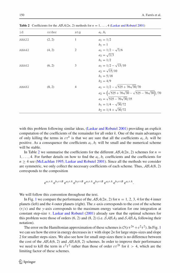
Table 2 Coefficients for the ABA(2n, 2) methods for n = 1, . . . , 4 (Laskar and Robutel 2001)
id order stg ai , bi
ABA22 (2, 2) 1 a1 = 1/2
b1 = 1
ABA42 (4, 2) 2 a1 = 1/2 − √3/6
a2 = √3/3
b1 = 1/2
ABA62 (6, 2) 3 a1 = 1/2 − √15/10
a2 = √15/10
b1 = 5/18
b2 = 4/9
ABA82 (8, 2) 4 a1 = 1/2 −√
525 + 70√
30/70
a2 =(√
525 + 70√
30 −√
525 − 70√
30)/70
a3 =√
525 − 70√
30/35
b1 = 1/4 − √30/72
b2 = 1/4 + √30/72
with this problem following similar ideas, (Laskar and Robutel 2001) providing an explicitcomputation of the coefficients of the remainder for all order k. One of the main advantagesof only killing the terms in ετ k is that we are sure that all the coefficients ai , bi will bepositive. As a consequence the coefficients ai , bi will be small and the numerical schemewill be stable.
In Table 2 we summarise the coefficients for the different ABA(2n, 2) schemes for n =1, . . . , 4. For further details on how to find the ai , bi coefficients and the coefficients forn ≥ 4 see (McLachlan 1995; Laskar and Robutel 2001). Since all the methods we considerare symmetric, we only collect the necessary coefficients of each scheme. Thus, ABA(8, 2)corresponds to the composition
ea1τ A eb1ετ B ea2τ A eb2ετ B ea3τ A eb2ετ B ea2τ A eb1ετ B ea1τ A.
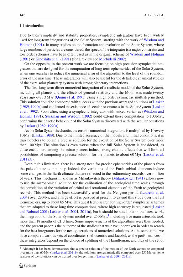
We will follow this convention throughout the text.In Fig. 1 we compare the performance of the ABA(2n, 2) for n = 1, 2, 3, 4 for the 4 inner
planets (left) and the 4 outer planets (right). The x-axis corresponds to the cost of the scheme(τ/s) and the y-axis corresponds to the maximum energy variation for one integration atconstant step-size τ . Laskar and Robutel (2001) already saw that the optimal schemes forthis problem were those of orders (6, 2) and (8, 2) (i.e. SABA3 and SABA4 following theirnotation).
The error on the Hamiltonian approximation of these schemes is O(ετ 2n +ε2τ 2). In Fig. 1we can see how the error in energy decreases in τ with slope 2n for large steps-sizes and slope2 for smaller steps-sizes. We also see how for small step-sizes there is no difference betweenthe cost of the ABA(6, 2) and ABA(8, 2) schemes. In order to improve their performancewe need to kill the term in ε2τ 2 rather than those of order ετ 2k for k > 4, which are thelimiting factor of these schemes.
123

High precision symplectic integrators 151
-18
-16
-14
-12
-10
-8
-6
-4
-5 -4 -3 -2 -1 0
Mer - Ven - Ear - Mar (Jacobi Coord)
ABA22ABA42ABA62ABA82
-18
-16
-14
-12
-10
-8
-6
-4
-5 -4 -3 -2 -1 0
Jup - Sat - Ura - Nep (Jacobi Coord)
ABA22ABA42ABA62ABA82
Fig. 1 Comparison between the ABA(2n, 2) methods for n = 1, 2, 3, 4 applied to the 4 inner planets (left)and the fou outer planets (right). The x-axis represents the cost (τ/s) and the y-axis is the maximum energyvariation over one integration with constant step-size τ . Here s is the number of stages (decimal log scales)
5.2 ABA schemes of order (2n, 4)
In this section we will describe three different procedures to cancel the dominant term ε2τ 2
in order to get methods of generalized order (2n, 4), and discuss their performance for thedifferent test models described in Sect. 4.
5.2.1 The corrector term (SC)
Since in Jacobi coordinates A is quadratic in p and B depends only on q , then it followsthat the term [[A, B], B] depends only on q and thus exp(τ 3ε2[[A, B], B]) can be easilycomputed. Laskar and Robutel (2001) noticed that it is possible to incorporate this term intothe previous compositions with a conveniently chosen constant so as to cancel the term oforder ε2τ 2 in the asymptotic expansion Eq. 15. We note that this corrector scheme is differentthan the one introduced by Wisdom et al. (1996) where the corrector added at the beginningand at the end of each step-size is a change of variables.
Thus, let Sn(τ ) be one of the symplectic ABA schemes of order (2n, 2) described inSect. 5.1. We can get rid of the term in ε2τ 2 by considering
SCn(τ ) = exp(−τ 3ε2 c
2[[A, B], B]
)Sn(τ ) exp
(−τ 3ε2 c
2[[A, B], B]
), (19)
with the appropriate choice of the constant c. In Table 3 we show the value for the coefficientc for each of the 4 ABA(2n, 2) schemes described before. For further details see Laskar and
123
152 A. Farrés et al.
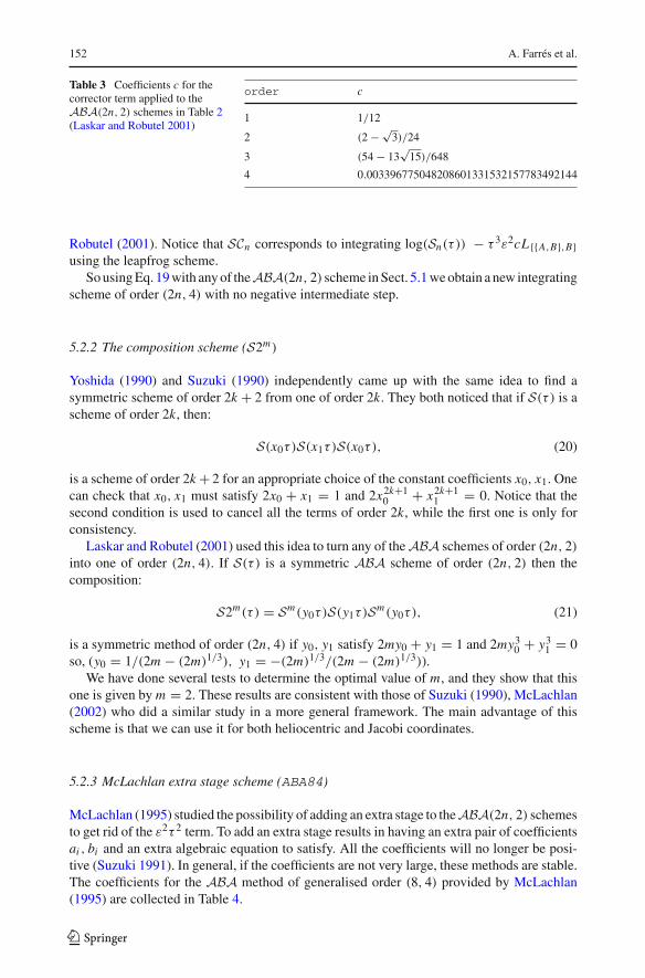
Table 3 Coefficients c for thecorrector term applied to theABA(2n, 2) schemes in Table 2(Laskar and Robutel 2001)
order c
1 1/12
2 (2 − √3)/24
3 (54 − 13√
15)/648
4 0.003396775048208601331532157783492144
Robutel (2001). Notice that SCn corresponds to integrating log(Sn(τ )) − τ 3ε2cL{{A,B},B}using the leapfrog scheme.
So using Eq. 19 with any of theABA(2n, 2) scheme in Sect. 5.1 we obtain a new integratingscheme of order (2n, 4) with no negative intermediate step.
5.2.2 The composition scheme (S2m)
Yoshida (1990) and Suzuki (1990) independently came up with the same idea to find asymmetric scheme of order 2k + 2 from one of order 2k. They both noticed that if S(τ ) is ascheme of order 2k, then:
S(x0τ)S(x1τ)S(x0τ), (20)
is a scheme of order 2k + 2 for an appropriate choice of the constant coefficients x0, x1. Onecan check that x0, x1 must satisfy 2x0 + x1 = 1 and 2x2k+1
0 + x2k+11 = 0. Notice that the
second condition is used to cancel all the terms of order 2k, while the first one is only forconsistency.
Laskar and Robutel (2001) used this idea to turn any of the ABA schemes of order (2n, 2)into one of order (2n, 4). If S(τ ) is a symmetric ABA scheme of order (2n, 2) then thecomposition:
S2m(τ ) = Sm(y0τ)S(y1τ)Sm(y0τ), (21)
is a symmetric method of order (2n, 4) if y0, y1 satisfy 2my0 + y1 = 1 and 2my30 + y3
1 = 0so, (y0 = 1/(2m − (2m)1/3), y1 = −(2m)1/3/(2m − (2m)1/3)).
We have done several tests to determine the optimal value of m, and they show that thisone is given by m = 2. These results are consistent with those of Suzuki (1990), McLachlan(2002) who did a similar study in a more general framework. The main advantage of thisscheme is that we can use it for both heliocentric and Jacobi coordinates.
5.2.3 McLachlan extra stage scheme (ABA84)
McLachlan (1995) studied the possibility of adding an extra stage to the ABA(2n, 2) schemesto get rid of the ε2τ 2 term. To add an extra stage results in having an extra pair of coefficientsai , bi and an extra algebraic equation to satisfy. All the coefficients will no longer be posi-tive (Suzuki 1991). In general, if the coefficients are not very large, these methods are stable.The coefficients for the ABA method of generalised order (8, 4) provided by McLachlan(1995) are collected in Table 4.
123

High precision symplectic integrators 153
Table 4 Coefficients for the ABA method of order (8, 4) found by McLachlan (1995)
id order stg ai , bi
ABA84 (8, 4) 5 a1 = 0.075346960269892888416527803683474464372652667
a2 = 0.51791685468825678230077397849631564432384744
a3 = −0.093263814958149670717301782179790108696500110b1 = 0.19022593937367661924523076273845389746120362
b2 = 0.84652407044352625705508054464677583417711374
b3 = −1.07350001963440575260062261477045946327663472
-18
-16
-14
-12
-10
-8
-6
-5 -4 -3 -2 -1
ABA82S2m m=2
SCABA84
-18
-16
-14
-12
-10
-8
-6
-5 -4 -3 -2 -1
ABA82S2m m=2
SCABA84
-18
-16
-14
-12
-10
-8
-6
-5 -4 -3 -2 -1
ABA82S2m m=2
SCABA84
Mer - Ven - Ear - Mar (Jacobi Coord)
Jup - Sat - Ura - Nep (Jacobi Coord)
Mercury to Neptune (Jacobi Coord)
Fig. 2 Comparison between the different schemes to kill the the ε2τ2 terms in the ABA82 scheme. From leftto right the 4 inner planets, the 4 outer planets and the whole Solar System. The x-axis represents the cost(τ/s) and the y-axis the maximum energy variation for one integration with constant step-size τ (decimal logscales)
5.2.4 Results
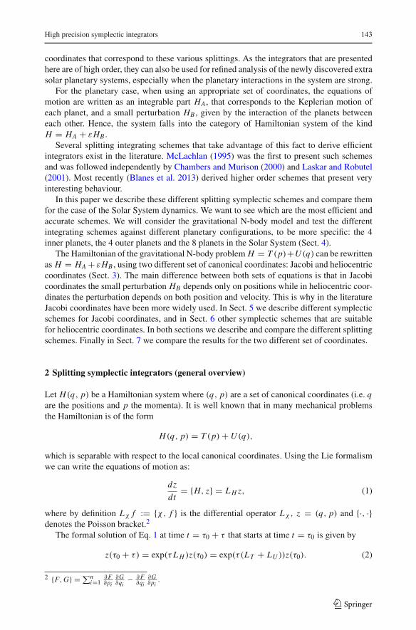
In Fig. 2 we compare the performance of these three different approaches to build methodsof generalised order (8, 4) against the ABA(8, 2) scheme (also referred to as ABA82). In theplots we show the cost (τ/s) versus the maximum energy variation for the three test models:the 4 inner planets (left), the 4 outer planets (middle) and the 8 planets in the Solar System(right).
As we can see, the three different schemes improve considerably the performance ofthe ABA82 (red line). In all cases the corrector scheme SC (blue line) and the McLach-lan ABA84 (purple line) show a similar quantitative behaviour. The difference betweenthem is the cost of the extra stage in ABA84, as we are assuming that the corrector iscompletely free. We note that this is not entirely true if the number of bodies is large(n ≥ 4). On the other hand, the composition methods, S2m (green line), improves theperformance with respect to the ABA82 (red line) but is much more expensive than the othertwo schemes.
123

154 A. Farrés et al.
5.3 ABA schemes with generalised order (s1, s2, . . .)
In the previous section we have seen that adding an extra stage to cancel the term of orderε2τ 2 gives good results. We can extend this idea and add more stages to kill the error termsaccounting to the main limiting factor for each problem (Blanes et al. 2013). This translatesinto adding more constraints on the coefficients. As long as the increase in the computationalcost is less than the gain in accuracy these methods will be competitive. In Fig. 2 we see that thedominant error term for the ABA84 scheme varies between the different test models. Noticethat for the outer planetary system the scheme behaves as one of order 4, so the dominantterm is ε2τ 4. On the other hand, for the inner planetary system, the method behaves as oneof order 8, now the dominant term is ετ 8.
Hence, to improve the performance of the McLachlan’s ABA84 method we need to killdifferent error terms depending on the problem. For the inner planets, a method of order(10, 4) should perform better than one of order (8, 6). While for the outer planets a methodof order (8, 6) should give better results than one of order (10, 4).
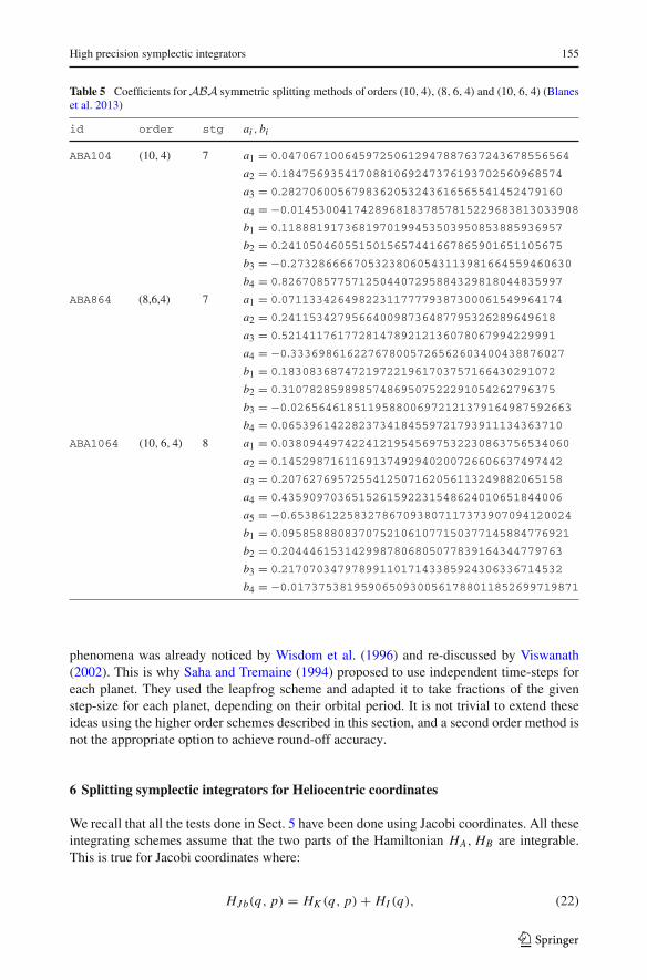
In Blanes et al. (2013) we find details on how to solve the algebraic equations and find theset of coefficients ai , bi that provide ABA schemes for a given arbitrary order (s1, s2, . . .).We must mention that there is no unique combination of coefficients ai , bi for a given order.From all the possible solutions we have selected those that give a better approximation andwhose coefficients ai , bi are small. In Table 5 we summarise the coefficients for three ABAschemes: one of order (10, 4); one of order (8, 6, 4) and one of order (10, 6, 4).
5.3.1 Results
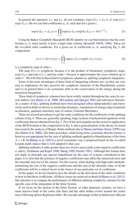
In Fig. 3 we compare the performance of the three schemes summarised in Table 5 againstthe ABA82 and ABA84 for the three test models.
In the left-hand side of Fig. 3 we have the results for the 4 inner planets. We recall that thedominant error term in the ABA84 scheme was ετ 8. Hence, a method of order 10 in ε shouldperform better than one of order 8 in ε. Nevertheless, as we can see there is no significant gainin the performance of these schemes with respect to ABA84. Apparently, for these methodsthe gain in precision is proportional to the computational cost in this range of accuracy.
In the middle of Fig. 3 we have the results for the 4 outer planets. We recall that herethe dominant term in the ABA84 scheme was ε2τ 4, hence we expect the schemes of order 6in ε2 to be better than the ABA84. As we can see the ABA864 and the ABA1064 schemesgive better results that the ABA84. In both cases the optimal cost is around 10−2 versus anoptimal cost of around 10−3 for the ABA84 scheme.
The main difference between the inner planets and the outer planets is the size of theperturbation. We recall that in Jacobi coordinates, for the inner planets ε ≈ 4.54 · 10−6,while for the outer planets ε ≈ 2.03 · 10−4 (see Table 1). The difference of about 2 ordersof magnitude should explain the difference in the performance of the different schemes,as the relevance of the terms εiτ 2k in the error approximation will vary depending on thesize of ε.
Taking this into account, one can be surprised by the performance of these schemeswhen we consider the whole Solar System (Fig. 3 right). Here the size of the perturbation(ε ≈ 1.96 · 10−4) is of the same order of magnitude as the case of the outer planets. But aswe can see in Fig. 3 the schemes behave in the same way as the case of the inner planets,where the terms of order ετ 8 dominate those of order ε2τ 4. We think this is due to Mercury:its fast orbital period and large eccentricity is limiting the performance of the methods. This
123
High precision symplectic integrators 155
Table 5 Coefficients for ABA symmetric splitting methods of orders (10, 4), (8, 6, 4) and (10, 6, 4) (Blaneset al. 2013)
id order stg ai , bi
ABA104 (10, 4) 7 a1 = 0.04706710064597250612947887637243678556564
a2 = 0.1847569354170881069247376193702560968574
a3 = 0.2827060056798362053243616565541452479160
a4 = −0.01453004174289681837857815229683813033908b1 = 0.1188819173681970199453503950853885936957
b2 = 0.2410504605515015657441667865901651105675
b3 = −0.2732866667053238060543113981664559460630b4 = 0.8267085775712504407295884329818044835997
ABA864 (8,6,4) 7 a1 = 0.0711334264982231177779387300061549964174
a2 = 0.241153427956640098736487795326289649618
a3 = 0.521411761772814789212136078067994229991
a4 = −0.333698616227678005726562603400438876027b1 = 0.183083687472197221961703757166430291072
b2 = 0.310782859898574869507522291054262796375
b3 = −0.0265646185119588006972121379164987592663b4 = 0.0653961422823734184559721793911134363710
ABA1064 (10, 6, 4) 8 a1 = 0.03809449742241219545697532230863756534060
a2 = 0.1452987161169137492940200726606637497442
a3 = 0.2076276957255412507162056113249882065158
a4 = 0.4359097036515261592231548624010651844006
a5 = −0.6538612258327867093807117373907094120024b1 = 0.09585888083707521061077150377145884776921
b2 = 0.2044461531429987806805077839164344779763
b3 = 0.2170703479789911017143385924306336714532
b4 = −0.01737538195906509300561788011852699719871
phenomena was already noticed by Wisdom et al. (1996) and re-discussed by Viswanath(2002). This is why Saha and Tremaine (1994) proposed to use independent time-steps foreach planet. They used the leapfrog scheme and adapted it to take fractions of the givenstep-size for each planet, depending on their orbital period. It is not trivial to extend theseideas using the higher order schemes described in this section, and a second order method isnot the appropriate option to achieve round-off accuracy.
6 Splitting symplectic integrators for Heliocentric coordinates
We recall that all the tests done in Sect. 5 have been done using Jacobi coordinates. All theseintegrating schemes assume that the two parts of the Hamiltonian HA, HB are integrable.This is true for Jacobi coordinates where:
HJb(q, p) = HK (q, p)+ HI (q), (22)
123
156 A. Farrés et al.
-18
-16
-14
-12
-10
-8
-6
-5 -4 -3 -2 -1
ABA82ABA84
ABA104ABA864
ABA1064
-18
-16
-14
-12
-10
-8
-6
-5 -4 -3 -2 -1
ABA82ABA84
ABA104ABA864
ABA1064
-18
-16
-14
-12
-10
-8
-6
-5 -4 -3 -2 -1
ABA82ABA84
ABA104ABA864
ABA1064
Mer - Ven - Ear - Mar (Jacobi Coord)
Jup - Sat - Ura - Nep (Jacobi Coord) [ short ]
Mercury to Neptune (Jacobi Coord)
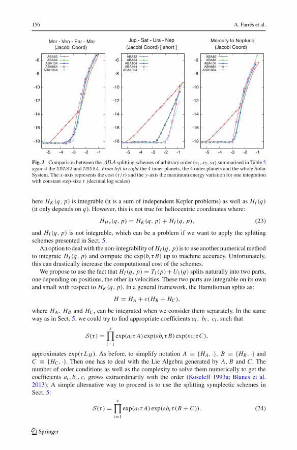
Fig. 3 Comparison between the ABA splitting schemes of arbitrary order (s1, s2, s3) summarised in Table 5against the ABA82 and ABA84. From left to right the 4 inner planets, the 4 outer planets and the whole SolarSystem. The x-axis represents the cost (τ/s) and the y-axis the maximum energy variation for one integrationwith constant step-size τ (decimal log scales)
here HK (q, p) is integrable (it is a sum of independent Kepler problems) as well as HI (q)(it only depends on q). However, this is not true for heliocentric coordinates where:
HHe(q, p) = HK (q, p)+ HI (q, p), (23)
and HI (q, p) is not integrable, which can be a problem if we want to apply the splittingschemes presented in Sect. 5.
An option to deal with the non-integrability of HI (q, p) is to use another numerical methodto integrate HI (q, p) and compute the exp(biτ B) up to machine accuracy. Unfortunately,this can drastically increase the computational cost of the schemes.
We propose to use the fact that HI (q, p) = T1(p)+ U1(q) splits naturally into two parts,one depending on positions, the other in velocities. These two parts are integrable on its ownand small with respect to HK (q, p). In a general framework, the Hamiltonian splits as:
H = HA + ε(HB + HC ),
where HA, HB and HC , can be integrated when we consider them separately. In the sameway as in Sect. 5, we could try to find appropriate coefficients ai , bi , ci , such that
S(τ ) =s∏
i=1
exp(aiτ A) exp(εbiτ B) exp(εciτC),
approximates exp(τ L H ). As before, to simplify notation A ≡ {HA, ·}, B ≡ {HB , ·} andC ≡ {HC , ·}. Then one has to deal with the Lie Algebra generated by A, B and C . Thenumber of order conditions as well as the complexity to solve them numerically to get thecoefficients ai , bi , ci grows extraordinarily with the order (Koseleff 1993a; Blanes et al.2013). A simple alternative way to proceed is to use the splitting symplectic schemes inSect. 5:
S(τ ) =s∏
i=1
exp(aiτ A) exp(εbiτ(B + C)). (24)
123

High precision symplectic integrators 157
-18
-16
-14
-12
-10
-8
-6
-5 -4 -3 -2 -1
ABA 82S2m m=2
ABA 84
-18
-16
-14
-12
-10
-8
-6
-5 -4 -3 -2 -1
ABA 82S2m m=2
ABA 84
-18
-16
-14
-12
-10
-8
-6
-5 -4 -3 -2 -1
ABA 82S2m m=2
ABA 84
Mer - Ven - Ear - Mar (Helio Coord)
Jup - Sat - Ura - Nep (Helio Coord)
Mercury to Neptune (Helio Coord)
Fig. 4 Comparison between the ABA82, ABA84 and S2m schemes discussed in Sect. 5.2 applied to helio-centric coordinates. From left to right the 4 inner planets, the 4 outer planets and the whole Solar System.The x-axis represents the cost (τ/s) and the y-axis the maximum energy variation for one integration withconstant step-size τ (decimal log scales)
and approximate exp(εbiτ(B + C)) with
exp(εbiτ(B + C)) ≈ exp
(
εbi
2τC
)
exp(εbiτ B) exp
(
εbi
2τC
)
. (25)
Here we take C as the Lie operator associated to T1(p) due to its lower computational cost.In general HB and HC do not commute ({HB , HC } �= 0), so this approximation adds an
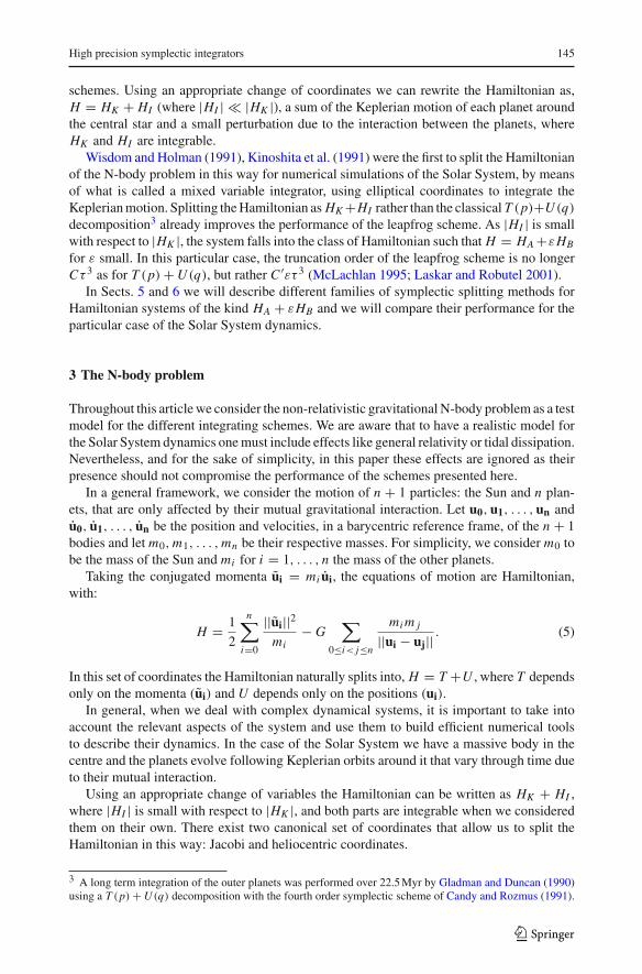
extra error contribution term, ε3τ 2, which will be negligible for small ε. In Fig. 4 we see theresult of taking the ABA82, the ABA84 and the S2m splitting schemes using Eq. 25 to dealwith heliocentric coordinates. We can see that in general the symplectic schemes have thesame behaviour as with Jacobi coordinates (Fig. 2).
We do see a difference in the case of the outer planets (Fig. 4 middle). Now the ABA84scheme behaves as one of order 2 for small step-sizes. This is due to the extra error termε3τ 2. We recall that the main difference between the inner and the outer planets is the sizeof the perturbation (ε) which is smaller in the first case. Here the terms of order ε3τ 2 arenegligible for the inner planets but not for the outer planets.
Unfortunately, when we consider high-order symplectic schemes like the ones presentedin Sect. 5.3 these extra error terms will become relevant, jeopardising the performance ofthese schemes.
The first symplectic schemes using heliocentric coordinates (Koseleff 1993a; Touma andWisdom 1994) used the form of heliocentric Hamiltonian where the unperturbed problem isthe Keplerian motion of a planet around the Sun as in Laskar (1991), Laskar (1990b). Lateron Duncan et al. (1998) proposed to rewrite the Hamiltonian in heliocentric variables forwhich the unperturbed problem is the Keplerian motion of a planet around a fixed Sun. Forthis decomposition, the unperturbed Keplerian approximation is less accurate (see Duncanet al. 1998), but HB and HC commute ({HB , HC } = 0), and thus exp(εbiτ(B + C)) =exp(εbiτ B) exp(εbiτC). For further details see Appendix C.
123

158 A. Farrés et al.
Table 6 Coefficients for ABAH specific symmetric splitting methods for heliocentric coordinates of orders(8, 4), (8, 6, 4) and (10, 6, 4) (Blanes et al. 2013)
id order stg ai , bi
ABAH844 (8, 4) 6 a1 = 0.2741402689434018761640565440378637101205
a2 = −0.1075684384401642306251105297063236526845a3 = −0.04801850259060169269119541715084750653701a4 = 0.7628933441747280943044988056386148982021
b1 = 0.6408857951625127177322491164716010349386
b2 = −0.8585754489567828565881283246356000103664b3 = 0.7176896537942701388558792081639989754277
ABAH864 (8, 6, 4) 8 a1 = 0.06810235651658372084723976682061164571212
a2 = 0.2511360387221033233072829580455350680082
a3 = −0.07507264957216562516006821767601620052338a4 = −0.009544719701745007811488218957217113269121a5 = 0.5307579480704471776340674235341732001443
b1 = 0.1684432593618954534310382697756917558148
b2 = 0.4243177173742677224300351657407231801453
b3 = −0.5858109694681756812309015355404036521923b4 = 0.4930499927320125053698281000239887162321
ABAH1064 (10, 6, 4) 9 a1 = 0.04731908697653382270404371796320813250988
a2 = 0.2651105235748785159539480036185693201078
a3 = −0.009976522883811240843267468164812380613143a4 = −0.05992919973494155126395247987729676004016a5 = 0.2574761120673404534492282264603316880356
b1 = 0.1196884624585322035312864297489892143852
b2 = 0.3752955855379374250420128537687503199451
b3 = −0.4684593418325993783650820409805381740605b4 = 0.3351397342755897010393098942949569049275
b5 = 0.2766711191210800975049457263356834696055
6.1 ABAH schemes of order (2n, 4) specific for heliocentric coordinates
We have just seen that for heliocentric coordinates we can adapt the splitting schemesdescribed is Sect. 5 using Eqs. 24 and 25. But with this an extra term ε3τ 2 appears inthe error approximation that will limit the performance for high-order schemes. One cancheck that this error term is associated to the algebraic expression b3
1 + b32 + · · · + b3
n . Wecan add an extra stage to the scheme so that it also satisfies:
b31 + b3
2 + · · · + b3n = 0,
leading to symplectic schemes with the same generalised order as before for heliocentriccoordinates. Table 6 collects the coefficients for the ABAH scheme of order (8, 4) forheliocentric coordinates. This scheme has the same effective order as the McLachlan ABAscheme of order (8, 4) (Sect. 5.2.3) but it is specific for heliocentric coordinates. In Fig. 5we compare the performance of this new scheme against the ABA84 scheme. As we can see,
123
High precision symplectic integrators 159
-18
-16
-14
-12
-10
-8
-6
-5 -4 -3 -2 -1
ABA 84ABAH 844
-18
-16
-14
-12
-10
-8
-6
-5 -4 -3 -2 -1
ABA 84ABAH 844
-18
-16
-14
-12
-10
-8
-6
-5 -4 -3 -2 -1
ABA 84ABAH 844
Mer - Ven - Ear - Mar (Helio Coord)
Jup - Sat - Ura - Nep (Helio Coord)
Mercury to Neptune (Helio Coord)
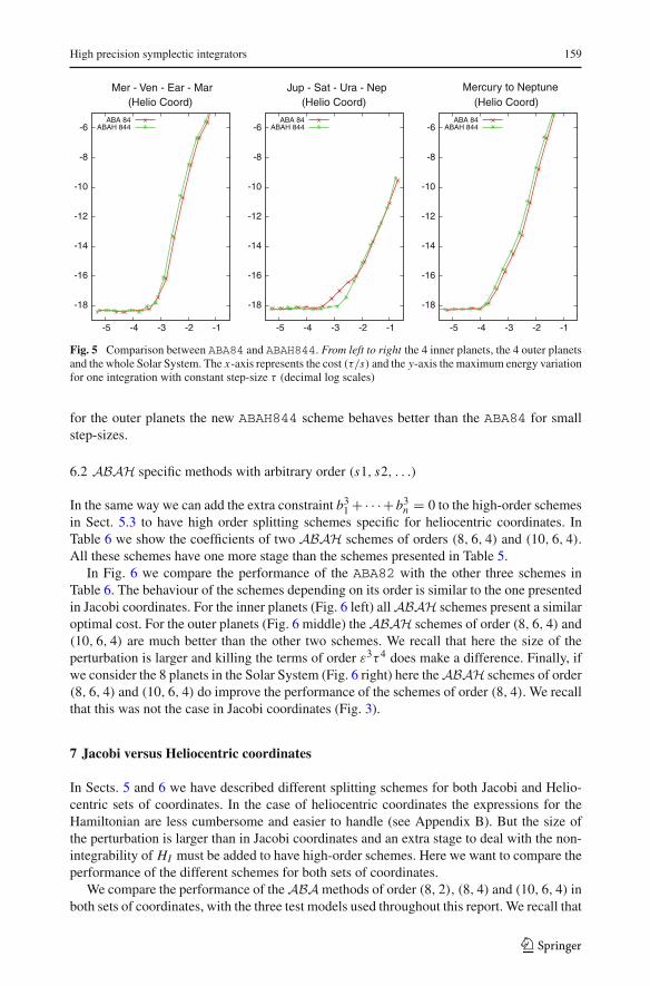
Fig. 5 Comparison between ABA84 and ABAH844. From left to right the 4 inner planets, the 4 outer planetsand the whole Solar System. The x-axis represents the cost (τ/s) and the y-axis the maximum energy variationfor one integration with constant step-size τ (decimal log scales)
for the outer planets the new ABAH844 scheme behaves better than the ABA84 for smallstep-sizes.
6.2 ABAH specific methods with arbitrary order (s1, s2, . . .)
In the same way we can add the extra constraint b31 +· · ·+b3
n = 0 to the high-order schemesin Sect. 5.3 to have high order splitting schemes specific for heliocentric coordinates. InTable 6 we show the coefficients of two ABAH schemes of orders (8, 6, 4) and (10, 6, 4).All these schemes have one more stage than the schemes presented in Table 5.
In Fig. 6 we compare the performance of the ABA82 with the other three schemes inTable 6. The behaviour of the schemes depending on its order is similar to the one presentedin Jacobi coordinates. For the inner planets (Fig. 6 left) all ABAH schemes present a similaroptimal cost. For the outer planets (Fig. 6 middle) the ABAH schemes of order (8, 6, 4) and(10, 6, 4) are much better than the other two schemes. We recall that here the size of theperturbation is larger and killing the terms of order ε3τ 4 does make a difference. Finally, ifwe consider the 8 planets in the Solar System (Fig. 6 right) here the ABAH schemes of order(8, 6, 4) and (10, 6, 4) do improve the performance of the schemes of order (8, 4). We recallthat this was not the case in Jacobi coordinates (Fig. 3).
7 Jacobi versus Heliocentric coordinates
In Sects. 5 and 6 we have described different splitting schemes for both Jacobi and Helio-centric sets of coordinates. In the case of heliocentric coordinates the expressions for theHamiltonian are less cumbersome and easier to handle (see Appendix B). But the size ofthe perturbation is larger than in Jacobi coordinates and an extra stage to deal with the non-integrability of HI must be added to have high-order schemes. Here we want to compare theperformance of the different schemes for both sets of coordinates.
We compare the performance of the ABA methods of order (8, 2), (8, 4) and (10, 6, 4) inboth sets of coordinates, with the three test models used throughout this report. We recall that
123
160 A. Farrés et al.
-18
-16
-14
-12
-10
-8
-6
-5 -4 -3 -2 -1
ABA 82ABAH 844ABAH 864
ABAH 1064
-18
-16
-14
-12
-10
-8
-6
-5 -4 -3 -2 -1
ABA 82ABAH 844ABAH 864
ABAH 1064
-18
-16
-14
-12
-10
-8
-6
-5 -4 -3 -2 -1
ABA 82ABAH 844ABAH 864
ABAH 1064
Mercury to Neptune (Helio Coord)
Jup - Sat - Ura - Nep (Helio Coord)
Mer - Ven - Ear - Mar (Helio Coord)
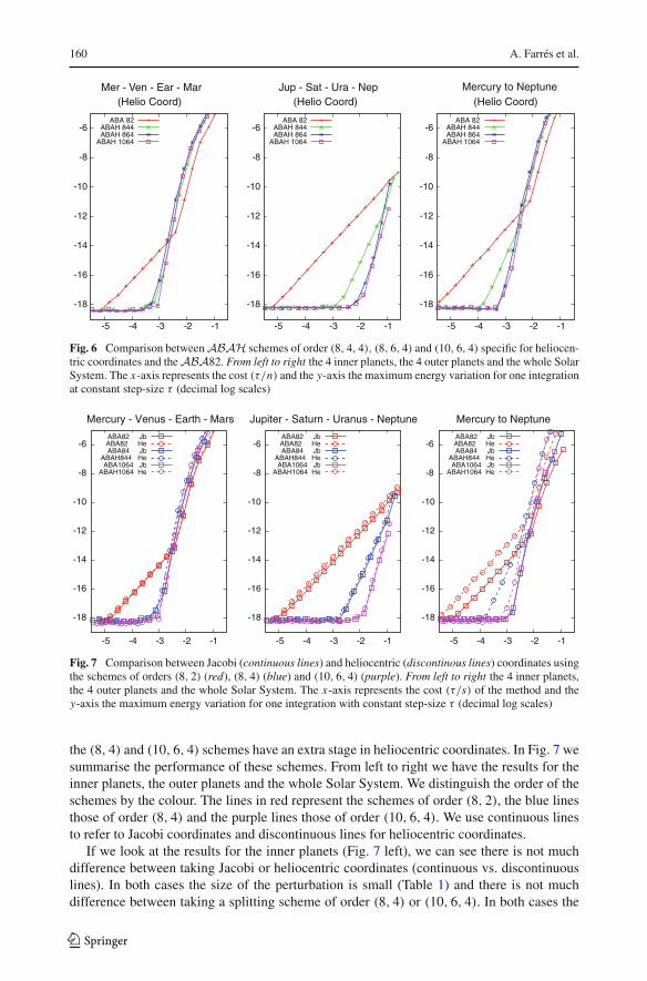
Fig. 6 Comparison between ABAH schemes of order (8, 4, 4), (8, 6, 4) and (10, 6, 4) specific for heliocen-tric coordinates and the ABA82. From left to right the 4 inner planets, the 4 outer planets and the whole SolarSystem. The x-axis represents the cost (τ/n) and the y-axis the maximum energy variation for one integrationat constant step-size τ (decimal log scales)
-18
-16
-14
-12
-10
-8
-6
-5 -4 -3 -2 -1
Mercury - Venus - Earth - Mars
ABA82 JbABA82 HeABA84 Jb
ABAH844 HeABA1064 Jb
ABAH1064 He
-18
-16
-14
-12
-10
-8
-6
-5 -4 -3 -2 -1
Jupiter - Saturn - Uranus - Neptune
ABA82 JbABA82 HeABA84 Jb
ABAH844 HeABA1064 Jb
ABAH1064 He
-18
-16
-14
-12
-10
-8
-6
-5 -4 -3 -2 -1
Mercury to Neptune
ABA82 JbABA82 HeABA84 Jb
ABAH844 HeABA1064 Jb
ABAH1064 He
Fig. 7 Comparison between Jacobi (continuous lines) and heliocentric (discontinous lines) coordinates usingthe schemes of orders (8, 2) (red), (8, 4) (blue) and (10, 6, 4) (purple). From left to right the 4 inner planets,the 4 outer planets and the whole Solar System. The x-axis represents the cost (τ/s) of the method and they-axis the maximum energy variation for one integration with constant step-size τ (decimal log scales)
the (8, 4) and (10, 6, 4) schemes have an extra stage in heliocentric coordinates. In Fig. 7 wesummarise the performance of these schemes. From left to right we have the results for theinner planets, the outer planets and the whole Solar System. We distinguish the order of theschemes by the colour. The lines in red represent the schemes of order (8, 2), the blue linesthose of order (8, 4) and the purple lines those of order (10, 6, 4). We use continuous linesto refer to Jacobi coordinates and discontinuous lines for heliocentric coordinates.
If we look at the results for the inner planets (Fig. 7 left), we can see there is not muchdifference between taking Jacobi or heliocentric coordinates (continuous vs. discontinuouslines). In both cases the size of the perturbation is small (Table 1) and there is not muchdifference between taking a splitting scheme of order (8, 4) or (10, 6, 4). In both cases the
123
High precision symplectic integrators 161
terms in ε in the error expansion are the ones that matter, but there is not much differencebetween taking order 8 or ten in ετ k . We should have to use arithmetics with higher precisionto see the difference (see Appendix D). Hence the ABA84 is the best choice for this case.
If we look at the results for the outer planets (Fig. 7 middle), again there is no significantdifference between Jacobi and heliocentric coordinates. But here the ABA schemes of order(10, 6, 4) perform much better that the other schemes, having an optimal step-size one orderof magnitude larger than the ones for the schemes of order (8, 4).
If we look at the whole Solar System (Fig. 7 right), we see that there is a big differencebetween taking Jacobi or heliocentric coordinates. Looking at the ABA82 scheme (red lines)we see that the slopes are the same but that there is a difference of about one order ofmagnitude in accuracy for a given step-sizes. If we look at the scheme of order (8, 4) (bluelines), we see that in Jacobi coordinates the methods behave as one of order 8, while inheliocentric coordinates this one behaves as one of order 4. This can be explained by thedifference in the size of the perturbation (see Table 1) in both set of coordinates. We alsosee that there is a big difference between the optimal step-size for both sets of coordinates,making Jacobi coordinates by far the best choice. Finally, if we compare the ABA schemes oforder (10, 6, 4) (purple lines) the difference between the two set of coordinates is drasticallyreduced, although Jacobi coordinates still perform slightly better. However, the extra stagesto go from an (8, 4) scheme to a (10, 6, 4) one do not improve in Jacobi coordinates. Thisis not the case of heliocentric coordinates, where the (10, 6, 4) gives the best results and thedifference between the two set of coordinates is not as relevant as before.
To sum up, we recommend to use either the schemes ABA84or ABA1064 in the case ofJacobi coordinates, while for heliocentric coordinates one should use theABAH1064 scheme.Although Jacobi coordinates present slightly better results for most of the test models, webelieve that using Jacobi or heliocentric coordinates is a matter of choice.
8 Conclusions
In this article we have reviewed different symplectic splitting schemes and tested their per-formance for the case of the planetary motion, focussing on the Solar System motion. Werecall that in the case of the planetary motion, using an appropriate change of variables, theHamiltonian of the N-body problem can be rewritten as HK + HI . A sum of independentKeplerian motions for each planet (HK ) and a small perturbation term given by the interactionbetween the planets (HI ).
There are two set of canonical coordinates that allow us to write the Hamiltonian in thisway: Jacobi and heliocentric coordinates (Sect. 3). Although in Jacobi coordinates the size ofthe perturbation is smaller and HI is integrable, heliocentric coordinates seem more naturaland the expressions are easier to handle (Appendix B). In this article we have compared theperformance of different symplectic splitting schemes in both sets of coordinates.
In Sect. 5 we described different splitting symplectic schemes for Jacobi coordinates. InSect. 6 we saw how to extend these schemes to use heliocentric coordinates. We note thatall the splitting schemes for Jacobi coordinates can also be used in Heliocentric coordinates,but in order to have a comparable performance an extra stage to kill the terms in ε3τ 2 mustbe added (see Sect. 6).
We have seen that in Jacobi coordinates, the ABA84 scheme introduced by McLachlan(1995) and the ABA1064 scheme (Blanes et al. 2013) give the best results when we look atthe motion of the whole Solar System. The high eccentricity of Mercury and its fast orbitalperiod are the main limiting factors and taking higher order splitting schemes do not always
123

162 A. Farrés et al.
provide significant improvements. But for different planetary configurations, as the 4 outerplanets, the ABA1064 scheme has a better performance than the ABA84 method.
When we consider heliocentric coordinates, the ABAH1064 method (Blanes et al. 2013)gives the best results when we consider the whole Solar System. In this case, probably becausethe size of the perturbation is larger, adding extra stages to have higher order schemes doesimprove the results. The nominal solution La2010a of Laskar et al. (2011a) was computedwith the ABA82 scheme and a stepsize of 10−3 yr. Using the ABAH1064 scheme, the sameaccuracy should be reached with nearly an order of magnitude improvement in the comput-ing time (Fig. 6). The performances of the schemes in both sets of coordinates, Jacobi orheliocentric are very similar for the scheme of order (10, 6, 4), with a slight advantage forthe Jacobi coordinates. Depending on the problem, one can thus use either system of coor-dinates, but it is clear that using high order schemes as the ABA(H)864 and ABA(H)1064(Blanes et al. 2013) can drastically improve the results. This should be even more the case forhighly perturbed systems as some extra solar planetary systems with close planets of largemasses and large eccentricities. It should be nevertheless noted that although these high orderintegrators behave well until very large eccentricities (up to 0.99 in some of our simulations),some specific integrators need to be used when collisional behaviors are considered (Duncanet al. 1998; Chambers 1999).
Acknowledgements This work was supported by GTSNext project. The work of SB, FC, JM and AM hasbeen partially supported by Ministerio de Ciencia e Innovación (Spain) under project MTM2010-18246-C03(co-financed by FEDER Funds of the European Union).
Appendix A: On the compensated summation
Using any of the symplectic integrating schemes described in this article, we require succes-sive evaluations of exp(aiτ A) and exp(biτ B). Each of these evaluations slightly modifiesthe position and velocity of each planet. For τ small, we will have a loss in accuracy due toround-off errors. The Compensated Summation is a simple trick that is commonly used toreduce the round-off error. In a general framework, when we consider a numerical methodfor solving an ODE, we require a recursive evaluation of the form:
yn+1 = yn + δn, (26)
where yn is the approximated solution and δn is the increment to be done. Usually δn will besmaller in magnitude than yn . In this situation, the rounding errors caused by the computationof δn are in general smaller that those to evaluate Eq. 26. The algorithm that can be used inorder to reduce this round-off error is called the “Compensated Summation” (Kahan 1965).
Compensated summation algorithm: Let y0 and {δn}n≥0 be given and put e = 0.Compute y1, y2, . . . from Eq. 26 as follows:
f or n = 0, 1, 2, . . . doa = yn
e = e + δn
yn+1 = a + ee = e + (a − yn+1)
enddo
This algorithm accumulates the rounding errors in e and feeds them back into the sum-mation when possible. At each time-step of the integration, when we evaluate exp(aiτ A) or
123

High precision symplectic integrators 163
-16
-15
-14
-13
-12
-11
-10
-9
-8
-6 -5 -4 -3 -2
Jup - Sat [Double Precisions CS Vs NO CS]
ABA22 CSABA42 CSABA62 CSABA82 CS
ABA22 no CSABA42 no CSABA62 no CSABA82 no CS
-20
-18
-16
-14
-12
-10
-8
-6 -5 -4 -3 -2
Jup - Sat [Extended Precisions CS Vs NO CS]
ABA22 CSABA42 CSABA62 CSABA82 CS
ABA22 no CSABA42 no CSABA62 no CSABA82 no CS
Fig. 8 Comparison between the ABA schemes of order (2n, 2) for n = 1, 2, 3, 4 applied to the Sun-Jupiter-Saturn three body problem. With (CS) and without (noCS) the compensated summation. The x-axis representthe cost (τ/n) and the y-axis the maximum energy variation for one integration with constant step-size τ . Leftusing a double precision arithmetics; Right using an extended precision arithmetics (decimal log scales)
exp(biτ B), the increment in position and velocity is done using the compensated summation.In Fig. 8 we show the results for the ABA(2n, 2) schemes for n = 1, 2, 3, 4 using double(left) and extended precision (right). In both cases we gain almost one order of magnitude inprecision when we take into account the compensated summation.
Appendix B: Integration schemes (some help on the practical coding)
In this paper we have reviewed many splitting symplectic integrating schemes, all of themof the form:
S(τ ) = exp(a1τ A) exp(b1τ B) . . . exp(b1τ B) exp(a1τ A), (27)
where exp(τ A) and exp(τ B) can be computed explicitly. They correspond to the integrals ofthe two different parts of the original Hamiltonian. In this section we show how to computeexplicitly exp(τ A) and exp(τ B) for the particular case of the N-body problem in Jacobi andheliocentric coordinates. We note that from now on: u stands for the momenta associated tou and u′ stands for du/dt .
B.1 Keplerian motion (HK )
We recall that in Jacobi coordinates,
HK =n∑
i=1
(1
2
ηi
ηi−1
||vi||2mi
− Gmiηi−1
||vi||)
, (28)
whereas in heliocentric coordinates,
HK =n∑
i=1
(1
2||ri||2
[m0 + mi
m0mi
]
− Gm0mi
||ri||)
. (29)
In both cases HK is a sum of independent Keplerian motions. In Jacobi coordinates eachplanet follows an elliptical orbit around the centre on mass of the Sun and the planets thatare closer to the Sun, the mass parameter of the system is μJ = Gηi . While in heliocentric
123

164 A. Farrés et al.
coordinates each planet follows an elliptical orbit around the planet-Sun centre of mass, andthe mass parameter of the system is μH = G(m0 + mi ).
It is well known that Kepler problem is integrable, but the solution from time t = t0 tot = t0 + τ is expressed in a simple form if we consider action-angle variables. To computeexp(τ L HK ) we need to be able to compute (r(t0 + τ), v(t0 + τ)) from (r(t0), v(t0)).
An option is to change to elliptical coordinates, advance the mean anomaly and then returnto Cartesian coordinates. But this can accumulate a lot of numerical errors as well as it isvery expensive in terms of computational cost. Instead we use a similar idea as the Gauss fand g functions (Danby 1992), where we use an expression for the increment in position andvelocities for a given step-size τ , without having to perform any change of coordinates. Letus give some details on how to derive these expressions.
In elliptical coordinates the motion of the two body problem is given by (a, e, i,Ω,ω, E),where all of the elements remain fixed except for E that varies following Kepler equation(n(t − tp) = M = E − e sin E). Using a reference frame where the orbital plane is given byZ = 0, the X -axis is the direction of the perihelion and the Y -axis completes an orthogonalreference system on the orbital plane, the position (X, Y, 0) and velocity (X ′, Y ′, 0) aregiven by:
X = a(cos E − e), Y = a√
1 − e2 sin E,
X ′ = −na2
rsin E, Y ′ = na2
r
√1 − e2 cos E,
(30)
where r = a(1−e cos E) and n = μ1/2a−3/2. The position and velocities on a fixed referenceframe are given by:
⎛
⎝x x ′y y′z z′
⎞
⎠ = R3(Ω)× R1(i)× R3(ω)×⎛
⎝X X ′Y Y ′0 0
⎞
⎠ , (31)
where
R1(θ) =⎛
⎝1 0 00 cos θ sin θ0 − sin θ cos θ
⎞
⎠ , and R3(θ) =⎛
⎝cos θ sin θ 0
− sin θ cos θ 00 0 1
⎞
⎠
Notice that
R3(Ω)× R1(i)× R3(ω) = R × R3( ),
where = Ω + ω and R = R3(Ω) × R1(i) × R3(−Ω). Given that R1(i) =R1(i/2)R1(i/2) we have that:
R =⎛
⎝1 − 2p2 2pq 2pχ
2pq 1 − 2q2 −2qχ−2pχ 2qχ 1 − 2p2 − 2q2
⎞
⎠ , (32)
123
High precision symplectic integrators 165
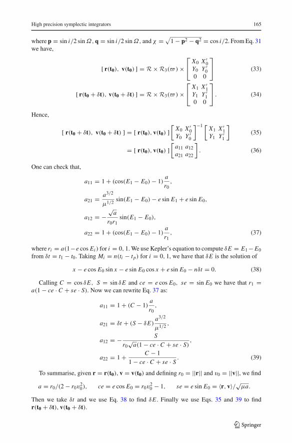
where p = sin i/2 sinΩ,q = sin i/2 sinΩ, andχ = √1 − p2 − q2 = cos i/2. From Eq. 31
we have,
[ r(t0), v(t0) ] = R × R3( )×⎡
⎣X0 X ′
0Y0 Y ′
00 0
⎤
⎦ (33)
[ r(t0 + δt), v(t0 + δt) ] = R × R3( )×⎡
⎣X1 X ′
1Y1 Y ′
10 0
⎤
⎦ . (34)
Hence,
[ r(t0 + δt), v(t0 + δt) ] = [ r(t0), v(t0) ][
X0 X ′0
Y0 Y ′0
]−1 [X1 X ′
1Y1 Y ′
1
]
(35)
= [ r(t0), v(t0) ][
a11 a12
a21 a22
]
. (36)
One can check that,
a11 = 1 + (cos(E1 − E0)− 1)a
r0,
a21 = a3/2
μ1/2 sin(E1 − E0)− e sin E1 + e sin E0,
a12 = −√
a
r0r1sin(E1 − E0),
a22 = 1 + (cos(E1 − E0)− 1)a
r1, (37)
where ri = a(1−e cos Ei ) for i = 0, 1. We use Kepler’s equation to compute δE = E1 − E0
from δt = t1 − t0. Taking Mi = n(ti − tp) for i = 0, 1, we have that δE is the solution of
x − e cos E0 sin x − e sin E0 cos x + e sin E0 − nδt = 0. (38)
Calling C = cos δE, S = sin δE and ce = e cos E0, se = sin E0 we have that r1 =a(1 − ce · C + se · S). Now we can rewrite Eq. 37 as:
a11 = 1 + (C − 1)a
r0,
a21 = δt + (S − δE)a3/2
μ1/2 ,
a12 = − S
r0√
a(1 − ce · C + se · S),
a22 = 1 + C − 1
1 − ce · C + se · S. (39)
To summarise, given r = r(t0), v = v(t0) and defining r0 = ||r|| and v0 = ||v||, we find
a = r0/(2 − r0v20), ce = e cos E0 = r0v
20 − 1, se = e sin E0 = 〈r, v〉/√μa.
Then we take δt and we use Eq. 38 to find δE . Finally we use Eqs. 35 and 39 to findr(t0 + δt), v(t0 + δt).
123

166 A. Farrés et al.
B.2 Jacobi coordinates
We recall that in this set of coordinates the perturbation part is given by:
HI = U1 = G
⎡
⎣n∑
i=1
mi
(ηi−1
||vi|| − m0
||ri||)
−∑
0<i< j≤n
(mi m j
||ri − rj||)
⎤
⎦ . (40)
B.2.1 Computing exp(L HI )
U1 depends only on the position, hence the equations of motion are given by,
d
dtvk = ∂U1
∂ vk,
d
dtvk = −∂U1
∂ vk.
Using vi = ηi−1mi
ηivi we have
vk(τ ) = vk(τ0), vk(τ ) = vk(τ0)− τηi
ηi−1mi
∂U1
∂vk.
As the expressions for ∂U1/∂vk can be a little cumbersome, we compute them separately.When we derive HI with respect to vk we must derive 3 main expressions: 1/||vi||, 1/||ri||and 1/||ri − rj|| for i < j . We first give the derivatives of these factors with respect to vkand then we will deduce ∂HI /∂vk for k = 1, . . . , n.
∂
∂vk
(1
||vi||)
= − vi
||vi||3 · δi,k, where δi,k ={
0 if i �= k,1 if i = k.
∂
∂vk
(1
||ri||)
= − ri
||ri||3 · ξi,k, where ξi,k =
⎧⎪⎨
⎪⎩
0 if i < k,1 if i = k,
mk
ηkif i > k.
∂
∂vk
(1
||ri−rj||)
=− ri−rj
||ri−rj||3 · ψi, j,k, where ψi, j,k =
⎧⎪⎪⎪⎪⎪⎨
⎪⎪⎪⎪⎪⎩
ηk−1
ηkif k = i < j,
−mk
ηkif i < k < j,
−1 if i < j = k,0 else (k< i< j, i< j<k).
To compute ∂U1/∂vk for k = 1, . . . , n, we consider separately the cases k = 1 and k > 1:
∂U1
∂v1= G
m0m1
η1
⎡
⎣n∑
i=2
miri
||ri||3+
n∑
i=2
mir1 − ri
||r1 − ri||3
⎤
⎦ .
∂U1
∂vk= Gmk
⎡
⎣−ηk−1vk
||vk||3 + m0rk
||rk||3 + m0
ηk
n∑
i=k+1
miri
||ri||3
+ ηk−1
ηk
n∑
j=k+1
m jrk−rj
||rk−rj||3−
k−1∑
i=1
miri−rk
||ri−rk||3 − 1
ηk
k−1∑
i=1
n∑
j=k+1
mi m jri − rj
||ri − rj||3
⎤
⎦ .
123
High precision symplectic integrators 167
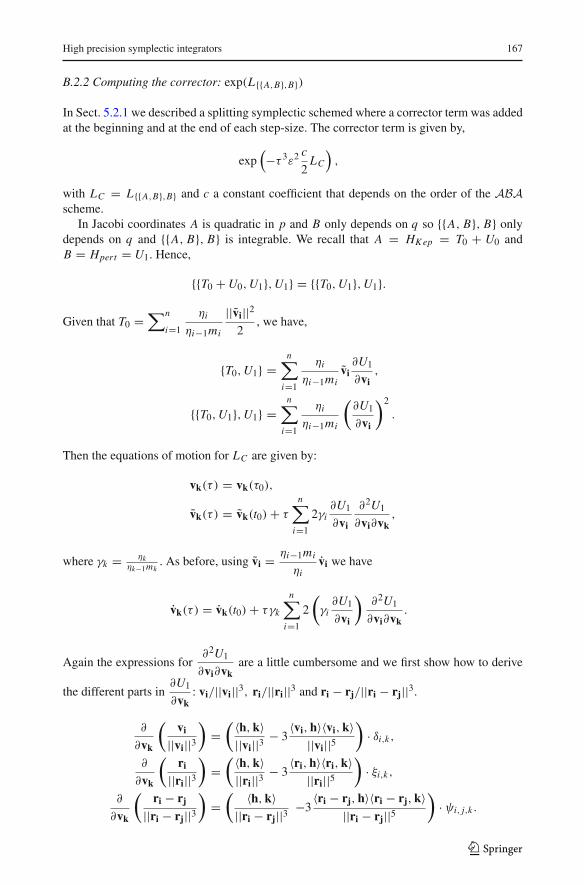
B.2.2 Computing the corrector: exp(L{{A,B},B})
In Sect. 5.2.1 we described a splitting symplectic schemed where a corrector term was addedat the beginning and at the end of each step-size. The corrector term is given by,
exp(−τ 3ε2 c
2LC
),
with LC = L{{A,B},B} and c a constant coefficient that depends on the order of the ABAscheme.
In Jacobi coordinates A is quadratic in p and B only depends on q so {{A, B}, B} onlydepends on q and {{A, B}, B} is integrable. We recall that A = HK ep = T0 + U0 andB = Hpert = U1. Hence,
{{T0 + U0,U1},U1} = {{T0,U1},U1}.
Given that T0 =∑n
i=1
ηi
ηi−1mi
||vi||22
, we have,
{T0,U1} =n∑
i=1
ηi
ηi−1mivi∂U1
∂vi,
{{T0,U1},U1} =n∑
i=1
ηi
ηi−1mi
(∂U1
∂vi
)2
.
Then the equations of motion for LC are given by:
vk(τ ) = vk(τ0),
vk(τ ) = vk(t0)+ τ
n∑
i=1
2γi∂U1
∂vi
∂2U1
∂vi∂vk,
where γk = ηkηk−1mk
. As before, using vi = ηi−1mi
ηivi we have
vk(τ ) = vk(t0)+ τγk
n∑
i=1
2
(
γi∂U1
∂vi
)∂2U1
∂vi∂vk.
Again the expressions for∂2U1
∂vi∂vkare a little cumbersome and we first show how to derive
the different parts in∂U1
∂vk: vi/||vi||3, ri/||ri||3 and ri − rj/||ri − rj||3.
∂
∂vk
(vi
||vi||3)
=( 〈h,k〉
||vi||3 − 3〈vi,h〉〈vi,k〉
||vi||5)
· δi,k,
∂
∂vk
(ri
||ri||3)
=( 〈h,k〉
||ri||3 − 3〈ri,h〉〈ri,k〉
||ri||5)
· ξi,k,
∂
∂vk
(ri − rj
||ri − rj||3)
=( 〈h,k〉
||ri − rj||3 −3〈ri − rj,h〉〈ri − rj,k〉
||ri − rj||5)
· ψi, j,k .
123
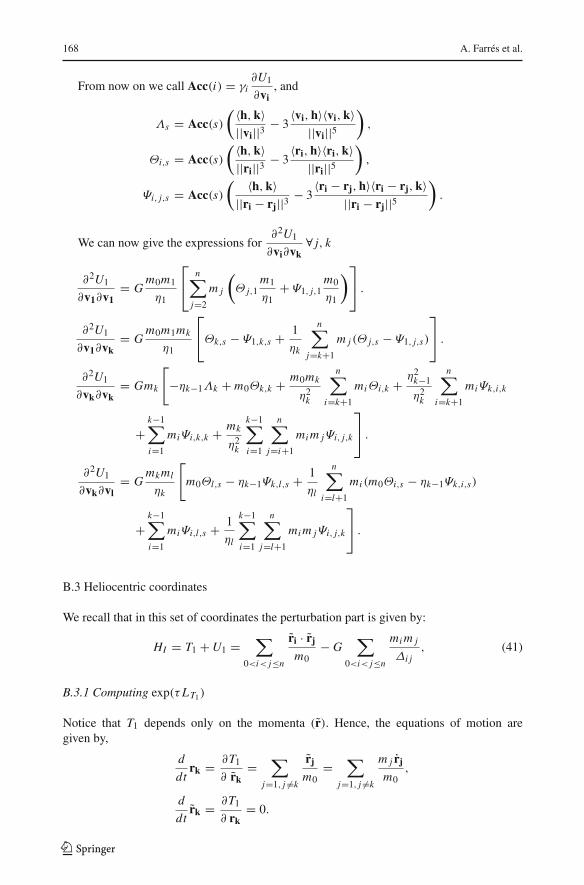
168 A. Farrés et al.
From now on we call Acc(i) = γi∂U1
∂vi, and
Λs = Acc(s)( 〈h,k〉
||vi||3 − 3〈vi,h〉〈vi,k〉
||vi||5)
,
Θi,s = Acc(s)( 〈h,k〉
||ri||3 − 3〈ri,h〉〈ri,k〉
||ri||5)
,
Ψi, j,s = Acc(s)( 〈h,k〉
||ri − rj||3 − 3〈ri − rj,h〉〈ri − rj,k〉
||ri − rj||5)
.
We can now give the expressions for∂2U1
∂vi∂vk∀ j, k
∂2U1
∂v1∂v1= G
m0m1
η1
⎡
⎣n∑
j=2
m j
(
Θ j,1m1
η1+ Ψ1, j,1
m0
η1
)⎤
⎦ .
∂2U1
∂v1∂vk= G
m0m1mk
η1
⎡
⎣Θk,s − Ψ1,k,s + 1
ηk
n∑
j=k+1
m j (Θ j,s − Ψ1, j,s)
⎤
⎦ .
∂2U1
∂vk∂vk= Gmk
[
−ηk−1Λk + m0Θk,k + m0mk
η2k
n∑
i=k+1
miΘi,k + η2k−1
η2k
n∑
i=k+1
miΨk,i,k
+k−1∑
i=1
miΨi,k,k + mk
η2k
k−1∑
i=1
n∑
j=i+1
mi m jΨi, j,k
⎤
⎦ .
∂2U1
∂vk∂vl= G
mkml
ηk
[
m0Θl,s − ηk−1Ψk,l,s + 1
ηl
n∑
i=l+1
mi (m0Θi,s − ηk−1Ψk,i,s)
+k−1∑
i=1
miΨi,l,s + 1
ηl
k−1∑
i=1
n∑
j=l+1
mi m jΨi, j,k
⎤
⎦ .
B.3 Heliocentric coordinates
We recall that in this set of coordinates the perturbation part is given by:
HI = T1 + U1 =∑
0<i< j≤n
ri · rj
m0− G
∑
0<i< j≤n
mi m j
Δi j, (41)
B.3.1 Computing exp(τ LT1)
Notice that T1 depends only on the momenta (r). Hence, the equations of motion aregiven by,
d
dtrk = ∂T1
∂ rk=
∑
j=1, j �=k
rj
m0=
∑
j=1, j �=k
m j rj
m0,
d
dtrk = ∂T1
∂ rk= 0.
123

High precision symplectic integrators 169
Finally,
rk(τ ) = rk(τ0)+ τ∑
j=1, j �=k
m j rj
m0, rk(τ ) = rk(τ0).
B.3.2 Computing exp(τ LU1)
Notice that U1 depends only on the positions (r). Hence, the equations of motion are givenby,
d
dtrk = ∂U1
∂ rk= 0,
d
dtrk = −∂U1
∂ rk= −G
⎛
⎝k−1∑
j=1
mkm j
Δ3k j
(rk − rj)−n∑
j=k+1
mkm j
Δ3jk
(rj − rk)
⎞
⎠ .
Given that rk = mk rk, we have:
rk(τ ) = rk(τ0), rk(τ ) = rk(τ0)− τ G
⎛
⎝k−1∑
j=1
m j
Δ3k j
(rk − rj)+n∑
j=k+1
m j
Δ3k j
(rk − rj)
⎞
⎠ .
Appendix C: Heliocentric coordinates (alternatives for the set of equations)
The canonical heliocentric (CH) coordinates used in Sect. 6 are canonical and the position ofeach body is taken with respect to the position of the Sun. The position and their associatedmomenta are given by:
r0 = u0ri = ui − u0
}
,r0 = u0 + · · · + unri = ui
}
.
The main difference between Jacobi and heliocentric coordinates is that in the second set ofcoordinates the kinetic energy is not diagonal in the momenta. Instead we have:
T = 1
2
n∑
i=0
||ui||2mi
= 1
2
n∑
i=1
||ri||2mi
+ 1
2
|| ∑ni=1 ri||2m0
, (42)
which can be rewritten as:
T = 1
2
n∑
i=0
||ui||2mi
= 1
2
n∑
i=1
||ri||2[
1
m0+ 1
mi
]
+∑
0<i< j
ri · rj
m0. (43)
The extra term due to the momenta of the Sun is added to the perturbation part andmakes it depend on both position and velocities. In Sect. 3 we used Eq. 43 to derive theHamiltonian expression, as in Laskar (1990b, 1991), Koseleff (1993a). Duncan et al. (1998)used Eq. 42 instead, and a Keplerian approximation in which the planets orbits around afixed Sun (Eq. 48). Following Laskar (1991) we will call the first set of equations CH, andfollowing Duncan et al. (1998) we will call the second set of equations democratic canonicalheliocentric (DCH). Here we discuss the main differences between the two sets of equationsand compare the performance of the integrators presented in this paper for both expressions.
123

170 A. Farrés et al.
C.1 Two different expressions for Heliocentric coordinates
As we know in heliocentric coordinates the Hamiltonian for an n-planetary system takes theform:
H = HK + T1 + U1,
a sum of Keplerian parts, a quadratic term in the momenta and the gravitational interactionbetween the other planets. Using Eq. 43 we have, for CH decomposition
HK =n∑
i=1
(1
2||ri||2
[m0 + mi
m0mi
]
− Gm0mi
||ri||)
, (44)
T1 =∑
0<i< j≤n
ri · rj
m0, (45)
U1 = −G∑
0<i< j≤n
mi m j
Δi j. (46)
The main advantage of this way to split the equations is that Kepler’s third law is satisfiedfor the individual planets: n2a3 = G(m0 + mi ). But HI = T1 + U1 is not integrable and{T1,U1} �= 0.
Using Eq. 42 we have the DCH splitting introduced by Duncan et al. (1998), and usedlater on by Chambers (1999) and Wisdom (2006)
H∗K =
n∑
i=1
(1
2
||ri||2mi
− Gm0mi
||ri||)
, (47)
T ∗1 = 1
2
|| ∑ni=1 ri||2m0
, (48)
U∗1 = −G
∑
0<i< j≤n
mi m j
Δi j. (49)
With this way to split the equations the mass parameter for the Keplerian orbits is μ = Gm0
for all of the planets. On the other hand, T ∗1 and U∗
1 (Eqs. 48–49) commute, i.e. {T ∗1 ,U
∗1 } =
0 and this is a advantage when we build high order splitting schemes. For simplicity letus consider HB = T1 and HC = U1 for both expressions. We recall that in heliocentriccoordinates we need to integrate exp(τ (B +C)). Using DCH splitting (Eqs. 48–49) we have:
exp(τ (B + C)) = exp(τ B) exp(τC), (50)
which can be computed exactly and does not introduce any extra error terms to the splittingschemes discussed in Sect. 5. Instead, using CH variables (Eqs. 45–46) we used
exp(τ (B + C)) ≈ exp(τ
2C
)exp(τ B) exp
(τ
2C
), (51)
and introduced error terms of order ε3τ 2. To deal with this in Sect. 6 derived splitting schemeswhere an extra stage was added to get rid of these extra error terms.
123

High precision symplectic integrators 171
-18
-16
-14
-12
-10
-8
-6
-5 -4 -3 -2 -1
Mer - Ven - Ear - Mar
ABA82 CHABAH844 CH
ABAH1064 CHABA82 DCHABA84 DCH
ABA1064 DCH
-18
-16
-14
-12
-10
-8
-6
-5 -4 -3 -2 -1
Jup - Sat - Ura - Nep
ABA82 CHABAH844 CH
ABAH1064 CHABA82 DCHABA84 DCH
ABA1064 DCH
-18
-16
-14
-12
-10
-8
-6
-5 -4 -3 -2 -1
Mercury to Neptune
ABA82 CHABAH844 CH
ABAH1064 CHABA82 DCHABA84 DCH
ABA1064 DCH
(Helio vs Helio) (Helio vs Helio)(Helio vs Helio)
Fig. 9 Comparison between the two expressions for heliocentric coordinates: the classical CH expressions(Eqs. 44–46) continuous lines and the DCH expressions (Eqs. 47–49) discontinuous lines. For the schemesABA82 (red), ABA84 (green) and ABA1064 (blue). From left to right the 4 inner planets, the 4 outer planetsand the whole Solar System. The x-axis represents the cost (τ/s) of the method and the y-axis the maximumenergy variation for one integration with constant step-size τ (decimal log scales)
C.2 Comparisons between the expressions
We recall that when we use DCH variables (Eqs. 47–49) we use the splitting schemes dis-cussed in Sect. 5 with
S(τ ) =n∏
i=1
exp(aiτ L HK∗ ) exp(biτ LT ∗1) exp(biτ LU∗
1). (52)
While when we use the classical CH variables (Eqs. 44–46) we use the splitting schemesdiscussed in Sect. 6 with
S(τ ) =n∏
i=1
exp(aiτ L HK ep ) exp(
biτ
2LT1
)exp(biτ LU1) exp
(biτ
2LT1
). (53)
We compare the ABA schemes of orders (8, 2), (8, 4) and (10, 6, 4) for both splittingexpressions. We recall that the schemes of order (8, 4) and (10, 6, 4) that use CH variables(Eqs. 44–46) have one more stage than the schemes used with DCH variables (Eqs. 47–49).
Figure 9 summarise the performance of the different integrating schemes presented inSects. 5 and 6. From left to right we have the results for the inner planets, the outer planetsand the whole Solar System. The red lines show the performance of the ABA82 scheme, thegreen lines are for the ABA84 schemes and the blue lines are for the ABA1064 schemes.We use continuous lines when we consider CH variables and discontinuous lines for DCHvariables.
As we can see, there is no significant difference between using one splitting or the other. Insome cases one is better that the other. The main advantage that the splitting DCH introducedby Duncan et al. (1998) is that we do not require an extra stage for a high-order scheme.
123

172 A. Farrés et al.
-30
-25
-20
-15
-10
-5
-6 -5 -4 -3 -2 -1 0
ABA82ABA84
ABA104ABA864
ABA1064
-30
-25
-20
-15
-10
-5
-6 -5 -4 -3 -2 -1 0
ABA82ABA84
ABA104ABA864
ABA1064
-30
-25
-20
-15
-10
-5
-6 -5 -4 -3 -2 -1 0
ABA82ABA84
ABA104ABA864
ABA1064
Mer - Ven - Ear - Mar (Jacobi Coord)
Jup - Sat - Ura - Nep (Jacobi Coord)
Mercury to Neptune (Jacobi Coord)
Fig. 10 Comparison using Jacobi coordinates between the ABA82, ABA84, ABA104, ABA864 andABA1064 schemes using quadruple precision arithmetics. From left to right the 4 inner planets, the 4 outerplanets and the whole Solar System. The x-axis represents the cost (τ/s) and the y-axis the maximum energyvariation for one integration with constant step-size τ (decimal log scales)
-30
-25
-20
-15
-10
-5
-6 -5 -4 -3 -2 -1 0
ABAH82ABAH844ABAH864
ABAH1064
-30
-25
-20
-15
-10
-5
-6 -5 -4 -3 -2 -1 0
ABAH82ABAH844ABAH864
ABAH1064
-30
-25
-20
-15
-10
-5
-6 -5 -4 -3 -2 -1 0
ABAH82ABAH844ABAH864
ABAH1064
Mer - Ven - Ear - Mar (Helio Coord)
Jup - Sat - Ura - Nep (Helio Coord)
Mercury to Neptune
(Helio Coord)
Fig. 11 Comparison using heliocentric coordinates between the ABAH82, ABAH84, ABAH864 andABAH1064 schemes using quadruple precision arithmetics. From left to right the 4 inner planets, the 4outer planets and the whole Solar System. The x-axis represents the cost (τ/s) and the y-axis the maximumenergy variation for one integration with constant step-size τ (decimal log scales)
Appendix D: Comparison in quadruple precision
As we have discussed throughout the article, in many cases we have seen that despite takinghigher order methods no significant improvement on the performance of the schemes wasobserved. This is the case of the 4 inner planets in the Solar System, where the size of theperturbation is so small that the extra stages to increase the order of the schemes are useless.Here the round-off error dominates the terms in ε2 and ε4. Similar results are also observedwhen we consider the whole Solar System. In order to see an improvement we need to usehigher precision arithmetics. Here we have repeated the test from Sects. 5 and 6 for the
123
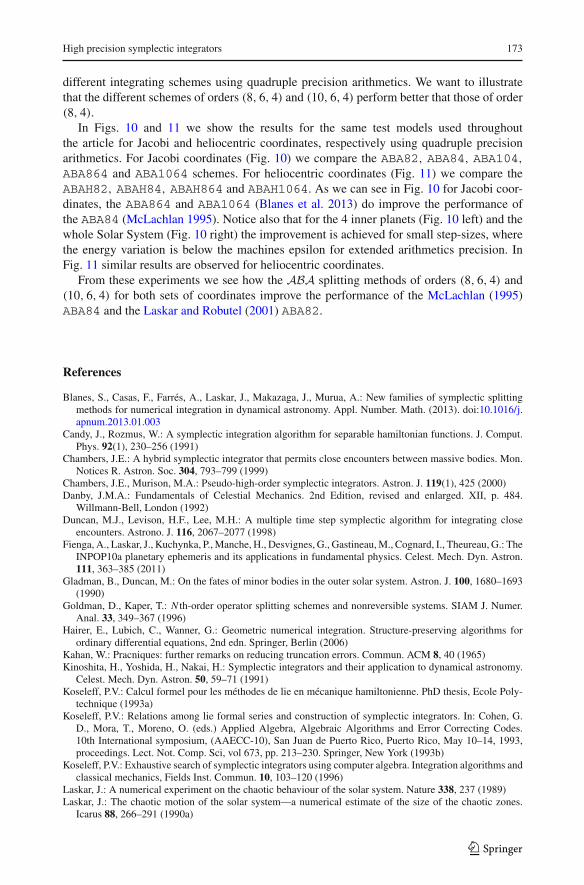
High precision symplectic integrators 173
different integrating schemes using quadruple precision arithmetics. We want to illustratethat the different schemes of orders (8, 6, 4) and (10, 6, 4) perform better that those of order(8, 4).
In Figs. 10 and 11 we show the results for the same test models used throughoutthe article for Jacobi and heliocentric coordinates, respectively using quadruple precisionarithmetics. For Jacobi coordinates (Fig. 10) we compare the ABA82, ABA84, ABA104,ABA864 and ABA1064 schemes. For heliocentric coordinates (Fig. 11) we compare theABAH82, ABAH84, ABAH864 and ABAH1064. As we can see in Fig. 10 for Jacobi coor-dinates, the ABA864 and ABA1064 (Blanes et al. 2013) do improve the performance ofthe ABA84 (McLachlan 1995). Notice also that for the 4 inner planets (Fig. 10 left) and thewhole Solar System (Fig. 10 right) the improvement is achieved for small step-sizes, wherethe energy variation is below the machines epsilon for extended arithmetics precision. InFig. 11 similar results are observed for heliocentric coordinates.
From these experiments we see how the ABA splitting methods of orders (8, 6, 4) and(10, 6, 4) for both sets of coordinates improve the performance of the McLachlan (1995)ABA84 and the Laskar and Robutel (2001) ABA82.
References
Blanes, S., Casas, F., Farrés, A., Laskar, J., Makazaga, J., Murua, A.: New families of symplectic splittingmethods for numerical integration in dynamical astronomy. Appl. Number. Math. (2013). doi:10.1016/j.apnum.2013.01.003
Candy, J., Rozmus, W.: A symplectic integration algorithm for separable hamiltonian functions. J. Comput.Phys. 92(1), 230–256 (1991)
Chambers, J.E.: A hybrid symplectic integrator that permits close encounters between massive bodies. Mon.Notices R. Astron. Soc. 304, 793–799 (1999)
Chambers, J.E., Murison, M.A.: Pseudo-high-order symplectic integrators. Astron. J. 119(1), 425 (2000)Danby, J.M.A.: Fundamentals of Celestial Mechanics. 2nd Edition, revised and enlarged. XII, p. 484.
Willmann-Bell, London (1992)Duncan, M.J., Levison, H.F., Lee, M.H.: A multiple time step symplectic algorithm for integrating close
encounters. Astrono. J. 116, 2067–2077 (1998)Fienga, A., Laskar, J., Kuchynka, P., Manche, H., Desvignes, G., Gastineau, M., Cognard, I., Theureau, G.: The
INPOP10a planetary ephemeris and its applications in fundamental physics. Celest. Mech. Dyn. Astron.111, 363–385 (2011)
Gladman, B., Duncan, M.: On the fates of minor bodies in the outer solar system. Astron. J. 100, 1680–1693(1990)
Goldman, D., Kaper, T.: N th-order operator splitting schemes and nonreversible systems. SIAM J. Numer.Anal. 33, 349–367 (1996)
Hairer, E., Lubich, C., Wanner, G.: Geometric numerical integration. Structure-preserving algorithms forordinary differential equations, 2nd edn. Springer, Berlin (2006)
Kahan, W.: Pracniques: further remarks on reducing truncation errors. Commun. ACM 8, 40 (1965)Kinoshita, H., Yoshida, H., Nakai, H.: Symplectic integrators and their application to dynamical astronomy.
Celest. Mech. Dyn. Astron. 50, 59–71 (1991)Koseleff, P.V.: Calcul formel pour les méthodes de lie en mécanique hamiltonienne. PhD thesis, Ecole Poly-
technique (1993a)Koseleff, P.V.: Relations among lie formal series and construction of symplectic integrators. In: Cohen, G.
D., Mora, T., Moreno, O. (eds.) Applied Algebra, Algebraic Algorithms and Error Correcting Codes.10th International symposium, (AAECC-10), San Juan de Puerto Rico, Puerto Rico, May 10–14, 1993,proceedings. Lect. Not. Comp. Sci, vol 673, pp. 213–230. Springer, New York (1993b)
Koseleff, P.V.: Exhaustive search of symplectic integrators using computer algebra. Integration algorithms andclassical mechanics, Fields Inst. Commun. 10, 103–120 (1996)
Laskar, J.: A numerical experiment on the chaotic behaviour of the solar system. Nature 338, 237 (1989)Laskar, J.: The chaotic motion of the solar system—a numerical estimate of the size of the chaotic zones.
Icarus 88, 266–291 (1990a)
123

174 A. Farrés et al.
Laskar, J.: Les Méthodes Modernes de la Mecánique Céleste (Goutelas, France, 1989), Editions Frontières,chap Systèmes de Variables et Eléments, pp. 63–87 (1990b)
Laskar, J.: Analytical framework in poincaré variables for the motion of the solar system. In: Roy, A. (ed.)Predictability, Stability, and Chaos in N-Body Dynamical Systems, pp. 93–114. NATO, Plenum Press, ASI(1991)
Laskar, J., Robutel, P.: High order symplectic integrators for perturbed hamiltonian systems. Celest. Mech.Dyn. Astron. 80, 39–62 (2001)
Laskar, J., Quinn, T., Tremaine, S.: Confirmation of resonant structure in the solar system. Icarus 95, 148–152(1992)
Laskar, J., Robutel, P., Joutel, F., Gastineau, M., Correia, A.C.M., Levrard, B.: A long-term numerical solutionfor the insolation quantities of the earth. Astron. Astrophys. 428, 261–285 (2004)
Laskar, J., Fienga, A., Gastineau, M., Manche, H.: La2010: a new orbital solution for the long-term motionof the earth. Astron. Astrophys. 532, 89 (2011a)
Laskar, J., Gastineau, M., Delisle, J.B., Farrés, A., Fienga, A.: Strong chaos induced by close encounters withceres and vesta. Astron. Astrophys. 532, L4 (2011b)
Lourens, L. J., Hilgen, F. J., Shackleton, N. J., Laskar, J., Wilson, D.: The neogene period. In: Gradstein, F.,Ogg, J., Smith, A. (eds.) A Geologic. Time scale, pp 409–440. Cambridge University Press, UK (2004)
McLachlan, R.I.: Composition methods in the presence of small parameters. BIT Numer. Math. 35, 258–268(1995)
McLachlan, R.I.: Families of high-order composition methods. Numer. Algorithms 31, 233–246 (2002)McLachlan, R., Quispel, R.: Splitting methods. Acta Numerica 11, 341–434 (2002)Milankovitch, M.: Kanon der Erdbestrahlung und seine Anwendung auf das Eiszeitenproblem. Spec. Acad.
R, Serbe, Belgrade (1941)Morbidelli, A.: Modern integrations of solar system dynamics. Annu. Rev. Earth Planet. Sci. 30, 89–112
(2002)Murua, A., Sanz-Serna, J.: Order conditions for numerical integrators obtained by composing simpler inte-
grators. Philos. Trans. R. Soc. Lond. Ser. A Math. Phys. Eng. Sci. 357(1754), 1079–1100 (1999)Quinn, T.R., Tremaine, S., Duncan, M.: A three million year integration of the earth’s orbit. Astron. J. 101,
2287–2305 (1991)Saha, P., Tremaine, S.: Long-term planetary integration with individual time steps. Astron. J. 108, 1962–1969
(1994)Sheng, Q.: Solving linear partial differential equations by exponential splitting. IMA J. Numer. Anal. 9,
199–212 (1989)Sussman, G.J., Wisdom, J.: Chaotic evolution of the solar system. Science 257, 56–62 (1992)Suzuki, M.: Fractal decomposition of exponential operators with applications to many-body theories and
monte carlo simulations. Phys. Lett. A 146(6), 319–323 (1990)Suzuki, M.: General theory of fractal path integrals with applications to many-body theories and statistical
physics. J. Math. Phys. 32(2), 400–407 (1991)Touma, J., Wisdom, J.: Lie-poisson integrators for rigid body dynamics in the solar system. Astron. J. 107,
1189–1202 (1994)Viswanath, D.: How many timesteps for a cycle? Analysis of the Wisdom–Holman algorithm. BIT Numer.
Math. 42, 194–205 (2002)Wisdom, J.: Symplectic correctors for canonical heliocentric n-body maps. Astron. J. 131(4), 2294 (2006)Wisdom, J., Holman, M.: Symplectic maps for the n-body problem. Astron. J. 102, 1528–1538 (1991)Wisdom, J., Holman, M., Touma, J.: Symplectic correctors. Fields Inst. Commun. 10, 217 (1996)Yoshida, H.: Construction of higher order symplectic integrators. Phys. Lett. A 150(5–7), 262–268 (1990)
123


![Symplectic propagators for the Kepler problem with time ...personales.upv.es/serblaza/2018_Kepler_t_dep.pdf · 2 Philipp Bader et al. of an integrable system [4], but in addition](https://img.pdfslide.us/doc/110x75/5dd0ece6d6be591ccb635e31/symplectic-propagators-for-the-kepler-problem-with-time-2-philipp-bader-et-al.jpg)