J. Acoustic Emission, 23 (2005) 81 © 2005 Acoustic Emission Group

HIGH PRECISION GEOPHONE CALIBRATION

MASAHIRO KAMATA

Schlumberger K.K., 2-2-1 Fuchinobe, Sagamihara, Kanagawa 229-0006 Japan

Abstract

Geophones are commonly used in seismic signal detection and are widely sold with response

parameters with specified tolerances. High precision seismic analysis can extract subtle infor-

mation from seismic records, but requires knowledge of the in-situ response parameters of the

sensors. The geophone response is specified at room temperature; however, geophone response

changes with the orientation with respect to gravity, temperature and aging. The changes due to

temperature and tilt may exceed the tolerance limits, so there is a need to perform in-situ calibra-

tion to know the exact response. In the impedance calibration method, the impedance of a geo-

phone can be measured by injecting current. From the impedance, it is possible to describe all of

the response parameters except for the moving mass. The dynamic method is also known for

calibration of a vibration sensor relative to a reference sensor. The reference sensor can be fabri-

cated with a pre-measured moving-coil mass so that all the geophone parameters can be deter-

mined. Alternatively the reference sensor can be calibrated by using a reciprocity method mak-

ing use of three vibration sensors. We have developed unique geophones that output signals

proportional to acceleration. Complete calibration schemes have been established, and all the

geophones are fully calibrated during the manufacturing process. A method has been described

to re-evaluate the geophone’s moving mass to make in-situ calibration in the working environ-

ment with the impedance method.

Keywords: Geophone, Seismic sensors, Moving-coil accelerometer, Calibration, Impedancemethod

1. Introduction

A geophone consists of a pair of moving coils suspended in a magnetic field by means of a

pair of springs as shown in Fig. 1. The spring is usually pre-stressed to compensate the natural

displacement of the coil due to gravitational force so that the coil is centered in the magnetic

field.

The output of a geophone is usually terminated by a shunt resistance R as shown in Fig. 2 to

provide external damping. The current flowing in the moving coil reduces coil motion. The

amount of shunt resistance is chosen so that the total damping factor is 70%.

The equation of motion for the moving coil relative to the magnetic flux for given external

displacement u may be written as;

Blidt

udmk

dt

dc

dt

dm =++

2

2

2

2

(1)

where : coil displacement; k: spring constant; m: moving mass of coil; c: friction coefficient; g:

gravitational acceleration; B: magnetic flux density; l: length of coil wire; i: current; u: external

displacement.

82

Fig. 1 Structure of a geophone.

Fig. 2 Damping control.

is the relative position of the moving coil inside the geophone. The first term in the left

hand side of equation (1) is the inertial force, the second term is the friction force proportional to

the velocity, and the last term is the spring force. The summation of the three forces balances

with the force due to external displacement and the damping force caused by the electric current.

The electric signal generated by the moving coil is expressed in terms of magnetic flux den-

sity, length of coil wire and velocity of the coil as;

dt

dBleg = (2)

For a given external displacement, )sin( tau = , the response may be expressed as;

)sin(= tAeg (3)

The amplitude response and phase may be found from equations (1), (2) and (3) as;

2

0

22

0

2

0

0

21 +

=

S

aA and ( )2

0

0

1

2

tan = (4, 5)

where

m

k=

0,

( )0

2

0

0

2 mRr

S

++= ,

0

0

2m

c= , and BlS =

0.

The geophone parameters are the natural frequency f0, the open circuit sensitivity S0, the open

circuit damping, the coil resistance r, and the moving mass m. The response of a geophone is

determined with four geophone parameters and the shunt resistance R.

For > 0, equation (3) may be approximated as )cos()(0 taSeg = . The sensitivity is

proportional to the velocity (a ) of the vibration at above the natural frequency. Figure 3 shows

83

Fig. 3 Geophone response.

the amplitude response eg/S0(a ) and phase response of a geophone with 10 Hz natural fre-

quency and 0.7 damping.

2. Geophone Response in Measurement Environment

Coil resistance is almost double at 200˚C and open circuit damping is reduced by 20% as

shown in Figs. 4 and 5. Natural frequency f0, and the open circuit sensitivity S0 change by a few

percent each. (Figs. 6 and 7)

The geophone parameters are measured when the geophone is positioned vertically. In prac-

tice, geophones are planted by stamping into the ground by foot, and so are not necessarily verti-

cal. In borehole seismic acquisition, a downhole tool with geophones is deployed in a borehole

that may not be vertical. Figures 8, 9 and 10 show measured results of a geophone under tilt.

There is a few percentage points change observed at ±30˚ tilt.

Fig. 4 Coil resistance change. Fig. 5 Natural frequency change.

84

Fig. 6 Open circuit damping change. Fig. 7 Sensitivity change.

Fig. 8 Natural frequency shift by tilt. Fig. 9 Open circuit damping shift by tilt.

Fig. 10 Open circuit sensitivity shift by tilt.

3. Geophone Accelerometer

We have developed a unique geophone that responds to acceleration between 1/10 x f0 and

10 x f0. A light moving coil is suspended in a strong magnetic flux density.

The imaginary short circuit of an operational amplifier applies a large damping current so

that the geophone responds to acceleration at near its natural frequency. See the schematic dia-

gram in Fig. 11. For = 0, equation (3) may be approximated as

)sin(2)(

0

02t

Saeg = . (6)

Equation (6) shows that a response is in proportion to acceleration. In general, equation (3)

is rewritten as acceleration form (7);

85

Fig. 11 Imagenary short circuit.

Fig. 12 GAC response.

)sin(

21

)(2

0

22

0

00

0

2

+

= t

S

aeg . (7)

When the damping factor is large, the damping term in equation (7) becomes dominant and

the frequency range becomes wider. The natural frequency is chosen to be in the middle of the

seismic band at about 20 Hz. For this natural frequency, the natural displacement of the coil due

to gravity is not large and the GAC design is omni-tiltable. (See Fig. 12.)

The GAC was originally introduced for borehole seismic acquisition to obsolete the need for

a gimbal-mount mechanism. A second generation GAC sensor is now bring used in seabed and

land seismic recording.

4. Geophone Calibration Method

4.1 Impedance Method

A current runs into the moving coil that is suspended in a magnetic flux B. The force acting

to the moving coil is Bli, where B is the magnetic flux density, l is the effective wire length of the

moving coil and i is the current. The equation of motion for the moving coil may be written as;

Blikdt

dc

dt

dm =++

2

2

(8)

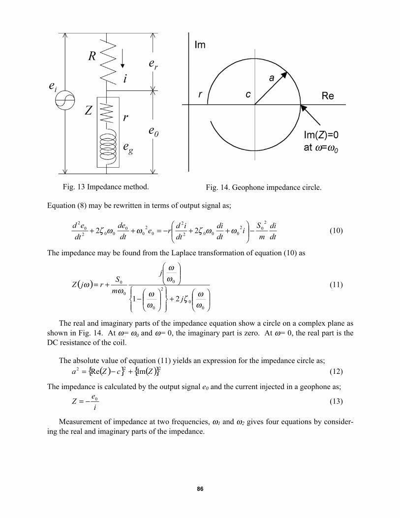
Since the output signal is (see Fig. 13);

rieeg+=

0(9)

86

Fig. 13 Impedance method. Fig. 14. Geophone impedance circle.

Equation (8) may be rewritten in terms of output signal as;

dt

di

m

Si

dt

di

dt

idre

dt

de

dt

ed2

02

0002

2

0

2

0

0

002

0

2

22 ++=++ (10)

The impedance may be found from the Laplace transformation of equation (10) as

( )

+

+=

0

0

2

0

0

0

0

21 j

j

m

SrjZ (11)

The real and imaginary parts of the impedance equation show a circle on a complex plane as

shown in Fig. 14. At = 0 and = 0, the imaginary part is zero. At = 0, the real part is the

DC resistance of the coil.

The absolute value of equation (11) yields an expression for the impedance circle as;

( ){ } ( ){ }222ImRe ZcZa += (12)

The impedance is calculated by the output signal e0 and the current injected in a geophone as;

i

eZ

0= (13)

Measurement of impedance at two frequencies, 1 and 2 gives four equations by consider-

ing the real and imaginary parts of the impedance.

87

( )2

0

1

0

22

0

1

2

0

1

0

0

2

0

1

21

2

Re

+

+=m

S

rZ (14)

( )2

0

1

0

22

0

1

0

1

2

0

1

0

2

0

1

21

1

Im

+

=m

S

Z (15)

( )2

0

2

0

22

0

2

2

0

2

0

0

2

0

2

21

2

Re

+

+=m

S

rZ (16)

( )2

0

2

0

22

0

2

0

2

2

0

2

0

2

0

2

21

1

Im

+

=m

S

Z . (17)

From equations (14-17), it is possible to find the four geophone parameters, r, 0, 0, and S0.

Inserting Z1 and Z2 into Equation (12) gives the center and radius of the impedance circle.

( ) ( ) ( ) ( )

( ) ( ){ }21

2

2

2

1

2

2

2

1

ReRe2

ReReImIm

ZZ

ZZZZc

+= (18)

( ) ( ){ }21

2

1ReIm ZcZa += (19)

The DC resistance r is found to be;

acr = (20)

From impedance equations (14-17), 0, 0, and S0 may be found as,

0=

A1 2

( )1 2

A2 1

( ) where

( )

( )

( )

( )2

1

2

1

Im

Im

Re

Re

Z

Z

rZ

rZA •= (21)

0=

0

2

1

2( ) Re Z1

( ) r{ }2

0 1Im Z

1( ) r{ }

(22)

88

S0=

m Im Z1

( )0

2

1

2( ){ }2

+ 40

2

0

2

1

2

0

2

1

2( ) 1

(23)

4.2 Dynamic Method

In the dynamic calibration method, a geophone is mounted on a shaker with a reference sen-

sor with a known response. The sensitivity may be evaluated as

r

r

g Se

eS 0

= (24)

where

Sg : sensitivity of a geophone to be calibrated

Sr : sensitivity of the reference geophone

e0 : output signal from the geophone to be calibrated

er: output signal from the reference geophone.

Calibrated accelerometers are commonly sold in the market; however, their calibration is

usually to 1% accuracy. It is known that the temperature coefficient of a piezoelectric acceler-

ometer is about 0.1%/˚C; however, the coefficient is not calibrated nor warranted by manufactur-

ers. We do not know if this temperature coefficient can be applied to any calibrated acceler-

ometers we can purchase. A five-degree temperature change can cause 0.5% error, and it is dif-

ficult to measure the temperature of the accelerometer, since the temperature of the housing may

not be the same as the temperature of the piezoelectric element.

Fig. 15 Dynamic method. Fig. 16 Reciprocity calibration.

4.3 Reciprocity Calibration

An alternative to the dynamic method is the reciprocity method of calibration to determine

geophone sensitivities. In the reciprocity method, three geophones are mounted together as

shown in Fig. 16. A current may be injected into a geophone to shake the entire assembly and

the output from the other geophones may be measured. Let eij denote a signal from geophone i

responding to signal input to shaker geophone j. Geophones G2 and G3 output signals are then

e21 and e31 when shaking G1. Then by injecting signal into Geophone G2 we get e32 as the output

89

from G3. A geophone shakes the entire mass M along with three geophones. For the driving

signal te sin0

, the force may be approximated as;

( )t

Z

eSF

j

jsin= (25)

Outputs, e21, e31, and e32 can be expressed in terms of the driving signal. The sensitivity Si of

each geophone may be solved as

( ){ }

( ) ( )iii

i

XZ

Z

e

M

e

eeS

2

2

1

021

1312

1= (26)

( )

( )ii

i

X

Z

e

M

e

eeS

2

013

2312

2= (27)

( )

( )ii

i

X

Z

e

M

e

eeS

2

012

2313

3= (28)

where

Xi( ) =

3

i

2 2( )2

+ 2i i

( )2

(29)

It is then possible to calibrate the sensitivities of three geophones by knowing their impedances.

4.4 Moving Mass Determination and in-situ Calibration

The dynamic method requires a reference geophone for high precision calibration. The

moving coil mass of the reference geophone is measured during assembly. By knowing the

amount of moving mass, the absolute sensitivity can be calibrated by the impedance method.

The reciprocity method can also be used to provide absolute sensitivity calibration. With the ref-

erence geophone, the absolute sensitivity of a geophone may be obtained by the dynamic

method.

In the impedance method, the amount of the moving mass, m was assumed, and the sensitiv-

ity was derived based on the assumed moving mass. If the absolute sensitivity is obtained by the

dynamic or reciprocity method, it is then possible to re-evaluate the moving mass. The absolute

moving mass, m0 may be found by using equations (23) and (24) as2

0

0=

S

Smm

g(30)

The moving mass is a constant that does not change with temperature or tilt of the geophone.

Once the moving mass is known, a geophone can be tested in-situ any time by the impedance

method by injecting current.

5. Conclusion

A high precision geophone calibration method has been established. The method integrates

the impedance and dynamic methods and determines the amount of moving mass. All the Geo-

phone Accelerometers, GACs are fully calibrated during the manufacturing process to determine

DC resistance, natural frequency, open circuit damping, open circuit sensitivity, and moving

mass by impedance and dynamic methods. Since the moving mass does not change with

90

temperature or tilt, it is also possible to make in-situ calibration in the working environment by

just injecting calibration signals. The moving mass does not change in temperature or in tilt. It

is also possible to make in-situ calibration at working environment by just injecting calibration

signals.

References

1) A. Obuchi, M. Kamata: “Moving Coil Accelerometer”, Japanese patent P3098045, H12,

Oct.10

2) A. Obuchi and T. Fujinawa: “Moving Coil Dynamic Accelerometer”, 53rd

EAEG Meeting,

May, 1991 (B021)

3) M. Kamata: “An Accelerometer for Seismic Signal Detection”, Proc. 6th Conference of Un-

derground and Civil Engineering Acoustic Emission, May 1999, Tohoku University, Sendai,

Japan, pp. 25-26.

4) Peter W. Rodgers, Aaron J. Martin, Michelle C. Robertson, Mark M. Hsu, and David B. Har-

ris: "Signal Coil Calibration of E-M seismometers", Bulletin of the Seismological Society of

America, 85, (3), 845-850, June 1995.

5) Mark Harrison, A.O. Sykers, and Paul G. Marcotte: “The Reciprocity Calibration of Piezoe-

lectric Accelerometers”, Journal of Acoustical Society of America, 24, (4), July 1952.

6) Thomas B. Gabrielson: “Apparatus and Method for Calibration of Sensing Transducers”, U.S.patent No. 5,644,067, July 16, 1996.