Embed Size (px)
Citation preview
High Performance Simulation of Internet Worms
David M. NicolDept. of ECE, &
Information Trust InstituteUniversity of Illinois, Urbana-
Champaign
2
problem background
Worm: malware that through automated means gains access to a host, implants a copy of itself, and uses the host to attempt to infect others
Evaluation of defense against worms most readily facilitated by simulation / emulation– e.g. use simulator to generate traffic thrown against
defensesWorms that search for targets can generate a lot of traffic
– fast-scanning worms saturate links and may topple routers
Problems : • Find efficient and accurate ways of simulating infection
growth of random scanning worms• Find efficient and accurate ways of simulating scan traffic
across large networks
3
variance is important
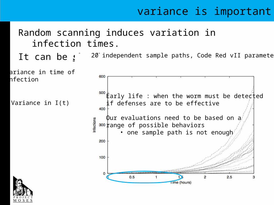
Random scanning induces variation in infection times.
It can be significant20 independent sample paths, Code Red vII parameters
10% of infections
Variance in time of k-thinfection
Variance in I(t)Early life : when the worm must be detectedif defenses are to be effective
Our evaluations need to be based on arange of possible behaviors
• one sample path is not enough
4
detailed model
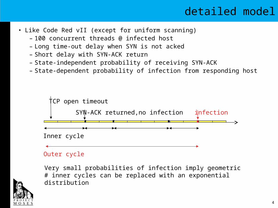
• Like Code Red vII (except for uniform scanning)– 100 concurrent threads @ infected host– Long time-out delay when SYN is not acked– Short delay with SYN-ACK return– State-independent probability of receiving SYN-ACK– State-dependent probability of infection from responding host
TCP open timeout
SYN-ACK returned,no infection infection
Inner cycle
Outer cycle
Very small probabilities of infection imply geometric # inner cycles can be replaced with an exponential distribution
5
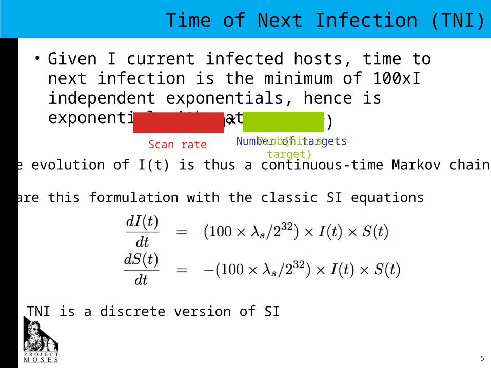
Time of Next Infection (TNI)
• Given I current infected hosts, time to next infection is the minimum of 100xI independent exponentials, hence is exponential with rate
€
(100 × I × λ s) × ((S0 − I) /232)Scan rate Number of targetsProb{hit a target}
State evolution of I(t) is thus a continuous-time Markov chain
Compare this formulation with the classic SI equations
TNI is a discrete version of SI
6
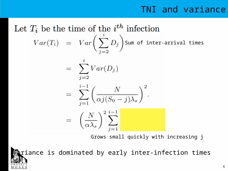
TNI and variance
Sum of inter-arrival times
Grows small quickly with increasing j
Variance is dominated by early inter-infection times
7
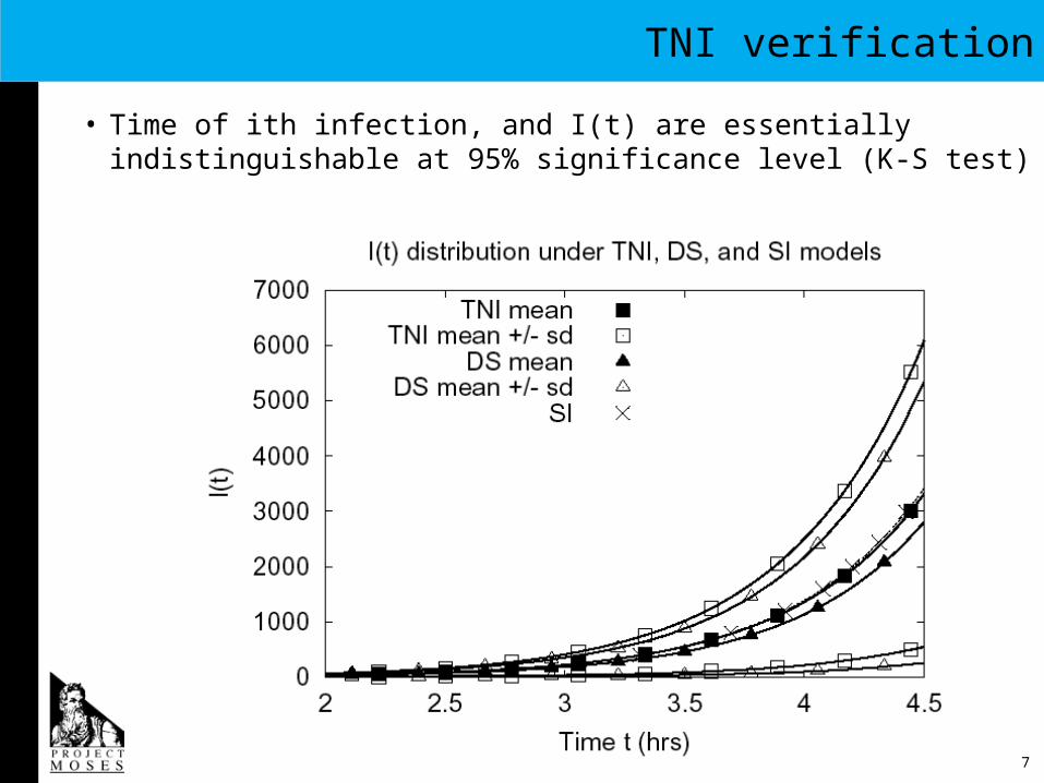
TNI verification
• Time of ith infection, and I(t) are essentially indistinguishable at 95% significance level (K-S test)
8
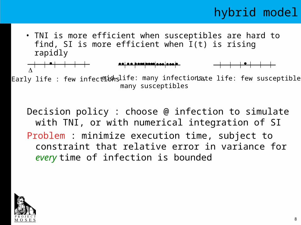
hybrid model
• TNI is more efficient when susceptibles are hard to find, SI is more efficient when I(t) is rising rapidly
Early life : few infections mid-life: many infections,many susceptibles
Late life: few susceptibles
Decision policy : choose @ infection to simulate with TNI, or with numerical integration of SI
Problem : minimize execution time, subject to constraint that relative error in variance for every time of infection is bounded
9
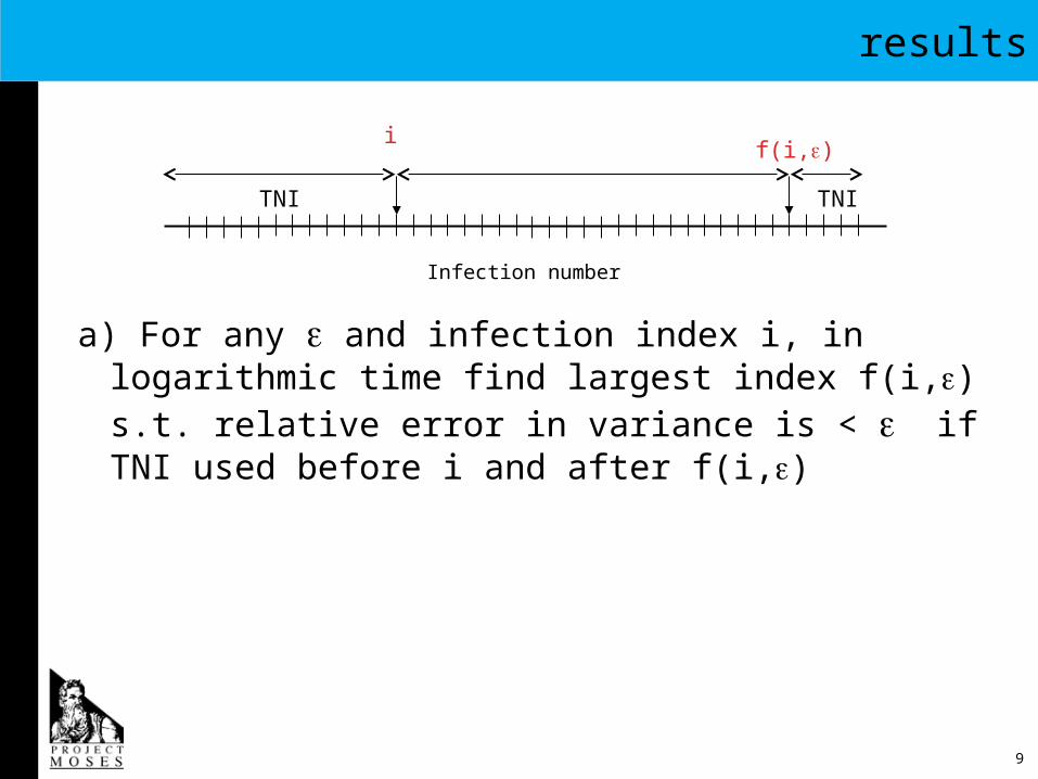
results
a) For any and infection index i, in logarithmic time find largest index f(i,) s.t. relative error in variance is < if TNI used before i and after f(i,)
Infection number
if(i,)
TNI TNI
10
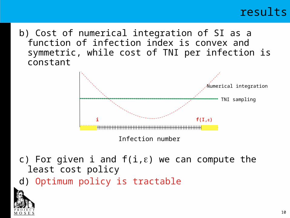
Infection number
Numerical integration
TNI sampling
results
b) Cost of numerical integration of SI as a function of infection index is convex and symmetric, while cost of TNI per infection is constant
c) For given i and f(i,) we can compute the least cost policy
d) Optimum policy is tractable
Numerical integration
i f(I,)
11
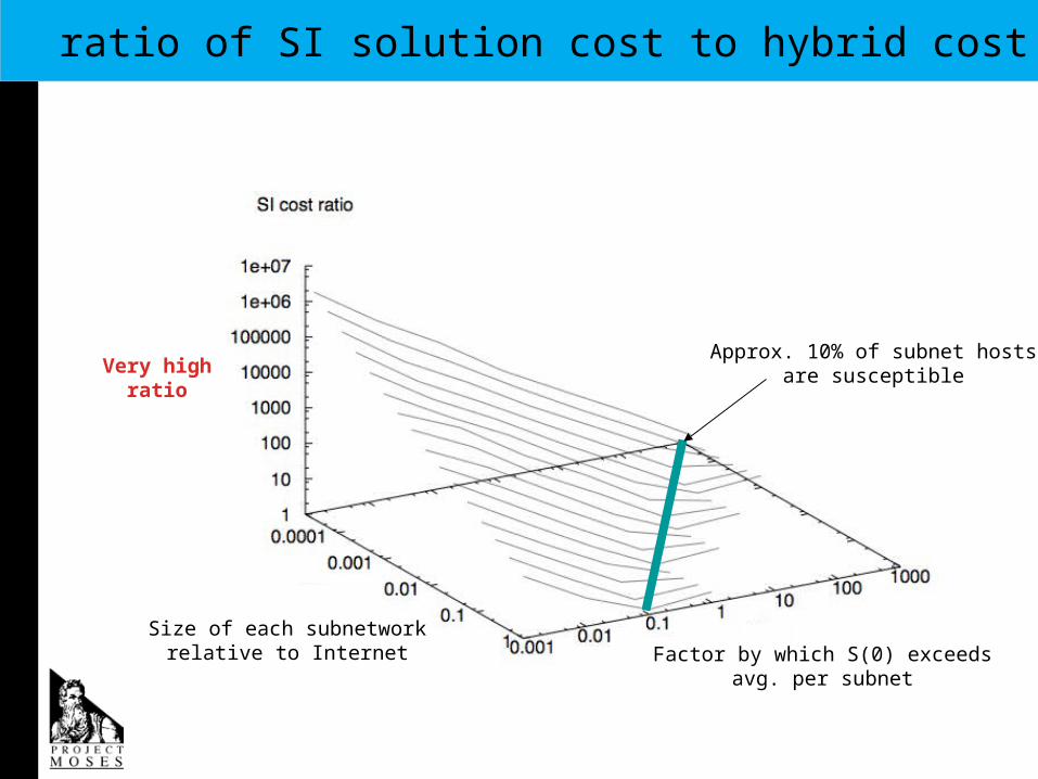
ratio of SI solution cost to hybrid cost
Size of each subnetworkrelative to Internet Factor by which S(0) exceeds
avg. per subnet
Very highratio
Approx. 10% of subnet hostsare susceptible
12
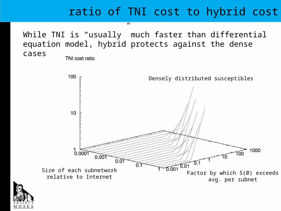
ratio of TNI cost to hybrid cost
Size of each subnetworkrelative to Internet
Factor by which S(0) exceedsavg. per subnet
Densely distributed susceptibles
While TNI is “usually” much faster than differential equation model, hybrid protects against the dense cases
13
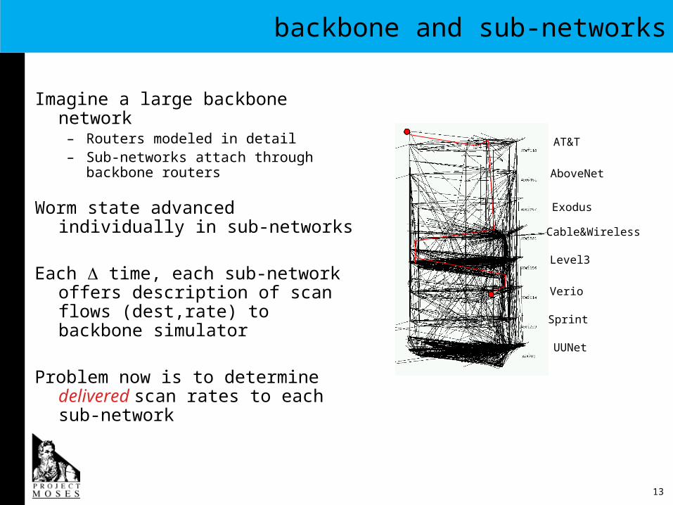
backbone and sub-networks
Imagine a large backbone network– Routers modeled in detail– Sub-networks attach through
backbone routers
Worm state advanced individually in sub-networks
Each time, each sub-network offers description of scan flows (dest,rate) to backbone simulator
Problem now is to determine delivered scan rates to each sub-network
AT&T
AboveNet
Exodus
Cable&Wireless
Level3
Verio
Sprint
UUNet
14
Resolution and Transparency
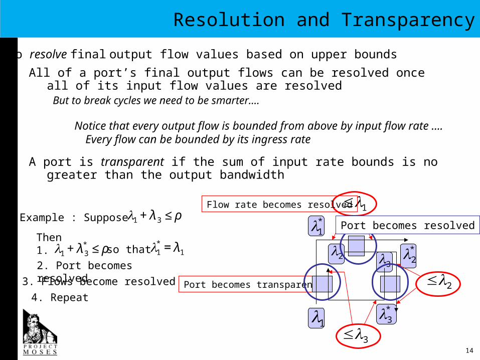
All of a port’s final output flows can be resolved once all of its input flow values are resolvedBut to break cycles we need to be smarter….
A port is transparent if the sum of input rate bounds is no greater than the output bandwidth
€
ρ€
ρ
€
ρ
€
λ1€
λ2
€
λ3
€
λ1*
€
λ3*
€
λ2*
Example : Suppose
€
λ1 + λ 3 ≤ ρ
€
≤λ1
€
≤λ2
€
≤λ3
Then1.
€
λ1 + λ 3* ≤ ρ so that
€
λ1* = λ1
Port becomes transparent
Try to resolve final output flow values based on upper bounds
Notice that every output flow is bounded from above by input flow rate …. Every flow can be bounded by its ingress rate
Flow rate becomes resolved
2. Port becomes resolved
Port becomes resolved
3. Flows become resolved
4. Repeat
15
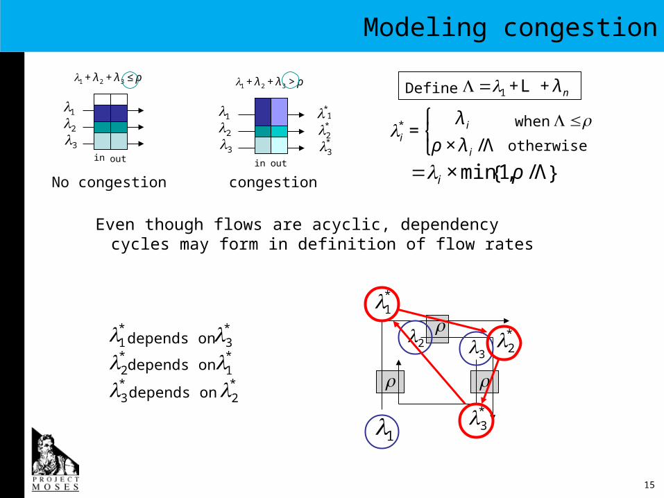
Modeling congestion
Even though flows are acyclic, dependency cycles may form in definition of flow rates
congestion
€
λi* =
λ iρ × λ i /Λ
⎧ ⎨ ⎩
when
€
Λ≤ρotherwise
€
=λi × min 1,ρ /Λ{ }
€
Λ=λ1 +L + λ nDefine
€
λ1
€
λ2
€
λ3
€
λ1 + λ 2 + λ 3 > ρ
in€
λ*1
€
λ2*
€
λ3*
out€
λ1
€
λ2
€
λ3
€
λ1 + λ 2 + λ 3 ≤ ρ
in
€
ρ€
ρ
€
ρ
€
λ1€
λ2
€
λ3
€
λ1*
€
λ3*
€
λ2*
€
λ1*
€
λ3*
depends on
€
λ1*
depends on
€
λ2*
€
λ3*
depends on
€
λ2*
No congestion
out
16
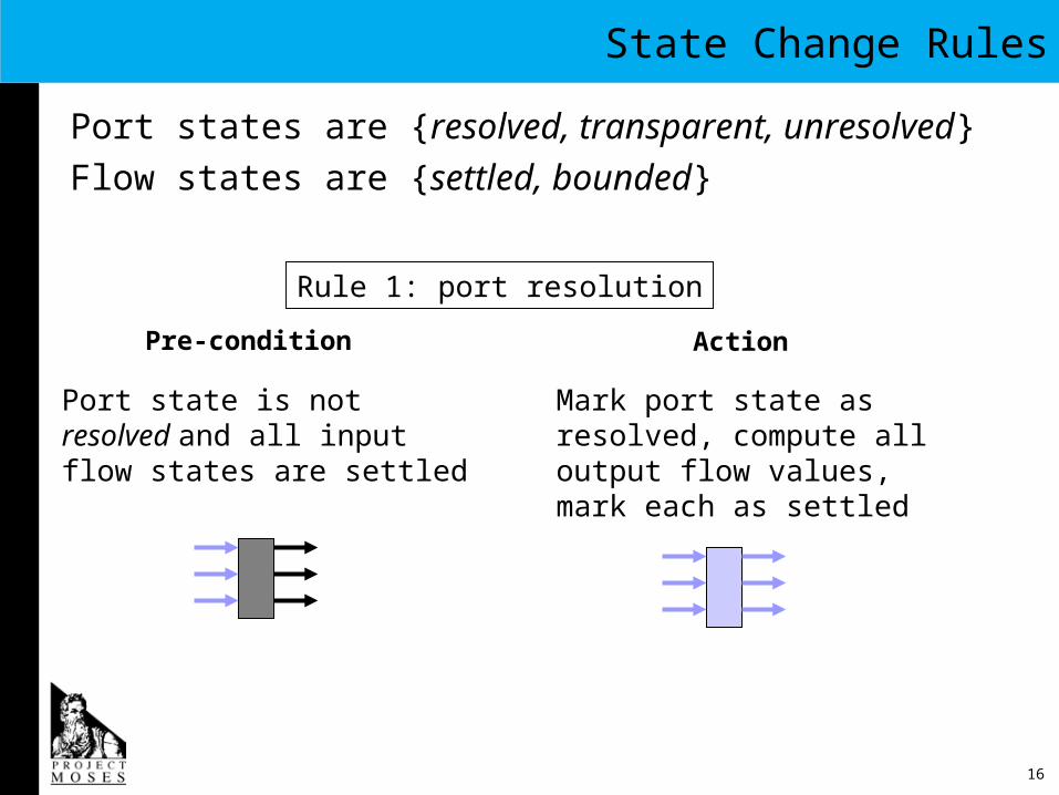
State Change Rules
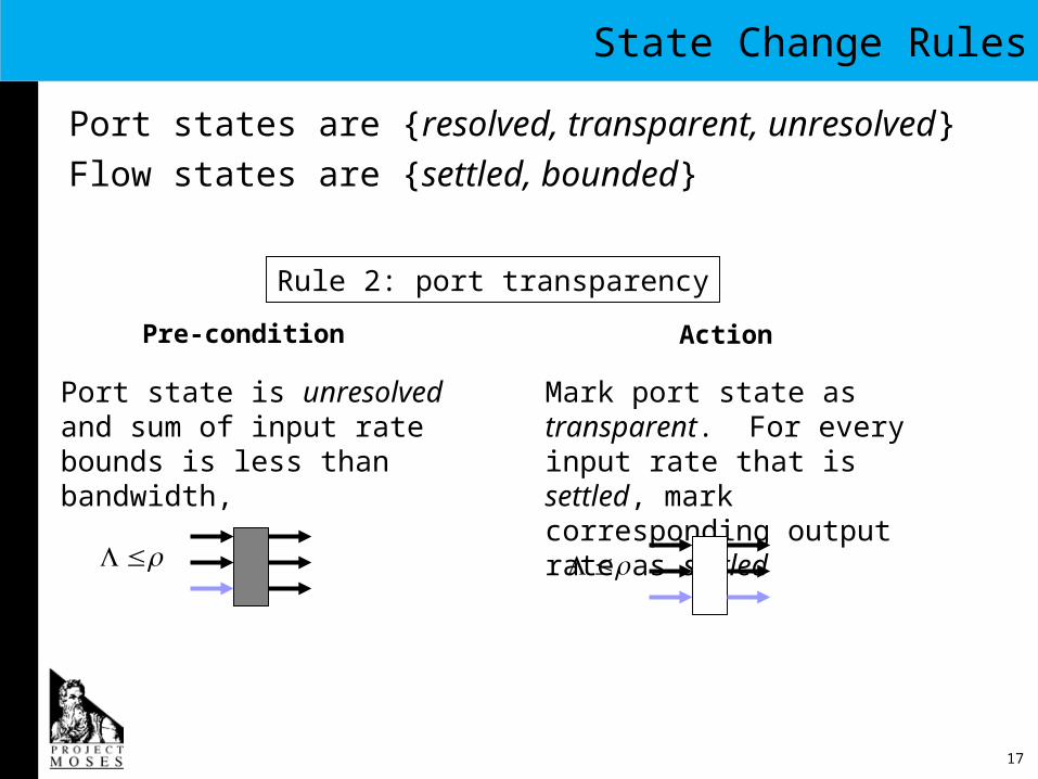
Port states are {resolved, transparent, unresolved}Flow states are {settled, bounded}
Rule 1: port resolution
Pre-condition Action
Port state is not resolved and all input flow states are settled
Mark port state as resolved, compute all output flow values, mark each as settled
17
State Change Rules
Port states are {resolved, transparent, unresolved}Flow states are {settled, bounded}
Rule 2: port transparency
Pre-condition Action
Port state is unresolved and sum of input rate bounds is less than bandwidth,
Mark port state as transparent. For every input rate that is settled, mark corresponding output rate as settled
€
Λ≤ρ
€
Λ ≤ρ
18
State Change Rules
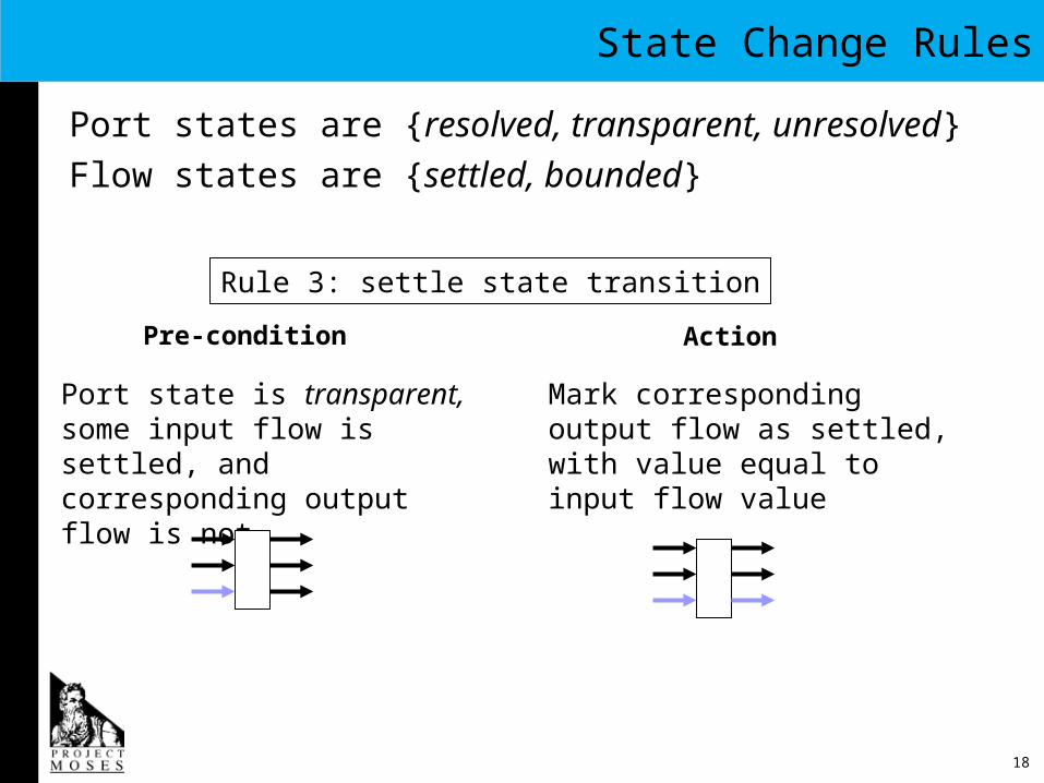
Port states are {resolved, transparent, unresolved}Flow states are {settled, bounded}
Rule 3: settle state transition
Pre-condition Action
Port state is transparent, some input flow is settled, and corresponding output flow is not
Mark corresponding output flow as settled, with value equal to input flow value
19
State Change Rules
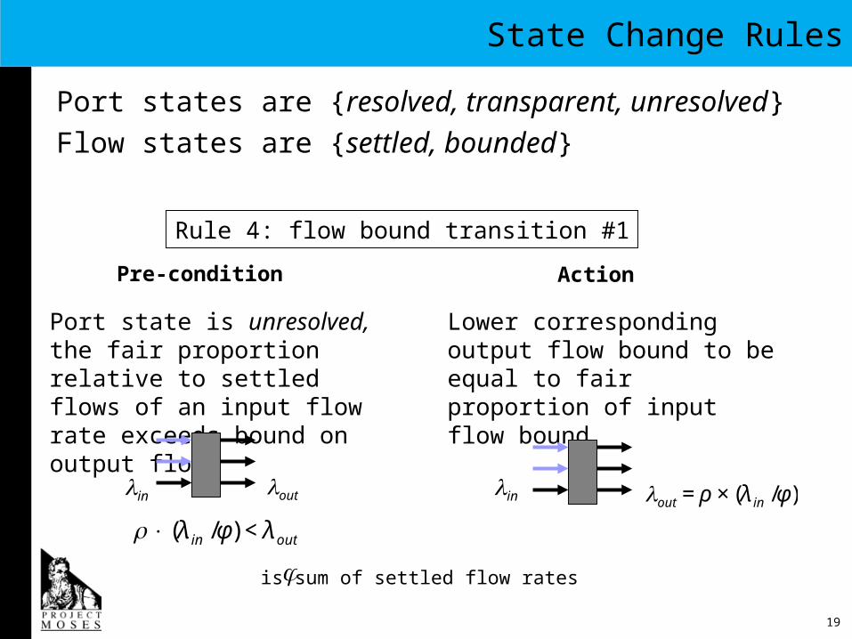
Port states are {resolved, transparent, unresolved}Flow states are {settled, bounded}
Rule 4: flow bound transition #1
Pre-condition Action
Port state is unresolved, the fair proportion relative to settled flows of an input flow rate exceeds bound on output flow
Lower corresponding output flow bound to be equal to fair proportion of input flow bound
€
λin
€
λout
€
ρ×(λ in /φ) < λ out
€
λin
€
λout = ρ × (λ in /φ)
€
φ is sum of settled flow rates
20
State Change Rules
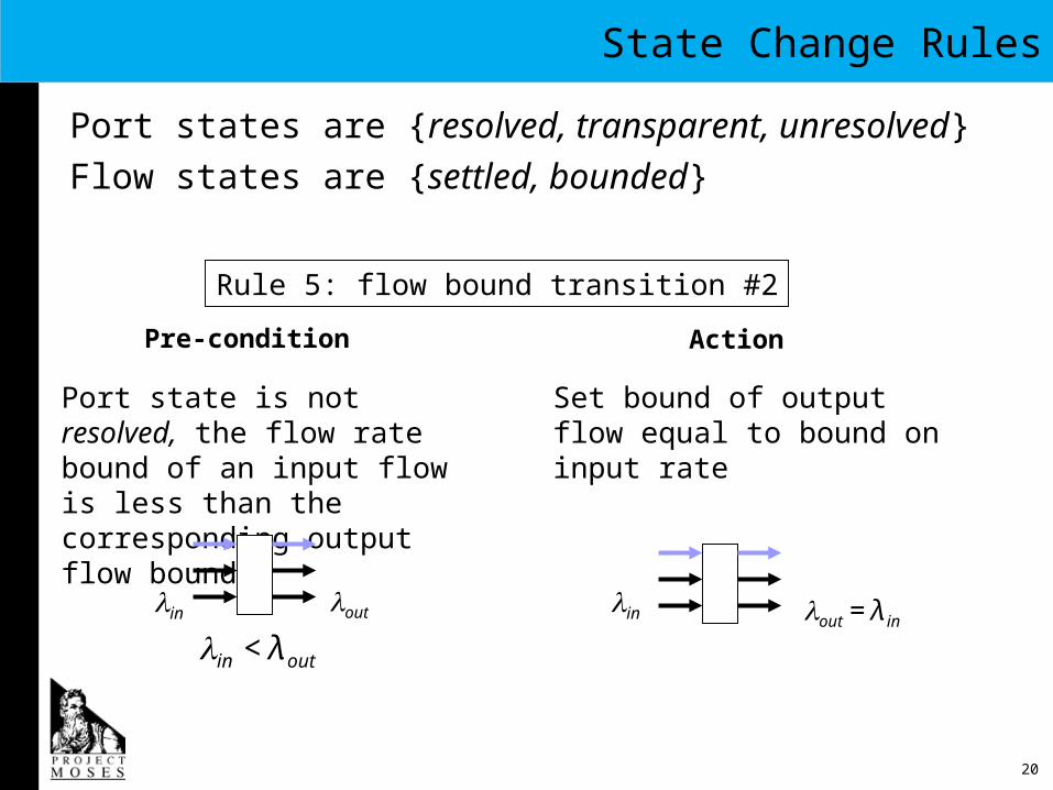
Port states are {resolved, transparent, unresolved}Flow states are {settled, bounded}
Rule 5: flow bound transition #2
Pre-condition Action
Port state is not resolved, the flow rate bound of an input flow is less than the corresponding output flow bound
Set bound of output flow equal to bound on input rate
€
λin
€
λout
€
λin
€
λout = λ in
€
λin < λ out
21
Cycle Resolution
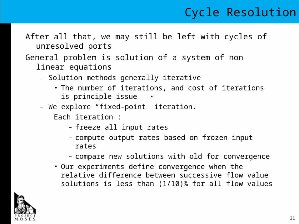
After all that, we may still be left with cycles of unresolved ports
General problem is solution of a system of non-linear equations– Solution methods generally iterative
• The number of iterations, and cost of iterations is principle issue
– We explore “fixed-point” iteration.Each iteration :
– freeze all input rates– compute output rates based on frozen input rates– compare new solutions with old for convergence
• Our experiments define convergence when the relative difference between successive flow value solutions is less than (1/10)% for all flow values
22
Results
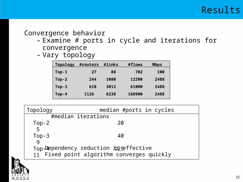
Convergence behavior– Examine # ports in cycle and iterations for
convergence– Vary topology
Topology #routers #links #flows Mbps
Top-1 27 88 702 100
Top-2 244 1080 12200 2488
Top-3 610 3012 61000 2488
Top-4 1126 6238 168900 2488
Topology median #ports in cycles #median iterations Top-2 20 5 Top-3 40 9 Top-4 125 11
Dependency reduction is effectiveFixed point algorithm converges quickly
23
Results
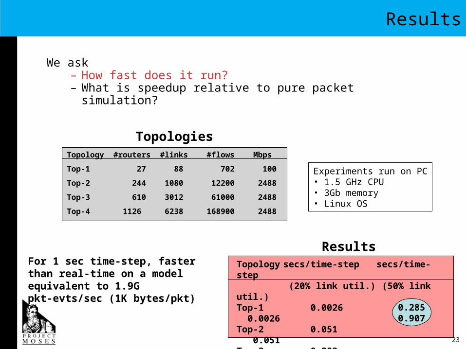
We ask– How fast does it run?– What is speedup relative to pure packet simulation?
Topology #routers #links #flows Mbps
Top-1 27 88 702 100
Top-2 244 1080 12200 2488
Top-3 610 3012 61000 2488
Top-4 1126 6238 168900 2488
Topology secs/time-step secs/time-step (20% link util.) (50% link util.)
Top-1 0.0026 0.0026Top-2 0.051 0.051Top-3 0.283 0.285Top-4 0.852 0.907
For 1 sec time-step, faster than real-time on a model equivalent to 1.9G pkt-evts/sec (1K bytes/pkt)
Experiments run on PC• 1.5 GHz CPU• 3Gb memory• Linux OS
Topologies
Results
0.2850.907
24
Results
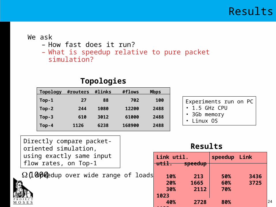
We ask– How fast does it run?– What is speedup relative to pure packet simulation?
Topology #routers #links #flows Mbps
Top-1 27 88 702 100
Top-2 244 1080 12200 2488
Top-3 610 3012 61000 2488
Top-4 1126 6238 168900 2488
Experiments run on PC• 1.5 GHz CPU• 3Gb memory• Linux OS
Topologies
ResultsLink util. speedup Link util. speedup
10% 213 50% 3436 20% 1665 60% 3725 30% 2112 70% 1023 40% 2728 80% 1135
Directly compare packet-oriented simulation, using exactly same input flow rates, on Top-1
€
Ω(1000) speedup over wide range of loads
25
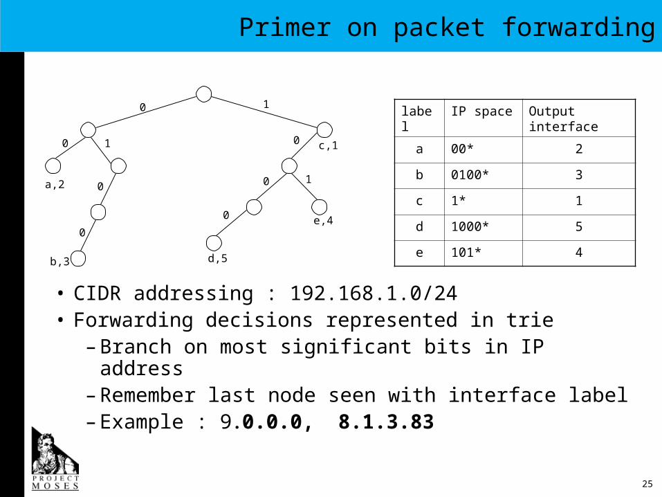
Primer on packet forwarding
• CIDR addressing : 192.168.1.0/24• Forwarding decisions represented in trie
– Branch on most significant bits in IP address– Remember last node seen with interface label– Example : 9.0.0.0, 8.1.3.83
b,3
a,2
c,1
e,4
d,5
0
0
0
0
0
0 1
1
1
0
label IP space Output interface
a 00* 2
b 0100* 3
c 1* 1
d 1000* 5
e 101* 4
26
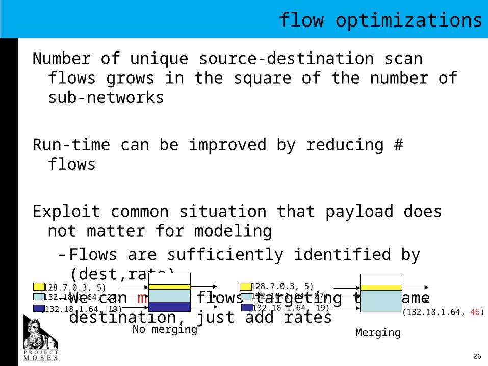
flow optimizations
Number of unique source-destination scan flows grows in the square of the number of sub-networks
Run-time can be improved by reducing # flows
Exploit common situation that payload does not matter for modeling– Flows are sufficiently identified by (dest,rate)– We can merge flows targeting the same
destination, just add rates(128.7.0.3, 5)(132.18.1,64, 27)
(132.18.1.64, 19)
No merging
(128.7.0.3, 5)(132.18.1.64, 27)
(132.18.1.64, 19) (132.18.1.64, 46)
Merging
27
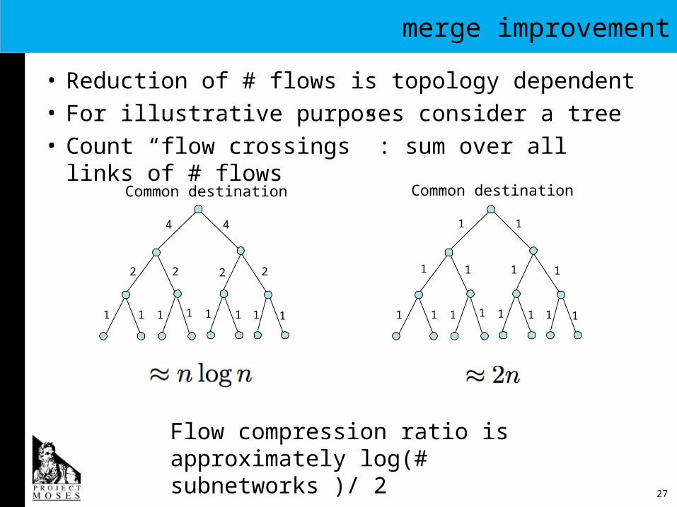
merge improvement
• Reduction of # flows is topology dependent• For illustrative purposes consider a tree• Count “flow crossings” : sum over all links of #
flowsCommon destination
1 1 1 1 1 1 1 1
2 2 2
4
2
4
Common destination
1 1 1 1 1 1 1 1
1 1 1 1
1 1
Flow compression ratio is approximately log(# subnetworks )/ 2
28
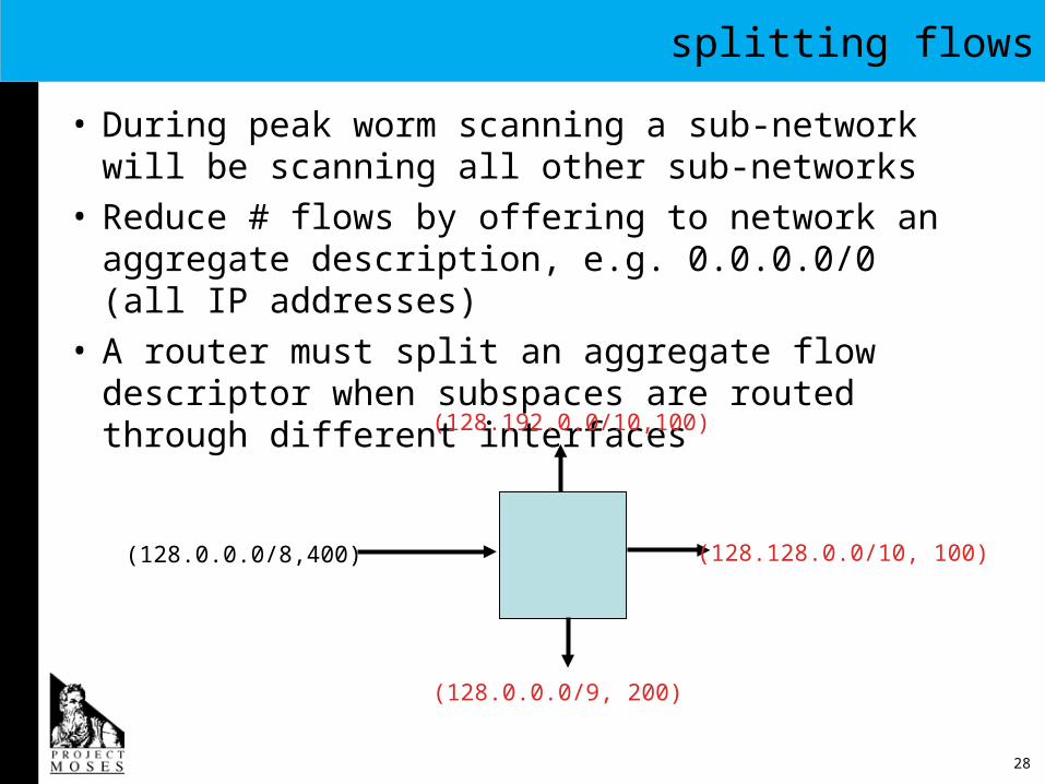
splitting flows
• During peak worm scanning a sub-network will be scanning all other sub-networks
• Reduce # flows by offering to network an aggregate description, e.g. 0.0.0.0/0 (all IP addresses)
• A router must split an aggregate flow descriptor when subspaces are routed through different interfaces
(128.0.0.0/8,400)
(128.192.0.0/10,100)
(128.128.0.0/10, 100)
(128.0.0.0/9, 200)
29
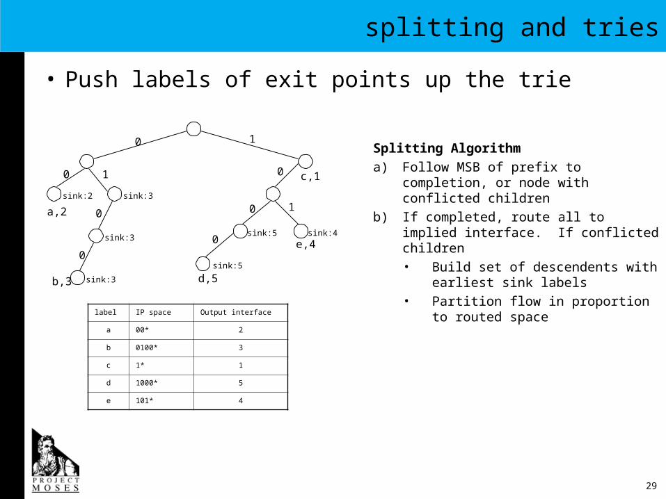
splitting and tries
• Push labels of exit points up the trie
b,3
a,2
c,1
e,4
d,5
0
0
0
0
0
0 1
1
1
0
sink:3
sink:2
sink:3
sink:3
sink:5
sink:5 sink:4
label IP space Output interface
a 00* 2
b 0100* 3
c 1* 1
d 1000* 5
e 101* 4
Splitting Algorithma) Follow MSB of prefix to
completion, or node with conflicted children
b) If completed, route all to implied interface. If conflicted children• Build set of descendents with
earliest sink labels• Partition flow in proportion to
routed space
30
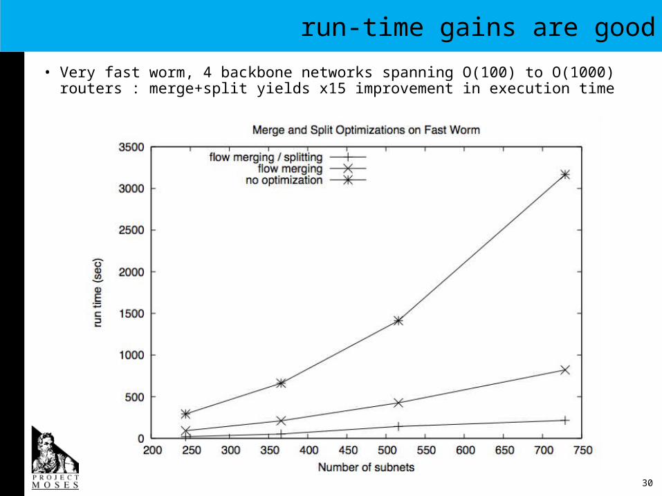
run-time gains are good
• Very fast worm, 4 backbone networks spanning O(100) to O(1000) routers : merge+split yields x15 improvement in execution time
31
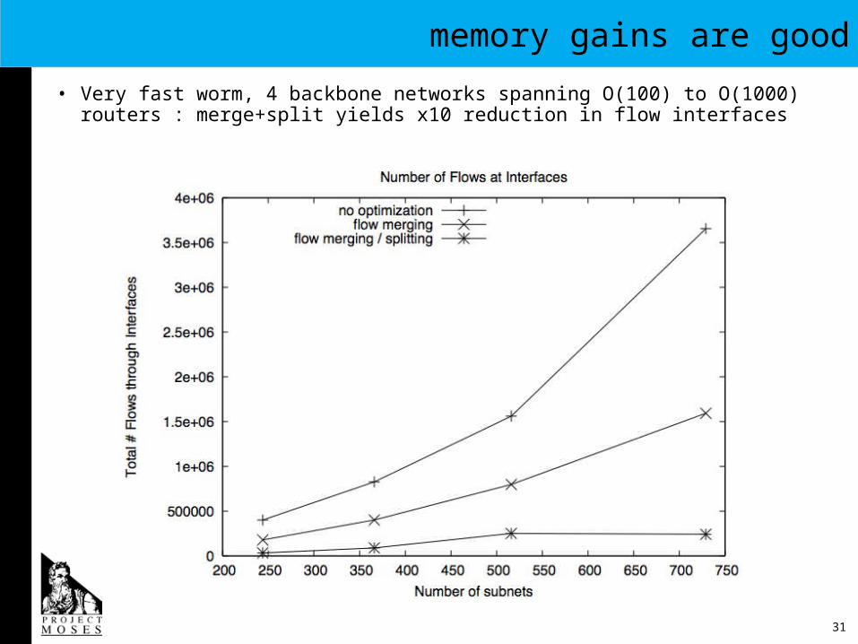
memory gains are good
• Very fast worm, 4 backbone networks spanning O(100) to O(1000) routers : merge+split yields x10 reduction in flow interfaces
32
summary
• Developed hybrid model of worm whose execution time is optimal subject to constraint on error in variance
• Consider backbone + sub-networks model– Developed fast solution for solving huge
system of coupled non-linear equations describing bandwidth sharing
– Developed optimizations that reduce # flows managed in backbone by an order of magnitude
• We are simulating the interactions of infrastructure and worms on very large examples