Embed Size (px)
DESCRIPTION
deadlock, synchronisation, scalability
Citation preview

Sri ManakulaVinayagar Engineering College, Puducherry
Department of Computer Science and Engineering
Subject Name: HIGH PERFORMANCE COMPUTING Subject Code: CS T82
Prepared By :Mr.B.Thiyagarajan,AP/CSEMr.D.Saravanan, AP/CSE
Verified by : Approved by :
UNIT – 1
Introduction: Need of high speed computing Increase the speed of computers History of parallel computers and recent parallel computers; Solving problems in parallel Temporal parallelism Data parallelism Comparison of temporal and data parallel processing Data parallel processing with specialized processors Inter-task dependency. The need for parallel computers Models of computation Analyzing algorithms Expressing algorithms.
TWO MARKS
1. What is high performance computing?
High Performance Computing most generally refers to the practice of aggregating computing power
in a way that delivers much higher performance than one could get out of a typical desktop computer
or workstation in order to solve large problems in science, engineering, or business.
2. Define Computing.
The process of utilizing computer technology to complete a task.
Computing may involve computer hardware and/or software, but must involve some form of a
computer system.
Most individuals use some form of computing every day whether they realize it or not.
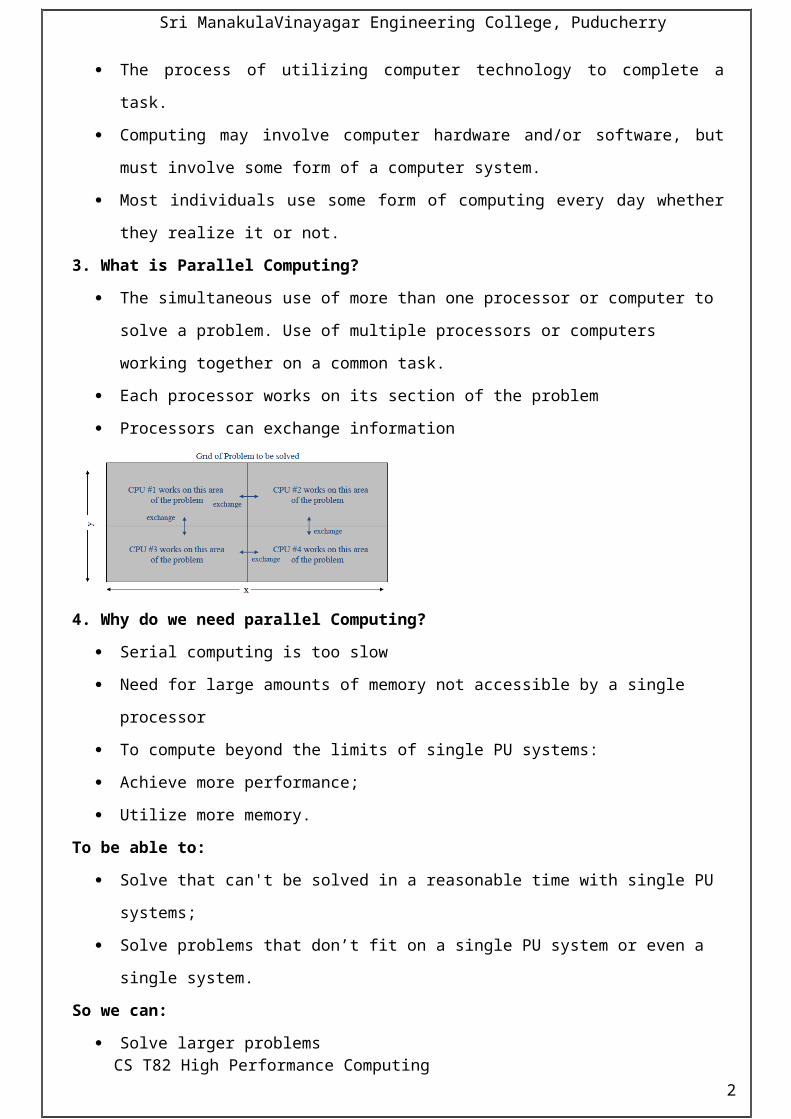
3. What is Parallel Computing?
The simultaneous use of more than one processor or computer to solve a problem. Use of
multiple processors or computers working together on a common task.
Each processor works on its section of the problem
CS T82 High Performance Computing 1
Sri ManakulaVinayagar Engineering College, Puducherry
Processors can exchange information
4. Why do we need parallel Computing?
Serial computing is too slow
Need for large amounts of memory not accessible by a single processor
To compute beyond the limits of single PU systems:
Achieve more performance;
Utilize more memory.
To be able to:
Solve that can't be solved in a reasonable time with single PU systems;
Solve problems that don’t fit on a single PU system or even a single system.
So we can:
Solve larger problems
Solve problems faster
Solve more problems
5. Why parallel Processing?
Single core performance growth has slowed.
More cost-effective to add multiple cores.
6. Write Limits of Parallel Computing.
Theoretical Upper Limits:
Amdahl's Law.
Gustafson’s Law
Practical Limits
Load Balancing.
Non-computational sections.
Other considerations:
Time to develop/rewrite code.
Time do debug and optimize code
7. How to Classify Shared and Distributed Memory?
CS T82 High Performance Computing 2

Sri ManakulaVinayagar Engineering College, Puducherry
All processors have access to a pool of
shared memory
Memory is local to each processor
Access times vary from CPU to CPU
in NUMA systems
Data exchange by message passing
over a network
Example: SGI Altix, IBM P5 nodes Example: Clusters with single-socket
blades
8. Define Hybrid system
A limited number, N, of processors have access to a common pool of shared memory
To use more than N processors requires data exchange over a network
Example: Cluster with multi-socket blades
9. Define Multi Core Systems.
Extension of hybrid model
Communication details increasingly complex
Cache access
Main memory access
Quick Path / Hyper Transport socket connections
Node to node connection via network
10. Define Accelerated Systems
Calculations made in both CPU and accelerator
Provide abundance of low-cost flops
Typically communicate over PCI-e bus
Load balancing critical for performance
CS T82 High Performance Computing 3

Sri ManakulaVinayagar Engineering College, Puducherry
11. What is data parallelism? (Apr2013)
Data parallelism is a form of parallelization of computing across multiple processors in parallel
computing environments. Data parallelism focuses on distributing the data across different parallel
computing nodes. It contrasts to task parallelism as another form of parallelism.
12. Define Stored Program Concept.
Memory is used to store both program and data instructions
Program instructions are coded data which tell the computer to do something
Data is simply information to be used by the program
A central processing unit (CPU) gets instructions and/or data from memory, decodes the
instructions and then sequentially performs them.
13. What is Parallel Computing?(April 2013)
Parallel computing is the simultaneous use of multiple compute resources to solve a computational
problem. The compute resources can include:
A single computer with multiple processors;
An arbitrary number of computers connected by a network;
A combination of both.
14. Why we use Parallel Computing?
There are two primary reasons for using parallel computing:
Save time - wall clock time
Solve larger problems
15. Why do we need high speed Parallel Computing?
The traditional scientific paradigm is first to do theory (say on paper), and then lab experiments to
confirm or deny the theory. The traditional engineering paradigm is first to do a design (say on
CS T82 High Performance Computing 4

Sri ManakulaVinayagar Engineering College, Puducherry
paper), and then build a laboratory prototype. Both paradigms are being replacing by numerical
experiments and numerical prototyping. There are several reasons for this.
1. Real phenomena are too complicated to model on paper (eg. climate prediction).
2. Real experiments are too hard, too expensive, too slow, or too dangerous for a laboratory (eg
oil reservoir simulation, large wind tunnels, overall aircraft design, galactic evolution, whole
factory or product life cycle design and optimization, etc.).
16. How do we increase the speed of Parallel Computers?
We can increase the speed of computers in several ways.
By increasing the speed of the processing element using faster semiconductor technology (by
using advanced technology)
By architecture methods. It in turn we can increase the speed of computer by applying
parallelism.
Use parallelism in Single processor
Overlap the execution of number of instructions by pipelining or by using multiple functional
units
Overlap the operation of different units.
Use parallelism in the problem
Use number of interconnected processors to work cooperatively to solve the problem.
17. Define Temporal Parallelism?
Use parallelism in Single processor. Temporal means Pertaining to time.
Overlap the execution of number of instructions by pipelining or by using multiple functional
units
Overlap the operation of different units.
18. State the advantages & Disadvantages of temporal Parallelism?
Synchronization: Identical time
Bubbles in pipeline Bubbles are formed
Fault tolerance: does not tolerate.
Inter task communication small
Scalability: Can’t be increased.
19. State the advantages & Disadvantages of Data Parallelism?
Advantages:
No Synchronization:
No Bubbles in pipeline
More Fault tolerance
No communication
Disadvantages:
CS T82 High Performance Computing 5
Sri ManakulaVinayagar Engineering College, Puducherry
Static assignment
Partitionable
Time to divide jobs is small.
20. Define Data Parallelism?
Use parallelism in the problem: use number of interconnected processors to work
cooperatively to solve the problem. Here input is divided into some set of jobs and each job is given
to one Processor and works simultaneously.
21. Define Inter task Dependency?
The following assumptions are made in evolving tasks to teacher:
The answer to a question is independent of answers to other questions
Teachers do not have to interact
The same instructions are used to grad all answer books
Tasks are inter related. Some tasks are done independently and simultaneously while others
have to wait for completion of previous tasks.
22. What is parallel Computer? (Apr 2013)
Parallel computing is a form of computation in which many calculations are carried out
simultaneously, operating on the principle that large problems can often be divided into smaller ones,
which are then solved concurrently.
23. Comparison Between Temporal and Data Parallelism. (November 2013)
TEMPORAL PARALLELISM DATA PARALLELISM
Independent task
Tasks take equal time
Bubbles leads to idling
Task assignment is static
Not tolerant to processor
Efficient with fine grained
Full jobs are assigned
Tasks take different time
No bubbles
Task assignment is static,
dynamic or quasi dynamic
Tolerates to processor
Efficient with coarse grained
11 Marks
1. What is Parallel Computing and explain?
Additionally, software has been written for serial computation:
To be executed by a single computer having a single Central Processing Unit (CPU);
Problems are solved by a series of instructions, executed one after the other by the CPU. Only
one instruction may be executed at any moment in time.
CS T82 High Performance Computing 6

Sri ManakulaVinayagar Engineering College, Puducherry
In the simplest sense, parallel computing is the simultaneous use of multiple compute
resources to solve a computational problem.
The compute resources can include:
A single computer with multiple processors;
An arbitrary number of computers connected by a network;
A combination of both.
The computational problem usually demonstrates characteristics such as the ability to be:
Broken apart into discrete pieces of work that can be solved simultaneously;
Execute multiple program instructions at any moment in time;
Solved in less time with multiple compute resources than with a single compute resource.
Parallel computing is an evolution of serial computing that attempts to emulate what has
always been the state of affairs in the natural world: many complex, interrelated events
happening at the same time, yet within a sequence. Some examples:
Planetary and galactic orbits
Weather and ocean patterns
Tectonic plate drift
Rush hour traffic in LA
Automobile assembly line
Daily operations within a business
Building a shopping mall
Ordering a hamburger at the drive through.
Traditionally, parallel computing has been considered to be "the high end of computing" and
has been motivated by numerical simulations of complex systems and "Grand Challenge
Problems" such as:
weather and climate
chemical and nuclear reactions
biological, human genome
geological, seismic activity
mechanical devices - from prosthetics to spacecraft
electronic circuits
manufacturing processes
CS T82 High Performance Computing 7

Sri ManakulaVinayagar Engineering College, Puducherry
Today, commercial applications are providing an equal or greater driving force in the
development of faster computers. These applications require the processing of large amounts
of data in sophisticated ways. Example applications include:
parallel databases, data mining
oil exploration
web search engines, web based business services
computer-aided diagnosis in medicine
management of national and multi-national corporations
advanced graphics and virtual reality, particularly in the entertainment industry
networked video and multi-media technologies
collaborative work environments
Ultimately, parallel computing is an attempt to maximize the infinite but seemingly scarce
commodity called time.
2. Why do we need Use Parallel Computing? (April 2013)
There are two primary reasons for using parallel computing:
Save time - wall clock time
Solve larger problems
Other reasons might include:
Taking advantage of non-local resources - using available compute resources on a wide
area network, or even the Internet when local compute resources are scarce.
Cost savings - using multiple "cheap" computing resources instead of paying for time on a
supercomputer.
Overcoming memory constraints - single computers have very finite memory resources.
For large problems, using the memories of multiple computers may overcome this
obstacle.
Limits to serial computing - both physical and practical reasons pose significant
constraints to simply building ever faster serial computers:
Transmission speeds - the speed of a serial computer is directly dependent upon how fast
data can move through hardware. Absolute limits are the speed of light (30
cm/nanosecond) and the transmission limit of copper wire (9 cm/nanosecond). Increasing
speeds necessitate increasing proximity of processing elements.
CS T82 High Performance Computing 8

Sri ManakulaVinayagar Engineering College, Puducherry
Limits to miniaturization - processor technology is allowing an increasing number of
transistors to be placed on a chip. However, even with molecular or atomic-level
components, a limit will be reached on how small components can be.
Economic limitations - it is increasingly expensive to make a single processor faster.
Using a larger number of moderately fast commodity processors to achieve the same (or
better) performance is less expensive.
The future: during the past 10 years, the trends indicated by ever faster networks,
distributed systems, and multi-processor computer architectures (even at the desktop level)
suggest that parallelism is the future of computing
3. What is the Need of high speed computing?
The traditional scientific paradigm is first to do theory (say on paper), and then lab
experiments to confirm or deny the theory.
The traditional engineering paradigm is first to do a design (say on paper), and then build a
laboratory prototype.
Both paradigms are being replacing by numerical experiments and numerical prototyping.
There are several reasons for this.
Real phenomena are too complicated to model on paper (eg. climate prediction).
Real experiments are too hard, too expensive, too slow, or too dangerous for a laboratory (eg
oil reservoir simulation, large wind tunnels, overall aircraft design, galactic evolution, whole
factory or product life cycle design and optimization, etc.).
Scientific and engineering problems requiring the most computing power to simulate are
commonly called "Grand Challenges like predicting the climate 50 years hence, are estimated
to require computers computing at the rate of 1 Tflop = 1 Teraflop = 10^12 floating point
operations per second, and with a memory size of 1 TB = 1 Terabyte = 10^12 bytes. Here is
some commonly used notation we will use to describe problem sizes:
1 Mflop = 1 Megaflop = 10^6 floating point operations per second
1 Gflop = 1 Gigaflop = 10^9 floating point operations per second
1 Tflop = 1 Teraflop = 10^12 floating point operations per second
1 MB = 1 Megabyte = 10^6 bytes
1 GB = 1 Gigabyte = 10^9 bytes
1 TB = 1 Terabyte = 10^12 bytes
1 PB = 1 Petabyte = 10^15 bytes
4. How do we Increase the speed of Computers.
We can increase the speed of computers in several ways.
CS T82 High Performance Computing 9

Sri ManakulaVinayagar Engineering College, Puducherry
By increasing the speed of the processing element using faster semiconductor technology (by using advanced technology)
By architecture methods. It in turn we can increase the speed of computer by applying parallelism.
Use parallelism in Single processor
overlap the execution of number of instructions by pipelining or by using multiple
functional units
Overlap the operation of different units.
Use parallelism in the problem
Use number of interconnected processors to work cooperatively to solve the problem.
5. Describe about History of parallel computers: A brief history of parallel computers are
given below
VECTOR SUPERCOMPUTERS:
Glory days: 76-90 Famous examples: Cray machines
Characterized by:
The fastest clock rates, because vector pipelines can be very simple.
Vector processing.
Quite good vectorizing compilers.
High price tag; small market share.
Not always scalable because of shared-memory bottleneck (vector processors need more data
per cycles than conventional processors). Vector processing is back in various forms: SIMD
extensions of commodity microprocessors (e.g. Intel's SSE), vector processors for game
consoles (Cell), multithreaded vector processors (Cray), etc.
Vector processors went down temporarily because of:
Market issues, price/performance, microprocessor revolution, commodity microprocessors.
Not enough parallelism for biggest problems. Hard to vectorize/parallelize automatically
Didn't scale down.
MPPs
Glory days: 90-96
Famous examples: Intel hypercubes and Paragon, TMC Connection Machine, IBM SP,
Cray/SGI T3E.
CS T82 High Performance Computing 10

Sri ManakulaVinayagar Engineering College, Puducherry
Characterized by:
Scalable interconnection network, up to 1000's of processors. We'll discuss these networks
shortly
Commodity (or at least, modest) microprocessors.
Message passing programming paradigm.
Killed by:
Small market niche, especially as a modest number of processors can do more and more.
Programming paradigm too hard.
Relatively slow communication (especially latency) compared to ever-faster processors (this
is actually no more and no less than another example of the memory wall).
Today
A state of flux in hardware.
But more stability in software, e.g., MPI and OpenMP.
Machines are being sold, and important problems are being solved, on all of the following:
Vector SMPs, e.g., Cray X1, Hitachi, Fujitsu, NEC.
SMPs and ccNUMA, e.g., Sun, IBM, HP, SGI, Dell, hundreds of custom boxes.
Distributed memory multiprocessors, e.g., Cray XT3, IBM Blue Gene.
Clusters: Beowulf (Linux) and many manufacturers and assemblers.
A complete top-down view: At the highest level you have either a distributed memory
architecture with a scalable interconnection network, or an SMP architecture with a bus.
A distributed memory architecture may or may not provide support for a global memory
consistency model (such as cache coherence, software distributed shared memory, coherent
RDMA, etc.). On an SMP architecture you expect hardware support for cache coherence.
A distributed memory architecture can be built from SMP or even (rarely) ccNUMA boxes.
Each box is treated as a tightly coupled node (with local processors and uniformly accessed
shared memory). Boxes communicate via message passing, or (less frequently) with hardware
or software memory coherence schemes. Both on distributed and on shared memory
architectures, the processors themselves may support an internal form of task or data
parallelism. Processors may be vector processors, commodity microprocessors with multiple
cores, or multiple threads multiplexed over a single core, heterogeneous multicore processors,
etc.
Programming: Typically MPI is supported over both distributed and shared-memory
substrates for portability (large existing base of code written and optimized in MPI). OpenMP
CS T82 High Performance Computing 11

Sri ManakulaVinayagar Engineering College, Puducherry
and POSIX threads are almost always available on SMPs and ccNUMA machines. OpenMP
implementations over distributed memory machines with software support for cache
coherence also exist, but scaling these implementation is hard and is a subject of ongoing
research.
Future
The end of Moore's Law?
Nanoscale electronics
Exotic architectures? Quantum, DNA/molecular. 6. Explain various methods for solving problems in parallel.
Method 1: Utilizing temporal parallelism
Solving a simple job can be solved in parallel in many ways.
Consider there are 1000 who appeared for the exam. There are 4 questions in each answer book. If a
teacher is to correct these answer books, the following instructions are given to them.
1. Take an answer book from the pile of answer books.
2. Correct the answer to Q1,namely A1.
3. Repeat step 2 for answers to Q2,Q3,Q4 namely A2,A3,A4.
4. Add marks.
5. Put answer book in pile of corrected answer books.
6. Repeat steps 1 to 5 until no answer books are left.
Ask 4 teachers to correct each answer book by sitting in one line.
The first teacher corrects answer Q1,namely A1 of first paper and passes the paper to the
second teacher.
When the first three papers are corrected, some are idle.
Time taken to correct A1=Time to correct A2= Time to correct A3= Time to correct A4=5
minutes. Then first answer book takes 20 min.
Total time taken to correct 1000 papers will be 20+(999*5)=5015 min.This is about 1/4th of
the time taken.
Temporal means pertaining to time.
The method is correct if:
Jobs are identical.
Independent tasks are possible.
Time is same.
No. of tasks is small compared to total no of jobs.
CS T82 High Performance Computing 12

Sri ManakulaVinayagar Engineering College, Puducherry
Let no of jobs=n
Time to do a job=p
Each job is divided into k tasks
Time for each task=p/k
Time to complete n jobs with no pipeline processing =np
Time complete n jobs with pipeline processing of k teachers=p+(n-1)p/k=p*[(k+n-1)/k]
Speedup due to pipeline processing=[np/p(k+n-1)/k]=[k/1+(k-1)/n]
Problems encountered:
Synchronization:
Identical time
Bubbles in pipeline
Bubbles are formed
Fault tolerance
Does not tolerate.
Inter task communication
small
Scalability
Cant be increased.
Method 2: Utilizing Data Parallelism
Divide the answer books into four piles and give one pile to each teacher.
Each teacher takes 20 min to correct an answer book, the time taken for 1000 papers is
5000 min.
Each teacher corrects 250 papers but simultaneously.
Let no of jobs=n
Time to do a job=p
Let there be k teachers
Time to distribute=kq
Time to complete n jobs by single teacher=np
Time to complete n jobs by k teachers=kq+np/k
Speed up due to parallel processing=np/kq+np/k=knp/k8k*q+np=k/1+(kq/np)
Advantages:
No Synchronization:
No Bubbles in pipeline
More Fault tolerance
No communication
Disadvantages:
CS T82 High Performance Computing 13

Sri ManakulaVinayagar Engineering College, Puducherry
Static assignment
Partitionable
Time to divide jobs is small
METHOD 3: Combined Temporal and Data Parallelism:
Combining method 1 and 2 gives this method.
Two pipelines of teachers are formed and each pipeline is given half of total no of jobs.
Halves the time taken by single pipeline.
Reduces time to complete set of jobs.
Very efficient for numerical computing in which a no of long vectors and large matrices are
used as data and could be processed.
METHOD 4: Data Parallelism With Dynamic Assignment
A head examiner gives one answer book to each teacher.
All teachers simultaneously correct the paper.
A teacher who completes goes to head examiner for another paper.
If second completes at the same time, then he queues up in front of head examiner.
Advantages:
Balancing of the work assigned to each teacher.
Teacher is not forced to be idle.
No bubbles
Overall time is minimized
Disadvantages:
Teachers Have To Wait In The Queue.
Head examiner can become bottle neck
Head examiner is idle after handing the papers.
Difficult to increase the number of teachers
If speedup of a method is directly proportional to the number, then the method is said to scale well.
Let total no of papers=n
Let there be k teachers
Time waited to get paper=q
Time for each teacher to get, grade and return a paper=(q+p)
Total time to correct papers by k teachers=[n(q+p)/k]
Speed up due to parallel processing=np/[n(q+p)/k]=k/[1+(q/p)]
METHOD 5: Data Parallelism with Quasi-Dynamic Scheduling
CS T82 High Performance Computing 14
Sri ManakulaVinayagar Engineering College, Puducherry
Method 4 can be made better by giving each teacher unequal sets of papers to correct. Teacher 1,2,3,4
may be given with 7, 9, 11, 13 papers. When finish that further papers will be given. This randomizes
the job completion and reduces the probability of queue. Each job is much smaller compared to the
time to actually do the job. This method is in between purely static and purely dynamic schedule. The
jobs are coarser grain in the sense that a bunch of jobs are assigned and the completion time will be
more than if one job is assigned.
Comparison between temporal and data parallelism:
TEMPORAL PARALLELISM DATA PARALLELISM
Independent task
Tasks take equal time
Bubbles leads to idling
Task assignment is static
Not tolerant to processor
Efficient with fine grained
Full jobs are assigned
Tasks take different time
No bubbles
Task assignment is static, dynamic
or quasi dynamic
Tolerates to processor
Efficient with coarse grained
Data parallel processing with specialized processor:
Data Parallel Processing is more tolerant but requires each teacher to be capable of correcting
answers to all questions with equal case.
METHOD 6: Specialist Data Parallelism
There is a head examiner who dispatches answer papers to teachers. We assume that teacher 1(T1)
grades A1, teacher 2(T2) grades A2 and teacher i(Ti) grades Ai to question Qi.
Procedure:
Give one answer book to T1,T2,T3,T4
When a corrected answer paper is returned check if all questions are graded. If yes add marks
and put the paper in the output pile.
If no check which questions are not graded
For each I,if Ai is ungraded and teacher Ti is idle send it to teacher Ti or if any other teacher
Tp is idle.
Repeat steps 2,3 and 4 until no answer paper remains in input pile
METHOD 7: Coarse Grained Specialist Temporal Parallelism
All teachers are independently and simultaneously at their pace. That teacher will end up spending a
lot of time inefficiently waiting for other teachers to complete their work.
Procedure:
Answer papers are divided into 4 equal piles and put in the in-trays of each teacher. Each teacher
repeats 4 times simultaneously steps 1 to 5.
CS T82 High Performance Computing 15

Sri ManakulaVinayagar Engineering College, Puducherry
For teachers Ti(i=1 to 4) do in parallel
Take an answer paper from in-tray
Grade answer Ai to question Qi and put in out-tray
Repeat steps 1 and 2 till no papers are left
Check if teacher (i+1)mod4’s in-tray is empty.
As soon as it is empty, empty own out-tray into in-tray of that teacher.
METHOD 8: Agenda Parallelism
Answer book is thought as an agenda of questions to be graded. All teachers are asked to work on the
first item on agenda, namely grade the answer to first question in all papers. Head examiner gives one
paper to each teacher and asks him to grade the answer A1 to Q1.When a teacher finishes this, he is
given with another paper. This is data parallel method with dynamic schedule and fine grain tasks.
7. Briefly explain about Inter Task Dependency with example
The following assumptions are made in evolving tasks to teacher:
The answer to a question is independent of answers to other questions
Teachers do not have to interact
The same instructions are used to grad all answer books
Tasks are inter related. Some tasks are done independently and simultaneously while others have to
wait for completion of previous tasks. The inter relations of various tasks of a job may be represented
graphically as a task graph.
Procedure: Recipe for Chinese vegetable fried rice:
T1: Clean and wash rice
T2: Boil water in a vessel with 1 teaspoon salt
T3: Put rice in boiling water with some oil and cook till soft
T4: Drain rice and cool
T5: Wash and scrape carrots
T6: Wash and string French beans
T7: Boil water with ½ teaspoon salt in 2 vessels
T8: Drop carrots and French beans in boiling water
T9: Drain and cool carrots and French beans
T10: Dice carrots
T11: Dice French beans
T12: Peel onions and dice into small pieces
T13: Clean cauliflower .Cut into small pieces.
T14: Heat oil in iron pan and fry diced onion cauliflower for 1 min in heated oil
T15: Add diced carrots and French beans to above and fry for 2 min.
T16: Add cooled cooked rice, chopped onions and soya sauce to the above and stir and fry for 5 min.
CS T82 High Performance Computing 16

Sri ManakulaVinayagar Engineering College, Puducherry
There are 16 tasks in this, in that they have to be carried out in sequence. A graph showing the
relationship among the tasks is given
8. Explain the Various Computation Models? (November 2013)
RAM
PRAM (parallel RAM)
Interconnection Network
Combinatorial Circuits
Parallel and Distributed Computation
Many interconnected processors working concurrently
Connection machine
Internet
Types of multiprocessing frameworks
Parallel
Distributed
Technical aspects
Parallel computers (usually) work in tight syncrony, share memory to a large extent and have
a very fast and reliable communication mechanism between them.
Distributed computers are more independent, communication is less Frequent and less
synchronous, and the cooperation is limited.
Purposes
Parallel computers cooperate to solve more efficiently (possibly) Difficult problems
Distributed computers have individual goals and private activities. Sometime communications
with other ones are needed. (e. G. Distributed data base operations).
The RAM Sequential Model
RAM is an acronym for Random Access Machine
RAM consists of
A memory with M locations.
Size of M can be as large as needed.
A processor operating under the control of a sequential program which can
load data from memory
store date into memory
execute arithmetic & logical computations on data.
A memory access unit (MAU) that creates a path from the processor to an arbitrary
memory location.
RAM Sequential Algorithm Steps
CS T82 High Performance Computing 17

Sri ManakulaVinayagar Engineering College, Puducherry
A READ phase in which the processor reads datum from a memory location and copies it into
a register.
A COMPUTE phase in which a processor performs a basic operation on data from one or two
of its registers.
A WRITE phase in which the processor copies the contents of an internal register into a
memory location.
PRAM (Parallel Random Access Machine)
Let P1, P2 , ... , Pn be identical processors
Each processor is a RAM processor with a private local memory.
The processors communicate using m shared (or global) memory locations, U1, U2, ..., Um.
Allowing both local & global memory is typical in model study.
Each Pi can read or write to each of the m shared memory locations.
All processors operate synchronously (i.e. using same clock), but can execute a different
sequence of instructions.
Some authors inaccurately restrict PRAM to simultaneously executing the same
sequence of instructions (i.e., SIMD fashion)
Each processor has a unique index called, the processor ID, which can be referenced by the
processor’s program.
Often an unstated assumption for a parallel model
Each PRAM step consists of three phases, executed in the following order:
A read phase in which each processor may read a value from shared memory
A compute phase in which each processor may perform basic arithmetic/logical
operations on their local data.
A write phase where each processor may write a value to shared memory.
Note that this prevents reads and writes from being simultaneous.
Above requires a PRAM step to be sufficiently long to allow processors to do different
arithmetic/logic operations simultaneously.
PRAM Memory Access Methods
Exclusive Read (ER): Two or more processors can not simultaneously read the same memory
location.
Concurrent Read (CR): Any number of processors can read the same memory location
simultaneously.
Exclusive Write (EW): Two or more processors can not write to the same memory location
simultaneously.
CS T82 High Performance Computing 18

Sri ManakulaVinayagar Engineering College, Puducherry
Concurrent Write (CW): Any number of processors can write to the same memory location
simultaneously.
Variants for Concurrent Write
Priority CW: The processor with the highest priority writes its value into a memory location.
Common CW: Processors writing to a common memory location succeed only if they write
the same value.
Arbitrary CW: When more than one value is written to the same location, any one of these
values (e.g., one with lowest processor ID) is stored in memory.
Random CW: One of the processors is randomly selected write its value into memory.
UNIT – IQUESTION BANK
TWO MARKS1. What is high performance computing?
2. Define Computing.
3. What is Parallel Computing?
4. Why do we need parallel Computing?
5. Why parallel Processing?
6. Write Limits of Parallel Computing.
7. How to Classify Shared and Distributed Memory?
8. Define Hybrid system
9. Define Multi Core Systems.
10. Define Accelerated Systems
3. What is data parallelism? (Apr 2013)
4. Define Stored Program Concept.
5. What is Parallel Computing? (April 2013)
6. Why we use Parallel Computing?
7. Why do we need high speed Parallel Computing?
8. How do we increase the speed of Parallel Computers?
9. Define Temporal Parallelism?
10. State the advantages & Disadvantages of temporal Parallelism?
11. State the advantages & Disadvantages of Data Parallelism?
12. Define Data Parallelism?
13. Define Inter task Dependency?
14. What is parallel Computer? (Apr 2013)
15. Comparison Between Temporal and Data Parallelism. (November 2013)
CS T82 High Performance Computing 19

Sri ManakulaVinayagar Engineering College, Puducherry
11 Marks
1. What is Parallel Computing and explain?
2. Why do we need Use Parallel Computing? (April 2013) ( Ref.Pg.No.8)
3. What is the Need of high speed computing?
4. How do we Increase the speed of Computers.
5. Describe about History of parallel computers:
6. Explain various methods for solving problems in parallel. (November 2013)(Ref.Pg.No.:12)
7. Briefly explain about Inter Task Dependency with example
8. Explain the Various Computation Models?(November 2013)(Ref.Pg.No.18)
CS T82 High Performance Computing 20

Sri ManakulaVinayagar Engineering College, Puducherry
UNIT – II
Parallel Programming Platforms:
Trends in microprocessor architectures
Limitations of memory system performance
Parallel computing platforms
Communication costs in parallel machines
Routing mechanisms for interconnection networks.
Principles of Parallel Algorithm Design:
Preliminaries
Decomposition techniques
Characteristics of tasks and interactions
Mapping techniques for load balancing
Methods for containing interaction overheads
Parallel algorithm models.
Basic Communication Operations:
One-to-all broadcast and all-to-one reduction
All-to-all broadcast reduction
All-reduce and prefix-sum operations
Scatter and gather
all-to-all personalized communication
Circular shift
Improving the speed of some communication operations.
2 MARKS
1. Write the trends in microprocessor architecture?
A computer is a system which processes data according to a specified algorithm. It contains
One or more programmable (in the sense that the user can specify its operation) digital
processors, also called central processing units (CPUs), memory for storing data and
instructions, and input and output devices.
2. What is the limitation of memory system performance?
The effective performance of a program on a computer relies not just on the speed of the
processor but also on the ability of the memory system to feed data to the processor. At the
logical level, a memory system, possibly consisting of multiple levels of caches, takes in a
request for a memory word and returns a block of data of size b containing the requested word
CS T82 High Performance Computing 21

Sri ManakulaVinayagar Engineering College, Puducherry
after l nanoseconds. Here, l is referred to as the latency of the memory. The rate at which data
can be pumped from the memory to the processor determines the bandwidth of the memory
system.
3. What is the parallel computing platform?
Traditionally, software has been written for serial computation
To be run on a single computer having a single Central Processing Unit (CPU);
A problem is broken into a discrete series of instructions.
Instructions are executed one after another.
Only one instruction may execute at any moment in time.
4. What is the communication cost in parallel machine? (April 2013)
One of the major overheads in the execution of parallel programs arises from communication
of information between processing elements. The cost of communication is dependent on a
variety of features including the programming model semantics, the network topology, data
handling and routing, and associated software protocols
5. What is the Routing mechanism for interconnection networks? (November 2013)
A routing mechanism determines the path a message takes through the network to get from
the source to the destination node. It takes as input a message's source and destination nodes. It
may also use information about the state of the network. It returns one or more paths through
the network from the source to the destination node.
6. Write the characteristics of task and interaction?
Task generation
Task size
Knowledge of task size
Size and data associated with task.
7. What is the mapping technique for load balancing?
Once a computation has been decomposed into tasks, these tasks are mapped onto processes
with the objective that all tasks complete in the shortest amount of elapsed time.
In order to achieve a small execution time, the overheads of executing the tasks in
parallel must be minimized. For a given decomposition, there are two key sources of
overhead.
The time spent in inter-process interaction is one source of overhead. Another
important source of overhead is the time that some processes may spend being idle.
Some processes can be idle even before the overall computation is finished for a
variety of reasons. Uneven load distribution may cause some processes to finish earlier
than others.
CS T82 High Performance Computing 22

Sri ManakulaVinayagar Engineering College, Puducherry
At times, all the unfinished tasks mapped onto a process may be waiting for tasks
mapped onto other processes to finish in order satisfying the constraints imposed by
the task-dependency graph. Both interaction and idling are often a function of
mapping.
Therefore, a good mapping of tasks onto processes must strive to achieve the twin
objectives of (1) reducing the amount of time processes spend in interacting with each
other, and (2) reducing the total amount of time some processes are idle while the others
are engaged in performing some tasks.
8. Write the method for containing interaction overhead?
As noted earlier, reducing the interaction overhead among concurrent tasks is important for an
efficient parallel program. The overhead that a parallel program incurs due to interaction among
its processes depends on many factors, such as the volume of data exchanged during
interactions, the frequency of interaction, the spatial and temporal pattern of interactions, etc.
9. What is the Parallel algorithm model?
In computer science, a parallel algorithm or concurrent algorithm, as opposed to a
traditional sequential (or serial) algorithm, is an algorithm which can be executed a piece at a
time on many different processing devices, and then combined together again at the end to get
the correct result.
10. What is the One to all broadcast and all to one reduction?
Parallel algorithm often requires a single process to send identical data to all other processes
or to subset of them. This operation is known as one to all broadcast. Initially, only the source
process has the data size m that needs to be broadcast. At the termination of the procedure, there
are p copies of the initial data one belonging to each process. The dual of one to all broadcast is
all to one reduction.
11. What is the All to all broadcast and reduction?
All to all broadcast is generalization of one to all broadcast in which all p nodes
simultaneously initiate a broadcast. A process sends the same m-word message to every other
process, but different processes may broadcast different message.
12. Write the types of all to all broadcast reduction?
Ring or linear array
Mesh
Hyper cube
13. What is the Scatter and gather?
In scatter operation a single node sends a unique message of size m to every other node. This
operation is also known as one to all personalized communication. The dual of one to all
personalized communication or the scatter operation is the gather operation.
CS T82 High Performance Computing 23

Sri ManakulaVinayagar Engineering College, Puducherry
14. What is the All to all personalized communication?
In all too all personalized communication each node sends a distinct message of size m to
every other node. Each node sends different messages to different nodes, unlike all to all
broadcast, in which each node send message to all other nodes.
15. Define Circular shift.
Circular shift is a member of a broader class of global communication operation known as
permutation. A permutation is a simultaneous, one to one data redistribution operation in which
node sends a packet of m words to a unique node.
16. Write the types of improving the speed of some communication operation
Splitting and routing message in parts
All port communication
17. Define Decomposition?
The process of dividing a computation into smaller parts, some of all parts which potentially
be executed in parallel, is called as decomposition.
18. What is the Granularity, Concurrency and task generation?
The number and size of task into which a problem is decomposed determines the granularity
of decomposition. Decomposition into a large no of small task is called fine-grained and
decomposition into a small number of large tasks is called as coarse grained.
19. Write the Characteristic of inter task interaction?
Static versus dynamic
Regular versus irregular
Read only versus read writ
One way versus two way
20. Define Recursive decomposition.
Recursive decomposition is a method for inducing concurrency in problem that can be solved
using the divide and conquers strategy.
21. Define Data decomposition.
Data decomposition is a powerful and commonly used method for deriving concurrency in
algorithm that operates on large data structures. In this method the decomposition of
computation is done in two steps. In the first step, the data on which the computations are
performed is portioned and in the second step the data partitioning is used to induce a
partitioning of the computation into task.
22. Define exploratory decomposition.
Exploratory decomposition is used to decompose problems whose underlying computation
corresponds to search of a space for solution.
CS T82 High Performance Computing 24

Sri ManakulaVinayagar Engineering College, Puducherry
23. Define Speculative decomposition.
Speculative decomposition is used when a program may take one of many possible
computationally significant branches depending on the output of other computations that
precede it.
24. Write the types of parallel algorithm model?
Data parallel model
Task graph model
Work pool model
Master-slave model
Pipeline or Producer-Consumer model
Hybrid model
25. Write the Decomposition techniques?
Recursive Decomposition
Exploratory Decomposition
Hybrid Decomposition
CS T82 High Performance Computing 25

Sri ManakulaVinayagar Engineering College, Puducherry
11 MARKS
1. Explain the limitations of memory system performance ( April 2013)
The effective performance of a program on a computer relies not just on the speed of the processor but also on the ability of the memory system to feed data to the processor.
At the logical level, a memory system, possibly consisting of multiple levels of caches, takes in a request for a memory word and returns a block of data of size b containing the requested word after l nanoseconds.
Memory system, and not processor speed, is often the bottleneck for many applications. Memory system performance is largely captured by two parameters, latency and bandwidth. Latency is the time from the issue of a memory request to the time the data is available at the
processor. Bandwidth is the rate at which data can be pumped to the processor by the memory system. It is very important to understand the difference between latency and bandwidth. Consider the example of a fire-hose. If the water comes out of the hose two seconds after the
hydrant is turned on, the latency of the system is two seconds. Once the water starts flowing, if the hydrant delivers water at the rate of 5 litres/second, the
bandwidth of the system is 5 litres/second. If you want immediate response from the hydrant, it is important to reduce latency. If you want to fight big fires, you want high bandwidth.
1. Improving Effective Memory Latency Using Caches
Caches are small and fast memory elements between the processor and DRAM. This memory acts as a low-latency high-bandwidth storage. If a piece of data is repeatedly used, the effective latency of this memory system can be
reduced by the ache. The fraction of data references satisfied by the cache is called the cache hit ratio of the
computation on the system. Cache hit ratio achieved by a code on a memory system often determines its performance.
Example
Consider the architecture from the previous example. In this case, we introduce a cache of size 32 KB with a latency of 1 ns or one cycle. We use this setup to multiply two matrices A and B of dimensions 32 X 32. We have carefully chosen these numbers so that the cache is large enough to store matrices A and B, as well as the result matrix C.
2. Impact of Memory Bandwidth
Memory bandwidth is determined by the bandwidth of the memory bus as well as the memory units.
Memory bandwidth can be improved by increasing the size of memory blocks. The underlying system takes l time units (where l is the latency of the system) to deliver b
units of data where b is the block size)
Example
The vector column_sum is small and easily fits into the cache
CS T82 High Performance Computing 26

Sri ManakulaVinayagar Engineering College, Puducherry
The matrix b is accessed in a column order. The strided access results in very poor performance.
Multiplying a matrix with a vector: (a) multiplying column-by-column, keeping a running sum; (b) computing each element of the result as a dot product of a row of the matrix with the vector.
Thus by using spatial locality and temporal locality can increase it.
Exploiting spatial and temporal locality in applications is critical for amortizing memory latency and increasing effective memory bandwidth.
The ratio of the number of operations to number of memory accesses is a good indicator of anticipated tolerance to memory bandwidth.
Memory layouts and organizing computation appropriately can make a significant impact on the spatial and temporal locality.
3. Alternate Approaches for Hiding Memory Latency
Consider the problem of browsing the web on a very slow network connection. We deal with the problem in one of three possible ways:
We anticipate which pages we are going to browse ahead of time and issue requests for them in advance;
We open multiple browsers and access different pages in each browser, thus while we are waiting for one age to load, we could be reading others.
We access a whole bunch of pages in one go amortizing the latency across various accesses. The first approach is called prefetching, the second multithreading, and the third one
corresponds to spatial locality in accessing memory words.
4. Tradeoffs of Multithreading and Prefetching:
Bandwidth requirements of a multithreaded system may increase very significantly because of the smaller cache residency of each thread.
Multithreaded systems become bandwidth bound instead of latency bound. Multithreading and prefetching only address the latency problem and may often exacerbate
the bandwidth problem. Multithreading and prefetching also require significantly more hardware resources in the form
of storage.
CS T82 High Performance Computing 27
Sri ManakulaVinayagar Engineering College, Puducherry
2. Explain in detail about Parallel algorithm models. (April 2013)
An algorithm model is typically a way of structuring a parallel algorithm by selecting a de-
composition and mapping technique and applying the appropriate strategy to minimize
interactions.
The Data-Parallel Model
The data-parallel model is one of the simplest algorithm models.
In this model, the tasks are statically or semi-statically mapped onto processes and
each task performs similar operations on different data.
This type of parallelism that is a result of identical operations being applied
concurrently on different data items is called data parallelism.
Data-parallel computation phases are interspersed with interactions to synchronize the
tasks or to get fresh data to the tasks.
Since all tasks perform similar computations, the decomposition of the problem into
tasks is usually based on data partitioning because a uniform partitioning of data
followed by a static mapping is sufficient to guarantee load balance.
Data-parallel algorithms can be implemented in both shared-address-space and
message passing paradigms.
The Task Graph Model
The task-dependency graph may be either trivial, as in the case of matrix
multiplication, or nontrivial parallel algorithms, the task dependency graph is
explicitly used in mapping.
In the task graph model, the interrelationships among the tasks are utilized to promote
locality or to reduce interaction costs.
Sometimes a decentralized dynamic mapping may be used, but even then, the mapping
uses the information about the task-dependency graph structure and the interaction
pattern of tasks to minimize interaction overhead.
Example: Sparse matrix factorization and many parallel algorithms derived via divide-
and conquer decomposition. This type of parallelism that is naturally expressed by
independent tasks in a task-dependency graph is called task parallelism.
The Work Pool Model
The work pool or the task pool model is characterized by a dynamic mapping of tasks
onto processes for load balancing in which any task may potentially be performed by
any process.
There is no desired premapping of tasks onto processes.
The mapping may be centralized or decentralized.
CS T82 High Performance Computing 28

Sri ManakulaVinayagar Engineering College, Puducherry
Pointers to the tasks may be stored in a physically shared list, priority queue, hash
table, or tree, or they could be stored in a physically distributed data structure.
The work may be statically available in the beginning, or could be dynamically
generated; i.e., the processes may generate work and add it to the global work pool.
If the work is generated dynamically and a decentralized mapping is used, then a
termination detection algorithm
In the message-passing paradigm, the work pool model is typically used when the
amount of data associated with tasks is relatively small compared to the computation
associated with the tasks.
In,Parallel tree search the work is represented by a centralized or distributed data
structure is an example of the use of the work pool model where the tasks are
generated dynamically.
The Master-Slave Model
In the master-slave or the manager-worker model, one or more master processes
generate work and allocate it to worker processes.
The tasks may be allocated by the manager for load balancing workers are assigned
smaller pieces of work at different times.
The manager-worker model can be generalized to the hierarchical or multi-level
manager-worker model in which the top level manager feeds large chunks of tasks to
second-level managers, who further subdivide the tasks among their own workers and
may perform part of the work themselves.
This model is generally equally suitable to shared-address-space or message-passing
paradigms since the interaction is naturally two-way; i.e., the manager knows that it
needs to give out work and workers know that they need to get work from the
manager.
While using the master-slave model, care should be taken to ensure that the master
does not become a bottleneck, which may happen if the tasks are too small
It may also reduce waiting times if the nature of requests from workers is
nondeterministic.
The Pipeline or Producer-Consumer Model
In the pipeline model, a stream of data is passed on through a succession of processes,
each of which performs some task on it. This simultaneous execution of different
programs on a data stream is called stream parallelism.
CS T82 High Performance Computing 29
Sri ManakulaVinayagar Engineering College, Puducherry
The processes could form such pipelines in the shape of linear or multidimensional
arrays, trees, or general graphs with or without cycles. A pipeline is a chain of
producers and consumers.
Each process in the pipeline can be viewed as a consumer of a sequence of data items
for the process preceding it in the pipeline and as a producer of data for the process
following it in the pipeline.
The pipeline does not need to be a linear chain; it can be a directed graph.
The pipeline model usually involves a static mapping of tasks onto processes.
An example of a two-dimensional pipeline is the parallel LU factorization algorithm,
Hybrid Models
More than one model to be combined, resulting in a hybrid algorithm model.
A hybrid model may be composed either of multiple models applied hierarchically or
multiple models applied sequentially to different phases of a parallel algorithm.
3. Explain decomposition techniques used to achieve concurrency with necessary examples.
(November 2013)
Splitting or diving the computations to be performed into a set of tasks for concurrent execution defined by the task-dependency graph.
These techniques are broadly classified as Recursive decomposition Data-decomposition, Exploratory decomposition Speculative decomposition. Hybrid decomposition The recursive- and data decomposition techniques are relatively general purpose as
they can be used to decompose a wide variety of problems. On the other hand, speculative- and exploratory-decomposition techniques are more of
a special purpose nature because they apply to specific classes of problems. Recursive Decomposition
Recursive decomposition is a method for inducing concurrency in problems that can be solved using the divide-and-conquer strategy.
In this technique, a problem is solved by first dividing it into a set of independent sub problems. Each one of these sub problems is solved by recursively applying a similar division into smaller sub problems followed by a combination of their results.
The divide-and-conquer strategy results in natural concurrency, as different sub problems can be solved concurrently.
Example Quick sort: The quick sort task-dependency graph based on recursive decomposition for sorting a sequence of 12 numbers.
CS T82 High Performance Computing 30

Sri ManakulaVinayagar Engineering College, Puducherry
Algorithm: A recursive program for finding the minimum in an array of numbers A of length n.
o procedure RECURSIVE_MIN (A, n)o begino if (n = 1) theno min := A[0];o elseo lmin:= RECURSIVE_MIN (A, n/2);o rmin:= RECURSIVE_MIN (&(A[n/2]), n - n/2);o if (lmin<rmin) theno min := lmin;o elseo min := rmin;o endelse;o endelse;o return min;o end RECURSIVE_MIN
Data Decomposition Data decomposition is a powerful and commonly used method for deriving
concurrency in algorithm that operate on large data structures. In this method, the decomposition of computations is done in two steps. In the first step, the data on which the computations are performed is partitioned, and
in the second step, this data partitioning is used to induce a partitioning of the computations into tasks. Example matrix multiplication, LU Factorization.
Types: Partitioning Output Data Partitioning Input Data Partitioning both Input Data& Output Data Partitioning intermediate Data
Partitioning Output Data In many computations, each element of the output can be computed independently of
others as a function of the input. In such computations, a partitioning of the output data automatically induces a
decomposition of the problems into tasks, where each task is assigned the work of computing a portion of the output.
CS T82 High Performance Computing 31

Sri ManakulaVinayagar Engineering College, Puducherry
Partitioning Input Data Partitioning of output data can be performed only if each output can be naturally
computed as a function of the input.Figure (a) Partitioning of input and output matrices into 2 x 2 Sub matrices. (b) A decomposition of matrix multiplication into four tasks based on the partitioning of the matrices in (a).
Partitioning Intermediate Data Algorithms are often structured as multi-stage computations such that the output of
one stage is the input to the subsequent stage. A decomposition of such an algorithm can be derived by partitioning the input or the
output data of an intermediate stage of the algorithm. Partitioning intermediate data can sometimes lead to higher concurrency than
partitioning input or output data.
CS T82 High Performance Computing 32

Sri ManakulaVinayagar Engineering College, Puducherry
The Owner-Computes Rule : Decomposition based on partitioning output or input data is also widely referred to as
the owner-computes rule.
Exploratory Decomposition Exploratory decomposition is used to decompose problems whose underlying
computations correspond to a search of a space for solutions. In exploratory decomposition, we partition the search space into smaller parts, and
search each one of these parts concurrently, until the desired solutions are found. Example 15-puzzle problem.
A 15-puzzle problem instance showing the initial configuration (a), the final configuration (d), and a sequence of moves leading from the initial to the final configuration.
CS T82 High Performance Computing 33

Sri ManakulaVinayagar Engineering College, Puducherry
The 15-puzzle is typically solved using tree-search techniques,one of these newly generated configurations must be closer to the solution by one move progress towards finding the solution.
The configuration space generated by the tree search is often referred to as a state space graph.
Each node of the graph is a configuration and each edge of the graph connects configurations that can be reached from one another by a single move of a tile.
Speculative Decomposition Speculative decomposition is used when a program may take one of many possible
computationally significant branches depending on the output of other computations. One task is performing the computation whose output is used in deciding the next
computation, other tasks can concurrently start the computations of the next stage. This is similar to evaluating one or more of the branches of a switch statement in C in
parallel before the input for the switch is available. A simple network for discrete event simulation.
Hybrid Decompositions Combining two or more decomposition to form a new model or new decomposition is
known as hybrid decomposition.Hybrid decomposition for finding the minimum of an array of size 16 using four tasks.
CS T82 High Performance Computing 34

Sri ManakulaVinayagar Engineering College, Puducherry
4. Discuss the all-to-all personalized communication on parallel computers with linear array, mesh and hypercube interconnection networks. (November 2013).
In all-to-all personalized communication, each node sends a distinct message of size m to every other node. Each node sends different messages to different nodes, unlike all-to-all broadcast, in which each node sends the same message to all other nodes.
All-to-all personalized communication is also known as total exchange. This operation is used in a variety of parallel algorithms such as fast Fourier transform, matrix
transpose, sample sort, and some parallel database join operations.
Ring:
The steps in an all-to-all personalized communication on a six-node linear array. To perform this operation, every node sends p - 1 pieces of data, each of size m.This shown in figure below
Figure: All-to-all personalized communication on a six-node ring. The label of each message is of the form {x, y}, where x is the label of the node that originally owned the message, and y is the label of the node that is the final destination of the message. The label ({x1, y1}, {x2, y2}, ..., {xn, yn}) indicates a message that is formed by concatenating n individual messages.
CS T82 High Performance Computing 35

Sri ManakulaVinayagar Engineering College, Puducherry
Mesh:
In all-to-all personalized communication on a mesh, each node first groups its p messages according to the columns of their destination nodes
Figure: The distribution of messages at the beginning of each phase of all-to-all personalized communication on a 3 x 3 mesh. At the end of the second phase, node i has messages ({0, i}, ...,
{8, i}), where 0 8. The groups of nodes communicating together in each phase are enclosed in dotted boundaries.
CS T82 High Performance Computing 36

Sri ManakulaVinayagar Engineering College, Puducherry
Therefore, the total time for all-to-all personalized communication of messages of size m on a p-node two-dimensional square mesh is
Hypercube:
One way of performing all-to-all personalized communication on a p-node hypercube is to simply extend the two-dimensional mesh algorithm to log p dimensions.
CS T82 High Performance Computing 37

Sri ManakulaVinayagar Engineering College, Puducherry
Cost Analysis
In the above hypercube algorithm for all-to-all personalized communication, mp/2 words of data are exchanged along the bidirectional channels in each of the log p iterations.
The resulting total communication time is
CS T82 High Performance Computing 38

Sri ManakulaVinayagar Engineering College, Puducherry
5. Discuss the shared address space Platforms.
There are two primary forms of data exchange between parallel tasks -accessing a shared data space and exchanging messages.
Platforms that provide a shared data space are called sharedaddress- space machines or multiprocessors.
Platforms that support messaging are also called message passing platforms or multicomputers.
Shared-Address-Space Platforms:
Part (or all) of the memory is accessible to all processors. Processors interact by modifying data objects stored in this shared-address-space. If the time taken by a processor to access any memory word in the system global or local is
identical, the platform is classified as a uniform memory access (UMA), else, a nonuniform memory access (NUMA) machine.
NUMA and UMA Shared-Address-Space Platforms
The distinction between NUMA and UMA platforms is important from the point of view of algorithm design. NUMA machines require locality from underlying algorithms for performance.
Programming these platforms is easier since reads and writes are implicitly visible to other processors.
However, read-write data to shared data must be coordinated (this will be discussed in greater detail when we talk about threads programming).
Caches in such machines require coordinated access to multiple copies. This leads to the cache coherence problem.
A weaker model of these machines provides an address map, but not coordinated access. These models are called non cache coherent shared address space machines.
NUMA and UM A shared address space platform figure:
Typical shared-address-space architectures: (a)Uniform-memory-access shared-address-space computer; (b)Uniform-memory-access shared-address-space computer with
caches and memories; (c) Non-uniform-memory-access shared-address-space computer with local memory only.
Shared-Address-Space vs. Shared Memory Machines
It is important to note the difference between the terms shared address space and shared memory.
CS T82 High Performance Computing 39

Sri ManakulaVinayagar Engineering College, Puducherry
We refer to the former as a programming abstraction and to the latter as a physical machine attribute.
It is possible to provide a shared address space using a physically distributed memory.
Message-Passing Platforms
These platforms comprise of a set of processors and their own (exclusive) memory. Instances of such a view come naturally from clustered workstations and non-shared-address-
space multicomputers. These platforms are programmed using (variants of) send and receive primitives. Libraries such as MPI and PVM provide such primitives.
Message Passing vs. Shared Address Space Platforms:
Message passing requires little hardware support, other than a network. Shared address space platforms can easily emulate message passing. The reverse is more
diffcult to do (in an effcient manner).
6. Explain the methods for containing interaction overheads. Interaction is defined as communication between processes or data exchange between sender
and receiver or data sharing between nodes. Overhead is the problems occurred during communication. There are several factors included in interaction overhead.
o Maximizing Data Localityo Minimize Volume of Data-Exchangeo Minimize Frequency of Interactionso Minimizing Contention and Hot Spotso Overlapping Computations with Interactionso Replicating Data or Computationso Using Optimized Collective Interaction Operations
Maximizing Data Locality The interaction overheads can be reduced by using techniques that promote the use of
local data or data that have been recently fetched. Data locality enhancing techniques encompass a wide range of schemes that try to
minimize the volume of nonlocal data that are accessed, maximize the reuse of recently accessed data, and minimize the frequency of accesses.
For example, in sparse matrix-vector multiplication. Minimize Volume of Data-Exchange
A fundamental technique for reducing the interaction overhead is to minimize the overall volume of shared data that needs to be accessed by concurrent processes. To maximizing the temporal data locality, i.e., making as many of the consecutive references to the same data as possible.
Minimizing Contention and Hot Spots Reducing interaction overheads by directly or indirectly reducing the frequency and
volume of data transfers. Data-access and inter-task interaction patterns can often lead to contention that can
increase the overall interaction overhead. Contention occurs when multiple tasks try to access the same resources concurrently. Multiple simultaneous transmissions of data over the same interconnection link,
multiple simultaneous accesses to the same memory block, or multiple processes sending messages to the same process at the same time, can all lead to contention.
This is because only one of the multiple operations can proceed at a time and the others are queued and proceed sequentially.
CS T82 High Performance Computing 40

Sri ManakulaVinayagar Engineering College, Puducherry
One way of reducing contention is to redesign the parallel algorithm to access data in contention-free patterns.
For the matrix multiplication algorithm, this contention can be eliminated by modifying the order in which the block multiplications
Replication of data or computations Replication of data or computations is another technique that may be useful in
reducing interaction overheads. In some parallel algorithms, multiple processes may require frequent read-only access
to shared data structure, such as a hash-table, in an irregular pattern. Replicate a copy of the shared data structure on each process so that after the initial
interaction during replication, all subsequent accesses to this data structure are free of any interaction overhead.
Therefore, the message-passing programming paradigm benefits the most from data replication, which may reduce interaction overhead
Data replication does not come without its own cost. Data replication increases the memory requirements of a parallel program. The
aggregate amount of memory required to store the replicated data increases linearly with the number of concurrent processes.
This may limit the size of the problem that can be solved on a given parallel computer. So data replication must be used selectively to replicate relatively small amounts of
data. Using Optimized Collective Interaction Operations
The interaction patterns among concurrent activities are static and regular. A class of such static and regular interaction patterns is those that are performed by
groups of tasks, and they are used to achieve regular data accesses or to perform certain type of computations on distributed data.
A number of key such collective interaction operations have been identified that appear frequently in many parallel algorithms.
Broadcasting some data to all the processes or adding up numbers, each belonging to a different process, are examples of such collective operations.
The collective data-sharing operations can be classified into three categories. The first category contains operations that are used by the tasks to access data. The second category of operations is used to perform some communication-intensive
computations, and the third category is used for synchronization. Highly optimized implementations of these collective operations have been developed
that minimize the overheads due to data transfer as well as contention. Optimized implementations of these operations are available in library form from the
vendors of most parallel computers, e.g., MPI (message passing interface ) Overlapping Interactions with Other Interactions
If the data-transfer capacity of the underlying hardware permits, then overlapping interactions between multiple pairs of processes can reduce the effective volume of communication.
As an example of overlapping interactions, consider the commonly used collective communication operation of one-to-all broadcast in a message-passing paradigm with four processes P0, P1, P2, and P3.
A commonly used algorithm to broadcast some data from P0 to all other processes works as:
CS T82 High Performance Computing 41
Sri ManakulaVinayagar Engineering College, Puducherry
In the first step, P0 sends the data to P2. In the second step, P0 sends the data to P1, and concurrently, P2 sends the same data that it had received from P0 to P3.
The entire operation is thus complete in two steps because the two interactions of the second step require only one time step.
On the other hand, Naive broadcast algorithm would send the data from P0 to P1 to P2 to P3.
Illustration of overlapping interactions in broadcasting data from one to four processes.
The naive broadcast algorithm may be adapted to actually increase the amount of overlap.
A parallel algorithm needs to broadcast four data structures one after the other. The entire interaction would require eight steps using the first two-step broadcast algorithm.
The naive algorithm accomplishes the interaction in only six steps as shown in figure. In the first step, P0 sends the first message to P1. In the second step P0 sends the second message to P1 while P1 simultaneously sends
the first message to P2. In the third step, P0 sends the third message to P1, P1 sends the second message to P2,
and P2 sends the first message to P3, similarly in a pipelined fashion, the last of the four messages is sent out of P0 after four steps and reaches P3 in six.
Since this method is rather expensive for a single broadcast operation, it is unlikely to be included in a collective communication library.
7. Elaborate on all – reduce and prefix-sum operations.
One of these operations is a third variation of reduction, in which each node starts with a buffer of size m and the final results of the operation are identical buffers of sizem on each node that are formed by combining the original p buffers using an associative operator.
Semantically, this operation, often referred to as the all-reduce operation, is identical to performing an all-to-one reduction followed by a one-to-all broadcast of the result.
This operation is different from all-to-all reduction, in which p simultaneous all-to-one reductions take place, each with a different destination for the result.
A simple method to perform all-reduce is to perform an all-to-one reduction followed by a one-to-all broadcast.
Therefore, the total communication time for all log p steps is
CS T82 High Performance Computing 42

Sri ManakulaVinayagar Engineering College, Puducherry
Algorithm : Prefix sums on a d-dimensional hypercube.
1. procedure PREFIX_SUMS_HCUBE(my_id, my number, d, result)
2. begin
3. result := my_number;
4. msg := result;
5. for i := 0 to d - 1 do
6. partner := my_id XOR 2i;
7. send msg to partner;
8. receive number from partner;
9. msg := msg + number;
10. if (partner < my_id) then result := result + number;
11. endfor;
12. end PREFIX_SUMS_HCUBE
Scatter and Gather
In the scatter operation, a single node sends a unique message of sizem to every other node. This operation is also known aso ne-to-all personalized communication.
One-to-all personalized communication is different from one-to-all broadcast in that the source node starts with p unique messages, one destined for each node. Unlike one-to-all broadcast, one-to-all personalized communication does not involve any duplication of data.
The dual of one-to-all personalized communication or the scatter operation is the gather operation, or concatenation, in which a single node collects a unique message from each node.
A gather operation is different from an all-to-one reduce operation in that it does not involve any combination or reduction of data
CS T82 High Performance Computing 43
Sri ManakulaVinayagar Engineering College, Puducherry
The gather operation is simply the reverse of scatter. Each node starts with an m word message. In the first step, every odd numbered node sends its
buffer to an even numbered neighbor behind it, which concatenates the received message with its own buffer.
Only the even numbered nodes participate in the next communication step which results in nodes with multiples of four labels gathering more data and doubling the sizes of their data.
The process continues similarly, until node 0 has gathered the entire data. Just like one-to-all broadcast and all-to-one reduction, the hypercube algorithms for scatter
and gather can be applied unaltered to linear array and mesh interconnection topologies without any increase in the communication time.
The time in which all data are distributed to their respective destinations is
CS T82 High Performance Computing 44

Sri ManakulaVinayagar Engineering College, Puducherry
8. Explain the Flynn’s Model.
Parallelism can be expressed at various levels of granularity from instruction level to
processes.
Between these extremes exist a range of models, along with corresponding architectural
support.
Processing units in parallel computers either operate under the centralized control of a single
control unit or work independently.
Two types:
1. SIMD (Single Instruction Multiple Data)
2. MIMD (Multiple Instruction Multiple Data)
If there is a single control unit that dispatches the same instruction to various processors (that
work on different data), the model is referred to as single instruction stream, multiple data
stream (SIMD).
If each processor has its own control control unit, each processor can execute different
instructions on different data items. This model is called multiple instruction stream, multiple
data stream (MIMD).
SIMD and MIMD processor Figure:
SIMD:
Consists of a single CPU executing individual instructions on individual data values.
SIMD stands for Single Instruction Multiple Data.
Each processor follows the same set of instructions.
CS T82 High Performance Computing 45

Sri ManakulaVinayagar Engineering College, Puducherry
With different data elements being allocated to each processor.
SIMD computers have distributed memory with typically thousands of simple processors, and
the processors run in lock step.
SIMD computers, popular in the 1980s, are useful for fine grain data parallel applications,
such as neural networks.
Example: Conditional Execution in SIMD Processors
Executing a conditional statement on an SIMD computer with four processors: (a) the conditional
statement; (b) the execution of the statement in two steps.
MIMD:
Executes different instructions simultaneously
Each processor must include its own control unit
The processors can be assigned to parts of the same task or to completely separate tasks.
MIMD stands for Multiple Instruction Multiple Data.
There are multiple instruction streams with separate code segments distributed among the
processors.
MIMD is actually a superset of SIMD, so that the processors can run the same instruction
stream or different instruction streams.
In addition, there are multiple data streams; different data elements are allocated to each
processor.
MIMD computers can have either distributed memory or shared memory.
While the processors on SIMD computers run in lock step, the processors on MIMD
computers run independently of each other.
CS T82 High Performance Computing 46

Sri ManakulaVinayagar Engineering College, Puducherry
MIMD computers can be used for either data parallel or task parallel applications.
Some examples of MIMD computers are the SGI Origin2000 computer and the HP V-Class
computer.
Example: Multiprocessors, multicomputer.
SPMD (Single program multiple data)
SPMD stands for Single Program Multiple Data.
SPMD is a special case of MIMD.
SPMD execution happens when a MIMD computer is programmed to have the same set of
instructions per processor.
With SPMD computers, while the processors are running the same code segment, each processor
can run that code segment asynchronously.
Unlike SIMD, the synchronous execution of instructions is relaxed.
SIMD-MIMD COMPARISON
SIMD computers require less hardware than MIMD computers (single control unit).
However, since SIMD processors ae specially designed, they tend to be expensive and have long
design cycles.
Not all applications are naturally suited to SIMD processors.
In contrast, platforms supporting the SPMD paradigm can be built from inexpensive off-the-shelf
components with relatively little effort in a short amount of time.
UNIT- II
QUESTION BANK
Two Marks
1. Write the trends in microprocessor architecture?
2. What is the limitation of memory system performance?
3. What is the parallel computing platform?
4. What is the communication cost in parallel machine? (April 2013)
5. What is the Routing mechanism for interconnection networks? (November 2013)
6. Write the characteristics of task and interaction?
7. What is the mapping technique for load balancing?
8. Write the method for containing interaction overhead?
9. What is the Parallel algorithm model?
10. What is the One to all broadcast and all to one reduction?
11. What is the All to all broadcast and reduction?
12. Write the types of all to all broadcast reduction?
CS T82 High Performance Computing 47

Sri ManakulaVinayagar Engineering College, Puducherry
13. What is the Scatter and gather?
14. What is the All to all personalized communication?
15. Define Circular shift.
16. Write the types of improving the speed of some communication operation
17. Define Decomposition?
18. What is the Granularity, Concurrency and task generation?
19. Write the Characteristic of inter task interaction?
20. Define Recursive decomposition.
21. Define Data decomposition.
22. Define exploratory decomposition.
23. Define Speculative decomposition.
24. Write the types of parallel algorithm model?
25. Write the Decomposition techniques?
11 Marks
1. Explain the limitations of memory system performance ( April 2013) (Ref.Pg.No.27)
2. Explain in detail about Parallel algorithm models. (April 2013) (Ref.Pg.No.29)
3. Explain decomposition techniques used to achieve concurrency with necessary examples
(November 2013) (Ref.Pg.No.31)
4. Discuss the all-to-all personalized communication on parallel computers with linear array, mesh
and hypercube interconnection networks. (November 2013) (Ref.Pg.No.35)
5. Discuss the shared address space Platforms.
6. Explain the methods for containing interaction overheads.
7. Elaborate on all – reduce and prefix-sum operations.
8. Explain the Flynn’s Model.
CS T82 High Performance Computing 48

Sri ManakulaVinayagar Engineering College, Puducherry
UNIT – III
Analytical Modeling of Parallel Programs: Sources of overhead in parallel programs Performance metrics for parallel systems Scalability of parallel systems Minimum execution time and minimum cost Optimal execution time.
Programming using the Message-Passing Paradigm: Principles of message-passing programming The building blocks MPI Topologies and embedding Overlapping communication with computation Collective communication and computation operations Groups and communicators.
Programming Shared Address Space Platforms: Thread basics Synchronization primitives in Pthreads Controlling thread and synchronization attributes Composite synchronization constructs Tips for designing asynchronous programs OpenMP
2 MARKS
1. Define Inter-process Interaction
Any nontrivial parallel system requires its processing elements to interact and communicate
data (e.g., intermediate results). The time spent communicating data between processing elements is
usually the most significant source of parallel processing overhead.
2. What is the Performance Metrics for Parallel Systems?
Execution Time
Total Parallel Overhead
Speedup
Efficiency
Cost
3. Define Execution time?
The serial runtime of a program is the time elapsed between the beginning and the end of its
execution on a sequential computer. The parallel runtime is the time that elapses from the moment a
parallel computation starts to the moment the last processing element finishes execution. We denote
the serial runtime by TS and the parallel runtime by TP.
4. Define Total Parallel Overhead.
We define overhead function or total overhead of a parallel system as the total time
collectively spent by all the processing elements over and above that required by the fastest known
CS T82 High Performance Computing 49
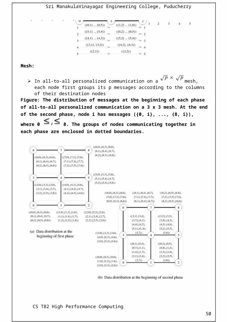
Sri ManakulaVinayagar Engineering College, Puducherry
sequential algorithm for solving the same problem on a single processing element. We denote the
overhead function of a parallel system by the symbol To.
5. Define speedup.
Speedup is a measure that captures the relative benefit of solving a problem in parallel. It is
defined as the ratio of the time taken to solve a problem on a single processing element to the time
required to solve the same problem on a parallel computer with p identical processing elements. We
denote speedup by the symbol S.
6. Define efficiency
Efficiency is a measure of the fraction of time for which a processing element is usefully
employed; it is defined as the ratio of speedup to the number of processing elements. In an ideal
parallel system, speedup is equal to p and efficiency is equal to one.
7. Define scalability of parallel system
The scalability of a parallel system is a measure of its capacity to increase speedup in
proportion to the number of processing elements. It reflects a parallel system's ability to utilize
increasing processing resources effectively.
8. The Isoefficiency Metric of Scalability (November 2013)
For a given problem size, as we increase the number of processing elements, the overall
efficiency of the parallel system goes down. This phenomenon is common to all parallel
systems.
In many cases, the efficiency of a parallel system increases if the problem size is increased
while keeping the number of processing elements constant.
9. What is degree of concurrency?
The maximum number of tasks that can be executed simultaneously at any time in a parallel
algorithm is called its degree of concurrency. The degree of concurrency is a measure of the number
of operations that an algorithm can perform in parallel for a problem of size W; it is independent of
the parallel architecture. If C(W) is the degree of concurrency of a parallel algorithm, then for a
problem of size W, no more than C(W) processing elements can be employed effectively.
10. What is the Key attributes that characterize the message-passing programming?
There are two key attributes that characterize the message-passing programming paradigm.
The first is that it assumes a partitioned address space and the second is that it supports only explicit
parallelization.
11. Write the basic operations in the message-passing programming.
The basic operations in the message-passing programming paradigm are send and receive. In their
simplest form, the prototypes of these operations are defined as follows:
send (void *sendbuf, intnelems, intdest)
CS T82 High Performance Computing 50

Sri ManakulaVinayagar Engineering College, Puducherry
receive (void *recvbuf, intnelems, int source)
12. Define Message-passing interface
The message-passing interface or MPI defines a standard library for message-passing that can
be used to develop portable message-passing programs using either C or FORTRAN. The MPI
standard defines both the syntax as well as the semantics of a core set of library routines that are very
useful in writing message-passing programs.
13. What is meant by Communication domain?
A key concept used throughout MPI is that of the communication domain. A communication
domain is a set of processes that are allowed to communicate with each other. Information about
communication domains is stored in variables of type MPI_Comm,that arecalled communicators.
14. Define communicator
The communicator is used to define a set of processes that can communicate with each other.
This set of processes form a communication domain. In general, all the processes may need to
communicate with each other. For this reason, MPI defines a default communicator called
MPI_COMM_WORLD which includes all the processes involved in the parallel execution.
15. Write the Basic functions for sending and receiving messages in MPI.
The basic functions for sending and receiving messages in MPI are the MPI_Send and
MPI_Recv, respectively. The calling sequences of these routines are as follows:
intMPI_Send(void *buf, int count, MPI_Datatypedatatype,
intdest, int tag, MPI_Commcomm)
intMPI_Recv(void *buf, int count, MPI_Datatypedatatype,
int source, int tag, MPI_Commcomm, MPI_Status *status)
16. Define Minimum Execution Time.(April 2013)
Minimum Execution Time is refers to increased execution time faster or minimum possible execution time of a parallel algorithm is, provided that the number of processing elements is not a constraint. As we increase the number of processing elements of a given problem size, either the parallel runtime continues to decease and asymptotically approaches a minimum value or it starts rising after attaining a minimum value.
17. What is synchronization primitive in Pthreads? (April 2013)
In communication is implicit in shared-address-space programming, much of the effort
associated with writing correct threaded programs is spent on synchronizing concurrent threads with
respect to their data accesses or scheduling.
CS T82 High Performance Computing 51
= 0

Sri ManakulaVinayagar Engineering College, Puducherry
Using pthread_createand pthread_join calls, we can create concurrent tasks. These tasks work together to manipulate data and accomplish a given task. When multiple threads attempt to manipulate the same data item, the results can often be incoherent if proper care is not taken to synchronize them. Consider the following code fragment being executed by multiple threads. The variable my_costis thread-local and best_costis a global variable shared by all threads.
1 /* each thread tries to update variable best_cost as follows */2 if (my_cost<best_cost)3 best_cost = my_cost;
11 MARKS
1. Elaborate on the various performance metrics used in studying the parallel systems.
(April 2013) (November 2013)
A number of metrics have been used based on the desired outcome of performance analysis.
Execution Time
The serial runtime of a program is the time elapsed between the beginning and the end of its
execution on a sequential computer.
The parallel runtime is the time that elapses from the moment a parallel computation starts to
the moment the last processing element finishes execution.
We denote the serial runtime by TS and the parallel runtime by TP.
Total Parallel Overhead
The overheads incurred by a parallel program are encapsulated into a single expression
referred to as the overhead function.
We define overhead function or total overhead of a parallel system as the total time
collectively spent by all the processing elements over and above that required by the fastest
known sequential algorithm for solving the same problem on a single processing element.
We denote the overhead function of a parallel system by the symbol To
The total time spent in solving a problem summed over all processing elements is pTP. TS
units of this time are spent performing useful work, and the remainder is overhead.
Therefore, the overhead function (To) is given by
Speedup
Speedup is a measure that captures the relative benefit of solving a problem in parallel.
CS T82 High Performance Computing 52

Sri ManakulaVinayagar Engineering College, Puducherry
It is defined as the ratio of the time taken to solve a problem on a single processing element to
the time required to solve the same problem on a parallel computer with p identical processing
elements.
We denote speedup by the symbol S.
Efficiency
Efficiency is a measure of the fraction of time for which a processing element is usefully
employed, it is defined as the ratio of speedup to the number of processing elements.
In an ideal parallel system, speedup is equal to p and efficiency is equal to one.
Otherwise, speedup is less than p and efficiency is between zero and one, depending on the
effectiveness with which the processing elements are utilized. We denote efficiency by the
symbol E.
Cost
We define the cost of solving a problem on a parallel system as the product of parallel runtime
and the number of processing elements used.
Cost reflects the sum of the time that each processing element spends solving the problem.
A parallel system is said to be cost-optimal if the cost of solving a problem on a parallel computer
has the same asymptotic growth (inQ terms) as a function of the input size as the fastest-known
sequential algorithm on a single processing element.
Cost is sometimes referred to as work or processor-time product, and a cost-optimal system is
also known as a pTP-optimal system.
CS T82 High Performance Computing 53

Sri ManakulaVinayagar Engineering College, Puducherry
Computing the globalsum of 16 partial sums using 16 processing elements . denotes the
sum of numbers with consecutive labels from i to j.
2. Explain any six MPI functions commonly used to perform collective communication
operations with an application (November 2013)
MPI defines a standard library for message-passing that can be used to develop portable message-passing programs using either C or FORTRAN.
The MPI standard defines both the syntax as well as the semantics of a core set of library routines.
Vendor implementations of MPI are available on almost all commercial parallel computers. It is possible to write fully-functional message-passing programs by using only the six
routines. These routines are used to initialize and terminate the MPI library, to get information about
the parallel computing environment, and to send and receive messages is shown in table.
Table 1: MPI Message Passing Interface
Starting and Terminating the MPI Library
MPI_Init is called prior to any calls to other MPI routines. Its purpose is to initialize the MPI environment.
MPI_Finalize is called at the end of the computation, and it performs various clean-up tasks to terminate the MPI environment.
The prototypes of these two functions are:intMPI_Init(int *argc, char ***argv)
intMPI_Finalize()
MPI_Init also strips off any MPI related command-line arguments. All MPI routines, data-types, and constants are prefixed by “MPI_”. The return code for
successful completion is MPI_SUCCESS. Communicators
A communicator defines a communication domain -a set of processes that are allowed to communicate with each other.
Information about communication domains is stored in variables of type MPI_Comm.
CS T82 High Performance Computing 54

Sri ManakulaVinayagar Engineering College, Puducherry
Communicators are used as arguments to all message transfer MPI routines. A process can belong to many different (possibly overlapping) communication domains. MPI defines a default communicator called MPI_COMM_WORLD which includes all the
processes Getting information The MPI_Comm_size and MPI_Comm_rank functions are used to determine the number of
processes and the label of the calling process, respectively. The calling sequences of these routines are as follows:
intMPI_Comm_size(MPI_Commcomm, int *size)
intMPI_Comm_rank(MPI_Commcomm, int *rank)
The function MPI_Comm_size returns in the variable size the number of processes that belong to the communicator comm.
So,MPI_Comm_size(MPI_COMM_WORLD, &size) will return in size the number of processors used by the program.
Every process that belongs to a communicator is uniquely identified by its rank. The rank of a process is an integer that ranges from zero up to the size of the communicator
minus one. A process can determine its rank in a communicator by using the MPI_Comm_rank function
that takes two arguments: the communicator and an integer variable rank. Up on return, the variable rank stores the rank of the process.
Example program:
#include <mpi.h>
main(intargc, char *argv[])
{
intnpes, myrank;
MPI_Init(&argc, &argv);
MPI_Comm_size(MPI_COMM_WORLD, &npes);
MPI_Comm_rank(MPI_COMM_WORLD, &myrank);
printf("From process %d out of %d, Hello World!\n",myrank, npes);
MPI_Finalize();
}
Sending and Receiving Messages
The basic functions for sending and receiving messages in MPI are the MPI_Send and MPI_Recv, respectively. The calling sequences of these routines are as follows:
intMPI_Send(void *buf, int count, MPI_Datatypedatatype,
intdest, int tag, MPI_Commcomm)
CS T82 High Performance Computing 55

Sri ManakulaVinayagar Engineering College, Puducherry
intMPI_Recv(void *buf, int count, MPI_Datatypedatatype,
int source, int tag, MPI_Commcomm, MPI_Status *status)
MPI_Send sends the data stored in the buffer pointed by buf. This buffer consists of consecutive entries of the type specified by the parameter datatype. The number of entries in the buffer is given by the parameter count.
However, MPI allows two additional datatypes that are not part of the C language. These are MPI_BYTE and MPI_PACKED.
MPI_BYTE corresponds to a byte (8 bits) and MPI_PACKED corresponds to a collection of data items that has been created by packing non-contiguous data.
MPI_Recv receives a message sent by a process whose rank is given by thesource in the communication domain specified by the comm argument. The tag of the sent message must be that specified by the tag argument. If there are many messages with identical tag from the same process, then any one of these messages is received.
MPI allows specification of wildcard arguments for both source and tag. If source is set to MPI_ANY_SOURCE, then any process of the communication domain can
be the source of the message. If tag is set to MPI_ANY_TAG, then messages with any tag are accepted. On the receive side, the message must be of length equal to or less than the length field
specified.
CS T82 High Performance Computing 56
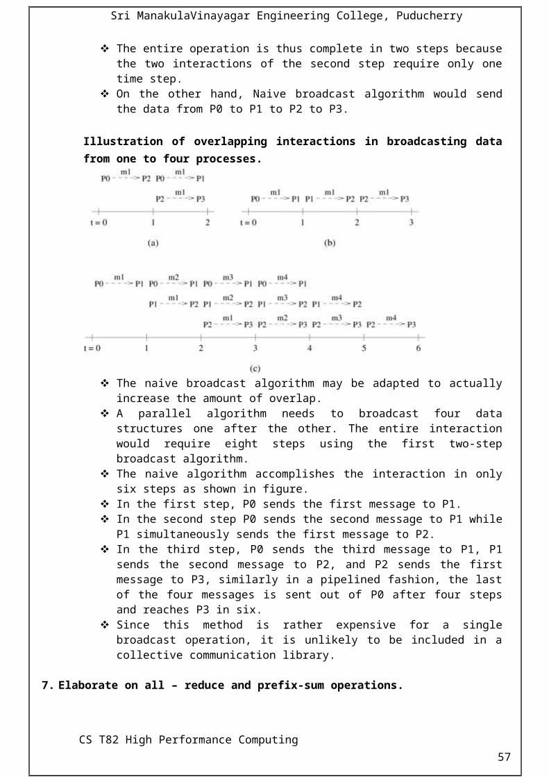
Sri ManakulaVinayagar Engineering College, Puducherry
On the receiving end, the status variable can be used to get information about the MPI_Recv operation.
The corresponding data structure contains:typedefstructMPI_Status
{
int MPI_SOURCE;
int MPI_TAG;
int MPI_ERROR;
};
The MPI_Get_count function returns the precise count of data items received.
intMPI_Get_count(MPI_Status *status, MPI_Datatypedatatype,int *count)
3. Explain collective communication and computation operations ( November 2013)
MPI provides an extensive set of functions for performing common collective communication operations.
Each of these operations is defined over a group corresponding to the communicator. All processors in a communicator must call these operations. The barrier synchronization operation is performed in MPI using:
intMPI_Barrier(MPI_Commcomm)
The one-to-all broadcast operation is:intMPI_Bcast(void *buf, int count, MPI_Datatypedatatype,int source,
MPI_Commcomm)
The all-to-one reduction operation is:
intMPI_Reduce(void *sendbuf, void *recvbuf, intcount,MPI_Datatypedatatype, MPI_Op op, inttarget,MPI_Commcomm)
Predefined Reduction Operation
CS T82 High Performance Computing 57

Sri ManakulaVinayagar Engineering College, Puducherry
The operation MPI_MAXLOC combines pairs of values (vi, li) and returns the pair (v, l) such that v is the maximum among all vi's and l is the corresponding li (if there are more than one, it is the smallest among all these li's).
MPI_MINLOC does the same, except for minimum value of vi.
An example use of the MPI _MINLOC and MPI _MAXLOC operators. MPI datatypes for data-pairs used with the MPI_ MAXLOC and MPI_MINLOC reduction
operations.
If the result of the reduction operation is needed by all processes, MPI provides:intMPI_Allreduce(void *sendbuf, void *recvbuf, intcount,MPI_Datatypedatatype, MPI_Op op, MPI_Commcomm)
To compute prefix-sums, MPI provides:intMPI_Scan(void *sendbuf, void *recvbuf, intcount,MPI_Datatypedatatype, MPI_Op op, MPI_Commcomm)
The gather operation is performed in MPI using:intMPI_Gather(void *sendbuf, intsendcount,MPI_Datatypesenddatatype, void *recvbuf, intrecvcount,MPI_Datatyperecvdatatype, int target, MPI_Commcomm)
MPI also provides the MPI_Allgather function in which the data are gathered at all the processes.
intMPI_Allgather(void *sendbuf, intsendcount,MPI_Datatypesenddatatype, void *recvbuf, intrecvcount,MPI_Datatyperecvdatatype, MPI_Commcomm)
The corresponding scatter operation is:intMPI_Scatter(void *sendbuf, intsendcount,MPI_Datatypesenddatatype, void *recvbuf, intrecvcount,MPI_Datatyperecvdatatype, int source, MPI_Commcomm)
The all-to-all personalized communication operation is performed by:intMPI_Alltoall(void *sendbuf, intsendcount,MPI_Datatypesenddatatype, void *recvbuf, intrecvcount,MPI_Datatyperecvdatatype, MPI_Commcomm)
Using this core set of collective operations, a number of programs can be greatly simplified.
CS T82 High Performance Computing 58

Sri ManakulaVinayagar Engineering College, Puducherry
4. Discuss minimum execution time and minimum cost optimal execution time (6 marks)
We are often interested in knowing how fast a problem can be solved, or what the minimum possible execution time of a parallel algorithm
We can determine the minimum parallel runtime for a given W by differentiating the expression for TP with respect to p and equating the derivative to zero (assuming that the function TP (W, p) is differentiable with respect to p).
Let be the minimum time in which a problem can be solved by a cost-optimal parallel system.
A problem of size W can be solved cost-optimally if and only if W = W (f(p)). In other words, given a problem of size W, a cost-optimal solution requires that p = O (f (W)).
Since the parallel runtime is Q(W/p) for a cost-optimal parallel system,the lower bound on the parallel runtime for solving a problem of size W cost-optimally is
From this equation:
We get,
5. Explain In Detail About Open Mp With Example?
Introduction:
Open Multi-Processing
The OpenMPAPIsupports multi-platform shared-memory parallel programming in C/C++ and Fortran.
The OpenMP API defines a portable, scalable model with a simple and flexible interface for developing parallel applications on platforms from the desktop to the supercomputer.
CS T82 High Performance Computing 59

Sri ManakulaVinayagar Engineering College, Puducherry
An illustration of multithreading where the master thread forks off a number of threads which execute blocks of code in parallel.
ARB:
The OpenMP Architecture Review Board (ARB) published its first API specifications, OpenMP for Fortran 1.0, in October 1997.
The OpenMP ARB (or just “ARB”) is the non-profit corporation that owns the OpenMP brand, oversees the OpenMP specification and produces and approves new versions of the specification.
Permanent Members of the ARB:
AMD ,CAPSEntreprise ,ConveyComputer ,Cray ,Fujitsu ,HP ,IBM ,Intel ,NEC ,NVIDIA ,Oracle Corporation ,Red Hat ,ST Microelectronics ,Texas Instruments.
Auxiliary Members of the ARB:
ANL ,ASC/LLNL ,BSC ,cOMPunity ,EPCC ,LANL ,NASA ,ORNL ,RWTHAachen University ,SNL-Sandia National Lab ,Texas Advanced Computing Center ,University of Houston.
RED HAT:
Red Hat has joined the OpenMP Architecture Review Board (ARB), a group of leading hardware and software vendors and research organizations creating the standard for today’s most prevalent shared-memory parallel programming model.
LIBDOUBANM:
This is a private library used to support a website.
libdoubanm is a data mining library, contains optimization and matrix/vector algorithms .OpenMP is used to parallelize the code.
With OpenMP, the threads number is reduced to one at each machine and the time/speed is improved greatly.
OpenMP is used to parallelize the matrix/vector operations automatically. OpenMP’s task is used for graph visit.
NAN-TOOLBOX:
A time series analysis, statistics and machine learning toolbox for Octave and Matlab® for data with and without MISSING VALUES encoded as NaN’s. (Statistics, Machine Learning, Signal processing)
The NaN-toolbox is about 30000 lines in total of both projects. The core functions using OpenMP contain aboout 1800 lines of C/C++ and Matlab/Octave and is available on Linux + Matlab/Octave,Win32/Win64 + Matlab, Debian/Ubuntu + Octave.
OpenMP API 4.0:
The OpenMP Consortium has released OpenMP API 4.0, a major upgrade of the OpenMP API standard language specifications.
CS T82 High Performance Computing 60

Sri ManakulaVinayagar Engineering College, Puducherry
New Features in the OPENMP 4.0 API Include:
Support for accelerators SIMD constructs to vectorize both serial as well as parallelized loops Error handling Thread affinity Tasking extensions Support for Fortran 2003 User-defined reductions Sequentially consistent atomics
Chart of OpenMP constructs:
Features of OpenMP Used:#pragma omp parallel#pragma omp for schedule(dynamic) nowait#pragma omp parallel for schedule(dynamic)
omp for or omp do:Used to split up loop iterations among the threads, also called loop constructs.The parallelization is done by the OpenMP directive #pragma omp.
Compilers:
OpenMP has been implemented in many commercial compilers. C/C++/FORTRAN,Visual C++ 2005, 2008 and 2010, gcc ,nagforas well as Intel Parallel Studio for various processors.
#include "stdafx.h"# include <cstdlib># include <iostream># include <iomanip># include <omp.h>
using namespace std;
int main ( int argc, char *argv[] );
//****************************************************************************80
CS T82 High Performance Computing 61

Sri ManakulaVinayagar Engineering College, Puducherry
int main ( int argc, char *argv[] )
//****************************************************************************80//// Purpose://// HELLO has each thread print out its ID.//// Discussion://// HELLO is a "Hello, World" program for OpenMP.//{ int id; double wtime;
cout << "\n"; cout << "HELLO_OPENMP\n"; cout << " C++/OpenMP version\n";
cout << "\n"; cout << " Number of processors available = " << omp_get_num_procs ( ) << "\n"; cout << " Number of threads = " << omp_get_max_threads ( ) << "\n";
wtime = omp_get_wtime ( );//// Have each thread say hello//# pragma omp parallel \ private ( id ) { id = omp_get_thread_num ( ); cout << " This is process " << id << "\n"; }//// Finish up by measuring the elapsed time.// wtime = omp_get_wtime ( ) - wtime;//// Terminate.// cout << "\n"; cout << "HELLO_OPENMP\n"; cout << " Normal end of execution.\n";
cout << "\n"; cout << " Elapsed wall clock time = " << wtime << "\n";
return 0;}
CS T82 High Performance Computing 62
Sri ManakulaVinayagar Engineering College, Puducherry
Output:
6. Explain Asymptotic Analysis of Parallel Programs and other scalability metrics.
Asymptotic Analysis of Parallel Programs:
Consider the problem of sorting a list of n numbers. The fastest serial programs for this problem run in timeO(n log n). Let us look at four different parallel algorithms A1, A2, A3, and A4, for sorting a given list. The parallel runtime of the four algorithms along with the number of processing elements they
can use is given in Table.
Table: Comparison of four different algorithms for sorting a given list of numbers. The table shows number of processing elements, parallel runtime, speedup, efficiency and the pTP product.
CS T82 High Performance Computing 63

Sri ManakulaVinayagar Engineering College, Puducherry
By this metric, algorithm A1 is the best, followed by A3, A4, and A2. This is also reflected in the fact that the speedups of the set of algorithms are also in this order.
Other Scalability Metrics
A number of other metrics of scalability of parallel systems have been proposed. These metrics are specifically suited to different system requirements
For example, in real time applications, the objective is to scale up a system to accomplish a task in a specified time bound.
One such application is multimedia decompression, where MPEG streams must be decompressed at the rate of 25 frames/second.A parallel system must decode a single frame in 40 ms (or with buffering, at an average of 1 frame in 40 ms over the buffered frames).Scaled Speedup
This metric is defined as the speedup obtained when the problem size is increased linearly with the number of processing elements.
If the scaled-speedup curve is close to linear with respect to the number of processing elements, then the parallel system is considered scalable.
In this case the scaled-speedup metric provides results very close to those of isoefficiency analysis, and the scaled-speedup is linear or near-linear with respect to the number of processing element
Two generalized notions of scaled speedup have been examinedo In one method, the size of the problem is increased to fill the available memory on the
parallel computer. The assumption here is that aggregate memory of the system increases with the number of processing elements. o In the other method, the size of the problem grows with p subject to an upper-bound on
execution time.
7. Discuss the building blocks of message passing.
The basic operations in the message-passing programming paradigm are send and receive. In their simplest form, the prototypes of these operations are defined as follows:
send(void *sendbuf, intnelems, intdest)
receive(void *recvbuf, intnelems, int source)
Consider the following code segments:
CS T82 High Performance Computing 64

Sri ManakulaVinayagar Engineering College, Puducherry
In this simple example, process P0 sends a message to process P1 which receives and prints the message. The process P0 changes the value of a to 0 immediately following the send.
The semantics of the send operation require that the value received by process P1 must be 100 as opposed to 0. That is, the value of a at the time of the send operation must be the value that is received by process P1.
This motivates the design of the send and receive protocols.
Blocking Message Passing OperationsThere are two mechanisms by which this can be achieved.
Blocking Non-Buffered Send/Receive The sending process sends a request to communicate to the receiving process. When the
receiving process encounters the target receives, it responds to the request. The sending process upon receiving this response initiates a transfer operation.Since there are no buffers used at either sending or receiving ends, this is also referred to as a non-buffered blocking operation
Idling Overheads in Blocking Non-Buffered Operations, we will discuss three scenarios in which the send is reached before the receive is posted, the send and receive are posted around the same time, and the receive is posted before the send is reached.
In cases (a) and (c), we notice that there is considerable idling at the sending and receiving process.
Figure: Handshake for a blocking non-buffered send/receive operation. It is easy to see that
in cases where sender and receiver do not reach communication point at similar times, there can be considerable idling overheads.
Blocking Buffered Send/Receive A simple solution to the idling and deadlocking problem outlined above is to rely on buffers at
the sending and receiving ends. The sender simply copies the data into the designated buffer and returns after the copy
operation has been completed. The data must be buffered at the receiving end as well. Buffering trades off idling overhead for buffer copying overhead. Figure: Blocking buffered transfer protocols: (a) in the presence of communication
hardware with buffers at send and receive ends; and (b) in the absence of
CS T82 High Performance Computing 65

Sri ManakulaVinayagar Engineering College, Puducherry
communication hardware, sender interrupts receiver and deposits data in buffer at receiver end.
Deadlocks in Buffered Send and Receive Operations While buffering alleviates many of the deadlock situations, it is still possible to write code
that deadlocks. This is due to the fact that as in the non-buffered case, receive calls are always blocking (to
ensure semantic consistency). Thus, a simple code fragment such as the following deadlocks since both processes wait to
receive data but nobody sends it.
Once again, such circular waits have to be broken. However, deadlocks are caused only by waits on receive operations in this case.
Non-Blocking Message Passing Operations The programmer must ensure semantics of the send and receive. This class of non-blocking protocols returns from the send or receive operation before it is
semantically safe to do so. Non-blocking operations are generally accompanied by a check-status operation. When used correctly, these primitives are capable of overlapping communication overheads
with useful computations. Message passing libraries typically provide both blocking and non-blocking primitives.
CS T82 High Performance Computing 66

Sri ManakulaVinayagar Engineering College, Puducherry
Figure 1: Non-blocking non-buffered send and receive operations (a) in absence of communication hardware; (b) in presence of communication hardware.
Non-blocking operations can themselves be buffered or non-buffered. In the non-buffered case, a process wishing to send data to another simply posts a pending message and returns to the user program.This is shown in figure 2.
Figure 2: Space of possible protocols for send and receive operations.
8. Explain in detail about shared address space platforms.
Here, we discuss shared-address-space programming paradigms along with their performance issues and related extensions to directive-based paradigms.
Shared address space programming paradigms can vary on mechanisms for data sharing, concurrency models, and support for synchronization.
Thread Basics
A thread is a single stream of control in the flow of a program.
CS T82 High Performance Computing 67

Sri ManakulaVinayagar Engineering College, Puducherry
for (row = 0; row < n; row++)
for (column = 0; column < n; column++)
c[row][column] =dot_product(get_row(a, row),get_col(b, col));
can be transformed to:
for (row = 0; row < n; row++)
for (column = 0; column < n; column++)
c[row][column] =create_thread(dot_product(get_row(a, row),get_col(b, col)));
In this case, one may think of the thread as an instance of a function that returns before the function has finished executing.
All memory in the logicalmachine model of a thread is globally accessible to every thread. The stack corresponding to the function call is generally treated as being local to the thread for
liveness reasons. This implies a logical machine model with both global memory (default) and local memory
(stacks). It is important to note that such a flat model may result in very poor performance since
memory is physically distributed in typical machines.
The logical machine model of a thread-based programming paradigm.
Why Threads?
Threaded programming models offer significant advantages over message-passing programming models along with some disadvantages as well, let us briefly look at some of these.
Threads provide software portability. Inherent support for latency hiding. Scheduling and load balancing. Ease of programming and widespread use.
CS T82 High Performance Computing 68

Sri ManakulaVinayagar Engineering College, Puducherry
Software Portability Threaded applications can be developed on serial machines and run on parallel machines without any changes.This ability to migrate programs between diverse architectural platforms is a very significant advantage of threaded APIs.
Latency Hiding One of the major overheads in programs (both serial and parallel) is the access latency for memory access, I/O, and communication. By allowing multiple threads to execute on the same processor, threaded APIs enable this latency to be hidden
Scheduling and load balancing: Threaded APIs allow the programmer to specify a large number of concurrent tasks and support system-level dynamic mapping of tasks to processors with a view to minimizing idling overheads. By providing this support at the system level, threaded APIs rid the programmer of the burden of explicit scheduling and load balancing.
Easeof programming and widespread use: With widespread acceptance of the POSIX thread API, development tools for POSIX threads are more widely available and stable. These issues are important from the program development and software engineering aspects.
The POSIX Thread API Commonly referred to as Pthreads, POSIX has emerged as the standard threads API,
supported by most vendors. The concepts discussed here are largely independent of the API and can be used for
programming with other thread APIs (NT threads, Solaris threads, Java threads, etc.) as well.Thread Basics: Creation and Termination
Let us start with a simple threaded program for computing the value of p.
Pthreads provides two basic functions for specifying concurrency in a program:#include <pthread.h>
intpthread_create (pthread_t *thread_handle,constpthread_attr_t *attribute,void * (*thread_function)(void *),void *arg);
intpthread_join (pthread_tthread,void **ptr);
The function pthread_create invokes function thread_function as a thread. The pthread_create function creates a single thread that corresponds to the invocation of the
function thread_function (and any other functions called by thread_function). On successful creation of a thread, a unique identifier is associated with the thread and
assigned to the location pointed to by thread_handle. The thread has the attributes described by the attribute argument. The arg field specifies a pointer to the argument to function thread_function. This argument is
typically used to pass the workspace and other thread-specific data to a thread. The main program must wait for the threads to run to completion.This is done using the
function pthread_join which suspends execution of the calling thread until the specified thread terminates. The prototype of the pthread_join function is as follows:1) int
2) pthread_join (
3) pthread_t thread,
4) void **ptr);
CS T82 High Performance Computing 69

Sri ManakulaVinayagar Engineering College, Puducherry
A call to this function waits for the termination of the thread whose id is given by thread. On a successful call to pthread_join, the value passed to pthread_exit is returned in the
location pointed to by ptr. On successful completion, pthread_join returns 0, else it returns an error-code.
Synchronization Primitives in Pthreads
When multiple threads attempt to manipulate the same data item, the results can often be incoherent if proper care is not taken to synchronize them.
Consider:
/* each thread tries to update variable best_cost as follows */
if (my_cost<best_cost)
best_cost = my_cost;
Assume that there are two threads, the initial value of best cost is 100, and the values of my cost are 50 and 75 at threads t1 and t2.
Depending on the schedule of the threads, the value of best cost could be 50 or 75. The value 75 does not correspond to any serialization of the threads.
Mutual Exclusion: The code in the previous example corresponds to a critical segment; i.e., a segment that must
be executed by only one thread at any time. Critical segments in Pthreads are implemented using mutex locks. Mutex-locks have two states: locked and unlocked. At any point of time, only one thread can
lock a mutex lock. A lock is an atomic operation. A thread entering a critical segment first tries to get a lock. It goes ahead when the lock is
granted. The Pthreads API provides the following functions for handling mutex-locks:
intpthread_mutex_lock (pthread_mutex_t *mutex_lock);
intpthread_mutex_unlock (pthread_mutex_t *mutex_lock);
Example:Producer-Consumer Using Locks
The producer-consumer scenario imposes the following constraints:
The producer threadmust not overwrite the shared buffer when the previous task has not been picked up by a consumer thread.
The consumer threads must not pick up tasks until there is something present in the shared data structure.
Individual consumer threads should pick up tasks one at a time.Types of Mutexes
Pthreads supports three types of mutexes: normal, recursive, and error-check.
A normal mutex deadlocks if a thread that already has a lock tries a second lock on it. A recursive mutex allows a single thread to lock a mutex as many times as it wants. It simply
increments a count on the number of locks. A lock is relinquished by a thread when the count becomes zero.
CS T82 High Performance Computing 70
Sri ManakulaVinayagar Engineering College, Puducherry
An error check mutex reports an error when a thread with a lock tries to lock it again (as opposed to deadlocking in the first case, or granting the lock, as in the second case).
The type of the mutex can be set in the attributes object before it is passed at time of initialization.
Condition Variables for Synchronization
A condition variable is a data object used for synchronizing threads. This variable allows a thread to block itself until specified data reaches a predefined state.
A condition variable is associated with this predicate. When the predicate becomes true, the condition variable is used to signal one or more threads waiting on the condition.
A single condition variable may be associated with more than one predicate. A condition variable always has a mutex associated with it. A thread locks this mutex and
tests the predicate defined on the shared variable. If the predicate is not true, the thread waits on the condition variable associated with the
predicate using the function pthreadcond wait.
Pthreads provides the following functions for condition variables:intpthread_cond_wait(pthread_cond_t *cond,pthread_mutex_t *mutex);
intpthread_cond_signal(pthread_cond_t *cond);
intpthread_cond_broadcast(pthread_cond_t *cond);
Controlling Thread and Synchronization Attributes The Pthreads API allows a programmer to change the default attributes of entities using
attributes objects. An attributes object is a data-structure that describes entity(thread, mutex, condition variable)
properties. Once these properties are set, the attributes object can be passed to the method initializing the
entity. Enhances modularity, readability, and ease of modification.
Attributes Objects for Threads
Use pthread _attr _init to create an attributes object. Individual properties associated with the attributes object can be changed using the following
functions:pthread _attr _setdetachstate,
pthread _attr _setguardsize_ np,
pthread _attr _setstacksize,
pthread _attr _setinheritsched,
pthread _attr _setschedpolicy, and pthreadattrsetschedparam.
Attributes Objects for Mutexes
Initialize the attrributes object using function: pthread _mutexattr_init.
CS T82 High Performance Computing 71

Sri ManakulaVinayagar Engineering College, Puducherry
The function pthreadmutexattr_settype _np can be used for setting the type of mutex specified by the mutex attributes object.
pthread_mutexattr_settype_np (pthread_mutexattr_t *attr,int type);
Here, type specifies the type of the mutex and can take one of: PTHREAD_MUTEX _NORMAL _NP PTHREAD _MUTEX_ RECURSIVE _NP PTHREAD _MUTEX _ERRORCHECK_ NP
Thread Cancellation
A thread may cancel itself or cancel other threads. When a call to this function is made, a cancellation is sent to the specified thread.
Threads can protect themselves against cancellation. When a cancellation is actually performed, cleanup functions are invoked for reclaiming the thread data structures.
This process is similar to termination of a thread using the pthread_exit call. Posix threads provide this cancellation feature in the function pthread_cancel. The prototype
of this function is:1 int
2 pthread_cancel (
3 pthread_t thread);
Composite Synchronization Constructs
By design, Pthreads provide support for a basic set of operations. Higher level constructs can be built using basic synchronization constructs. We discuss two such constructs: read-write locks and barriers
Read-Write Locks
In many applications, a data structure is read frequently but written infrequently. For such applications, we should use read-write locks.
A read lock is granted when there are other threads that may already have read locks. If there is a write lock on the data (or if there are queued write locks), the thread performs a
condition wait. If there are multiple threads requesting a write lock, they must perform a condition wait. With this description, we can design functions for read locks mylib _rwlock_ rlock, write
locks mylib_ rwlock _wlock, and unlocking mylib _rwlock _unlock. The function mylib _rwlock_ rlock attempts a read lock on the data structure. It checks to see
if there is a write lock or pending writers. If so, it performs a condition wait on the condition variable readers proceed.
The function mylib_rwlock_wlock attempts a write lock on the data structure. It checks to see if there are readers or writers; if so, it increments the count of pending writers and performs a condition wait on the condition variable writer_proceed.
The function mylib_rwlock_unlock unlocks a read or write lock.Barriers
A barrier holds a thread until all threads participating in the barrier have reached it. Barriers can be implemented using a counter, a mutex and a condition variable.
CS T82 High Performance Computing 72

Sri ManakulaVinayagar Engineering College, Puducherry
A single integer is used to keep track of the number of threads that have reached the barrier. If the count is less than the total number of threads, the threads execute a condition wait. The last thread entering (and setting the count to the number of threads) wakes up all the
threads using a condition broadcast.
Barrier program:
typedefstruct {
pthread_mutex_tcount_lock;
pthread_cond_tok_to_proceed;
int count;
} mylib_barrier_t;
voidmylib_init_barrier(mylib_barrier_t *b) {
b -> count = 0;
pthread_mutex_init(&(b ->count_lock), NULL);
pthread_cond_init(&(b ->ok_to_proceed), NULL);
}
voidmylib_barrier (mylib_barrier_t *b, intnum_threads) {
pthread_mutex_lock(&(b ->count_lock));
b -> count ++;
if (b -> count == num_threads) {
b -> count = 0;
pthread_cond_broadcast(&(b ->ok_to_proceed));
}
Else
while (pthread_cond_wait(&(b ->ok_to_proceed),
&(b ->count_lock)) != 0);
pthread_mutex_unlock(&(b ->count_lock));
}
The barrier described above is called a linear barrier. The trivial lower bound on execution time of this function is therefore O(n) for n threads. This implementation of a barrier can be speeded up using multiple barrier variables organized
in a tree.
CS T82 High Performance Computing 73

Sri ManakulaVinayagar Engineering College, Puducherry
This process repeats up the tree.This is also called a log barrier and its runtime grows as O(log p).
UNIT – III
QUESTION BANK
2 MARKS
1. Define Inter-process Interaction 2. What is the Performance Metrics for Parallel Systems?3. Define Execution time?4. Define Total Parallel Overhead.5. Define speedup.6. Define efficiency7. Define scalability of parallel system8. The Isoefficiency Metric of Scalability (November 2013)9. What is degree of concurrency?10. What is the Key attributes that characterize the message-passing programming?11. Write the basic operations in the message-passing programming.12. Define Message-passing interface13. What is meant by Communication domain?14. 14.Define communicator15. Write the Basic functions for sending and receiving messages in MPI.16. Define Minimum Execution Time. (April 2013)17. What is synchronization primitive in Pthreads? (April 2013)
11 MARKS
1. Elaborate on the various performance metrics used in studying the parallel systems. 2. (April 2013) (November 2013)(Ref.Pg.No.51)3. Explain any six MPI functions commonly used to perform collective communication
operations with an application (November 2013) (Ref.Pg.No.53)4. Explain collective communication and computation operations ( November 2013)
(Ref.Pg.No.57)5. Discuss minimum execution time and minimum cost optimal execution time (6 marks)6. Explain in detail about open mp with example?7. Explain Asymptotic Analysis of Parallel Programs and other scalability metrics.8. Discuss the building blocks of message passing.9. Explain in detail about shared address space platforms.
CS T82 High Performance Computing 74

Sri ManakulaVinayagar Engineering College, Puducherry
UNIT – IV
Dense Matrix Algorithms:
Matrix-vector multiplication
Matrix-matrix multiplication
Solving a system of linear equations
FFT.
Sorting:
Issues in sorting on parallel computers
Sorting networks
Bubble sort and its variants
Quicksort
Bucket and sample sort
Other sorting algorithms.
Graph Algorithms:
Definitions and representation
Minimum spanning tree
Single-source shortest paths
All-pairs shortest paths.
TWO MARKS
1. What is a dense matrix algorithm?
Algorithms involving matrices and vectors are applied in several numerical and non numerical
contexts. Some key algorithm for dense algorithm.
1. Define Bitonic Sequence. (November 2013)
One of the key aspects of the bitonic algorithm is that it is communication intensive, and a
proper mapping of the algorithm must take into account the topology of the underlying
interconnection network.
The bitonic sorting network for sorting n elements contains log n stages, and stage i consists
of i columns of n/2 comparators.
3. Write Matrix vector multiplication algorithm.
procedure MAT-VECT(A,X,Y)
begin
for i=0to n-1 do
begin
CS T82 High Performance Computing 75

Sri ManakulaVinayagar Engineering College, Puducherry
y[i]:=0;
for j:=0 to n-1 do
y[i]:=y[i]+A[i,j]*x[j];
end for;
end MAT-VECT
3. What is block matrices operations?
It express a matrix computation involving scalar algebraic operations on all its elements in
terms of identical matrix algebraic operations on blocks or sub matrices of the original matrix.uch
algebraic operations on the sub matrices are called block matrix operations.
4. What is DNS algorithm?
It based on partitioning intermediate data that can use up to n3 processes and that performs
matrix multiplication in time (n3/log n) processes. This algorithm is known as the DNS algorithm.
5. What is LU Factorization?
In the context of upper-triangularization, a similar procedure can be used to factorize matrix A
as the product of a lower-triangular matrix L and a unit upper- triangular matrix U so that
A=L*U .This factorization is commonly referred to as LU factorization.
6. What is pipelined Gaussian elimination?
The performance of the algorithm can be improved substantially if the processes work
asynchronously; that is, no process waits for the others to finish an iteration before the starting the
next one. We call this the asynchronous or pipelined version of Gaussian elimination
7. What is partial pivoting?
The Gaussian elimination algorithm in algorithm fails if any diagonal entry A [K, K] of the
matrix of coefficients is close o equal to zero. To avoid this problem and to ensure the numerical
stability of the algorithm, a technique called partial pivoting.
8. What is scaled speedup?
It is defined as the problem size is increased linearly with the number of processes; that is if
W is chosen as a base problem size for a single process. Then
Scaled speedup=wp/Tp(Wp-p)
9. What is sorting?
It is defined as the task of arranging n unordered collection of elements into monotonically
increasing (or decreasing) order.
10. Types of sorting?
They are 2 types of sorting are
1. Internal sorting
2. External sorting
CS T82 High Performance Computing 76

Sri ManakulaVinayagar Engineering College, Puducherry
11. What is internal sorting?
The number of elements to be sorted is small enough to fit into the process main memory. It is
also called as internal sorting.
12. What is external sorting?
It uses auxiliary storage (such as tapes and hard disks) for sorting because the number of
elements to be sorted is too large to fit into memory. It is also called as external sorting.
13. What is comparison based algorithm?
It is unordered sequence of elements by repeatedly comparing pairs of elements and, if they
are out of order, exchanging them. This fundamental operation of comparison based sorting is called
compare exchange.
14. What is comparator?
It is a device with two inputs x and y and two output x’ and y’. It is also called as comparator.
15. Types of comparator?
2types are
1. Increasing comparator
2. Decreasing comparator
16. What is Bitonic sort? (November 2013)
A bitonic sorting network sorts n elements in (log2 n) time. The key operation of the bitonic
sorting network is the rearrangement of a bitonic sequence into a sorted sequence.
17. What is shell sort?
It is one such serial sorting algorithm. Let n be the number of elements to be sorted and p be
the number of processes. Each process is assigned a block of n/p elements.
18. What is quick sort?
Quick sort is a divide conquer algorithm that’s sorts a sequence by recursively dividing it into
smaller sub sequences.
19. What is bucket sort?
It sorting an array of n elements whose values are uniformly distributed over an interval [a, b]
is the bucket sort. It is also called bucket sort
20. What is sample sort?
The bucket sort may result in buckets that have a significantly different number of elements,
degrading performance. In such situation an algorithm called sample sort.
21. What is spanning tree?
It is undirected graph G is a sub graph of G that is a tree containing all the vertices of G. It is
also known as spanning tree.
CS T82 High Performance Computing 77
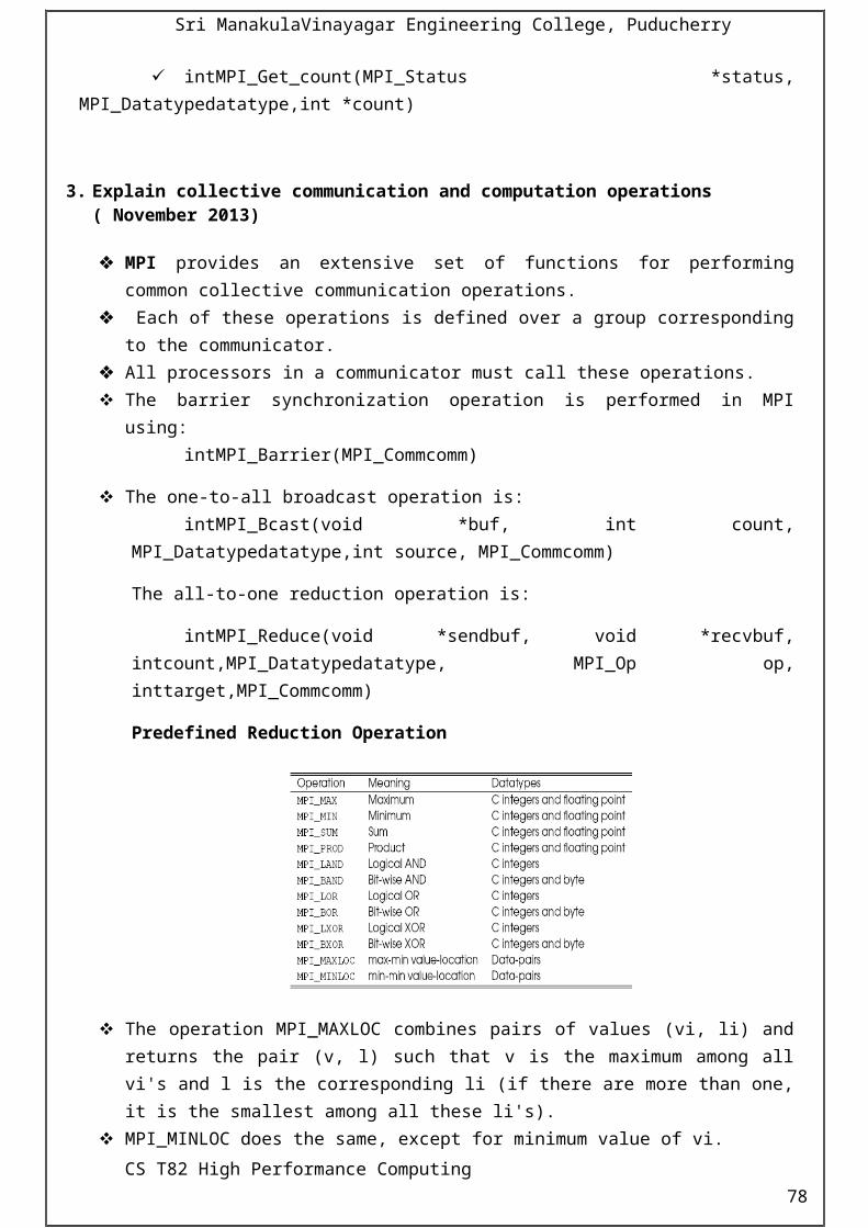
Sri ManakulaVinayagar Engineering College, Puducherry
22. What is weighted graph?
The weight of a sub graph is the sum of the weight of the edges in the sub graph .It is also
known weighted graph.
23. What is minimum spanning tree? (April 2013)
It denote as MST. The minimum spanning tree for a weighted undirected graph is a spanning
tree with minimum weight.
24. What is shortest path?
It is minimum weight path. it depend on the application, edge, weights may represent time ,
cost, penalty, loss or any other quantity that accumulates additively along a path and is to be
minimized.
25. What is connected components?
The connected components of an undirected graph are the equivalence classes of vertices
under the “is reachable from “relation.
26. Define sorting networks (April 2013)
Sorting networks are based on a comparison network model, in which many comparison
operations are performed simultaneously.
The key component of these networks is a comparator. A comparator is a device with two
inputsx and y and two outputs x' and y'. For an increasing comparator, x' = min{x, y} and y' =
max{x, y}; for a decreasing comparator x' = max{x, y} and y' = min{x, y}.
A sorting network is usually made up of a series of columns, and each column contains a
number of comparators connected in parallel.
11 MARKS
1. Explain how the parallel implementation of Gaussian elimination algorithm is used in solving a system of linear equations. (November 2013)
The problem of solving a system of linear equations of the form is discussed here:
In matrix notation, this system is written as Ax = b. A system of equations Ax = b is usually solved in two stages. First, through a series of
algebraic manipulations, the original system of equations is reduced to an upper-triangular system of the form
CS T82 High Performance Computing 78

Sri ManakulaVinayagar Engineering College, Puducherry
We write this as Ux= y, where U is a unit upper-triangular matrix – one in which all subdiagonal entries are zero and all principal diagonal entries are equal to one.
A Simple Gaussian Elimination Algorithm
The serial Gaussian elimination algorithm has three nested loops. Several variations of the algorithm exist, depending on the order in which the loops are arranged.
Algorithm: A serial Gaussian elimination algorithm that converts the system of linear
equationsAx = b to a unit upper-triangular system Ux= y. The matrix U occupies the
upper-triangular locations of A. This algorithm assumes that A[k, k] 0 when it is used as a divisor on lines 6 and 7.
1. procedureGAUSSIAN_ELIMINATION (A, b, y)
2. begin
3. for k := 0 to n - 1 do /* Outer loop */
4. begin
5. for j :=k + 1 to n - 1 do
6. A[k, j] := A[k, j]/A[k, k]; /* Division step */
7. y[k] := b[k]/A[k, k];
8. A[k, k] := 1;
9. for i :=k + 1 to n - 1 do
10. begin
11. for j :=k + 1 to n - 1 do
12. A[i, j] := A[i, j] - A[i, k] x A[k, j]; /* Elimination step */
13. b[i] := b[i] - A[i, k] x y[k];
14. A[i, k] := 0;
15. endfor; /* Line 9 */
16. endfor; /* Line 3 */
CS T82 High Performance Computing 79

Sri ManakulaVinayagar Engineering College, Puducherry
17. endGAUSSIAN_ELIMINATION
Gaussian Elimination with Partial Pivoting
The Gaussian elimination algorithm in Algorithm 8.4 fails if any diagonal entry A[k, k] of the matrix of coefficients is close or equal to zero.
To avoid this problem and to ensure the numerical stability of the algorithm, a technique called partial pivoting is used.
At the beginning of the outer loop in the kth iteration, this method selects a column i (called the pivot column) such that A[k, i] is the largest in magnitude among all A[k, j] such that k
j <n. It then exchanges the kth and the i th columns before starting the iteration. These columns can either be exchanged explicitly by physically moving them into each other's
locations, or they can be exchanged implicitly by simply maintaining an n x 1 permutation vector to keep track of the new indices of the columns of A.
2. Explain in detail Matrix vector multiplication. (April 2013)
The problem of multiplying a dense n x n matrix A with an n x 1 vector x to yield the n x 1 result vector y.
The Algorithm shows a serial algorithm for this problem. The sequential algorithm requires n2 multiplications and additions.
Assuming that a multiplication and addition pair takes unit time, the sequential run time is
At least three distinct parallel formulations of matrix-vector multiplication are possible, depending on whether
o rowwise 1-Do columnwise 1-Do 2-D partitioning is used.
Algorithm :A serial algorithm for multiplying an n x n matrix A with an n x 1 vector x to yield an n x 1 product vector y.
1. procedureMAT_VECT ( A, x, y)
2. begin
3. for i := 0 to n - 1 do
4. begin
5. y[i]:=0;
6. for j := 0 to n - 1 do
7. y[i] := y[i] + A[i, j] x x[j];
8. endfor;
9. endMAT_VECT
CS T82 High Performance Computing 80

Sri ManakulaVinayagar Engineering College, Puducherry
Row-wise 1-D Partitioning
The parallel algorithm for matrix-vector multiplication using rowwise block 1-D partitioning is discussed.
Figure 1: describes the distribution and movement of data for matrix-vector multiplication with block 1-D partitioning.
Multiplication of an n x n matrix with an n x 1 vector using rowwise block 1-D partitioning. For the one-row-per-process case, p = n.
One Row per Process
First, consider the case in which the n x n matrix is partitioned among n processes so that each process stores one complete row of the matrix.
The n x 1 vector x is distributed such that each process owns one of its elements. The initial distribution of the matrix and the vector for rowwise block 1-D partitioning is
shown in Figure (a). Since each process starts with only one element of x, an all-to-all broadcast is required to
distribute all the elements to all the processes in figure(b) After the vector x is distributed among the processes in figure(c) The result vector y is stored exactly the way the starting vector x was stored is shown in
figure(d). Thus, the entire procedure is completed by n processes in time Q (n), resulting in a process-
time product of Q (n2). The parallel algorithm iscost-optimal because the complexity of the serial algorithm is Q (n2).
Using Fewer than n Processes
Consider the case in which p processes are used such that p <n, and the matrix is partitioned among the processes by using block 1-D partitioning.
CS T82 High Performance Computing 81

Sri ManakulaVinayagar Engineering College, Puducherry
Each process initially stores n/p complete rows of the matrix and a portion of the vector of size n/p. Since the vector x must be multiplied with each row of the matrix, every process needs the entire vector.
This again requires an all-to-all broadcast as shown in Figure (b) and (c).
2-D PartitioningThis section discusses parallel matrix-vector multiplication for the case in which the matrix is distributed among the processes using a block 2-D partitioning.
Matrix-vector multiplication with block 2-D partitioning. For the one-element-per-process case, p = n2 if the matrix size is n x n.
One Element Per Process
As Figure (a) shows, the first communication step for the 2-D partitioning aligns the vector x along the principal diagonal of the matrix.
The second step copies the vector elements from each diagonal process to all the processes in the corresponding column is shown in figure (b).
Figure (c) shows this step, which requires an all-to-one reduction in each row with the last process of the row as the destination.
The parallel matrix-vector multiplication is complete after the reduction step. The overall parallel run time of this algorithm is Q (n). The cost (process-time product) is Q (n2 log n). Hence, the algorithm is not cost-optimal.
Using Fewer than n2 Processes
A cost-optimal parallel implementation of matrix-vector multiplication with block 2-D partitioning of the matrix can be obtained, if the granularity of computation at each process is increased by using fewer than n2 processes.
CS T82 High Performance Computing 82

Sri ManakulaVinayagar Engineering College, Puducherry
The initial data-mapping and the various communication steps for this case is shown in figure (a).
The entire vector must be distributed on each row of processes before the multiplication can be performed. First, the vector is aligned along the main diagonal.
Then a columnwise one-to-all broadcast of these elements takes place. Each process
then performs n2/p multiplications and locally adds the sets of products. At the end of this step in figure(c), each process has partial sums that must be accumulated
along each row to obtain the result vector. Hence, the last step of the algorithm is an all-to-one reduction of the values in each row, with
the rightmost process of the row as the destination. Thus, the parallel run time for this procedure is as follows:
Comparison of 1-D and 2-D Partitionings
If the number of processes is greater than n, then the 1-D partitioning cannot be used. However, even if the number of processes is less than or equal to n, the analysis in this section suggests that 2-D partitioning is preferable.
Among the two partitioning schemes, 2-D partitioning has a better (smaller) asymptotic isoefficiency function.
Thus, matrix-vector multiplication is more scalable with 2-D partitioning, i.e it can deliver the same efficiency on more processes with 2-D partitioning than with 1-D partitioning.
3. Discuss in cannon’s and DNS algorithm in details.
Cannon's Algorithm
Cannon's algorithm is a memory-efficient version of the simple algorithm To study this algorithm, we again partition matrices A and B into p square blocks. The first communication step of the algorithm aligns the blocks of A and B in such a way that
each process multiplies its local submatrices, this alignment is achieved for matrix A by shifting all submatrices Ai, j to the left (with wraparound) by i steps in figure(a).
Similarly, all submatrices Bi, j are shifted up (with wraparound) by j steps. These are circular shift operations in Figure(b)
Figure 8.3(c) shows the blocks of A and B after the initial alignment, when each process is ready for the first submatrix multiplication. After a submatrix multiplication step, each block of A moves one step left and each block of B moves one step up (again with wraparound)as shown in Figure (d).
A sequence of such submatrix multiplications and single-step shifts pairs up each Ai, k and Bk, j for at Pi, j. This completes the multiplication of matrices A and B.Figure: The communication steps in Cannon's algorithm on 16 processes.
CS T82 High Performance Computing 83

Sri ManakulaVinayagar Engineering College, Puducherry
Thus, the approximate overall parallel run time of this algorithm is
CS T82 High Performance Computing 84

Sri ManakulaVinayagar Engineering College, Puducherry
The DNS Algorithm
The matrix multiplication algorithms presented so far use block 2-D partitioning of the input and the output matrices and use a maximum of n2processes for n x n matrices.
As a result, these algorithms have a parallel run time of W (n) because there are Q (n3) operations in the serial algorithm.
We now present a parallel algorithm based on partitioning intermediate data that can use upton3processes and that performs matrix multiplication in time Q(log n) by using W(n3/log n) processes.
This algorithm is known as the DNS algorithm because it is due to Dekel, Nassimi, and Sahni. Figure: The communication steps in the DNS algorithm while multiplying 4 x 4 matrices
A and B on 64 processes. The shaded processes in part (c) store elements of the first row of A and the shaded processes in part (d) store elements of the first column of B.
The DNS algorithm has three main communication steps: (1) Moving the columns of A and the rows of B to their respective planes
(2) Performing one-to-all broadcast along the j axis for A and along the i axis for B
3) All-to-one reduction along the k axis. All these operations are performed within groups of n processes and take time Q (log n).
CS T82 High Performance Computing 85

Sri ManakulaVinayagar Engineering College, Puducherry
Thus, the parallel run time for multiplying two n x n matrices using the DNS algorithm on n3 processes is Q (log n).
Assume that the number of processes p is equal to q3for some q <n. To implement the DNS algorithm, the two matrices are partitioned into blocks of size (n/q) x
(n/q). Each matrix can thus be regarded as a q x q two-dimensional square array of blocks. The implementation of this algorithm on q3processes is very similar to that on n3processes. We get the following approximate expression for the parallel run time of the DNS algorithm:
4. Explain in detail about quick sort in parallel ( April 2013)
Quick sort is one of the most common sorting algorithms for sequential computers because of its simplicity, low overhead and optimal average complexity.
Quick sort is a divide-and-conquer algorithm that sorts a sequence by recursively dividing it into smaller subsequences. Assume that the n-element sequence to be sorted is stored in the array A[1...n]. Quick sort consists of two steps: divide and conquer.
During the divide step, a sequence A[q...r] is partitioned (rearranged) into two nonempty subsequences A[q...s] and A[s + 1...r] such that each element of the first subsequence is smaller than or equal to each element of the second subsequence.
During the conquer step, the subsequences are sorted by recursively applying quick sort. Since the subsequences A[q...s] and A[s + 1...r] are sorted and the first subsequence has smaller elements than the second, the entire sequence is sorted.
The sequence A[q...r] partitioned into two parts – one with all elements smaller than the other. This is usually accomplished by selecting one element x from A[q...r] and using this element
to partition the sequence A[q...r] into two parts – one with elements less than or equal to x and the other with elements greater than x. Element x is called the pivot.
Figure: Example of the quick sort algorithm sorting a sequence of size n= 8.
Algorithm: The sequential quicksort algorithm.
1. procedureQUICKSORT (A, q, r)
2. begin
3. ifq <r then
4. begin
CS T82 High Performance Computing 86

Sri ManakulaVinayagar Engineering College, Puducherry
5. x:= A[q];
6. s:= q;
7. for i :=q + 1 to r do
8. ifA[i] x then
9. begin
10. s:= s + 1;
11. swap(A[s], A[i]);
12. end if
13. swap(A[q], A[s]);
14. QUICKSORT (A, q, s);
15. QUICKSORT (A, s + 1, r);
16. end if
17. endQUICKSORT
Although quicksort can have O (n2) worst-case complexity, its average complexity is significantly better.
Parallelizing Quicksort
Quicksort can be parallelized in a variety of ways We present three distinct parallel formulations:
o One for a CRCW PRAM, o One for a shared-address-space architectureo One for a message-passing platform.
Each of these formulations parallelizes quicksort by performing the partitioning step in parallel.
1. Parallel Formulation for a CRCW PRAM
An arbitrary CRCW PRAM is a concurrent-read, concurrent-write parallel random-access machine in which write conflicts are resolved arbitrarily. In other words, when more than one process tries to write to the same memory location, only one arbitrarily chosen process is allowed to write, and the remaining writes are ignored.
Executing quicksort can be visualized as constructing a binary tree. In this tree, the pivot is the root; elements smaller than or equal to the pivot go to the left subtree, and elements larger than the pivot go to the right subtree.Figure: A binary tree generated by the execution of the quicksort algorithm. Each level of the tree represents adifferent array-partitioning iteration. If pivot selection is optimal, then the height of the tree is Q (log n), which is alsothe number of iterations.
CS T82 High Performance Computing 87

Sri ManakulaVinayagar Engineering College, Puducherry
2. Parallel Formulation for Practical Architectures Our discussion will focus on developing an algorithm for a shared-address-space system
and then we will show how this algorithm can be adapted to message-passing systems.
Shared-Address-Space Parallel Formulation
The algorithm starts by selecting a pivot element, which is broadcast to all processes. Each
process Pi, upon receiving the pivot, rearranges its assigned block of elements into two
sub-blocks, one with elements smaller than the pivot Si and one with elements larger than
the pivot Li.
This local rearrangement is done in place using the collapsing the loops approach of
quicksort.
The next step of the algorithm is to rearrange the elements of the original array A so that all
the elements that are smaller than the pivot are stored at the beginning of the array, and all
the elements that are larger than the pivot are stored at the end of the array.
Once this global rearrangement is done then the algorithm proceeds to partition the
processes into two groups, and assign to the first group the task of sorting the smaller
elements S, and to the second group the task of sorting the larger elements L.
Each of these steps is performed by recursively calling the parallel quicksort algorithm.
Note that by simultaneously partitioning both the processes and the original array each
group of processes can proceeded independently.
The recursion ends when a particular sub-block of elements is assigned to only a single
process, in which case the process sorts the elements using a serial quicksort algorithm.
Message-Passing Parallel Formulation
The message-passing version of the parallel quicksort, each process stores n/p elements of
array A. This array is also partitioned around a particular pivot element using a two-phase
approach.
CS T82 High Performance Computing 88
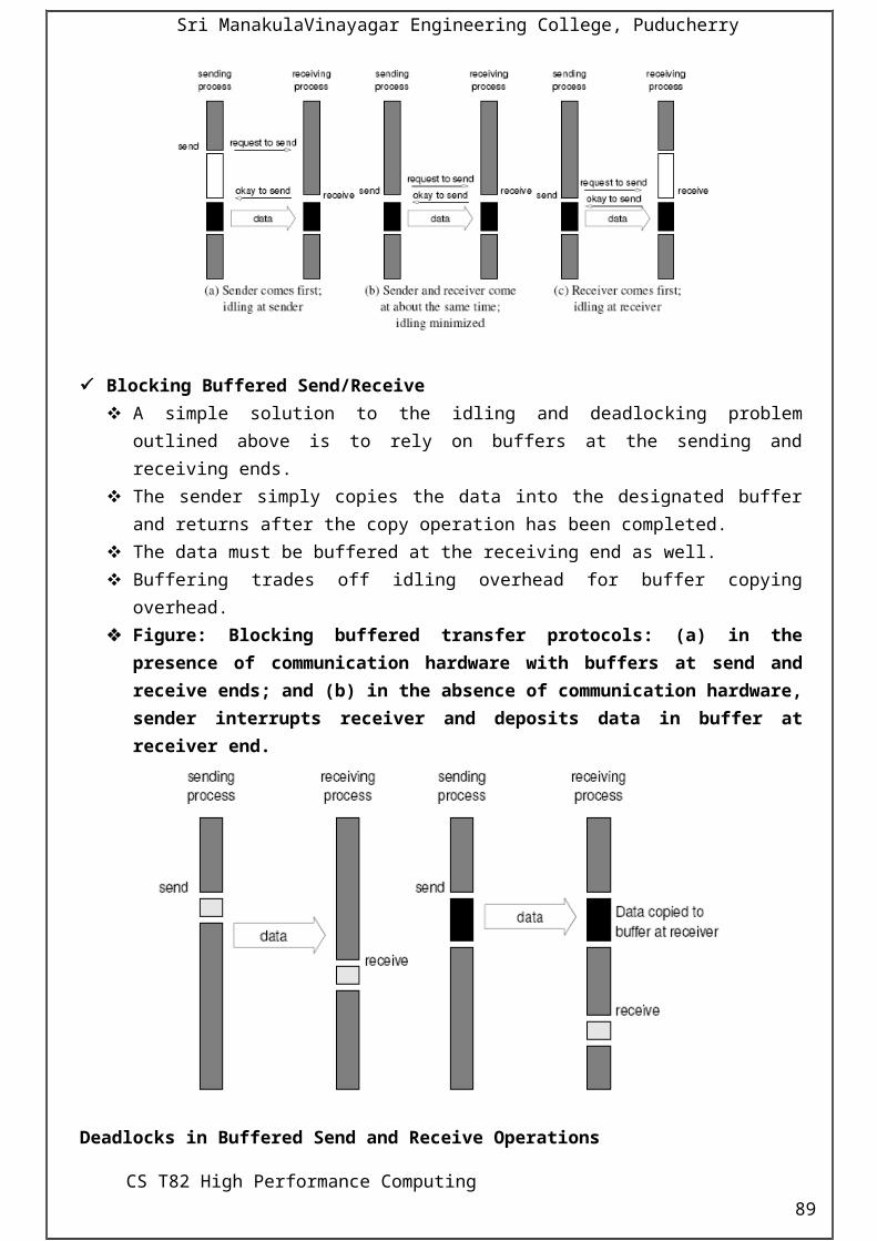
Sri ManakulaVinayagar Engineering College, Puducherry
In the first phase (which is similar to the shared-address-space formulation), the locally stored
array Ai at process Pi is partitioned into the smaller-than- and larger-than-the-pivot sub-arrays
Si and Li locally.
In the next phase, the algorithm first determines which processes will be responsible for
recursively sorting the smaller-than-the-pivot sub-arrays and which process will be
responsible for recursively sorting the larger-than-the-pivot sub-arrays
Once this is done, then the processes send theirS i and Li arrays to the corresponding
processes. After that, the processes are partitioned into the two groups, one for S and one for
L, and the algorithm proceeds recursively.
The recursion terminates when each sub-array is assigned to a single process, at which point it
is sorted locally.
Thus, the overall complexity for the split is Q(n/p) + Q(log p).
Pivot Selection
Pivot selection is particularly difficult, and it significantly affects the algorithm's performance.
In the parallel formulation, however, one poor pivot may lead to a partitioning in which a
process becomes idle, and that will persist throughout the execution of the algorithm.
If the initial distribution of elements in each process is uniform, then a better pivot selection
method can be derived.
Since the distribution of elements on each process is the same as the overall distribution of the
n elements, the median selected to be the pivot during the first step is a good approximation of
the overall median. Since the selected pivot is very close to the overall median, roughly half
of the elements in each process are smaller and the other half larger than the pivot.
Therefore, the first split leads to two partitions, such that each of them has roughly n/2
elements. Similarly, the elements assigned to each process of the group that is responsible for
sorting the smaller-than-the-pivot elements (and the group responsible for sorting the larger-
than-the-pivot elements) have the same distribution as the n/2 smaller (or larger) elements of
the original list.
Thus, the split not only maintains load balance but also preserves the assumption of uniform
element distribution in the process group.
Therefore, the application of the same pivot selection scheme to the sub-groups of processes
continues to yield good pivot selection.
CS T82 High Performance Computing 89

Sri ManakulaVinayagar Engineering College, Puducherry
5. By defining what a minimum spanning tree is explain the Prim’s sequential and parallel
algorithms. Also mention their complexity. (November 2013)
A spanning tree of an undirected graph G is a subgraph of G that is a tree containing all the
vertices of G. In a weighted graph, the weight of a subgraph is the sum of the weights of the
edges in the subgraph.
A minimum spanning tree (MST) for a weighted undirected graph is a spanning tree with
minimum weight. Many problems require finding an MST of an undirected graph.
Figure: An undirected graph and its minimum spanning tree.
If G is not connected, it cannot have a spanning tree. Instead, it has a spanning forest.
Prim's algorithm for finding an MST is a greedy algorithm. The algorithm begins by selecting
an arbitrary starting vertex. It then grows the minimum spanning tree by choosing a new
vertex and edge that are guaranteed to be in a spanning tree of minimum cost.
The algorithm continues until all the vertices have been selected.
Let G = (V, E, w) be the weighted undirected graph for which the minimum spanning tree is to
be found, and leAt = (ai, j) be its weighted adjacency matrix.
Figure: Prim's minimum spanning tree algorithm. The MST is rooted at vertex b. For
each iteration, vertices in VT as well as the edges selected so far are shown in bold. The
array d[v] shows the values of the vertices in V - VT after they have been updated.
CS T82 High Performance Computing 90

Sri ManakulaVinayagar Engineering College, Puducherry
Algorithm: Prim's sequential minimum spanning tree algorithm.
1. procedurePRIM_MST(V, E, w, r)
2. begin
CS T82 High Performance Computing 91

Sri ManakulaVinayagar Engineering College, Puducherry
3. VT := {r};
4. d[r] := 0;
5. for all v (V - VT )do
6. ifedge (r, v) exists set d[v] := w(r, v);
7. elseset d[v] := ;
8. whileVT V do
9. begin
10. find a vertex u such that d[u] :=min{d[v]|v (V - VT )};
11. VT :=VT {u};
12. for all v (V - VT )do
13. d[v] := min{d[v], w(u, v)};
14. endwhile
15. endPRIM_MST
Thus, the total communication cost of each iteration is Q(log p). The parallel run time of this formulation is given by
Since the sequential run time is W = Q(n2), the speedup and efficiency are as follows:
6. Write and explain the single source shortest path. (6 marks)
For a weighted graph G = (V, E, w), the single-source shortest paths problem is to find the
shortest paths from a vertex v V to all other vertices in V. A shortest path from u to v is a minimum-weight path.
Depending on the application, edge weights may represent time, cost, penalty, loss, or any other quantity that accumulates additively along a path and is to be minimized.
Here, we present Dijkstra's algorithm, which solves the single-source shortest-paths problem on both directed and undirected graphs with non-negative weights.
Dijkstra's algorithm, which finds the shortest paths from a single vertex s, is similar to Prim's minimum spanning tree algorithm.
CS T82 High Performance Computing 92
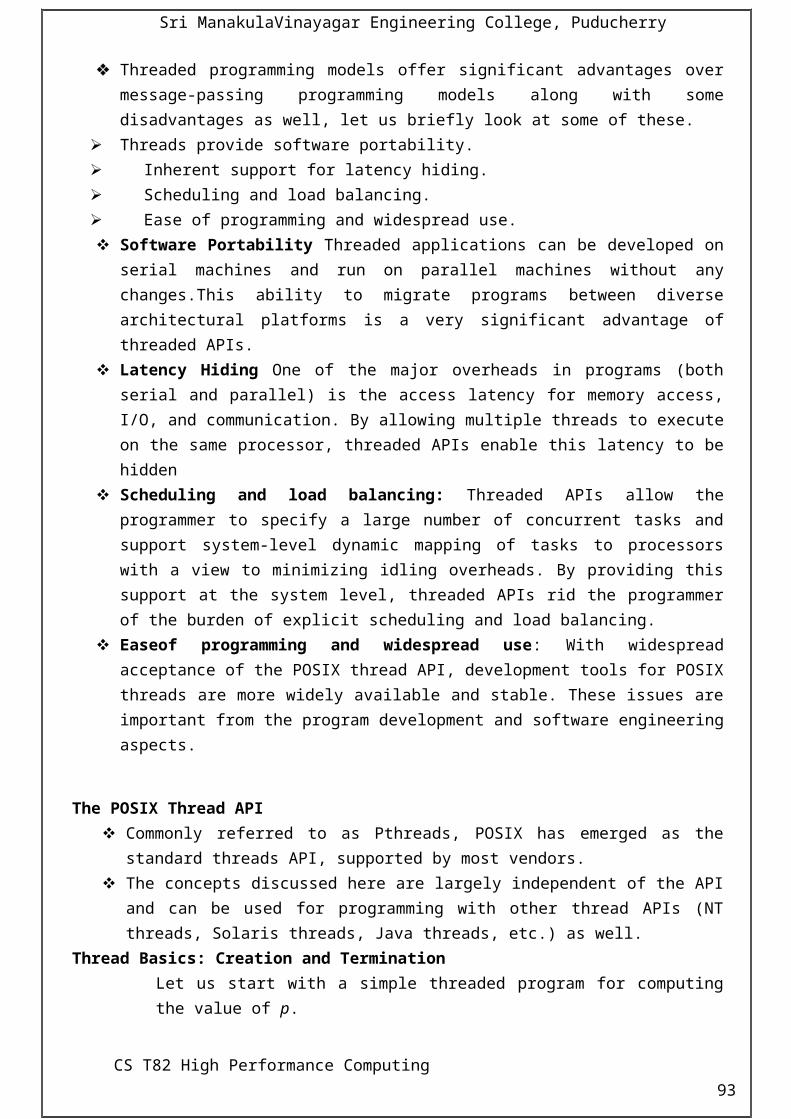
Sri ManakulaVinayagar Engineering College, Puducherry
The main difference is that, for each vertex u (V - VT ), Dijkstra's algorithm stores l[u], the minimum cost to reach vertex u from vertex s by means of vertices in VT; Prim's algorithm stores d [u], the cost of the minimum-cost edge connecting a vertex in VT to u. The run time of Dijkstra's algorithm is Q(n2).
Algorithm: Dijkstra's sequential single-source shortest paths algorithm.
1. procedureDIJKSTRA_SINGLE_SOURCE_SP(V, E, w, s)
2. begin
3. VT := {s};
4. for all v (V - VT )do
5. if(s, v) exists set l[v] := w(s, v);
6. elseset l[v] := ;
7. whileVT V do
8. begin
9. find a vertex u such that l[u] := min{l[v]|v (V - VT )};
10. VT :=VT {u};
11. for all v (V - VT )do
12. l[v] := min{l[v], l[u] + w(u, v)};
13. endwhile
14. endDIJKSTRA_SINGLE_SOURCE_SP
Dijkstra's Algorithm in parallel formulations:
This algorithm can also be used to solve the all-pairs shortest paths problem by executing the single-source algorithm on each process, for each vertex v.
We refer to this algorithm as Dijkstra's all-pairs shortest paths algorithm. Since the complexity of Dijkstra's single-source algorithm is Q (n2), the complexity of the all-pairs algorithm is Q (n3).Parallel Formulations
Dijkstra's all-pairs shortest paths problem can be parallelized in two distinct ways. One approach partitions the vertices among different processes and has each process
compute the single-source shortest paths for all vertices assigned to it. We refer to this approach as the source-partitioned formulation.
Another approach assigns each vertex to a set of processes and uses the parallel formulation of the single-source algorithm to solve the problem on each set of processes. We refer to this approach as the source-parallel formulation.
Thus, the parallel run time of source-partitioned formulation is given by
CS T82 High Performance Computing 93

Sri ManakulaVinayagar Engineering College, Puducherry
Thus, the parallel run time of source-parallel formulation is given by
7. Explain and write the parallel algorithms of Floyd’s algorithm.
Let G = (V, E, w) be the weighted graph, and let V = {v1,v2,..., vn} be the vertices of G.
Consider a subset {v1, v2,...,vk} of vertices for some k where k n.
For any pair of vertices vi ,vj V, consider all paths from vi to vjwhose intermediate vertices
belong to the set {v1, v2,..., vk}. Let be the minimum-weight path among them, and let
be the weight of .
If vertex vkis not in the shortest path from vito v j, then is the same as .
However, if v k is in , then we can break into two paths – one from vi to vkand one from vkto vj. Each of these paths uses vertices from {v1, v2,...,vk-1}.
Thus, . These observations are expressed in the following recurrence equation:
Algorithm:Floyd's all-pairs shortest paths algorithm. This program computes the all-pairs shortest paths of the graph G = (V, E ) with adjacency matrix A.
1. procedure FLOYD_ALL_PAIRS_SP(A)
2. begin
3. D(0) = A;
4. for k := 1 to ndo
5. for i := 1 to ndo
6. for j := 1 to ndo
CS T82 High Performance Computing 94
Sri ManakulaVinayagar Engineering College, Puducherry
7.
8. endFLOYD_ALL_PAIRS_SP
Parallel Formulation
A generic parallel formulation of Floyd's algorithm assigns the task of computing matrix D (k) for each value of k to a set of processes.
Let p be the number of processes available. Matrix D (k) is partitioned into p parts, and each part is assigned to a process.
Each processcomputes the D (k) values of its partition. To accomplish this, a process must access the corresponding segments of the kthrow and
column of matrix D(k-1) A simple example of 2-D block mapping algorithm is shown below:
Algorithm: Floyd's parallel formulation using the 2-D block mapping. P*,jdenotes all the processes in the jth column, and Pi,* denotes all the processes in the ith row. The matrix D(0) is the adjacency matrix.
1. procedureFLOYD_2DBLOCK(D(0))
2. begin
3. for k := 1 to ndo
4. begin
5. each process Pi,jthat has a segment of the kth row of D(k-1);
broadcasts it to the P*,j processes;
6. each process Pi,jthat has a segment of the kth column of D(k-1);
broadcasts it to the Pi,* processes;
7. each process waits to receive the needed segments;
8. each process Pi,jcomputes its part of the D(k) matrix;
9. end
10. endFLOYD_2DBLOCK
Table 1:The performance and scalability of the all-pairs shortest paths algorithms on various
architectures with O (p) bisection bandwidth. Similar run times apply to all k - d cube
architectures, provided that processes are properly mapped to the underlying processors.
CS T82 High Performance Computing 95
Sri ManakulaVinayagar Engineering College, Puducherry
UNIT – IV
QUESTION BANK
2 MARKS
1. What is a dense matrix algorithm?
2. Define Bitonic Sequence. (November 2013)
3. Write Matrix vector multiplication algorithm.
4. What is block matrices operations?
5. What is DNS algorithm?
6. What is LU Factorization?
7. What is pipelined Gaussian elimination?
8. What is partial pivoting?
9. What is scaled speedup?
10. What is sorting?
11. Types of sorting?
12. What is internal sorting?
13. What is external sorting?
14. What is comparison based algorithm?
15. What is comparator?
16. Types of comparator?
17. What is Bitonic sort? (November 2013)
18. What is shell sort?
19. What is quick sort?
20. What is bucket sort?
21. What is sample sort?
22. What is spanning tree?
23. What is weighted graph?
CS T82 High Performance Computing 96

Sri ManakulaVinayagar Engineering College, Puducherry
24. What is minimum spanning tree? (April 2013)
25. What is shortest path?
26. What is connected components?
27. Define sorting networks (April 2013)
11 MARKS1. Explain how the parallel implementation of Gaussian elimination algorithm is used in solving
a system of linear equations. (November 2013) (Ref.Pg.No.78)2. Explain in detail Matrix vector multiplication. (April 2013) (Ref.Pg.No.80)3. Discuss in cannon’s and DNS algorithm in details.4. Explain in detail about quick sort in parallel ( April 2013) (Ref.Pg.No.86)5. By defining what a minimum spanning tree is explain the Prim’s sequential and parallel
algorithms. Also mention their complexity. (November 2013) (Ref.Pg.No.89)6. Write and explain the single source shortest path. (6 marks)7. Explain and write the parallel algorithms of Floyd’s algorithm.
CS T82 High Performance Computing 97

Sri ManakulaVinayagar Engineering College, Puducherry
UNIT - V
Search Algorithms for Discrete for Discrete Optimization Problems:
Definitions and examples Sequential search algorithms Search overhead factor Parallel depth-first search Parallel best-first search Speedup anomalies in parallel search algorithms.
Dynamic Programming: Overview.
TWO MARKS
1. Define discrete optimization problem ?( April 2013/December 2013)
A discrete optimization problem can be expressed as a tuple (S, f). The set S is a finite or
countably infinite set of all solutions that satisfy specified constraints. This set is called the set of
feasible solutions. The function f is the cost function that maps each element in set S onto the set of
real numbers R. f: S -> R
2. What is a 8-Puzzle problem?
The 8-puzzle problem consists of a 3 x 3 grid containing eight tiles, numbered one through
eight. One of the grid segments (called the "blank") is empty.
A tile can be moved into the blank position from a position adjacent to it, thus creating
a blank in the tile's original position.
Depending on the configuration of the grid, up to four moves are possible: up, down,
left, and right. The initial and final configurations of the tiles are specified.
The objective is to determine a shortest sequence of moves that transforms the initial
configuration to the final configuration.
3. Define the following terminal node, non-terminal node?
Terminal node is a node that has no successors and all other nodes apart from terminal nodes
are called as non terminal nodes
4. What is a state space?
The nodes of a graph are called states the cost of a path is the sum of the edge costs. Such a
graph is called a state space.
5. What is sequential search algorithm? (April 2013)
The sequential search examines the first element in the list and then examines each sequential
element in the list until a match is found. This match could be desired word that you are searching
for, or minimum number in the list
CS T82 High Performance Computing 98

Sri ManakulaVinayagar Engineering College, Puducherry
6. What are the various types of sequential search algorithms?
The various types of sequential search algorithms are
Depth First Search Algorithm
Best First Search Algorithm
7. Define DFS?
Depth-first search (DFS) is an algorithm for traversing or searching a tree, tree structure,
or graph. DFS begins by expanding the initial node and generating its successors. In each subsequent
step, DFS expands one of the most recently generated nodes. If this node has no successors then DFS
backtracks and expands a different node. In some DFS algorithms, successors of a node are expanded
in an order determined by their heuristic values.
8. What is backtracking?
Simple backtracking is a depth-first search method that terminates upon finding the first
solution. Thus, it is not guaranteed to find a minimum-cost solution. Simple backtracking uses no
heuristic information to order the successors of an expanded node. A variant, ordered backtracking,
does use heuristics to order the successors of an expanded node.
9. Define DFBB?
Depth-first branch-and-bound (DFBB) exhaustively searches the state space; that is, it
continues to search even after finding a solution path. Whenever it finds a new solution path, it
updates the current best solution path. DFBB discards inferior partial solution paths (that is, partial
solution paths whose extensions are guaranteed to be worse than the current best solution path). Upon
termination, the current best solution is a globally optimal solution.
10. Define iterative Deepening A*?
DFS algorithm may get stuck searching a deep part of the search space when a solution exists
higher up on another branch. For such trees, we impose a bound on the depth to which the DFS
algorithm searches. If the node to be expanded is beyond the depth bound, then the node is not
expanded and the algorithm backtracks. If a solution is not found, then the entire state space is
searched again using a larger depth bound. This technique is called iterative deepening depth-first
search
11. What is BFS?
Best-first search (BFS) algorithms can search both graphs and trees. These algorithms use
heuristics to direct the search to portions of the search space likely to yield solutions. Smaller
heuristic values are assigned to more promising nodes. BFS maintains two lists: open and closed.
12. What are the important parameters of Parallel Depth – First Search?
The important parameters of paralled DFS are the following
Work-Splitting Strategies
Load-Balancing Schemes
CS T82 High Performance Computing 99
Sri ManakulaVinayagar Engineering College, Puducherry
13. What is search overhead factor?
Let Wpbe the amount of work done by a single processor, and Wpbe the total amount of work
done by p processors. The search overhead factor of the parallel system is defined as the ratio of the
work done by the parallel formulation to that done by the sequential formulation, or Wp/W
14. What do you mean by lwork splitting strategies?
When work is transferred, the donor's stack is split into two stacks, one of which is sent to the
recipient. In other words, some of the nodes are removed from the donor's stack and added to the
recipient's stack. If too little work is sent, the recipient quickly becomes idle; if too much, the donor
becomes idle. Ideally, the stack is split into two equal pieces such that the size of the search space
represented by each stack is the same. Such a split is called a half-split.
15. Define parallel BFS?
Most important component of best-first search (BFS) algorithms is the open list. It maintains
the unexpanded nodes in the search graph, ordered according to their l-value. In the sequential
algorithm, the most promising node from the open list is removed and expanded, and newly generated
nodes are added to the open list. In most parallel formulations of BFS, different processors
concurrently expand different nodes from the open list.
16. What is the communication Strategies for Parallel Best-First Tree Search?
The communication strategies for parallel BFS are
Random communication strategy
Ring communication strategy
Blackboard communication strategy
17. Define random communication strategy?
In the random communication strategy, each processor periodically sends some of its
best nodes to the open list of randomly selected processor.
This strategy ensures that, if a processor stores a good part of the search space, the
others get part of it. If nodes are transferred frequently, the search overhead factor can
be made very small; otherwise it can become quite large.
The communication cost determines the best node transfer frequency. If the
communication cost is low, it is best to communicate after every node expansion.
CS T82 High Performance Computing 100
Sri ManakulaVinayagar Engineering College, Puducherry
18. Illustrate the Blackboard communication strategy?
19. What is Speedup Anomalies in Parallel Search Algorithms?
In parallel search algorithms, speedup can vary greatly from one execution to another because
the portions of the search space examined by various processors are determined dynamically and can
differ for each execution.’ The order of node expansions is indicated by node labels. The sequential
formulation generates 13 nodes before reaching the goal node G.
20. Define Dynamic programming?( April/May 2013)
Dynamic programming (DP) is a commonly used technique for solving a wide variety of
discrete optimization problems such as scheduling, string-editing, packaging, and inventory
management.. DP views a problem as a set of interdependent subproblems. It solves subproblems and
uses the results to solve larger subproblems until the entire problem is solved.
CS T82 High Performance Computing 101

Sri ManakulaVinayagar Engineering College, Puducherry
11 MARKS
1. Explain sequential search algorithm?
The most suitable sequential search algorithm to apply to a state space depends on whether the space forms a graph or a tree.
In a tree, each new successor leads to an unexplored part of the search space. An example of this is the 0/1 integer-programming problem.
In a graph, however, a state can be reached along multiple paths. An example of such a problem is the 8-puzzle.
For such problems, whenever a state is generated, it is necessary to check if the state has already been generated. If this check is not performed, then effectively the search graph is unfolded into a tree in which a state is repeated for every path that leads to it (Figure).
Figure: Two examples of unfolding a graph into a tree.
For many problems (for example, the 8-puzzle), unfolding increases the size of the search space by a small factor.
For some problems, however, unfolded graphs are much larger than the original graphs. Figure illustrates a graph whose corresponding tree has an exponentially higher number of
states. In this section, we present an overview of various sequential algorithms used to solve DOPs that are formulated as tree or graph search problems.
2. Explain In Detail About Depth-First Search With Example?
Depth-first search (DFS) algorithms solve DOPs that can be formulated as tree-search
problems. DFS begins by expanding the initial node and generating its successors. In each subsequent
step, DFS expands one of the most recently generated nodes. If this node has no successors (or cannot
lead to any solutions), then DFS backtracks and expands a different node.
CS T82 High Performance Computing 102

Sri ManakulaVinayagar Engineering College, Puducherry
In some DFS algorithms, successors of a node are expanded in an order determined by their
heuristic values. A major advantage of DFS is that its storage requirement is linear in the depth of the
state space being searched. The following sections discuss three algorithms based on depth-first
search.
Simple Backtracking
Simple backtracking is a depth-first search method that terminates upon finding the first
solution. Thus, it is not guaranteed to find a minimum-cost solution. Simple backtracking uses no
heuristic information to order the successors of an expanded node. A variant, ordered backtracking,
does use heuristics to order the successors of an expanded node.
Depth-First Branch-and-Bound
Depth-first branch-and-bound (DFBB) exhaustively searches the state space; that is, it
continues to search even after finding a solution path. Whenever it finds a new solution path, it
updates the current best solution path. DFBB discards inferior partial solution paths (that is, partial
solution paths whose extensions are guaranteed to be worse than the current best solution path). Upon
termination, the current best solution is a globally optimal solution.
Iterative Deepening A*
Trees corresponding to DOPs can be very deep. Thus, a DFS algorithm may get stuck
searching a deep part of the search space when a solution exists higher up on another branch. For
such trees, we impose a bound on the depth to which the DFS algorithm searches. If the node to be
expanded is beyond the depth bound, then the node is not expanded and the algorithm backtracks. If a
solution is not found, then the entire state space is searched again using a larger depth bound. This
technique is called iterative deepening depth-first search (IDDFS).
Note that this method is guaranteed to find a solution path with the fewest edges. However, it is not
guaranteed to find a least-cost path.
Iterative deepening A* (IDA*) is a variant of ID-DFS. IDA* uses the l-values of nodes to
bound depth (recall from Section 11.1 that for node x, l(x) = g(x) + h(x)). IDA* repeatedly performs
cost-bounded DFS over the search space. In each iteration, IDA* expands nodes depth-first. If the l-
value of the node to be expanded is greater than the cost bound, then IDA*backtracks. If a solution is
not found within the current cost bound, then IDA* repeats the entire depth-first search using a higher
cost bound. In the first iteration, the cost bound is set to the l value of the initial state s. Note that
since g(s) is zero, l(s) is equal to h(s). In each subsequent iteration, the cost bound is increased. The
new cost bound is equal to the minimum l-value of the nodes that were generated but could not be
CS T82 High Performance Computing 103

Sri ManakulaVinayagar Engineering College, Puducherry
expanded in the previous iteration. The algorithm terminates when a goal node is expanded. IDA* is
guaranteed to find an optimal solution if the heuristic function is admissible. It may appear that IDA*
performs a lot of redundant work across iterations. However, for many problems the redundant work
performed by IDA* is minimal, because most of the work is done deep in the search space.
Example: Depth-first search: the 8-puzzle
Figure shows the execution of depth-first search for solving the 8-puzzleproblem. The search
starts at the initial configuration. Successors of this state are generated by applying possible moves.
During each step of the search algorithm anew state is selected, and its successors are generated. The
DFS algorithm expands the deepest node in the tree. In step 1, the initial state A generates states B
and C. One of these is selected according to a predetermined criterion. In the example, we order
successors by applicable moves as follows: up, down, left, and right. In step 2,the DFS algorithm
selects state B and generates states D, E, and F. Note that the state D can be discarded, as it is a
duplicate of the parent of B. In step 3, state E is expanded to generate states G and H. Again G can be
discarded because it is a duplicate of B. The search proceeds in this way until the algorithm
backtracks or the final configuration is generated.
Figure: States resulting from the first three steps of
Depth-first search applied to an instance of the 8-puzzle.
In each step of the DFS algorithm, untried alternatives must be stored. For example, in the 8-puzzle
problem, up to three untried alternatives are stored at each step. In general, if m is the amount of
storage required to store a state, and d is the maximum depth, then the total space requirement of the
DFS algorithm is O (md). The state-space tree searched by parallel DFS can be efficiently represented
CS T82 High Performance Computing 104

Sri ManakulaVinayagar Engineering College, Puducherry
as a stack. Since the depth of the stack increases linearly with the depth of the tree, the memory
requirements of a stack representation are low.
There are two ways of storing untried alternatives using a stack.
In the first representation, untried alternates are pushed on the stack at each step. The
ancestors of a state are not represented on the stack. Figure (b) illustrates this representation
for the tree shown in Figure (a).
In the second representation, shown in Figure (c), untried alternatives are stored along with
their parent state. It is necessary to use the second representation if the sequence of
transformations from the initial state to the goal state is required as a part of the solution.
Furthermore, if the state space is a graph in which it is possible to generate an ancestor state by
applying a sequence of transformations to the current state, then it is desirable to use the second
representation, because it allows us to check for duplication of ancestor states and thus remove any
cycles from the state-space graph. The second representation is useful for problems such as the 8-
puzzle. In Example 11.5, using the second representation allows the algorithm to detect that nodes D
and G should be discarded.
Figure: Representing a DFS tree: (a) the DFS tree; successor nodes shown with dashed lines
have already been explored; (b) the stack storing untried alternatives only; and (c) the stack
storing untried alternatives along with their parent. The shaded blocks represent the parent
state and the block to the right represents successor states that have not been explored.
CS T82 High Performance Computing 105

Sri ManakulaVinayagar Engineering College, Puducherry
3. Explain About Best-First Search Algorithms With Example?
Best-first search (BFS) algorithms can search both graphs and trees. These algorithms use heuristics to direct the search to portions of the search space likely to yield solutions. Smaller heuristic values are assigned to more promising nodes.
BFS maintains two lists: open and closed.
At the beginning, the initial node is placed on the open list. This list is sorted according to a heuristic evaluation function that measures how likely each node is to yield a solution. In each step of the search, the most promising node from the open list is removed. If this node is a goal node, then the algorithm terminates. Otherwise, the node is expanded.
The expanded node is placed on the closed list. The successors of the newly expanded node are placed on the open list under one of the following circumstances: (1) the successor is not already on the open or closed lists, and (2) the successor is already on the open or closed list but has a lower heuristic value. In the second case, the node with the higher heuristic value is deleted.
A common BFS technique is the A* algorithm. The A* algorithm uses the lower bound function l as a heuristic evaluation function. Recall from Section 11.1 that for each node x ,l(x) is the sum of g(x) and h(x). Nodes in the open list are ordered according to the value of the l function.
At each step, the node with the smallest l-value (that is, the best node) is removed from the open list and expanded. Its successors are inserted into the open list at the proper positions and the node itself is inserted into the closed list. For an admissible heuristic function, A* finds an optimal solution.
The main drawback of any BFS algorithm is that its memory requirement is linear in the size of the search space explored. For many problems, the size of the search space is exponential in the depth of the tree expanded. For problems with large search spaces, memory becomes alimitation.
Example Best-first search: the 8-puzzle
Consider the 8-puzzle problem from Examples 11.2 and 11.4. Figure 11.6 illustrates four steps of best-first search on the 8-puzzle. At each step, a state x with the minimum l-value (l(x) = g(x) + h(x)) is selected for expansion. Ties are broken arbitrarily. BFS can check for a duplicate nodes, since all previously generated nodes are kept on either the open or closed list.
Figure: Applying best-first search to the 8-puzzle: (a)initial configuration; (b) final configuration; and (c) states resulting from the first four steps of best-first search. Each state is labeled with its h-value (that is, the Manhattan distance from the state to the final state).
CS T82 High Performance Computing 106

Sri ManakulaVinayagar Engineering College, Puducherry
4. Explain In Detail About Search Overhead Factor? (6 MARKS)
Parallel search algorithms incur overhead from several sources. These include communication overhead, idle time due to load imbalance, and contention for shared data structures. Thus, if both the sequential and parallel formulations of an algorithm do the same amount of work, the speedup of parallel search on p processors is less than p. However, the amount of work done by a parallel formulation is often different from that done by the corresponding sequential formulation because they may explore different parts of the search space.
Let W be the amount of work done by a single processor, and Wpbe the total amount of work done by p processors. The search overhead factor of the parallel system is defined as the ratio of the work done by the parallel formulation to that done by the sequential formulation, or Wp/W. Thus, the upper bound on speedup for the parallel system is given by p x(W/Wp). The actual speedup, however, may be less due to other parallel processing overhead. In most parallel search algorithms, the search overhead factor is greater than one. However, in some cases, it may be less than one, leading to superlinear speedup. If the search overhead factor is less than one on the average, then it indicates that the serial search algorithm is not the fastest algorithm for solving the problem.
To simplify our presentation and analysis, we assume that the time to expand each node is the same, and W and Wpare the number of nodes expanded by the serial and the parallel formulations, respectively. If the time for each expansion is tc, then the sequential run time is given by TS =
CS T82 High Performance Computing 107

Sri ManakulaVinayagar Engineering College, Puducherry
tcW. In the remainder of the chapter, we assume that tc= 1. Hence, the problem sizeW and the serial run time TS become the same.
5. Explain in detail about parallel depth-first search? ( April 2013) (November 2013)
The critical issue in parallel depth-first search algorithms is the distribution of the search space among the processors. Consider the tree shown in Figure 11.7. Note that the left subtree (rooted at node A) can be searched in parallel with the right subtree (rooted at node B). By statically assigning a node in the tree to a processor, it is possible to expand the whole subtree rooted at that node without communicating with another processor. Thus, it seems that such a static allocation yields a good parallel search algorithm.
Figure: The unstructured nature of tree search and the imbalance resulting from static partitioning.
Let us see what happens if we try to apply this approach to the tree in Figure 11.7. Assume that we have two processors. The root node is expanded to generate two nodes (A and B), and each of these nodes is assigned to one of the processors. Each processor now searches the subtrees rooted at its assigned node independently. At this point, the problem with static node assignment becomes apparent. The processor exploring the subtree rooted at node A expands considerably fewer nodes than does the other processor. Due to this imbalance in the workload, one processor is idle for a significant amount of time, reducing efficiency. Using a larger number of processors worsens the imbalance. Consider the partitioning of the tree for four processors.
Nodes A and B are expanded to generate nodes C, D, E, and F. Assume that each of these nodes is assigned to one of the four processors. Now the processor searching the subtree rooted at node E does most of the work, and those searching the subtrees rooted at nodes C and D spend most of their time
CS T82 High Performance Computing 108

Sri ManakulaVinayagar Engineering College, Puducherry
idle. The static partitioning of unstructured trees yields poor performance because of substantial variation in the size of partitions of the search space rooted at different nodes. Furthermore, since the search space is usually generated dynamically, it is difficult to get a good estimate of the size of the search space beforehand. Therefore, it is necessary to balance the search space among processors dynamically.
In dynamic load balancing, when a processor runs out of work, it gets more work from another processor that has work. Consider the two-processor partitioning of the tree in Figure (a). Assume that nodes A and B are assigned to the two processors as we just described. In this case when the processor searching the subtree rooted at node A runs out of work, it requests work from the other processor. Although the dynamic distribution of work results in communication overhead for work requests and work transfers, it reduces load imbalance among processors. This section explores several schemes for dynamically balancing the load between processors.
A parallel formulation of DFS based on dynamic load balancing is as follows. Each processor performs DFS on a disjoint part of the search space. When a processor finishes searching its part of the search space, it requests an unsearched part from other processors. This takes the form of work request and response messages in message passing architectures, and locking and extracting work in shared address space machines. Whenever a processor finds a goal node, all the processors terminate. If the search space is finite and the problem has no solutions, then all the processors eventually run out of work, and the algorithm terminates.
Since each processor searches the state space depth-first, unexplored states can be conveniently stored as a stack. Each processor maintains its own local stack on which it executes DFS. When a processor's local stack is empty, it requests (either via explicit messages or by locking) untried alternatives from another processor's stack. In the beginning, the entire search space is assigned to one processor, and other processors are assigned null search spaces (that is, empty stacks). The search space is distributed among the processors as they request work. We refer to the processor that sends work as the donor processor and to the processor that requests and receives work as the recipient processor.
As illustrated in Figure each processor can be in one of two states: active (that is, it has work) or idle (that is, it is trying to get work). In message passing architectures, an idle processor selects a donor processor and sends it a work request. If the idle processor receives work (part of the state space to be searched) from the donor processor, it becomes active. If it receives a reject message (because the donor has no work), it selects another donor and sends a work request to that donor. This process repeats until the processor gets work or all the processors become idle. When a processor is idle and it receives a work request, that processor returns a reject message. The same process can be implemented on shared address space machines by locking another processors' stack, examining it to see if it has work, extracting work, and unlocking the stack.
Figure: A generic scheme for dynamic load balancing.
CS T82 High Performance Computing 109

Sri ManakulaVinayagar Engineering College, Puducherry
On message passing architectures, in the active state, a processor does a fixed amount of work (expands a fixed number of nodes) and then checks for pending work requests. When a work request is received, the processor partitions its work into two parts and sends one part to the requesting processor. When a processor has exhausted its own search space, it becomes idle.
This process continues until a solution is found or until the entire space has been searched. If a solution is found, a message is broadcast to all processors to stop searching. A termination detection algorithm is used to detect whether all processors have become idle without finding a solution
Important Parameters of Parallel DFS
Two characteristics of parallel DFS are critical to determining its performance. First is the method for splitting work at a processor, and the second is the scheme to determine the donor processor when a processor becomes idle.
Work-Splitting Strategies
When work is transferred, the donor's stack is split into two stacks, one of which is sent to the recipient. In other words, some of the nodes (that is, alternatives) are removed from the donor's stack and added to the recipient's stack. If too little work is sent, the recipient quickly becomes idle; if too much, the donor becomes idle. Ideally, the stack is split into two equal pieces such that the size of the search space represented by each stack is the same. Such a split is called a half-split. It is difficult to get a good estimate of the size of the tree rooted at an unexpanded alternative in the stack. However, the alternatives near the bottom of the stack (that is, close to the initial node) tend to have bigger trees rooted at them, and alternatives near the top of the stack tend to have small trees rooted at them. To
CS T82 High Performance Computing 110

Sri ManakulaVinayagar Engineering College, Puducherry
avoid sending very small amounts of work, nodes beyond a specified stack depth are not given away. This depth is called the cutoff depth.
Some possible strategies for splitting the search space are (1) send nodes near the bottom of the stack, (2) send nodes near the cutoff depth, and (3) send half the nodes between the bottom of the stack and the cutoff depth. The suitability of a splitting strategy depends on the nature of the search space. If the search space is uniform, both strategies 1 and 3 work well. If the search space is highly irregular, strategy 3 usually works well. If a strong heuristic is available (to order successors so that goal nodes move to the left of the state-space tree), strategy 2 is likely to perform better, since it tries to distribute those parts of the search space likely to contain a solution. The cost of splitting also becomes important if the stacks are deep .For such stacks, strategy 1 has lower cost than strategies 2 and 3.
Figure: shows the partitioning of the DFS tree of Figure 11.5(a)into two subtrees using strategy 3. Note that the states beyond the cutoff depth are not partitioned. Figure 11.9alsoshows the representation of the stack corresponding to the two subtrees. The stack representation used in the figure stores only the unexplored alternatives.
Figure: Splitting the DFS tree in Figure 11.5. The two subtrees along with their stack representations are shown in (a) and (b).
This section discusses three dynamic load-balancing schemes: asynchronous round robin, global round robin, and random polling. Each of these schemes can be coded for message passing as well as shared address space machines. Asynchronous Round Robin In asynchronous round robin (ARR), each processor maintains an independent variable, target. Whenever a processor runs out of work, it uses target as the label of a donor processor and attempts to get work from it. The value of target is incremented (modulo p) each time a work request is sent. The initial value of target at each processor is set to ((label+ 1) modulo p) where label is the local processor label. Note that work requests are
CS T82 High Performance Computing 111

Sri ManakulaVinayagar Engineering College, Puducherry
generated independently by each processor. However, it is possible for two or more processors to request work from the same donor at nearly the same time.
Global Round Robin Global round robin (GRR) uses a single global variable called target. This variable can be stored in a globally accessible space in shared address space machines or at a designated processor in message passing machines. Whenever a processor needs work, it requests and receives the value of target, either by locking, reading, and unlocking on shared address space machines or by sending a message requesting the designated processor (say P0).
The value of target is incremented (modulo p) before responding to the next request. The recipient processor then attempts to get work from a donor processor whose label is the value of target. GRR ensures that successive work requests are distributed evenly over all processors. A drawback of this scheme is the contention for access to target.
Random PollingRandom polling (RP) is the simplest load-balancing scheme. When a processor becomes idle, it randomly selects a donor. Each processor is selected as a donor with equal probability, ensuring that work requests are evenly distributed.
6. Explain About Dynamic Programming? (April 2013)
Dynamic programming (DP) is a commonly used technique for solving a wide variety of
discrete optimization problems such as scheduling, string-editing, packaging, and inventory
management. More recently, it has found applications in bioinformatics in matching sequences of
amino-acids and nucleotides (the Smith-Waterman algorithm). DP views a problem as a set of
interdependent sub problems. It solves sub problems and uses the results to solve larger sub problems
until the entire problem is solved. In contrast to divide-and-conquer, where the solution to a problem
depends only on the solution to its sub problems, in DP there may be interrelationships across sub
problems. In DP, the solution to a sub problem is expressed as a function of solutions to one or more
sub problems at the preceding levels.
Overview of Dynamic programming
Example 12.1 the shortest-path problem
Consider a DP formulation for the problem of finding a shortest (least-cost) path between a pair of vertices in an acyclicgraph. (Refer to Section 10.1 for an introduction to graph terminology.) An edge connecting node i to node j has cost c(i,j). If two vertices i and j are not connected then c(i, j) = . The graph contains n nodes numbered 0, 1, ...,n - 1, and has an edge from node i to node j only if i <j. The shortest-path problem is to find a least-cost path between nodes 0 and n - 1. Let f (x) denote the cost of the least-cost path from node 0 to node x. Thus, f (0) is zero, and finding f (n - 1) solves the problem. The DP formulation for this problem yields the following recursive equations for f (x):
CS T82 High Performance Computing 112
Sri ManakulaVinayagar Engineering College, Puducherry
As an instance of this algorithm, consider the five-node acyclic graph shown in Figure. The problem is to find f (4). It can be computed given f (3) and f (2). More precisely,Figure
Figure: A graph for which the shortest path between nodes 0 and 4 is to beComputed
Therefore, f (2) and f (3) are elements of the set of subproblems on which f (4) depends. Similarly, f (3) depends on f (1)and f (2),andf (1) and f (2) depend on f (0). Since f (0) is known, it is used to solve f (1) and f (2), which are used to solve f(3).
In general, the solution to a DP problem is expressed as a minimum (or maximum) of possible alternate solutions. Each of these alternatesolutions is constructed by composing one or more subproblems. If r represents the cost of a solution composed of subproblemsx1,x2, ...,xl, then r can be written as
The function g is called the composition function, and its nature depends on the problem. If the optimal solution to each problem is determined by composing optimal solutions to the subproblems and selecting the minimum (or maximum), the formulation is said to be a DP formulation. Figure: illustrates an instance of composition and minimization of solutions. The solution to problem x8 is the minimum of the three possible solutions having costs r1, r2, and r3. The cost of the first solution is determined by composing solutions tosubproblemsx1 and x3, the second solution by composing solutions to subproblemsx4 and x5, and the third solution by composing solutions to subproblemsx2, x6, and x7.
Figure: The computation and composition of subproblem solutions to solve problem f (x8).
DP represents the solution to an optimization problem as a recursive equation whose left side is an unknown quantity and whose right side is a minimization (or maximization) expression. Such an equation is called a functional equation or an optimization equation.
In Equation, the composition function g is given by f (j) + c(j, x). This function is additive, since it is the sum of two terms. In a general DPformulation, the cost function need not be additive. A functional equation that contains a single recursive term (for example, f (j)) yields a monadic DP formulation. For an arbitrary DP formulation, the cost function may contain multiple recursive terms.
CS T82 High Performance Computing 113

Sri ManakulaVinayagar Engineering College, Puducherry
DP formulations whose cost function contains multiple recursive terms are called polyadic formulations.
The dependencies between sub problems in a DP formulation can be represented by a directed graph. Each node in the graph represents a subproblem. A directed edge from node i to node j indicates that the solution to the subproblem represented by node i is used to compute the solution to the subproblem represented by node j. If the graph is acyclic, then the nodes of the graph can be organized into levels suchthat subproblems at a particular level depend only on subproblems at previous levels. In this case, the DP formulation can be categorized as follows.
If subproblems at all levels depend only on the results at the immediately preceding levels, the formulation is called a serial DP formulation; otherwise, it is called a nonserial DP formulation.Based on the preceding classification criteria, we define four classes of DP formulations: serial monadic, serial polyadic, nonserialmonadic, and nonserialpolyadic. These classes, however, are not exhaustive; some DP formulations cannot be classified into any ofthese categories.
Due to the wide variety of problems solved using DP, it is difficult to develop generic parallel algorithms for them. However, parallel formulations of the problems in each of the four DP categories have certain similarities. In this chapter, we discuss parallel DP formulations for sample problems in each class. These samples suggest parallel algorithms for other problems in the same class. Note, however, that not all DP problems can be parallelized as illustrated in these examples.
Serial Monadic DP FormulationsWe can solve many problems by using serial monadic DP formulations. This section discusses
the shortest-path problem for a multistage graph and the 0/1 knapsack problem. We present parallel algorithms for both and point out the specific properties that influence these parallel formulations.
The Shortest-Path ProblemConsider a weighted multistage graph of r + 1 level, as shown in Figure. Each node at level i
is connected to every node at level i + 1.Levels zero and r contain only one node, and every other level contains n nodes. We refer to the node at level zero as the starting node S and the node at level r
CS T82 High Performance Computing 114

Sri ManakulaVinayagar Engineering College, Puducherry
as the terminating node R. The objective of this problem is to find the shortest path from S to R. The I th node at level l in the graph is labeled. The cost of an edge connecting to node is labeled. The cost of reaching the goal node R from any node is represented by. If there are n nodes at level l, the vector is referred to as Cl.
The shortest-path problem reduces to computing C0. Since the graph has only one starting node, . The structure of thegraph is such that any path from to R includes a node (0 j n - 1). The cost of any such path is the sum of the cost ofthe edge between and and the cost of the shortest path between and R (which is given by ). Thus, thecost of the shortest path between and R, is equal to the minimum cost over all paths through each node in levell + 1. Therefore,
An example of a serial monadic DP formulation for finding the shortest path in a graph whose nodes can be organized into levels.
The 0/1 Knapsack ProblemA one-dimensional 0/1 knapsack problem is defined as follows. We are given a knapsack of
capacity c and a set of n objects numbered 1,2, ..., n. Each object i has weight wi and profit pi. Object profits and weights are integers. Let v = [v1, v2, ...,vn] be a solution vector in which vi = 0 if object i is not in the knapsack, and vi = 1 if it is in the knapsack. The goal is to find a subset of objects to put into the knapsack so that
7. Explain Briefly About Parallel Best-First search? (November 2013)
An important component of best-first search (BFS) algorithms is the open list. It maintains the unexpanded nodes in the search graph, ordered according to their l-value. In the sequential algorithm, the most promising node from the open list is removed and expanded, and newly generated nodes are added to the open list.
CS T82 High Performance Computing 115

Sri ManakulaVinayagar Engineering College, Puducherry
In most parallel formulations of BFS, different processors concurrently expand different nodes from the open list. These formulations differ according to the data structures they use to implement the open list. Given p processors, the simplest strategy assigns each processor to work on one of the current best nodes on the open list. This is called the centralized strategy because each processor gets work from asingle global open list.
Since this formulation of parallel BFS expands more than one node at a time, it may expand nodes that would not be expanded by a sequential algorithm. Consider the case in which the first node on the open list is a solution. The parallel formulation still expands the first p nodes on the open list. However, since it always picks the best p nodes, the amount of extra work is limited. Figure: illustrates this strategy. There are two problems with this approach:
The termination criterion of sequential BFS fails for parallel BFS. Since at any moment, p nodes from the open list are being expanded, it is possible that one of the nodes may be a solution that does not correspond to the best goal node (or the path found is not the shortest path). This is because the remaining p - 1 nodes may lead to search spaces containing better goal nodes. Therefore, if the cost of a solution found by a processor is c, then this solution is not guaranteed to correspond to thebest goal node until the cost of nodes being searched at other processors is known to be at least c.
The termination criterion must be modified to ensure that termination occurs only after the best solution has been found.1.Since the open list is accessed for each node expansion; it must be easily accessible to all processors, which can severely limit performance. Even on shared-address-space architectures, contention for the open list limits speedup. Let texp be the average time to expand a single node and t access be the average time to access the open list for a single-node expansion. If there are n nodes to be expanded by both the sequential and parallel formulations (assuming that they do an equal amount of work), then the sequential run time is given by n(taccess+ texp). Assume that it is impossible to parallelize the expansion of individual nodes. Then the parallel run time will be at least nt access, because the open list must be accessed at least once for each node expanded. Hence, an upper bound on the speedup is (taccess+ texp)/taccess.
Figure: A general schematic for parallel best-first search using a centralized strategy. The locking operation is used here to serialize queue access by various processors.
CS T82 High Performance Computing 116

Sri ManakulaVinayagar Engineering College, Puducherry
One way to avoid the contention due to a centralized open list is to let each processor have a local open list. Initially, the search space is statically divided among the processors by expanding some nodes and distributing them to the local open lists of various processors.
All the processors then select and expand nodes simultaneously. Consider a scenario where processors do not communicate with each other. In this case, some processors might explore parts of the search space that would not be explored by the sequential algorithm. This leads to a high search overhead factor and poor speedup. Consequently, the processors must communicate among themselves to minimize unnecessary search. The use of a distributed open list trades-off communication and computation: decreasing communication between distributed open lists increases search overhead factor, and decreasing search overhead factor with increased communication increases communication overhead.
The best choice of communication strategy for parallel BFS depends on whether the search space is a tree or a graph. Searching a graph incurs the additional overhead of checking for duplicate nodes on the closed list. We discuss some communication strategies for tree andgraph search separately.
Communication Strategies for Parallel Best-First Tree Search
A communication strategy allows state-space nodes to be exchanged between open lists on different processors. The objective of a communication strategy is to ensure that nodes with good l-values are distributed evenly among processors. In this section we discuss three such strategies, as follows.
In the random communication strategy, each processor periodically sends some of its best nodes to the open list of a randomly selected processor. This strategy ensures that, if a processor stores a good part of the search space, the others get part of it. If nodes are transferred frequently, the search overhead factor can be made very small; otherwise it can become quite large. The communication cost determines the best node transfer frequency. If the communication cost is low, it is best to communicate after every node expansion.
In the ring communication strategy, the processors are mapped in a virtual ring. Each processor periodically exchanges some of its best nodes with the open lists of its neighbors in the ring. This strategy can be implemented on message passing as well as shared address space machines with the processors organized into a logical ring. As before, the cost ofcommunication determines the node transfer frequency. Figure: illustrates the ring communication strategy.
CS T82 High Performance Computing 117

Sri ManakulaVinayagar Engineering College, Puducherry
Figure: A message-passing implementation of parallel best-first search using the ring communication strategy.
.
8. Explain About Speedup Anomalies In Parallel Search Algorithms?
In parallel search algorithms, speedup can vary greatly from one execution to another because the portions of the search space examined by various processors are determined dynamically and can differ for each execution. Consider the case of sequential and parallel DFS performed on the tree illustrated in Figure (a) illustrates sequential DFS search. The order of node expansions is indicated by node labels. The sequential formulation generates 13 nodes before reaching the goal node G.
Figure: The difference in number of nodes searched by sequential and parallel formulations of DFS. For this example, parallel DFS reaches a goal node after searching fewer nodes than sequential DFS.
Now consider the parallel formulation of DFS illustrated for the same tree in Figure (b) for two processors. The nodes expanded by the processors are labeled R and L. The parallel formulation reaches the goal node after generating only nine nodes. That is, the parallel formulation arrives at the goal node after searching fewer nodes than its sequential counterpart. In this case, the search overhead factor is9/13 (less than one), and if communication overhead is not too large, the speedup will be superlinear. Finally, consider the situation in Figure 11.18. The sequential formulation (Figure
CS T82 High Performance Computing 118

Sri ManakulaVinayagar Engineering College, Puducherry
11.18(a)) generates seven nodes before reaching the goal node, but the parallel formulation generates 12 nodes. In this case, the search overhead factor is greater than one, resulting in sublinear speedup.Figure: A parallel DFS formulation that searches more nodes than its sequential counterpart.
In summary, for some executions, the parallel version finds a solution after generating fewer nodes than the sequential version, making itpossible to obtain superlinear speedup. For other executions, the parallel version finds a solution after generating more nodes, resulting insublinear speedup. Executions yielding speedups greater than p by using p processors are referred to as acceleration anomalies.
Speedups of less than p using p processors are called deceleration anomalies. Speedup anomalies also manifest themselves in best-first search algorithms. Here, anomalies
are caused by nodes on the open list that have identical heuristic values but require vastly different amounts of search to detect a solution.
Assume that two such nodes exist; node A leads rapidly to the goal node, and node B leads nowhere after extensive work. In parallel BFS, both nodes are chosen for expansion by different processors. Consider the relative performance of parallel and sequential BFS. If the sequential algorithm picks node A to expand, it arrives quickly at a goal. However, the parallel algorithm wastes time expanding node B, leading to a deceleration anomaly. In contrast, if the sequential algorithm expands node B, it wastes substantial time before abandoning it in favor of node A. However, the parallel algorithm does not waste as much time on node B, because node A yields a solution quickly, leading to an acceleration anomaly.
Analysis of Average Speed up in Parallel DFS
In isolated executions of parallel search algorithms, the search overhead factor may be equal to one, less than one, or greater than one. It is interesting to know the average value of the search overhead factor. If it is less than one, this implies that the sequential search algorithm is not optimal. In this case, the parallel search algorithm running on a sequential processor (by emulating a parallel processor by using time-slicing) would expand fewer nodes than the sequential algorithm on the average. In this section, we show that for a certain type of search space, the average value of the search overhead factor in parallel DFS is less than one. Hence, if the communication overhead is not too large, then on the average, parallel DFS will provide superlinear speedup for this type of search space.
Assumptions
CS T82 High Performance Computing 119

Sri ManakulaVinayagar Engineering College, Puducherry
We make the following assumptions for analyzing speedup anomalies:
The state-space tree has M leaf nodes. Solutions occur only at leaf nodes. The amount of computation needed to generate each leaf node is the same. The number of nodes generated in the tree is proportional to the number of leaf nodes generated. This is a reasonable assumption for search trees in which each node has more than one successor on the average.Both sequential and parallel DFS stop after finding one solution. In parallel DFS, the state-space tree is equally partitioned among p processors; thus, each processor gets a subtree with M/p leaf nodes.
There is at least one solution in the entire tree. (Otherwise, both parallel search and sequential search generate the entire tree without finding a solution, resulting in linear speedup.)
There is no information to order the search of the state-space tree; hence, the density of solutions across the unexplored nodes is independent of the order of the search.
The solution density r is defined as the probability of the leaf node being a solution. We assume a Bernoulli distribution of solutions; that is, the event of a leaf node being a solution is independent of any other leaf node being a solution. We also assume that r 1.
The total number of leaf nodes generated by p processors before one of the processors finds a solution is denoted by W p. The average number of leaf nodes generated by sequential DFS before a solution is found is given by W. Both W and Wp are less than or equal to M.
Analysis of the Search Overhead Factor
Consider the scenario in which the M leaf nodes are statically divided into p regions, each with K = M/p leaves. Let the density of solutions among the leaves in the ith region be ri. In the parallel algorithm, each processor Pi searches region i independently until a processor finds a solution. In the sequential algorithm, the regions are searched in random order
UNIT – V
QUESTTION BANK
TWO MARKS
1. Define discrete optimization problem ?( April 2013/December 2013)
2. What is a 8-Puzzle problem ?
3. Define the following terminal node , nonterminal node ?
4. What is a state space?
5. What is sequential search algorithm? (April 2013)
6. What are the various types of sequential search algorithms?
7. Define DFS?
8. What is backtracking?
9. Define DFBB ?
10. Define iterative Deepening A* ?
11. What is BFS?
12. What are the important parameters of Parallel Depth – First Search?
13. What is search overhead factor?
14. what do you mean by work splitting strategies ?
CS T82 High Performance Computing 120

Sri ManakulaVinayagar Engineering College, Puducherry
15. Define parallel BFS ?
16. What is the communication Strategies for Parallel Best-First Tree Search?
17. Define random communication strategy?
18. Illustrate the Blackboard communication strategy?
19. What is Speedup Anomalies in Parallel Search Algorithms ?
20. Define Dynamic programming? ( April/May 2013)
11 MARKS
1 Explain sequential search algorithm?2 Explain in detail about depth-first search with example?3 Explain about best-first search algorithms with example?4 Explain in detail about search overhead factor? (6 marks)5 Explain in detail about parallel depth-first search? (April 2013) (November 2013)
(Ref.Pg.No.108)6 Explain about dynamic programming? (April 2013) (Ref.Pg.No.114)
7 Explain briefly about parallel best-first search? (November 2013) (Ref.Pg.No.117)8 Explain about speedup anomalies in parallel search algorithms?
Pondicherry University Questions
UNIT- I
1. Why do we need Use Parallel Computing? (April 2013) (Ref.Pg.No.8)2. Explain various methods for solving problems in parallel. (November 2013) (Ref.Pg.No.12)
3. Explain the Various Computation Models? (November 2013) (Ref.Pg.No.18)
UNIT- II
1. Explain the limitations of memory system performance ( April 2013) (Ref.Pg.No.27)
2. Explain in detail about Parallel algorithm models. (April 2013) (Ref.Pg.No.29)
3. Explain decomposition techniques used to achieve concurrency with necessary examples
(November 2013) (Ref.Pg.No.31)
4. Discuss the all-to-all personalized communication on parallel computers with linear array,
mesh and hypercube interconnection networks. (November 2013) (Ref.Pg.No.35)
UNIT- III
1. Elaborate on the various performance metrics used in studying the parallel systems. (April 2013) (November 2013) (Ref.Pg.No.51)
CS T82 High Performance Computing 121

Sri ManakulaVinayagar Engineering College, Puducherry
2. Explain any six MPI functions commonly used to perform collective communication operations with an application (November 2013) (Ref.Pg.No.53)
3. Explain collective communication and computation operations (November 2013) (Ref.Pg.No.57)
UNIT- IV
1. Explain how the parallel implementation of Gaussian elimination algorithm is used in solving a system of linear equations. (November 2013) (Ref.Pg.No.78)
2. Explain in detail Matrix vector multiplication. (April 2013) (Ref.Pg.No.80)3. Explain in detail about quick sort in parallel ( April 2013) (Ref.Pg.No.86)4. By defining what a minimum spanning tree is explain the Prim’s sequential and parallel
algorithms. Also mention their complexity. (November 2013) (Ref.Pg.No.89)
UNIT- V
1. Explain in detail about parallel depth-first search? (April 2013) (November 2013) (Ref.Pg.No.108, Qn.No.5)
2. Explain about dynamic programming? (April 2013) (Ref.Pg.No.114,Qn.No.6)
3. Explain briefly about parallel best-first search? (November 2013) (Ref.Pg.No.117,Qn.No.7)
CS T82 High Performance Computing 122