High-order methods for the numerical solution of the BiGlobal linear stability eigenvalue problem in complex geometries

INTERNATIONAL JOURNAL FOR NUMERICAL METHODS IN FLUIDSInt. J. Numer. Meth. Fluids 2011; 65:923–952Published online 18 January 2010 in Wiley Online Library (wileyonlinelibrary.com). DOI: 10.1002/fld.2220

High-order methods for the numerical solution of the BiGloballinear stability eigenvalue problem in complex geometries

L. Gonzalez1,∗,†, V. Theofilis2 and S. J. Sherwin3

1School of Naval Engineering, Universidad Politecnica de Madrid Avd. Arco de la Victoria s/n,28040 Madrid, Spain

2School of Aeronautics, Universidad Politecnica de Madrid Pza. Cardenal Cisneros 3, 28040 Madrid, Spain3Department of Aeronautics, Imperial College London, South Kensington Campus, London SW7 2AZ, U.K.

SUMMARY

A high-order computational tool based on spectral and spectral/hp elements (J. Fluid. Mech. 2009;to appear) discretizations is employed for the analysis of BiGlobal fluid instability problems. Unlikeother implementations of this type, which use a time-stepping-based formulation (J. Comput. Phys.1994; 110(1):82–102; J. Fluid Mech. 1996; 322:215–241), a formulation is considered here in which thediscretized matrix is constructed and stored prior to applying an iterative shift-and-invert Arnoldi algorithmfor the solution of the generalized eigenvalue problem. In contrast to the time-stepping-based formulations,the matrix-based approach permits searching anywhere in the eigenspace using shifting. Hybrid and fullyunstructured meshes are used in conjunction with the spatial discretization. This permits analysis of flowinstability on arbitrarily complex 2-D geometries, homogeneous in the third spatial direction and allowsboth mesh (h)-refinement as well as polynomial (p)-refinement. A series of validation cases has beendefined, using well-known stability results in confined geometries. In addition new results are presentedfor ducts of curvilinear cross-sections with rounded corners. Copyright q 2010 John Wiley & Sons, Ltd.

Received 13 April 2009; Revised 22 July 2009; Accepted 17 August 2009

KEY WORDS: BiGlobal; stability; spectral elements; finite elements; complex geometries; eigenvalues

1. INTRODUCTION

The convergence properties of spectral methods, either using a Galerkin or pseudo-spectral projec-tion [1, 2], are put to optimal use in the context of global, also known as BiGlobal [3] or direct [4]instability analysis. Unlike low-order finite element methods, the order of convergence is notfixed and it is related with the maximum regularity of the solution. The reason for using spec-tral methods for this class of instability problems stems from the need to identify properties ofthe small-amplitude perturbations (e.g. frequency and amplification/damping rates) in an accuratemanner. This is an increasingly difficult task when solving coupled systems of partial-differentialequations as the Reynolds number increases and increasingly finer structures appear in the fluid.

In complex geometries, spectral/hp element methods [5] are of particular utility in analyzinginstability, via both h- and p-type refinements. When performing h-type refinement, a fixed-order

∗Correspondence to: L. Gonzalez, Naval Architecture Department (ETSIN), Technical University of Madrid (UPM),Arco de la victoria s/n, 28040 Madrid, Spain.

†E-mail: [email protected]

Contract/grant sponsor: Publishing Arts Research Council; contract/grant number: 98-1846389Contract/grant sponsor: Universidad Politecnica de MadridContract/grant sponsor: Colegio-Asociacion de Ingenieros del ICAI

Copyright q 2010 John Wiley & Sons, Ltd.

924 L. GONZALEZ, V. THEOFILIS AND S. J. SHERWIN

polynomial is used in every element and convergence is achieved by reducing the size of theelements, h. On the other hand, p-refinement involves a fixed mesh and convergence is achievedby increasing the order of the polynomial in every element.

Highly accurate and geometrically flexible spectral/hp discretizations for the solution of linearinstability problems in complex geometries, typically based on time-stepping methods, have anestablished history [6–8]. This approach has also been applied to a number of different complexgeometry problems [9–13]. In this paper we present an alternative formulation undertaking afluid mechanical instability analysis using the same class of discretizations, but constructing andstoring the matrix system that arises from the discretized eigenvalue problem. The solution ofthe eigenvalue problem is then obtained by Krylov subspace iteration (Arnoldi) methods, after anLU-decomposition has been performed. Such an approach allows for the entire spectrum to beinvestigated using shifting techniques, although there is a (presently not quantified) computationalcost implication when compared with the time-stepping formulation [7] for the leading eigenvalue.Exhaustive validation of the present formulation has been performed by investigating a series ofwell-known instability analysis applications in confined geometries. In addition new results arepresented for ducts of curvilinear cross-sections with rounded corners.

The paper is organized as follows. In Section 2 the mathematical method is explained and somedetails of the numerical implementation are described. In Section 3, after presenting validationresults on classic circular pipe and rectangular duct problems, the global instability of confinedproblems curvilinear intake geometries of technological interest in the motor-racing context isdiscussed. Concluding remarks are offered in Section 4.

2. THEORY

2.1. Mathematical formulation

The equations governing incompressible flows are written in primitive-variables ui , p formulationas follows:

DuiDt

=− �p�xi

+ 1

Re

�2ui�x2j

in �, (1)

�ui�xi

=0 in �, (2)

ui =0 on �D. (3)

Here � is the computational domain, �D is the boundary domain where in confined flowshomogeneous Dirichlet boundary conditions are imposed, the material derivative operator is definedas usual,

D

Dt= �

�t+u j

��x j

,

and repeated indices imply summation. In a linear stability analysis context the steady laminar basicflow (ui , p)T is perturbed by small-amplitude velocity ui and kinematic pressure p perturbations,as follows:

ui = ui +εui +c.c. p= p+ε p+c.c., (4)

where ε�1 and c.c. denotes conjugate of the complex quantities (ui , p) to force the realvalues of the velocity and pressure. Substituting into Equations (1)–(2), considering the basic

Copyright q 2010 John Wiley & Sons, Ltd. Int. J. Numer. Meth. Fluids 2011; 65:923–952DOI: 10.1002/fld

HIGH-ORDER METHODS FOR THE NUMERICAL SOLUTION 925

flow as a particular solution of the Navier–Stokes equations, and linearizing, the equations for theperturbation quantities are obtained

DuiDt

+ u j�ui�x j

=− � p�xi

+ 1

Re

�2ui�x2j

, (5)

�ui�xi

=0, (6)

with

D

Dt= �

�t+ u j

��x j

All the problems solved in this paper concern confined flows, for which the boundary conditionused to close this system is

ui =0 on �D (7)

In what follows, we seek numerical solutions to the system (5)–(7) for small-amplitude modalperturbations superimposed upon 1- and 2-D basic states. We monitor the former class of problems,for which abundant literature exists, in order to assess the accuracy of the numerical methods,before applying them to the BiGlobal problem.

2.1.1. 1-D EVP formulation and solution methodology. In the case of an 1-D basic state, withvelocity components (u(y),0,0)T, the separability of temporal and spatial derivatives in (5)–(6)permits introduction of an explicit harmonic temporal dependence of the disturbance quantitiesinto these equations, according to the Ansatz

u j = u j (y)ei�xe�t , (8)

p= p(y)ei�xe�t . (9)

Here i=√−1 and � is a real wavenumber parameter, related with a periodicity length Lx alongthe homogeneous direction through Lx =2�/�. For simplicity a 2-D perturbed flow is considered(u j , p)T j =1,2 are the complex amplitude functions of the linear perturbations. In a temporalcontext � is the complex eigenvalue, the real and imaginary parts of which are, respectively,associated with the growth rate and the frequency of the perturbations. The case w �=0 may beassociated, using an appropriate transformation, with that in which w=0, so that only the lattercase is considered here. Substitution into (5)–(6) results in{

u j�

�x j− 1

Re

(�2

�x2j−�2

)}u1+ u2

�u1�y

+ i�p=−�u1, (10)

{u j

��x j

− 1

Re

(�2

�x2j−�2

)}u2+ � p

�y=−�u2, (11)

i�u1+ �u2�y

=0. (12)

One defines

aii={u j

��x j

− 1

Re

(�2

�x2j−�2

)}, j =1,2. (13)



using which the complex non-symmetric operator Aan corresponding to the LHS of (10)–(12) maybe defined as

Aan1=

⎛⎜⎜⎜⎜⎜⎜⎜⎜⎝

a11�u1�y

i�

0 a22��y

i��y

0

⎞⎟⎟⎟⎟⎟⎟⎟⎟⎠. (14)

After the Galerkin formulation, some details of which are presented in Section 2.2 and theAppendix A, the discrete operator becomes

A1=

⎛⎜⎜⎝Rij+�2Mij+ i�Eij Cij i�Dij

0 Rij+�2Mij+ i�Eij −�yij

i�Dji �yji 0

⎞⎟⎟⎠ . (15)

The real symmetric operator B is also introduced by

B1=⎛⎜⎝Mij 0 0

0 Mij 0

0 0 0

⎞⎟⎠ , (16)

where M represents the mass matrix; the elements of all matrices introduced in (15) and (16)are presented in the Appendix A. The system (10)–(12) is thus transformed into the (complex)generalized eigenvalue problem cEVP for the determination of �,

A1

⎛⎜⎝u1

u2

p

⎞⎟⎠=−�B1

⎛⎜⎝u1

u2

p

⎞⎟⎠ . (17)

The cEVP (17) has either real or complex solutions, corresponding to stationary (�i=0) ortraveling (�i �=0) modes. The real component �r gives the growing or damping rate of theperturbation.

2.1.2. 2-D Laplace EVP formulation and solution methodology. The main target of the presentpaper is to investigate high-order Galerkin methods as applied to the solution of the BiGlobal EVP.However, prior to embarking upon this problem, the convergence properties of the proposed methodare monitored on a simple 2-D EVP, the solution of which are analytically and/or numericallyavailable [14]. The model problem considered is

−∇2u+ f (x, y)u= �u�t

−1�x, y�1 (18)

u=0 on �D (19)

The problem permits the introduction of an explicit harmonic temporal dependence of thedisturbance quantities into this equation, according to the Ansatz

u= u(x, y)e�t , (20)

In this case the operator Aan is defined by

Aan2=∇2− f (x, y), (21)



After the Galerkin formulation, details of which are also presented in Section 2.2 and theAppendix A, the discrete operator A becomes

A2= Rij+Fij, (22)


B2=Mij, (23)

where M represents the mass matrix; the elements of all matrices introduced in (22) and (23) arepresented in the Appendix A. The system (18)–(19) is thus transformed into the (real) generalizedeigenvalue problem for the determination of �,

A2u=−�B2u (24)

The generalized eigenvalue problem (24) has either real solutions, corresponding to stationary(�i=0) modes, or complex conjugate ones corresponding to traveling (�i �=0) modes.

2.1.3. BiGlobal EVP formulation and solution methodology. Finally, attention is turned to theBiGlobal EVP. The basic flow velocity vector is now 2-D and may contain all three velocitycomponents, (u, v, w)T, generalizing linear stability analysis to non-parallel flows [3]. For suchbasic states, the separability of temporal and spatial derivatives in (5)–(6) still permits introductionof an explicit harmonic temporal dependence of the disturbance quantities into these equations;however, the amplitude functions are now 2-D and the pertinent Ansatz is

u j = u j (x1, x2)eikx3e�t , (25)

p= p(x1, x2)eikx3e�t , (26)

where i=√−1,k is a real wavenumber parameter, related with a periodicity length Lk alongthe single homogeneous spatial direction through Lk =2�/k, (u j , p) are the complex amplitudefunctions of the linear perturbations and � is the complex eigenvalue that contains as the real partthe growth/damping rate and as the imaginary part the frequency of the perturbation.

Substitution into (5)–(6) results in{u j

��x j

− 1

Re

(�2

�x2j−k2

)}u1+ u2

�u1�x2

+ u3�u1�x3

+ ik p=−�u1, (27)

{u j

��x j

− 1

Re

(�2

�x2j−k2

)}u2+ u3

�u2�x3

+ � p�x2

=−�u2, (28)

u2�u3�x2

+{u j

��x j

− 1

Re

(�2

�x2j−k2

)}u3+ � p

�x3=−�u3, (29)

iku1+ �u3�x3

+ �u2�x2

=0. (30)

In the presence of a basic flow velocity vector comprising components, (u1, u2, u3)T, one defines

aii={u j

��x j

+ �ui�xi

− 1

Re

(�2

�x2j−k2

)+ iku1

}, j =1,2. (31)



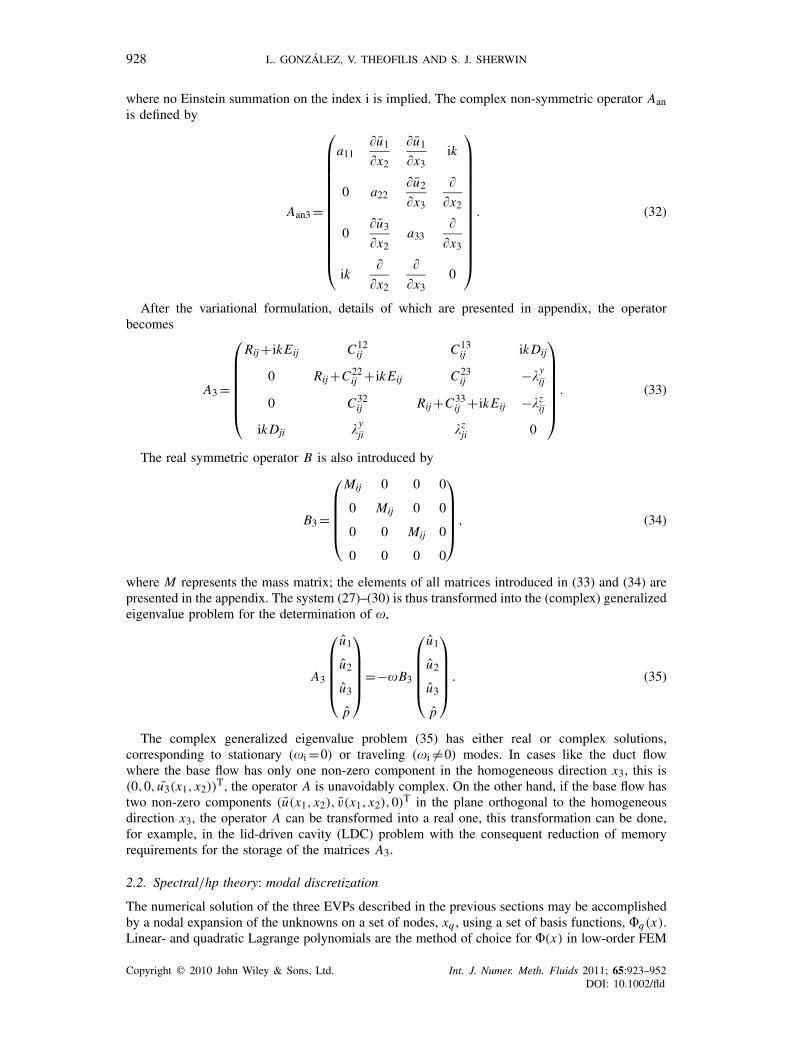
where no Einstein summation on the index i is implied. The complex non-symmetric operator Aanis defined by

Aan3=

⎛⎜⎜⎜⎜⎜⎜⎜⎜⎜⎜⎜⎜⎜⎝

a11�u1�x2

�u1�x3

ik

0 a22�u2�x3

��x2

0�u3�x2

a33�

�x3

ik�

�x2

��x3

0

⎞⎟⎟⎟⎟⎟⎟⎟⎟⎟⎟⎟⎟⎟⎠. (32)

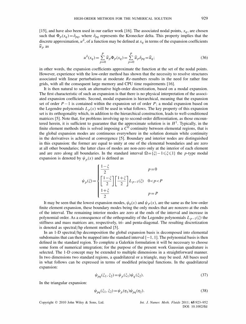
After the variational formulation, details of which are presented in appendix, the operatorbecomes

A3=

⎛⎜⎜⎜⎜⎜⎜⎝Rij+ ikEij C12

ij C13ij ikDij

0 Rij+C22ij + ikEij C23

ij −�yij

0 C32ij Rij+C33

ij + ikEij −�zij

ikDji �yji �zji 0

⎞⎟⎟⎟⎟⎟⎟⎠ . (33)


B3=

⎛⎜⎜⎜⎜⎝Mij 0 0 0

0 Mij 0 0

0 0 Mij 0

0 0 0 0

⎞⎟⎟⎟⎟⎠ , (34)

where M represents the mass matrix; the elements of all matrices introduced in (33) and (34) arepresented in the appendix. The system (27)–(30) is thus transformed into the (complex) generalizedeigenvalue problem for the determination of �,

A3

⎛⎜⎜⎜⎜⎝u1

u2

u3

p

⎞⎟⎟⎟⎟⎠=−�B3

⎛⎜⎜⎜⎜⎝u1

u2

u3

p

⎞⎟⎟⎟⎟⎠ . (35)

The complex generalized eigenvalue problem (35) has either real or complex solutions,corresponding to stationary (�i=0) or traveling (�i �=0) modes. In cases like the duct flowwhere the base flow has only one non-zero component in the homogeneous direction x3, this is(0,0, u3(x1, x2))T, the operator A is unavoidably complex. On the other hand, if the base flow hastwo non-zero components (u(x1, x2), v(x1, x2),0)T in the plane orthogonal to the homogeneousdirection x3, the operator A can be transformed into a real one, this transformation can be done,for example, in the lid-driven cavity (LDC) problem with the consequent reduction of memoryrequirements for the storage of the matrices A3.

2.2. Spectral/hp theory: modal discretizationThe numerical solution of the three EVPs described in the previous sections may be accomplishedby a nodal expansion of the unknowns on a set of nodes, xq , using a set of basis functions, �q(x).Linear- and quadratic Lagrange polynomials are the method of choice for �(x) in low-order FEM



[15], and have also been used in our earlier work [16]. The associated nodal points, xq , are chosensuch that �p(xq)=�pq, where �pq represents the Kronecker delta. This property implies that thediscrete approximation, u�, of a function may be defined at xq in terms of the expansion coefficientsu p as

u�(xq)=P∑

p=0u p�p(xq)=

P∑p=0

u p�pq= uq; (36)

in other words, the expansion coefficients approximate the function at the set of the nodal points.However, experience with the low-order method has shown that the necessity to resolve structuresassociated with linear perturbations at moderate Re-numbers results in the need for rather finegrids, with all the consequent large memory and CPU time requirements [16].

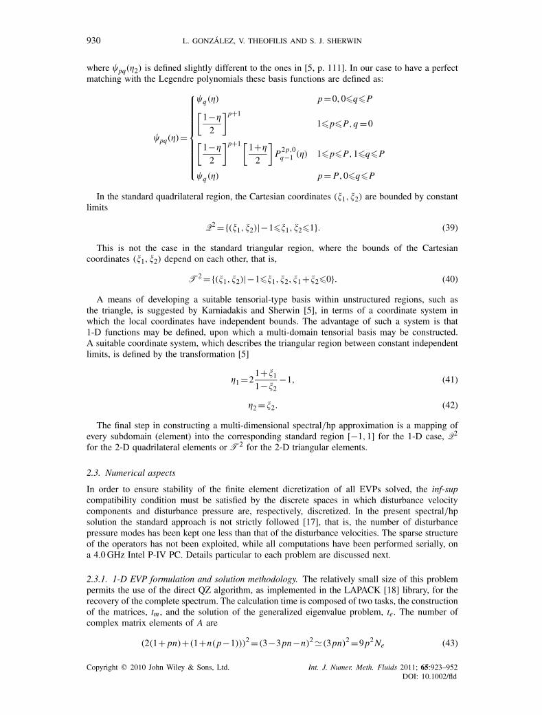
It is then natural to seek an alternative high-order discretization, based on a modal expansion.The first characteristic of such an expansion is that there is no physical interpretation of the associ-ated expansion coefficients. Second, modal expansion is hierarchical, meaning that the expansionset of order P−1 is contained within the expansion set of order P; a modal expansion based onthe Legendre polynomials L p(x) will be used in what follows. The key property of this expansionset is its orthogonality which, in addition to the hierarchical construction, leads to well-conditionedmatrices [5]. Note that, for problems involving up to second-order differentiation, as those encoun-tered herein, it is sufficient to guarantee that the approximate solution is in H1. Typically, in thefinite element methods this is solved imposing a C0 continuity between elemental regions, that isthe global expansion modes are continuous everywhere in the solution domain while continuityin the derivatives is achieved at convergence [5]. Boundary and interior nodes are distinguishedin this expansion: the former are equal to unity at one of the elemental boundaries and are zeroat all other boundaries; the latter class of modes are non-zero only at the interior of each elementand are zero along all boundaries. In the standard interval �={�|−1��1} the p-type modalexpansion is denoted by �p(x) and is defined as

�p(�)=

⎧⎪⎪⎪⎪⎪⎪⎪⎨⎪⎪⎪⎪⎪⎪⎪⎩

1−�

2p=0[

1−�

2

][1+�

2

]L p−1(�) 0<p<P

1+�

2p= P

It may be seen that the lowest expansion modes, �0(x) and �P(x), are the same as the low-orderfinite element expansion, these boundary modes being the only modes that are nonzero at the endsof the interval. The remaining interior modes are zero at the ends of the interval and increase inpolynomial order. As a consequence of the orthogonality of the Legendre polynomials L p−1(�) thestiffness and mass matrices are, respectively, tri- and penta-diagonal. The resulting discretizationis denoted as spectral/hp element method [5].

In an 1-D spectral/hp decomposition the global expansion basis is decomposed into elementalsubdomains that can then be mapped into the standard interval [−1,1]. The polynomial basis is thendefined in the standard region. To complete a Galerkin formulation it will be necessary to choosesome form of numerical integration; for the purpose of the present work Gaussian quadrature isselected. The 1-D concept may be extended to multiple dimensions in a straightforward manner.In two dimensions two standard regions, a quadrilateral or a triangle, may be used. All bases usedin what follows can be expressed in terms of modified principal functions. In the quadrilateralexpansion:

�pq(�1,�2)=�p(�1)�q(�2). (37)

In the triangular expansion:

�pq(�1,�2)=�p(1)�pq(2). (38)



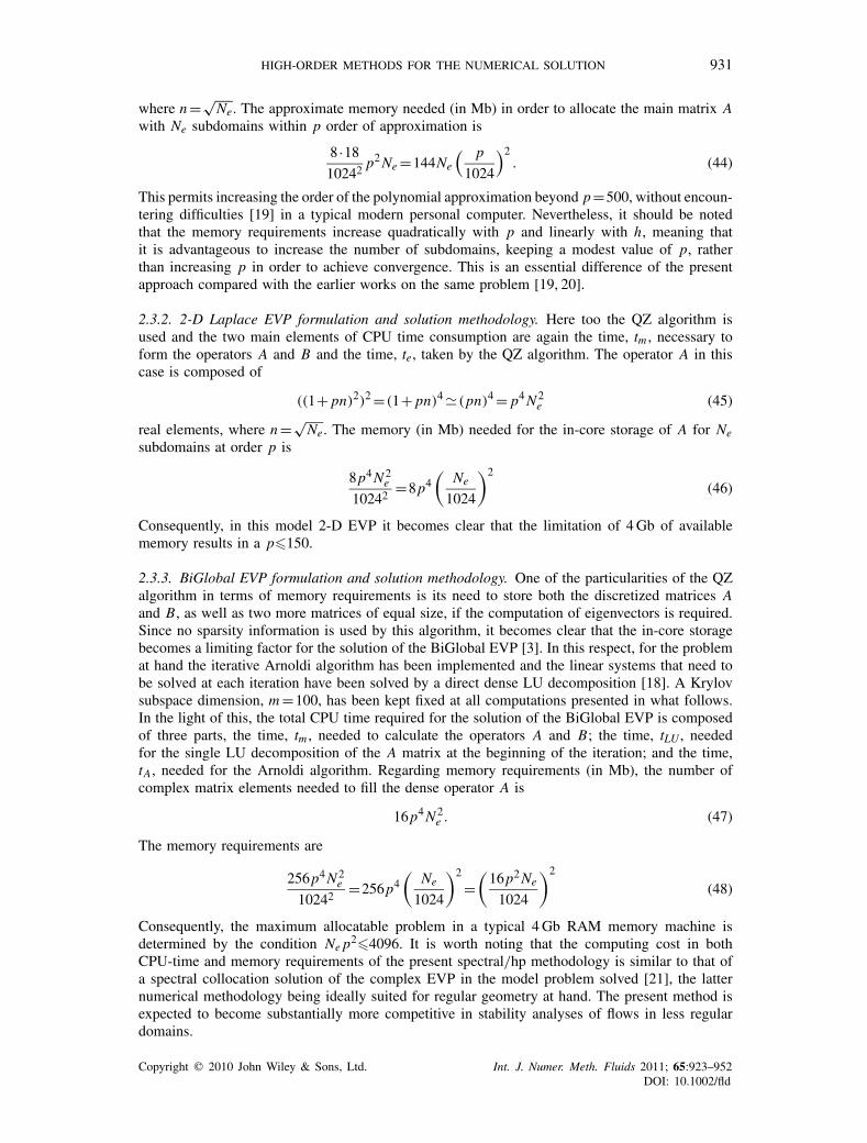
where �pq(2) is defined slightly different to the ones in [5, p. 111]. In our case to have a perfectmatching with the Legendre polynomials these basis functions are defined as:

�pq()=

⎧⎪⎪⎪⎪⎪⎪⎪⎪⎪⎨⎪⎪⎪⎪⎪⎪⎪⎪⎪⎩

�q() p=0,0�q�P[1−

2

]p+1

1�p�P,q=0[1−

2

]p+1[1+

2

]P2p,0q−1 () 1�p�P,1�q�P

�q() p= P,0�q�P

In the standard quadrilateral region, the Cartesian coordinates (�1,�2) are bounded by constantlimits

Q2={(�1,�2)|−1��1,�2�1}. (39)

This is not the case in the standard triangular region, where the bounds of the Cartesiancoordinates (�1,�2) depend on each other, that is,

T2={(�1,�2)|−1��1,�2,�1+�2�0}. (40)

A means of developing a suitable tensorial-type basis within unstructured regions, such asthe triangle, is suggested by Karniadakis and Sherwin [5], in terms of a coordinate system inwhich the local coordinates have independent bounds. The advantage of such a system is that1-D functions may be defined, upon which a multi-domain tensorial basis may be constructed.A suitable coordinate system, which describes the triangular region between constant independentlimits, is defined by the transformation [5]

1=21+�11−�2

−1, (41)

2=�2. (42)

The final step in constructing a multi-dimensional spectral/hp approximation is a mapping ofevery subdomain (element) into the corresponding standard region [−1,1] for the 1-D case, Q2

for the 2-D quadrilateral elements or T2 for the 2-D triangular elements.

2.3. Numerical aspects

In order to ensure stability of the finite element dicretization of all EVPs solved, the inf-supcompatibility condition must be satisfied by the discrete spaces in which disturbance velocitycomponents and disturbance pressure are, respectively, discretized. In the present spectral/hpsolution the standard approach is not strictly followed [17], that is, the number of disturbancepressure modes has been kept one less than that of the disturbance velocities. The sparse structureof the operators has not been exploited, while all computations have been performed serially, ona 4.0GHz Intel P-IV PC. Details particular to each problem are discussed next.

2.3.1. 1-D EVP formulation and solution methodology. The relatively small size of this problempermits the use of the direct QZ algorithm, as implemented in the LAPACK [18] library, for therecovery of the complete spectrum. The calculation time is composed of two tasks, the constructionof the matrices, tm , and the solution of the generalized eigenvalue problem, te. The number ofcomplex matrix elements of A are

(2(1+ pn)+(1+n(p−1)))2=(3−3pn−n)2�(3pn)2=9p2Ne (43)



where n=√Ne. The approximate memory needed (in Mb) in order to allocate the main matrix A

with Ne subdomains within p order of approximation is

8 ·1810242

p2Ne=144Ne

( p

1024

)2. (44)

This permits increasing the order of the polynomial approximation beyond p=500, without encoun-tering difficulties [19] in a typical modern personal computer. Nevertheless, it should be notedthat the memory requirements increase quadratically with p and linearly with h, meaning thatit is advantageous to increase the number of subdomains, keeping a modest value of p, ratherthan increasing p in order to achieve convergence. This is an essential difference of the presentapproach compared with the earlier works on the same problem [19, 20].

2.3.2. 2-D Laplace EVP formulation and solution methodology. Here too the QZ algorithm isused and the two main elements of CPU time consumption are again the time, tm , necessary toform the operators A and B and the time, te, taken by the QZ algorithm. The operator A in thiscase is composed of

((1+ pn)2)2=(1+ pn)4�(pn)4= p4N 2e (45)

real elements, where n=√Ne. The memory (in Mb) needed for the in-core storage of A for Ne

subdomains at order p is

8p4N 2e

10242=8p4

(Ne

1024

)2

(46)

Consequently, in this model 2-D EVP it becomes clear that the limitation of 4Gb of availablememory results in a p�150.

2.3.3. BiGlobal EVP formulation and solution methodology. One of the particularities of the QZalgorithm in terms of memory requirements is its need to store both the discretized matrices Aand B, as well as two more matrices of equal size, if the computation of eigenvectors is required.Since no sparsity information is used by this algorithm, it becomes clear that the in-core storagebecomes a limiting factor for the solution of the BiGlobal EVP [3]. In this respect, for the problemat hand the iterative Arnoldi algorithm has been implemented and the linear systems that need tobe solved at each iteration have been solved by a direct dense LU decomposition [18]. A Krylovsubspace dimension, m=100, has been kept fixed at all computations presented in what follows.In the light of this, the total CPU time required for the solution of the BiGlobal EVP is composedof three parts, the time, tm , needed to calculate the operators A and B; the time, tLU , neededfor the single LU decomposition of the A matrix at the beginning of the iteration; and the time,tA, needed for the Arnoldi algorithm. Regarding memory requirements (in Mb), the number ofcomplex matrix elements needed to fill the dense operator A is

16p4N 2e . (47)

The memory requirements are

256p4N 2e

10242=256p4

(Ne

1024

)2

=(16p2Ne

1024

)2

(48)

Consequently, the maximum allocatable problem in a typical 4Gb RAM memory machine isdetermined by the condition Ne p2�4096. It is worth noting that the computing cost in bothCPU-time and memory requirements of the present spectral/hp methodology is similar to that ofa spectral collocation solution of the complex EVP in the model problem solved [21], the latternumerical methodology being ideally suited for regular geometry at hand. The present method isexpected to become substantially more competitive in stability analyses of flows in less regulardomains.



3. RESULTS

Several eigenvalue problems have been solved using the methodology discussed in the previoussections. The first is the classic linear instability of plane Poiseuille flow [22], which is addressed bythe solution of the 1-D EVP in primitive-variables formulation. A model 2-D EVP with analyticallyknown solutions [14] is solved next. The next two problems address BiGlobal linear instabilityin duct flows of rectangular and triangular cross-sections; the first of these is well-documented[21, 23] while the results in the latter problem are first obtained herein. A regularized cavity flowis analyzed next by a Bi-Global linear instability considering a regularized boundary condition forthe base flow [24]. Finally, two curvilinear cross section intakes have also been solved for the firsttime, demonstrating the ability of the method to deal with non-regular geometries [25].

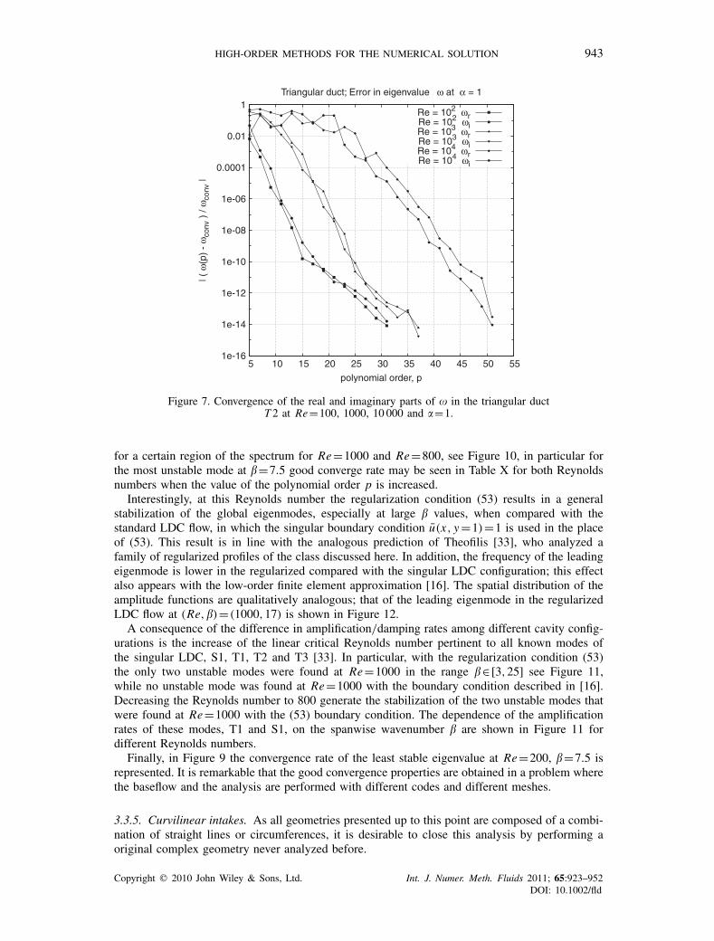
3.1. Modal linear instability in plane Poiseuille and Hagen–Poiseuille flows

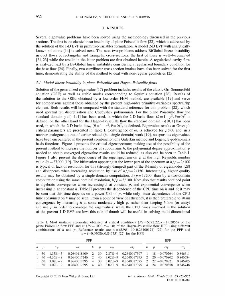
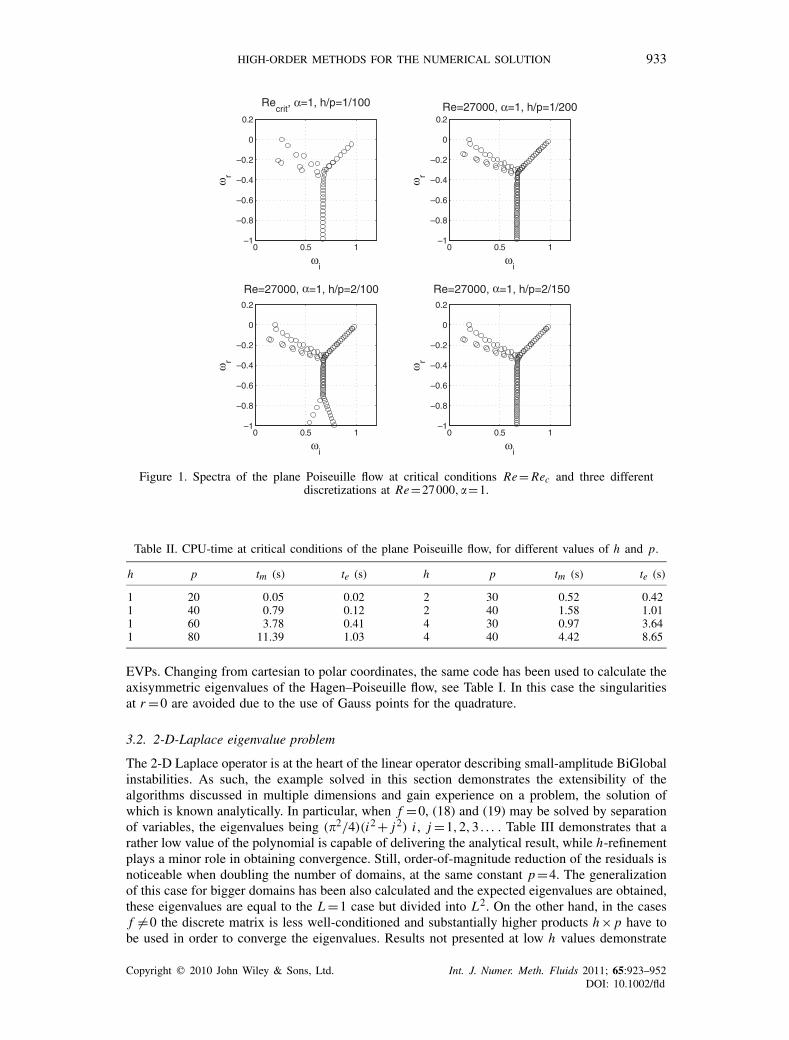
Solution of the generalized eigenvalue (17) problem includes results of the classic Orr-Sommerfeldequation (OSE) as well as stable modes corresponding to Squire’s equation [26]. Results ofthe solution to the OSE, obtained by a low-order FEM method, are available [19] and servefor comparisons against those obtained by the present high-order primitive-variables spectral/hpelement. Both results will be compared with the standard reference for this problem [22], whichused spectral tau discretization and Chebyshev polynomials. For the plane Poiseuille flow thestandard domain y∈[−1,1] has been used, in which the 2-D basic flow, (u=1− y2, v=0)T isdefined, on the other hand for the Hagen–Poiseuille flow the standard domain r ∈[0,1] has beenused, in which the 2-D basic flow, (u=1−r2, v=0)T, is defined. Eigenvalue results at Orszag’scritical parameters are presented in Table I. Convergence of �r is achieved for p�60 and, in amanner analogous to that of earlier related (but single-domain) work [19], no spurious eigenvalueshave been encountered in the present combination of a Galerkin method and Legendre-polynomialsbasis functions. Figure 1 presents the critical eigenspectrum; making use of the possibility of thepresent method to increase the number of subdomains h, the polynomial degree approximation pneeded to obtain converged eigenvalue results could be reduced, as also can be seen in Table I.Figure 1 also present the dependence of the eigenspectrum on p at the high Reynolds numbervalue Re=27000 [19]. The bifurcation appearing at the lower part of the spectrum at h/p=2/100is typical of lack of resolution for this (strongly damped) part of the S-family of eigenmodes [28]and disappears when increasing resolution by use of h/p=2/150. Interestingly, higher qualityresults may be obtained by a single-domain computation, h/p=1/200, than by a two-domaincomputation using the same nominal resolution, h/p=2/100. Note also that results obtained pointto algebraic convergence when increasing h at constant p, and exponential convergence whenincreasing p at constant h. Table II presents the dependence of the CPU time on h and p; it maybe seen that this time depends on a power l�1 of p, while only linear dependence of the CPUtime consumed on h may be seen. From a point of view of efficiency, it is then preferable to attainconvergence by increasing h at some moderately high p, rather than keeping h low (or unity)and use p in order to converge the eigenvalues; while the CPU times involved in the solutionof the present 1-D EVP are low, this rule-of-thumb will be useful in solving multi-dimensional

Table I. Most unstable eigenvalue obtained at critical conditions (Re=5772.22,�=1.02056) of theplane Poiseuille flow PPF and at (Re=1000,�=1.0) of the Hagen–Poiseuille flow HPF using differentcombinations of h and p. Reference results are �=(5.9E−10,0.26400174) [22] for the PPF and

�=(−0.07086,0.84675) [27] for the HPF.

PPF HPF

h p �r �i h p �r �i h p �r �i

1 30 1.35E−5 0.2640118409 2 30 2.87E−9 0.2640017397 1 18 −0.070764 0.8466111 40 −4.36E−8 0.2640017246 2 40 3.02E−9 0.2640017395 2 20 −0.070802 0.8466841 60 3.02E−9 0.2640017395 4 30 3.02E−9 0.2640017395 2 22 −0.070821 0.8467051 80 3.02E−9 0.2640017395 4 40 3.02E−9 0.2640017395 4 24 −0.070858 0.846748



0 0.5 1–1

–0.8

–0.6

–0.4

–0.2

0

0.2

ωi

ωr

Recrit

, α=1, h/p=1/100

0 0.5 1–1

–0.8

–0.6

–0.4

–0.2

0

0.2

ωi

ωr

Re=27000, α=1, h/p=1/200

0 0.5 1–1

–0.8

–0.6

–0.4

–0.2

0

0.2

ωi

ωr

Re=27000, α=1, h/p=2/100

0 0.5 1–1

–0.8

–0.6

–0.4

–0.2

0

0.2

ωi

ωr

Re=27000, α=1, h/p=2/150

Figure 1. Spectra of the plane Poiseuille flow at critical conditions Re= Rec and three differentdiscretizations at Re=27000,�=1.

Table II. CPU-time at critical conditions of the plane Poiseuille flow, for different values of h and p.

h p tm (s) te (s) h p tm (s) te (s)

1 20 0.05 0.02 2 30 0.52 0.421 40 0.79 0.12 2 40 1.58 1.011 60 3.78 0.41 4 30 0.97 3.641 80 11.39 1.03 4 40 4.42 8.65

EVPs. Changing from cartesian to polar coordinates, the same code has been used to calculate theaxisymmetric eigenvalues of the Hagen–Poiseuille flow, see Table I. In this case the singularitiesat r =0 are avoided due to the use of Gauss points for the quadrature.

3.2. 2-D-Laplace eigenvalue problem

The 2-D Laplace operator is at the heart of the linear operator describing small-amplitude BiGlobalinstabilities. As such, the example solved in this section demonstrates the extensibility of thealgorithms discussed in multiple dimensions and gain experience on a problem, the solution ofwhich is known analytically. In particular, when f =0, (18) and (19) may be solved by separationof variables, the eigenvalues being (�2/4)(i2+ j2) i , j =1,2,3 . . . . Table III demonstrates that arather low value of the polynomial is capable of delivering the analytical result, while h-refinementplays a minor role in obtaining convergence. Still, order-of-magnitude reduction of the residuals isnoticeable when doubling the number of domains, at the same constant p=4. The generalizationof this case for bigger domains has been also calculated and the expected eigenvalues are obtained,these eigenvalues are equal to the L=1 case but divided into L2. On the other hand, in the casesf �=0 the discrete matrix is less well-conditioned and substantially higher products h× p have tobe used in order to converge the eigenvalues. Results not presented at low h values demonstrate



Table III. Convergence history of the Laplace EVP, for two different forcing functions andseveral combinations of h and p.

h p �r h p �r h p �r

f =01 2 2.0264236728 2 2 2.0150446547 4 2 2.00102428101 4 2.0000294277 2 4 2.0000027311 4 4 2.00000001121 6 2.0000000068 2 6 2.0000000000 4 6 2.00000000001 8 2.0000000000 2 8 1.9999999999 4 8 2.0000000000

f =exp(20(y−x−1))1 2 137.81737070 2 2 2.4515999319 4 2 2.15120624711 4 2.2629988052 2 4 2.1484629835 4 4 2.11768389031 6 2.1627748728 2 6 2.1247358185 4 6 2.11627280161 8 2.1350717525 2 8 2.1180407896 4 8 2.11619280051 10 2.1233966472 2 10 2.1167590461 4 10 2.1161849315

Figure 2. First four eigenvectors of (18)–(19) for f (x, y)=exp[20(y−x−1)] [14].that, increasing p at constant h delivers convergence. However, (46) shows that increasing p isless efficient in terms of memory requirements and associated CPU time demands than increasingh, the dependence of the memory on p being quartic and that on h being quadratic. As such,it is preferable to seek converged results by increasing h at a moderate p. Contour plots of thefirst four eigenvectors of the f �=0 problem are shown in Figure 2; Table IV discusses that thecomputational times are measured versus h and p.

3.3. The BiGlobal instability analyses

3.3.1. Hagen–Poiseuille flow. For this case and the following the variables will be renamed.(x1, x2, x3)=(y, z, x), k=�, (u1, u2, u3)=(v, w, u). The algorithms exposed have been applied tostudy the stability of the classic Hagen Poiseuille flow (HPF). While, from a physical point ofview, this is probably the most prominent example of failure of modal linear theory to predicttransition, the corresponding 1-D eigenvalue problem (of the Orr-Sommerfeld class) has beenstudied exhaustively over the years [27, 29], thus serving for the present validation work. Theanalytically known basic flow, u=1−r2, has been recovered on the same unstructured mesh asthat on which the BiGlobal instability analysis has been performed. Results on the eigenvaluesof the two least-damped eigenmodes presented by Lessen [29] and Salwen [27] at four Reynoldsnumbers are shown in Table V, where excellent agreement with those results may be seen. The



Table IV. CPU time for different combinations of h and p.

h p tm (s) te (s)

1 4 1.2E−2 0.0001 8 0.42 2.8E−22 4 3.2E−2 2.8E−22 8 1.66 1.784 4 0.11 1.924 8 6.54 111.12

Table V. Two least-damped eigenmodes of Hagen–Poiseuille flow (HPF) at k=�=1 for different Reynoldsnumbers, obtained on an single element mesh h=1 and p polynomial degree.

Re Frequency Damping rate Frequency Damping rate

100 0.57256 −0.14714 0.55198 −0.37446 Salwen [27]100 0.57256 −0.14714 0.55198 −0.37446 Lessen [29]100 0.57256 −0.14714 0.55198 −0.37446 Present (h=1, p=18)

200 0.64427 −0.12921 0.51116 −0.20266 Salwen [27]200 0.64426 −0.12920 0.51117 −0.20265 Lessen [29]200 0.64526 −0.12920 0.51117 −0.20265 Present(h=1, p=20)



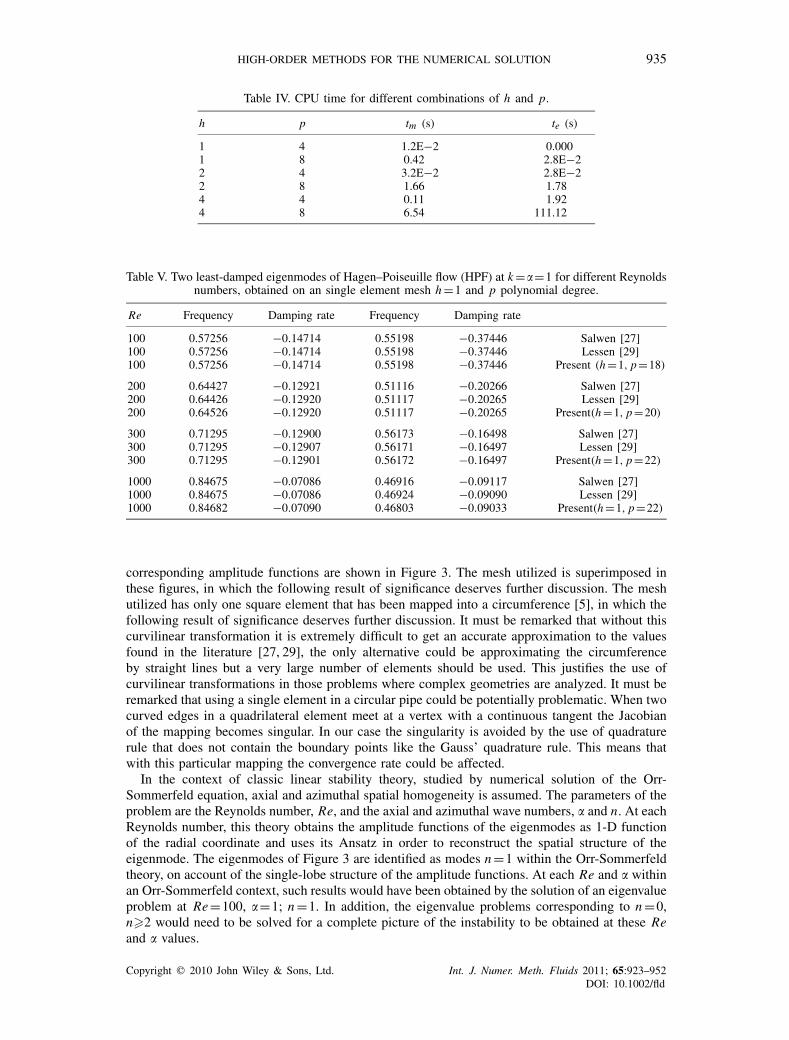
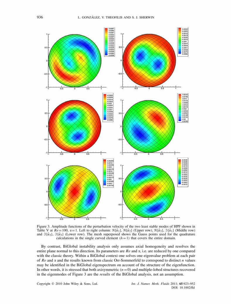
corresponding amplitude functions are shown in Figure 3. The mesh utilized is superimposed inthese figures, in which the following result of significance deserves further discussion. The meshutilized has only one square element that has been mapped into a circumference [5], in which thefollowing result of significance deserves further discussion. It must be remarked that without thiscurvilinear transformation it is extremely difficult to get an accurate approximation to the valuesfound in the literature [27, 29], the only alternative could be approximating the circumferenceby straight lines but a very large number of elements should be used. This justifies the use ofcurvilinear transformations in those problems where complex geometries are analyzed. It must beremarked that using a single element in a circular pipe could be potentially problematic. When twocurved edges in a quadrilateral element meet at a vertex with a continuous tangent the Jacobianof the mapping becomes singular. In our case the singularity is avoided by the use of quadraturerule that does not contain the boundary points like the Gauss’ quadrature rule. This means thatwith this particular mapping the convergence rate could be affected.

In the context of classic linear stability theory, studied by numerical solution of the Orr-Sommerfeld equation, axial and azimuthal spatial homogeneity is assumed. The parameters of theproblem are the Reynolds number, Re, and the axial and azimuthal wave numbers, � and n. At eachReynolds number, this theory obtains the amplitude functions of the eigenmodes as 1-D functionof the radial coordinate and uses its Ansatz in order to reconstruct the spatial structure of theeigenmode. The eigenmodes of Figure 3 are identified as modes n=1 within the Orr-Sommerfeldtheory, on account of the single-lobe structure of the amplitude functions. At each Re and � withinan Orr-Sommerfeld context, such results would have been obtained by the solution of an eigenvalueproblem at Re=100, �=1; n=1. In addition, the eigenvalue problems corresponding to n=0,n�2 would need to be solved for a complete picture of the instability to be obtained at these Reand � values.



Figure 3. Amplitude functions of the perturbation velocity of the two least stable modes of HPF shown inTable V at Re=100, �=1. Left to right column: {u1}, {u2} (Upper row), {u3}, {u1} (Middle row)and {u2}, {u3} (Lower row). The mesh superposed shows the Gauss points used for the quadrature

calculations in the single curved element (h=1) that covers the entire domain.

By contrast, BiGlobal instability analysis only assumes axial homogeneity and resolves theentire plane normal to this direction. Its parameters are Re and �, i.e. are reduced by one comparedwith the classic theory. Within a BiGlobal context one solves one eigenvalue problem at each pairof Re and � and the results known from classic Orr-Sommerfeld to correspond to distinct n valuesmay be identified in the BiGlobal eigenspectrum on account of the structure of the eigenfunction.In other words, it is stressed that both axisymmetric (n=0) and multiple-lobed structures recoveredin the eigenmodes of Figure 3 are the results of the BiGlobal analysis, not an assumption.



3.3.2. Rectangular duct flow. Turning to the rectangular duct problem, the stability of which wasfirst solved by Tatsumi and Yoshimura [23] is now going to be analyzed by the present method.Although spectral collocation would be an obvious option in order to discretize the spatial operator,in this case many other possibilities are available if spectral elements are used. A single elementwith increasing polynomial order has been used for the first convergence analysis, also othercentered quadrilateral meshes and even hybrid meshes have been used for both the basic flowcalculations and the instability analyses. The existence of a steady basic state implies stability ofthe 2-D (�=0) eigenmodes, such that the objective of the analysis becomes interrogation of theflow with respect to its stability to 3-D (� �=0) small-amplitude perturbations. Unlike the seminalwork of Tatsumi and Yoshimura [23] on this problem the symmetries of the basic state havenot been exploited in the instability analysis. The complex EVP to be solved here is (35), forwhich no reduction to a real problem is possible. The single component of the basic flow velocityvector, (0,0, u(y, z)), is obtained from numerical solution (also using an spectral/hp elementdiscretization) of the Poisson problem

∇2u(x, y)=−2, (49)

u|�b =0; (50)

the maximum value of the basic state obtained has been used to normalize u. Note thatusing the meshes necessary for convergence of the instability analysis results, the numericallyobtained solution is identical with the (also numerically obtained) analytical solution of (49), see[30]

u(x, y)= 1− y2

2− 16

�3∞∑

k=1,k odd

sin[k�(1+ y)/2]

k3 sinhk�

{sinh

[k�(1+x)

2

]+sinh

[k�(1−x)

2

]}. (51)

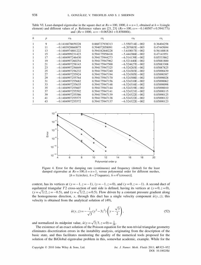
To confirm the spectral convergence of the method a single element mesh was studied fordifferent polynomial order approximations at different Reynolds numbers. Results are presented inTable VI where the good convergence properties can be appreciated. In this case the base flow wascalculated analytically by the expression (51). Error analysis of the damping rate and frequencyresults, using the values provided by a well-validated spectral collocation code [21] as a reference,show that convergence of the leading eigenvalue is obtained at a moderate polynomial order,p=14, and the relative error of the eigenvalue obtained compared with the spectral collocationresult [21] of the same cEVP is of O(10−6). Results displayed in Figure 4 demonstrate exponentialconvergence.

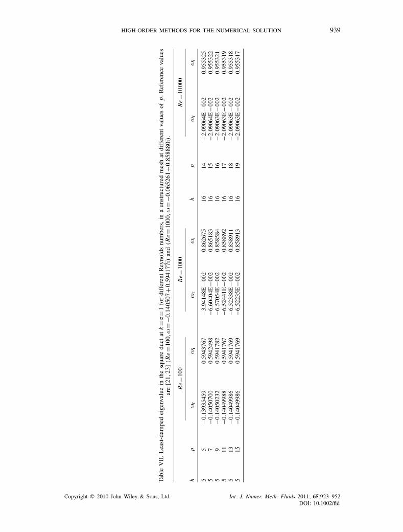
A similar instability analysis have been repeated with an unstructured mesh using a baseflowcoming from the solution of (49) in the square duct at Re=100,1000, 10 000, results are presentedin Table VII where good accuracy has been obtained for the leading eigenmode increasing the pvalue and keeping h with a constant value. Finally, the computational solution in the general hybridmesh described above has been also performed. The amplitude function of the leading dampedeigenmode at Re=100,�=1 can be seen in Figure 5.

In Table IX computational times are measured versus h and p.In this case the only geometrical degree of freedom that is present is the possibility of changing

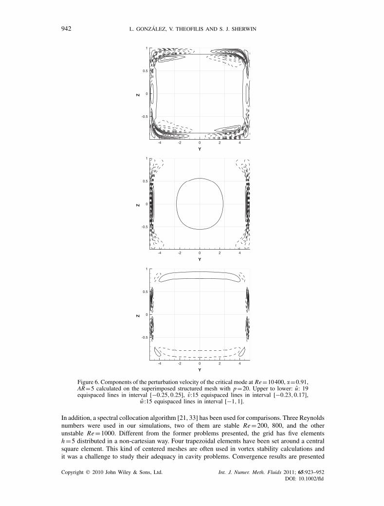
the aspect ratio AR, one of the critical points studied by [21, 23] has also been calculated,that is Re=10400, �=0.91, AR=5. The mesh used for the calculation is a 16(4×4) elementstructured mesh with four elements per row and column. Calculations were done for two differentpolynomial approximations, obtaining for p=18 a imaginary part �i=0.2126994i and for p=20�i=0.2115566i, where good agreement can be appreciated [21] �i=0.21167i. The eigenvectorcorresponding to the critical mode is also shown in Figure 6.

The situation as far as the efficiency of the numerical approach is concerned changes as theReynolds number increases. It is known that increasingly larger grids will be necessary in orderto resolve the increasingly finer structures appearing as Re increases.

3.3.3. Triangular duct flow. Two different triangular cross-section geometries have been analyzed.The first triangular duct T 1, which can be named as the canonical triangle in the spectral element



Table VI. Least-damped eigenvalue in the square duct at Re=100,1000, k=�=1, obtained at h=1(singleelement) and different values of p. Reference values are [21, 23] (Re=100,�=−0.140507+0.594177i)

and (Re=1000, �=−0.065261+0.858880i).

h p �r �i �r �i

1 9 −0.1416878659228 0.868727938313 −3.550714E−002 0.364042581 11 −0.1403920660875 0.594072058091 −6.207683E−003 0.474456941 13 −0.1404974881222 0.594182840228 −3.610017E−002 0.561488181 15 −0.1404999231423 0.594175958418 −5.444386E−002 0.471419511 17 −0.1404997246430 0.594175944273 −6.514139E−002 0.855338621 19 −0.1404997260254 0.594175947962 −6.521440E−002 0.858818001 21 −0.1404997258143 0.594175947500 −6.524627E−002 0.858833081 23 −0.1404997256849 0.594175947325 −6.524283E−002 0.858878251 25 −0.1404997256232 0.594175947240 −6.524303E−002 0.858904391 27 −0.1404997255924 0.594175947194 −6.524305E−002 0.858903871 29 −0.1404997255764 0.594175947170 −6.524308E−002 0.858900281 31 −0.1404997255682 0.594175947156 −6.524310E−002 0.858900621 33 −0.1404997255635 0.594175947148 −6.524316E−002 0.858900981 35 −0.1404997255607 0.594175947144 −6.524319E−002 0.858900101 37 −0.1404997255592 0.594175947141 −6.524321E−002 0.858901151 39 −0.1404997255586 0.594175947139 −6.524322E−002 0.858901251 41 −0.1404997255575 0.594175947138 −6.524322E−002 0.858901221 43 −0.1404997255572 0.594175947137 −6.524322E−002 0.85890123

Figure 4. Error for the damping rate (continuous) and frequency (dotted) for the leastdamped eigenvalue at Re=100,k=�=1, versus polynomial order for different meshes,

[h=1(circles), h=22(squares), h=42(crosses)].

context, has its vertices at (y=−1, z=−1), (y=−1, z=0), and (y=0, z=−1). A second duct ofequilateral triangular T 2 cross-section of unit side is defined, having its vertices at (y=0, z=0),(y=√

3/2, z=−0.5), and (y=√3/2, z=0.5). Flow driven by a constant pressure gradient along

the homogeneous direction, x , through this duct has a single velocity component u(y, z); thisvelocity is obtained from the analytical solution of (49),

u(y, z)=− 1√3(y2−3z2)

(y−

√3

2

), (52)

and normalized its midpoint value, u(y=√3/3, z=0)= 1

18 .The existence of an exact solution of the Poisson equation for the non-trivial triangular geometry

eliminates discretization errors in the instability analysis, originating from the description of thebasic state, and thus facilitates monitoring the quality of the numerical tools proposed for thesolution of the BiGlobal eigenvalue problem in this, somewhat academic, example. While for the



TableVII.Least-dam

pedeigenvalue

inthesquare

duct

atk=�

=1fordifferentReynoldsnumbers,in

aunstructured

meshat

differentvalues

ofp.

Reference

values

are

[21,23]

(Re=1

00,�

=−0.140507

+0.594177i

)and

(Re=1

000,

�=−

0.065261

+0.858880i

).

Re=1

00Re=1

000

Re=1

000

0

hp

�r

�i

�r

�i

hp

�r

�i

55

−0.139

3545

90.59

4376

7−3

.941

48E

−002

0.86

2675

1614

−2.090

64E

−002

0.95

5325

57

−0.140

5070

00.59

4249

8−6

.604

04E

−002

0.86

5183

1615

−2.090

64E

−002

0.95

5322

59

−0.140

5023

20.59

4178

2−6

.570

54E

−002

0.85

8584

1616

−2.090

63E

−002

0.95

5321

511

−0.140

4998

80.59

4176

7−6

.524

41E

−002

0.85

8892

1617

−2.090

63E

−002

0.95

5319

513

−0.140

4998

60.59

4176

9−6

.523

38E

−002

0.85

8911

1618

−2.090

63E

−002

0.95

5318

515

−0.140

4998

60.59

4176

9−6

.522

35E

−002

0.85

8913

1619

−2.090

63E

−002

0.95

5317



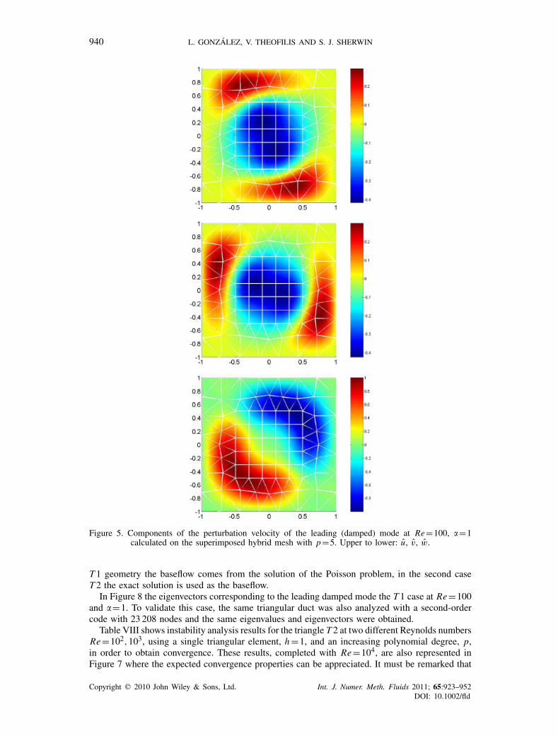
Figure 5. Components of the perturbation velocity of the leading (damped) mode at Re=100, �=1calculated on the superimposed hybrid mesh with p=5. Upper to lower: u, v, w.

T 1 geometry the baseflow comes from the solution of the Poisson problem, in the second caseT 2 the exact solution is used as the baseflow.

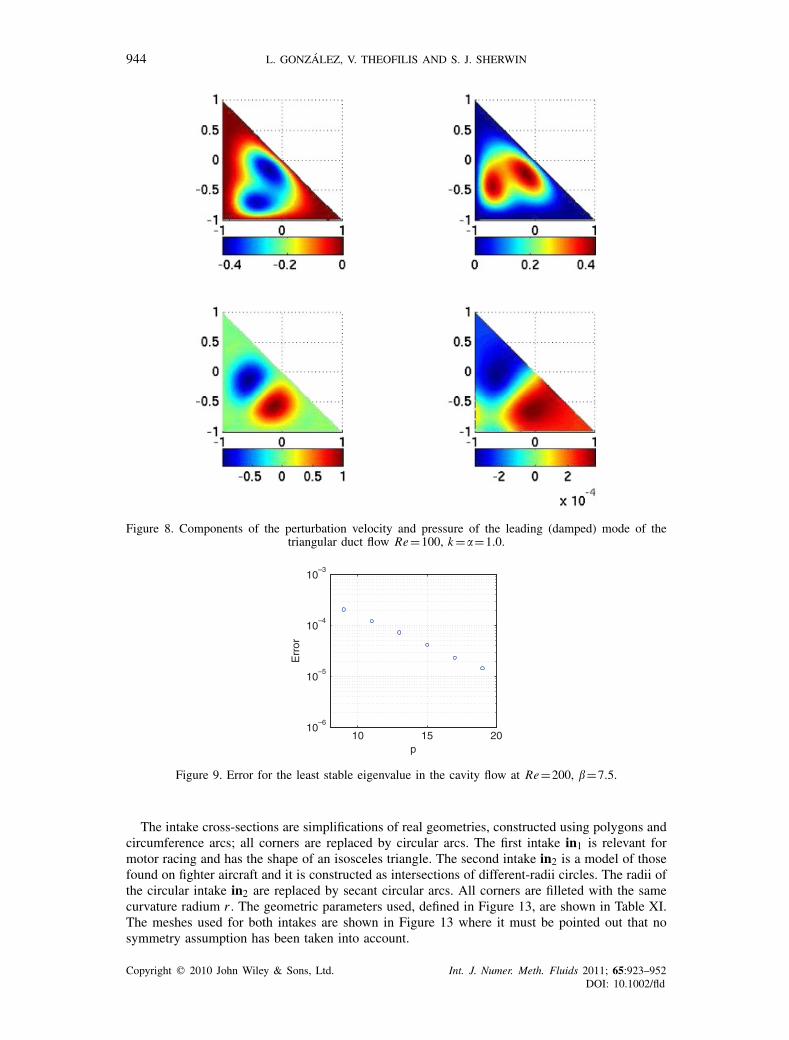
In Figure 8 the eigenvectors corresponding to the leading damped mode the T 1 case at Re=100and �=1. To validate this case, the same triangular duct was also analyzed with a second-ordercode with 23 208 nodes and the same eigenvalues and eigenvectors were obtained.

Table VIII shows instability analysis results for the triangle T 2 at two different Reynolds numbersRe=102,103, using a single triangular element, h=1, and an increasing polynomial degree, p,in order to obtain convergence. These results, completed with Re=104, are also represented inFigure 7 where the expected convergence properties can be appreciated. It must be remarked that



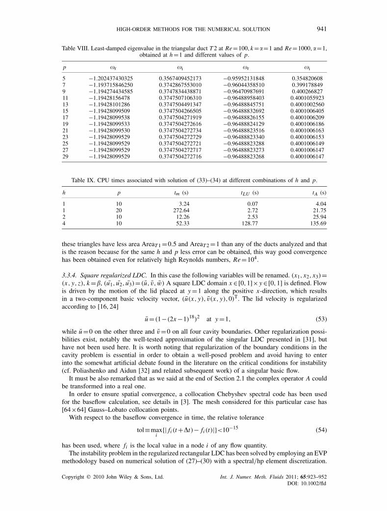
Table VIII. Least-damped eigenvalue in the triangular duct T 2 at Re=100,k=�=1 and Re=1000,�=1,obtained at h=1 and different values of p.

p �r �i �r �i

5 −1.202437430325 0.3567409452173 −0.95952131848 0.3548206087 −1.193715846250 0.3742867553010 −0.96044358510 0.3991788499 −1.194274434585 0.3747834438871 −0.96470987691 0.40026682711 −1.19428156478 0.3747507106310 −0.96488958403 0.400105592313 −1.19428101286 0.3747504491347 −0.96488845751 0.400100256015 −1.19428099509 0.3747504266505 −0.96488832692 0.400100640517 −1.19428099538 0.3747504271919 −0.96488826155 0.400100620919 −1.19428099533 0.3747504272616 −0.96488824129 0.400100618621 −1.19428099530 0.3747504272734 −0.96488823516 0.400100616323 −1.19428099529 0.3747504272729 −0.96488823340 0.400100615325 −1.19428099529 0.3747504272721 −0.96488823288 0.400100614927 −1.19428099529 0.3747504272717 −0.96488823273 0.400100614729 −1.19428099529 0.3747504272716 −0.96488823268 0.4001006147

Table IX. CPU times associated with solution of (33)–(34) at different combinations of h and p.

h p tm (s) tLU (s) tA (s)

1 10 3.24 0.07 4.041 20 272.64 2.72 21.752 10 12.26 2.53 25.944 10 52.33 128.77 135.69

these triangles have less area AreaT 1=0.5 and AreaT 2=1 than any of the ducts analyzed and thatis the reason because for the same h and p less error can be obtained, this way good convergencehas been obtained even for relatively high Reynolds numbers, Re=104.

3.3.4. Square regularized LDC. In this case the following variables will be renamed. (x1, x2, x3)=(x, y, z), k=, (u1, u2, u3)=(u, v, w) A square LDC domain x ∈[0,1]× y∈[0,1] is defined. Flowis driven by the motion of the lid placed at y=1 along the positive x-direction, which resultsin a two-component basic velocity vector, (u(x, y), v(x, y),0)T. The lid velocity is regularizedaccording to [16, 24]

u=(1−(2x−1)18)2 at y=1, (53)

while u=0 on the other three and v=0 on all four cavity boundaries. Other regularization possi-bilities exist, notably the well-tested approximation of the singular LDC presented in [31], buthave not been used here. It is worth noting that regularization of the boundary conditions in thecavity problem is essential in order to obtain a well-posed problem and avoid having to enterinto the somewhat artificial debate found in the literature on the critical conditions for instability(cf. Poliashenko and Aidun [32] and related subsequent work) of a singular basic flow.

It must be also remarked that as we said at the end of Section 2.1 the complex operator A couldbe transformed into a real one.

In order to ensure spatial convergence, a collocation Chebyshev spectral code has been usedfor the baseflow calculation, see details in [3]. The mesh considered for this particular case has[64×64] Gauss–Lobato collocation points.

With respect to the baseflow convergence in time, the relative tolerance

tol≡maxi

{| fi (t+�t)− fi (t)|}<10−15 (54)

has been used, where fi is the local value in a node i of any flow quantity.The instability problem in the regularized rectangular LDC has been solved by employing an EVP

methodology based on numerical solution of (27)–(30) with a spectral/hp element discretization.



Y

Z-4 -2 0 2 4

-0.5

0

0.5

1

Y

Z

-4 -2 0 2 4

-0.5

0

0.5

1

Y

Z

-4 -2 0 2 4

-0.5

0

0.5

1

Figure 6. Components of the perturbation velocity of the critical mode at Re=10400, �=0.91,AR=5 calculated on the superimposed structured mesh with p=20. Upper to lower: u: 19equispaced lines in interval [−0.25,0.25], v:15 equispaced lines in interval [−0.23,0.17],

w:15 equispaced lines in interval [−1,1].

In addition, a spectral collocation algorithm [21, 33] has been used for comparisons. Three Reynoldsnumbers were used in our simulations, two of them are stable Re=200, 800, and the otherunstable Re=1000. Different from the former problems presented, the grid has five elementsh=5 distributed in a non-cartesian way. Four trapezoidal elements have been set around a centralsquare element. This kind of centered meshes are often used in vortex stability calculations andit was a challenge to study their adequacy in cavity problems. Convergence results are presented



1e-16

1e-14

1e-12

1e-10

1e-08

1e-06

0.0001

0.01

1

5 10 15 20 25 30 35 40 45 50 55

| ( ω

(p)

- ω

conv

) /

ωco

nv |

polynomial order, p

Triangular duct; Error in eigenvalue ω at α = 1

Re = 102 ωrRe = 102 ωiRe = 103 ωrRe = 103 ωiRe = 104 ωrRe = 104 ωi

Figure 7. Convergence of the real and imaginary parts of � in the triangular ductT 2 at Re=100, 1000, 10 000 and �=1.

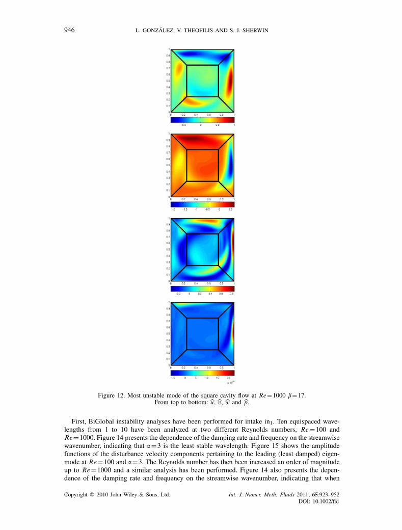
for a certain region of the spectrum for Re=1000 and Re=800, see Figure 10, in particular forthe most unstable mode at =7.5 good converge rate may be seen in Table X for both Reynoldsnumbers when the value of the polynomial order p is increased.

Interestingly, at this Reynolds number the regularization condition (53) results in a generalstabilization of the global eigenmodes, especially at large values, when compared with thestandard LDC flow, in which the singular boundary condition u(x, y=1)=1 is used in the placeof (53). This result is in line with the analogous prediction of Theofilis [33], who analyzed afamily of regularized profiles of the class discussed here. In addition, the frequency of the leadingeigenmode is lower in the regularized compared with the singular LDC configuration; this effectalso appears with the low-order finite element approximation [16]. The spatial distribution of theamplitude functions are qualitatively analogous; that of the leading eigenmode in the regularizedLDC flow at (Re,)=(1000,17) is shown in Figure 12.

A consequence of the difference in amplification/damping rates among different cavity config-urations is the increase of the linear critical Reynolds number pertinent to all known modes ofthe singular LDC, S1, T1, T2 and T3 [33]. In particular, with the regularization condition (53)the only two unstable modes were found at Re=1000 in the range ∈[3,25] see Figure 11,while no unstable mode was found at Re=1000 with the boundary condition described in [16].Decreasing the Reynolds number to 800 generate the stabilization of the two unstable modes thatwere found at Re=1000 with the (53) boundary condition. The dependence of the amplificationrates of these modes, T1 and S1, on the spanwise wavenumber are shown in Figure 11 fordifferent Reynolds numbers.

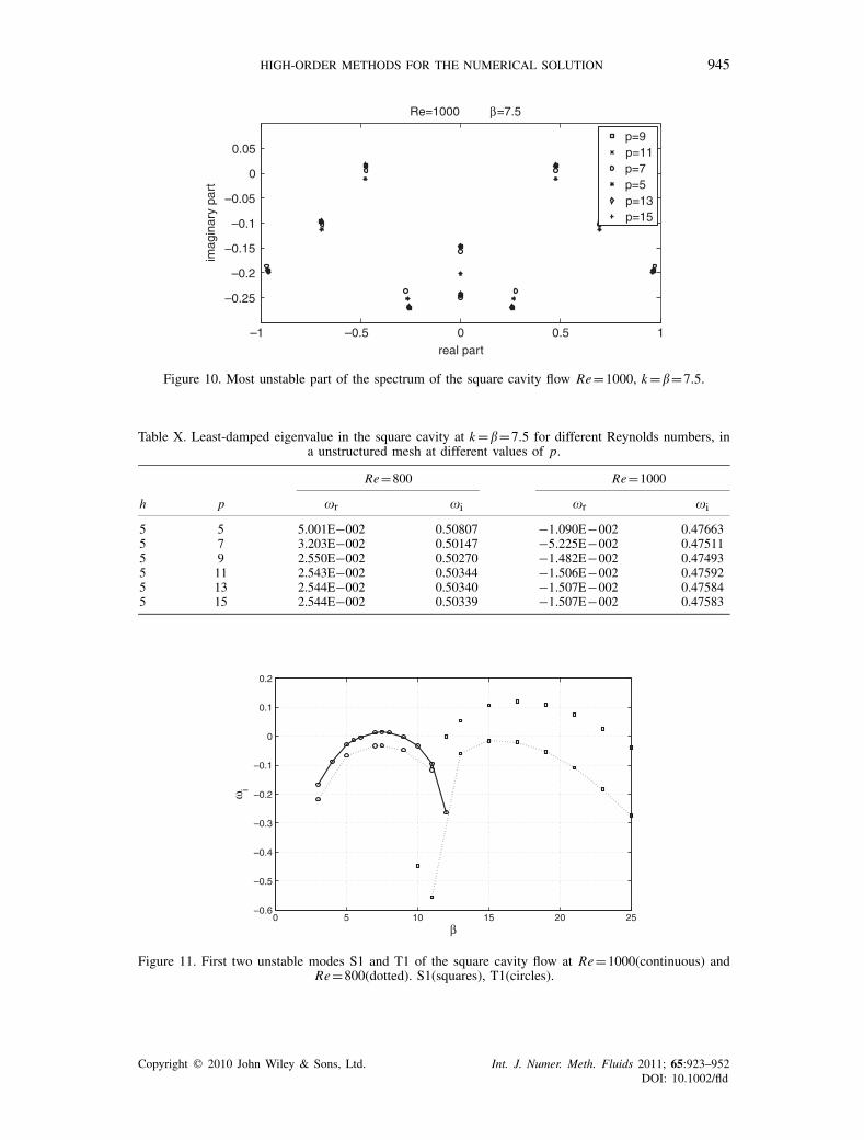
Finally, in Figure 9 the convergence rate of the least stable eigenvalue at Re=200, =7.5 isrepresented. It is remarkable that the good convergence properties are obtained in a problem wherethe baseflow and the analysis are performed with different codes and different meshes.

3.3.5. Curvilinear intakes. As all geometries presented up to this point are composed of a combi-nation of straight lines or circumferences, it is desirable to close this analysis by performing aoriginal complex geometry never analyzed before.



Figure 8. Components of the perturbation velocity and pressure of the leading (damped) mode of thetriangular duct flow Re=100, k=�=1.0.

10 15 2010

–6

10–5

10–4

10–3

p

Err

or

Figure 9. Error for the least stable eigenvalue in the cavity flow at Re=200, =7.5.

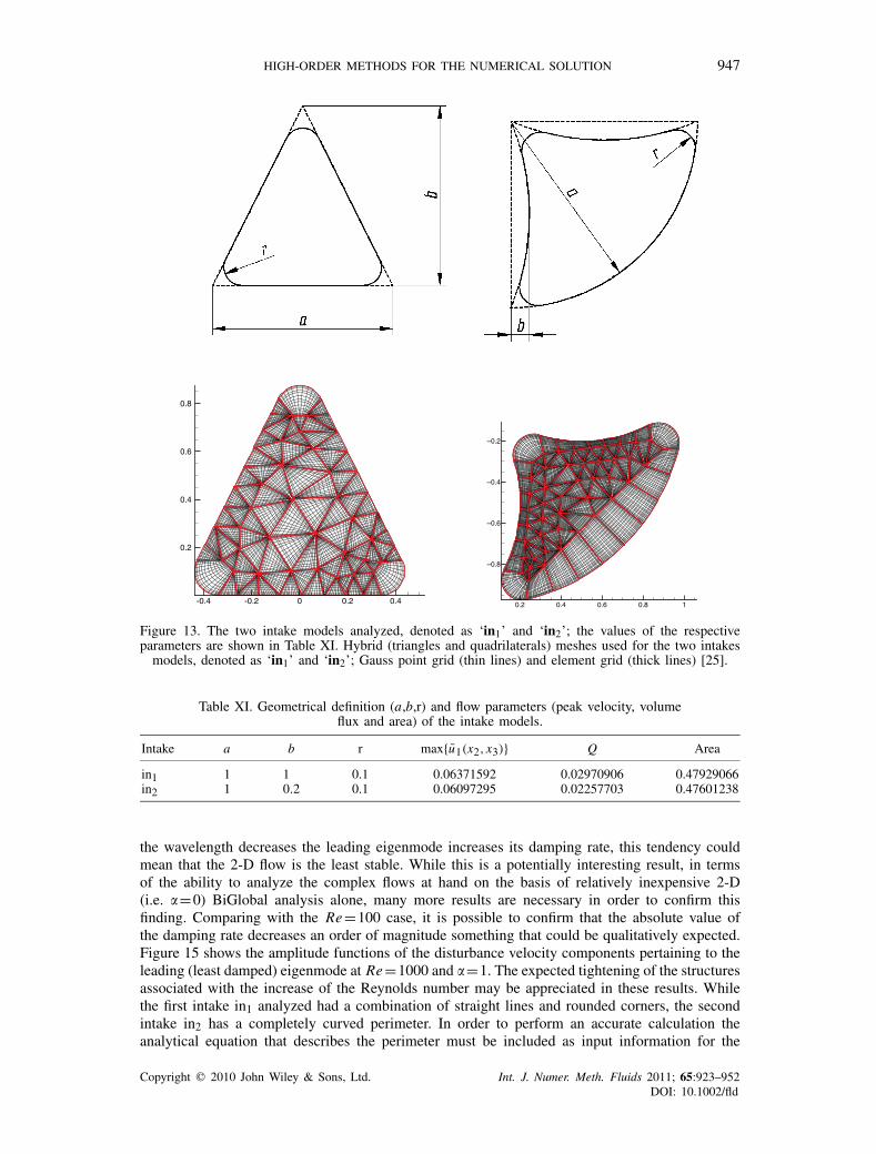
The intake cross-sections are simplifications of real geometries, constructed using polygons andcircumference arcs; all corners are replaced by circular arcs. The first intake in1 is relevant formotor racing and has the shape of an isosceles triangle. The second intake in2 is a model of thosefound on fighter aircraft and it is constructed as intersections of different-radii circles. The radii ofthe circular intake in2 are replaced by secant circular arcs. All corners are filleted with the samecurvature radium r . The geometric parameters used, defined in Figure 13, are shown in Table XI.The meshes used for both intakes are shown in Figure 13 where it must be pointed out that nosymmetry assumption has been taken into account.



–1 –0.5 0 0.5 1

–0.25

–0.2

–0.15

–0.1

–0.05

0

0.05

real part

imag

inar

y pa

rt

Re=1000 β=7.5

p=9p=11p=7p=5p=13p=15

Figure 10. Most unstable part of the spectrum of the square cavity flow Re=1000, k==7.5.

Table X. Least-damped eigenvalue in the square cavity at k==7.5 for different Reynolds numbers, ina unstructured mesh at different values of p.

Re=800 Re=1000

h p �r �i �r �i

5 5 5.001E−002 0.50807 −1.090E−002 0.476635 7 3.203E−002 0.50147 −5.225E−002 0.475115 9 2.550E−002 0.50270 −1.482E−002 0.474935 11 2.543E−002 0.50344 −1.506E−002 0.475925 13 2.544E−002 0.50340 −1.507E−002 0.475845 15 2.544E−002 0.50339 −1.507E−002 0.47583

0 5 10 15 20 25–0.6

–0.5

–0.4

–0.3

–0.2

–0.1

0

0.1

0.2

β

ωi

Figure 11. First two unstable modes S1 and T1 of the square cavity flow at Re=1000(continuous) andRe=800(dotted). S1(squares), T1(circles).



Figure 12. Most unstable mode of the square cavity flow at Re=1000 =17.From top to bottom: u, v, w and p.

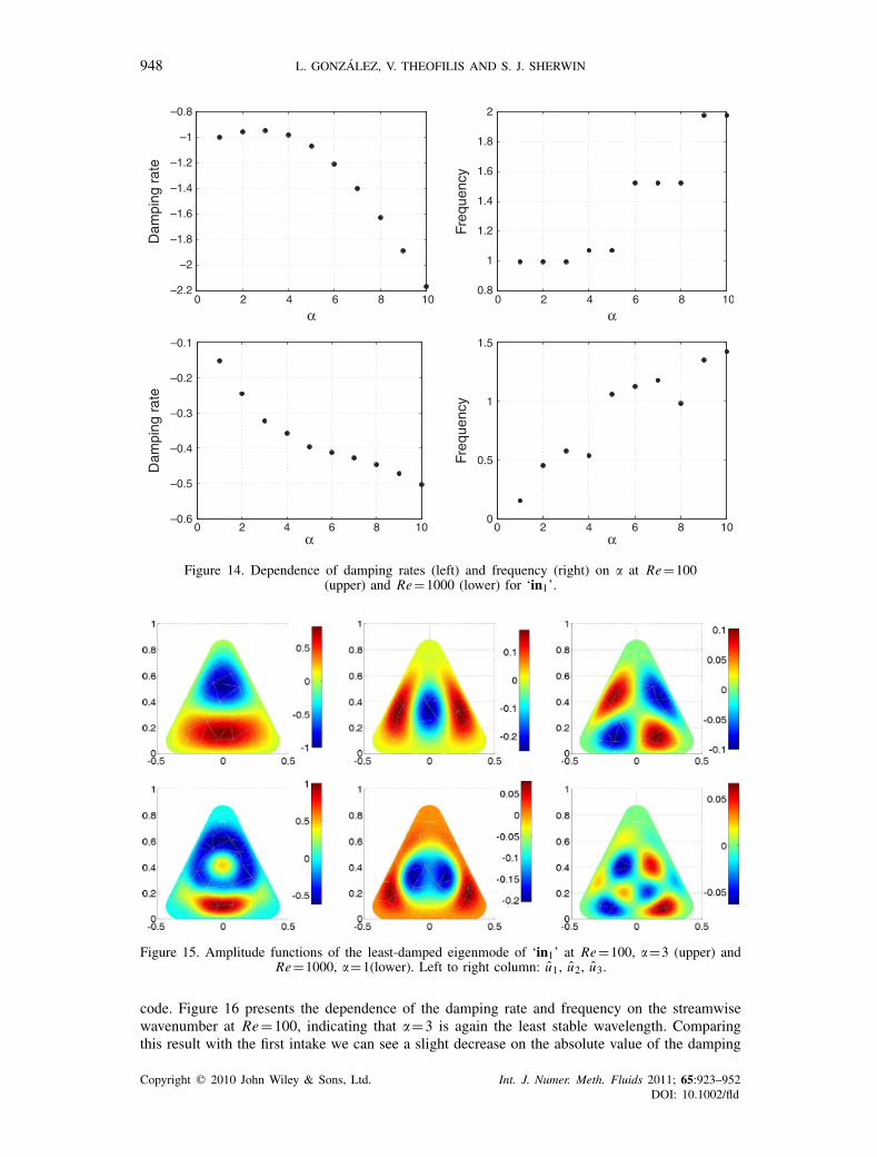
First, BiGlobal instability analyses have been performed for intake in1. Ten equispaced wave-lengths from 1 to 10 have been analyzed at two different Reynolds numbers, Re=100 andRe=1000. Figure 14 presents the dependence of the damping rate and frequency on the streamwisewavenumber, indicating that �=3 is the least stable wavelength. Figure 15 shows the amplitudefunctions of the disturbance velocity components pertaining to the leading (least damped) eigen-mode at Re=100 and �=3. The Reynolds number has then been increased an order of magnitudeup to Re=1000 and a similar analysis has been performed. Figure 14 also presents the depen-dence of the damping rate and frequency on the streamwise wavenumber, indicating that when



-0.4 -0.2 0 0.2 0.4

0.2

0.4

0.6

0.8

0.2 0.4 0.6 0.8 1

–0.8

–0.6

–0.4

–0.2

Figure 13. The two intake models analyzed, denoted as ‘in1’ and ‘in2’; the values of the respectiveparameters are shown in Table XI. Hybrid (triangles and quadrilaterals) meshes used for the two intakesmodels, denoted as ‘in1’ and ‘in2’; Gauss point grid (thin lines) and element grid (thick lines) [25].

Table XI. Geometrical definition (a,b,r) and flow parameters (peak velocity, volumeflux and area) of the intake models.

Intake a b r max{u1(x2, x3)} Q Area

in1 1 1 0.1 0.06371592 0.02970906 0.47929066in2 1 0.2 0.1 0.06097295 0.02257703 0.47601238

the wavelength decreases the leading eigenmode increases its damping rate, this tendency couldmean that the 2-D flow is the least stable. While this is a potentially interesting result, in termsof the ability to analyze the complex flows at hand on the basis of relatively inexpensive 2-D(i.e. �=0) BiGlobal analysis alone, many more results are necessary in order to confirm thisfinding. Comparing with the Re=100 case, it is possible to confirm that the absolute value ofthe damping rate decreases an order of magnitude something that could be qualitatively expected.Figure 15 shows the amplitude functions of the disturbance velocity components pertaining to theleading (least damped) eigenmode at Re=1000 and �=1. The expected tightening of the structuresassociated with the increase of the Reynolds number may be appreciated in these results. Whilethe first intake in1 analyzed had a combination of straight lines and rounded corners, the secondintake in2 has a completely curved perimeter. In order to perform an accurate calculation theanalytical equation that describes the perimeter must be included as input information for the



0 2 4 6 8 10–2.2

–2

–1.8

–1.6

–1.4

–1.2

–1

–0.8

α

Dam

ping

rat

e

0 2 4 6 8 100.8

1

1.2

1.4

1.6

1.8

2

α

Freq

uenc

y

0 2 4 6 8 10–0.6

–0.5

–0.4

–0.3

–0.2

–0.1

α

Dam

ping

rat

e

0 2 4 6 8 100

0.5

1

1.5

α

Freq

uenc

y

Figure 14. Dependence of damping rates (left) and frequency (right) on � at Re=100(upper) and Re=1000 (lower) for ‘in1’.

Figure 15. Amplitude functions of the least-damped eigenmode of ‘in1’ at Re=100, �=3 (upper) andRe=1000, �=1(lower). Left to right column: u1, u2, u3.

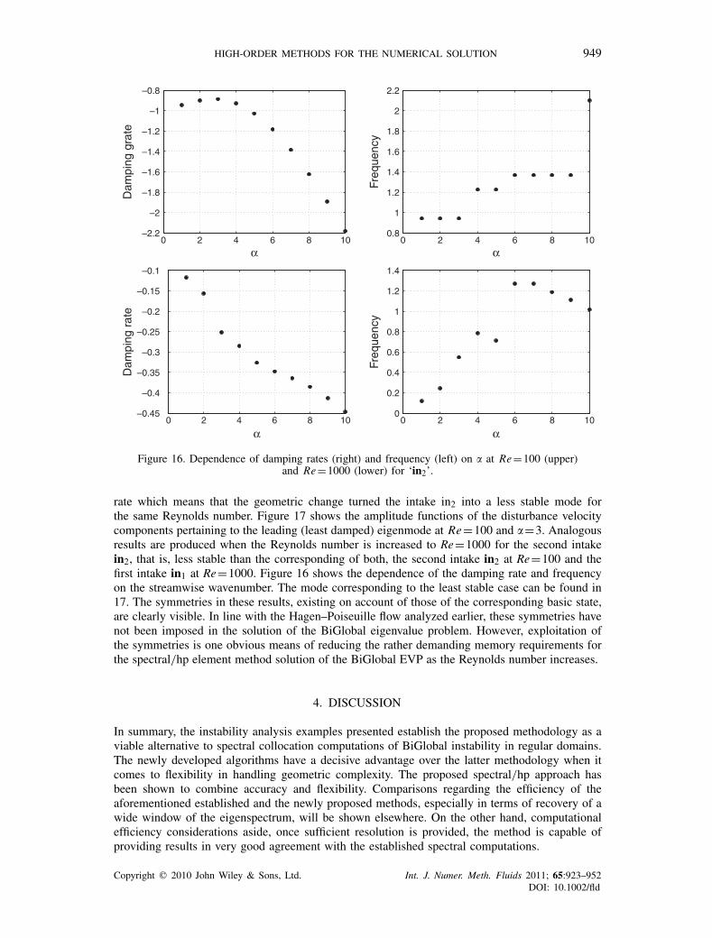
code. Figure 16 presents the dependence of the damping rate and frequency on the streamwisewavenumber at Re=100, indicating that �=3 is again the least stable wavelength. Comparingthis result with the first intake we can see a slight decrease on the absolute value of the damping



0 2 4 6 8 10–2.2

–2

–1.8

–1.6

–1.4

–1.2

–1

–0.8

α

Dam

ping

gra

te

0 2 4 6 8 100.8

1

1.2

1.4

1.6

1.8

2

2.2

α

Freq

uenc

y

0 2 4 6 8 10–0.45

–0.4

–0.35

–0.3

–0.25

–0.2

–0.15

–0.1

α

Dam

ping

rat

e

0 2 4 6 8 100

0.2

0.4

0.6

0.8

1

1.2

1.4

α

Freq

uenc

y

Figure 16. Dependence of damping rates (right) and frequency (left) on � at Re=100 (upper)and Re=1000 (lower) for ‘in2’.

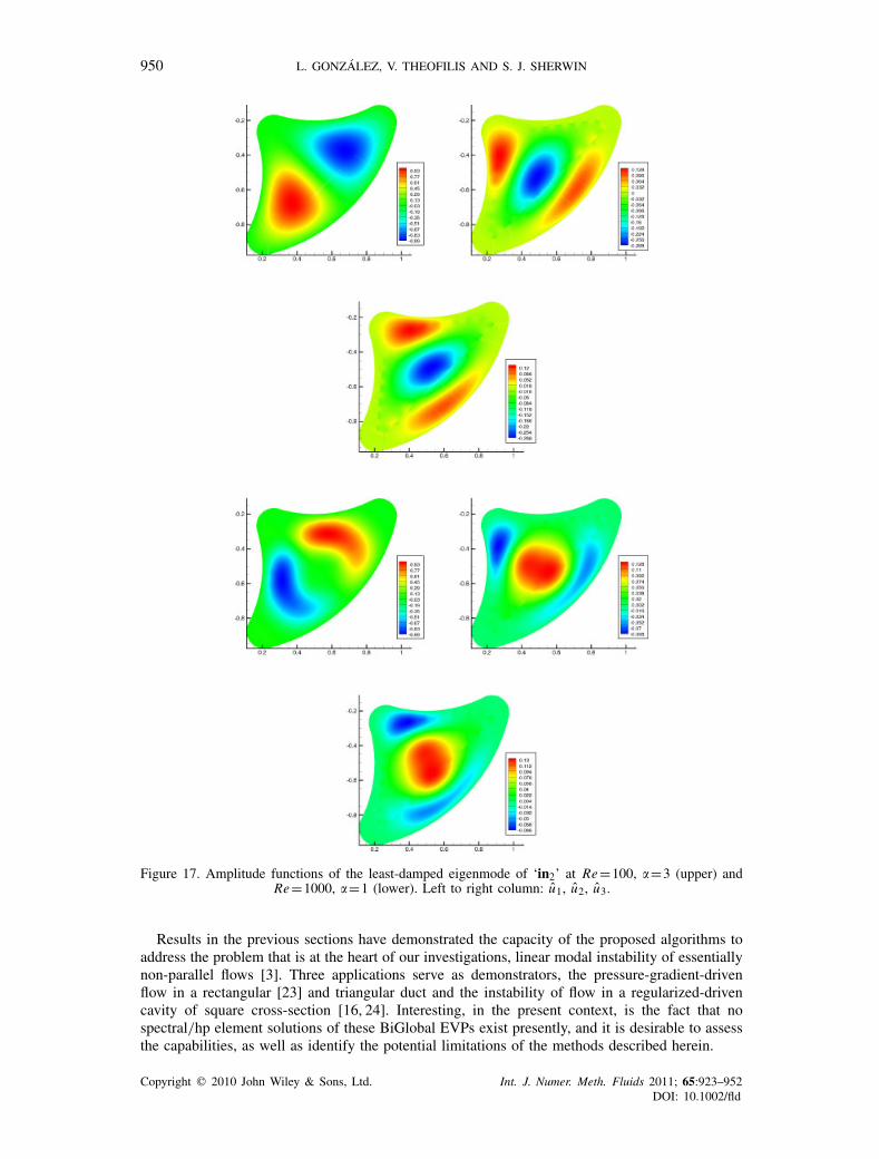
rate which means that the geometric change turned the intake in2 into a less stable mode forthe same Reynolds number. Figure 17 shows the amplitude functions of the disturbance velocitycomponents pertaining to the leading (least damped) eigenmode at Re=100 and �=3. Analogousresults are produced when the Reynolds number is increased to Re=1000 for the second intakein2, that is, less stable than the corresponding of both, the second intake in2 at Re=100 and thefirst intake in1 at Re=1000. Figure 16 shows the dependence of the damping rate and frequencyon the streamwise wavenumber. The mode corresponding to the least stable case can be found in17. The symmetries in these results, existing on account of those of the corresponding basic state,are clearly visible. In line with the Hagen–Poiseuille flow analyzed earlier, these symmetries havenot been imposed in the solution of the BiGlobal eigenvalue problem. However, exploitation ofthe symmetries is one obvious means of reducing the rather demanding memory requirements forthe spectral/hp element method solution of the BiGlobal EVP as the Reynolds number increases.

4. DISCUSSION

In summary, the instability analysis examples presented establish the proposed methodology as aviable alternative to spectral collocation computations of BiGlobal instability in regular domains.The newly developed algorithms have a decisive advantage over the latter methodology when itcomes to flexibility in handling geometric complexity. The proposed spectral/hp approach hasbeen shown to combine accuracy and flexibility. Comparisons regarding the efficiency of theaforementioned established and the newly proposed methods, especially in terms of recovery of awide window of the eigenspectrum, will be shown elsewhere. On the other hand, computationalefficiency considerations aside, once sufficient resolution is provided, the method is capable ofproviding results in very good agreement with the established spectral computations.



Figure 17. Amplitude functions of the least-damped eigenmode of ‘in2’ at Re=100, �=3 (upper) andRe=1000, �=1 (lower). Left to right column: u1, u2, u3.

Results in the previous sections have demonstrated the capacity of the proposed algorithms toaddress the problem that is at the heart of our investigations, linear modal instability of essentiallynon-parallel flows [3]. Three applications serve as demonstrators, the pressure-gradient-drivenflow in a rectangular [23] and triangular duct and the instability of flow in a regularized-drivencavity of square cross-section [16, 24]. Interesting, in the present context, is the fact that nospectral/hp element solutions of these BiGlobal EVPs exist presently, and it is desirable to assessthe capabilities, as well as identify the potential limitations of the methods described herein.



Based on the numerical experimentation presented we observe that the suite of spectral element-based algorithms discussed is capable of delivering accurate predictions for the complex BiGlobalEVP at Reynolds numbers of typical relevance to instability analysis. Nevertheless, the questionwhether the proposed store-and-invert methodology is a viable alternative to the computationallyefficient time-stepping approaches [7] still need be addressed in future studies.

APPENDIX A: DETAILS OF THE GALERKIN FORMULATION

Defining the velocity basis functions as � and the pressure basis functions as �, the followingentries of the matrices A and B (for each element) in the different eigenvalue problems appearingin Equations (15), (22) and (33) are obtained

Rij=∫

�

��i

�xm

�� j

�xmd�, i, j =1, . . . , P+1 m=1,2. (A1)

Mij=∫

��i� jd�, i, j =1, . . . , P+1. (A2)

Eij=∫

�u1�i� j d�, i, j =1, . . . , P+1. (A3)

Ckmij =

∫�

(�uk�xm

)�i� j d�, i, j =1, . . . , P+1 k=1,2,3 m=1,2. (A4)

Dij=∫

��i� j d�, i=1, . . . , P j =1, . . . , P+1 (A5)

�yij=∫

��i

�� j

�yd�, i=1, . . . , P j =1, . . . , P+1. (A6)

Fij=∫

�f (x, y)�i� j d�, i, j =1, . . . , P+1. (A7)

ACKNOWLEDGEMENTS

This work has been supported by a grant of the Universidad Politecnica de Madrid which make possiblea short stay of Dr.Gonzalez at the Imperial College London. The authors also wish to acknowledge theColegio-Asociacion de Ingenieros del ICAI for the funding and support of this research. Thanks are dueto Mr. D. Rodrıguez for his contribution in the mathematical description of the curvilinear intakes.

REFERENCES

1. Peyret R. Spectral Methods for Incompressible Viscous Flow. Springer: Berlin, 2002.2. Canuto C, Hussaini M, Quarteroni A, Zang T. Spectral Methods in Fluid Dynamics. Springer: Berlin, 1987.3. Theofilis V. Advances in global linear instability analysis of nonparallel and three-dimensional flows. Progress

in Aerospace Sciences 2003; 39:249–315.4. Barkley D, Blackburn HM, Sherwin SJ. Direct optimal growth analysis for timesteppers. International Journal

for Numerical Methods in Fluids 2008; 57:1435–1458.5. Karniadakis GE, Sherwin SJ. Spectral/hp Element Methods for Computational Fluid Dynamics (2nd edn). Oxford

University Press: Oxford, 2005.6. Barkley D, Henderson RD. Three-dimensional floquet stability analysis of the wake of a circular cylinder. Journal

of Fluid Mechanics 1996; 322:215–241.7. Tuckerman L, Barkley D. Bifurcation Analysis for Timesteppers. IMA Volumes in Mathematics and its

Applications. Springer: New York, 1999; 453–466.8. Edwards WS, Tuckerman LS, Friesner RA, Sorensen DC. Krylov methods for the incompressible Navier–Stokes

equations. Journal of Computational Physics 1994; 110(1):82–102.9. Theofilis V, Barkley D, Sherwin SJ. Spectral/hp element technology for flow instability and control. Aeronautical

Journal 2002; 106:619–625.



10. Sherwin SJ, Blackburn HM. Three-dimensional instabilities of steady and pulsatile axisymmetric stenotic flows.Journal of Fluid Mechanics 2005; 533:297–327.

11. Abdessemed N, Sherwin SJ, Theofilis V. Linear instability analysis of low pressure turbine flows. Journal ofFluid Mechanics 2009; 628:57–83.

12. Fietier N, Deville M. Time-dependent algorithms for the simulation of viscoelastic flows with spectral elementmethods: applications and stability. Journal of Computational Physics 2003; 186:93–121.

13. Kitsios V, Rodriguez D, Theofilis V, Ooi Soria J. Biglobal instability analysis of turbulent flow over an airfoil atan angle of attack. Thirty-eighth Fluid Dynamics Conference and Exhibit, Seattle, Washington, 2008; 9. AIAA,

no. Paper 2008-2541.14. Trefethen L. Spectral Methods in Matlab. SIAM: Philadelphia, 2000.15. Cuvelier C, Segal A, van Steenhoven AA. Finite Element Methods and Navier-Stokes Equations. D. Reidel

Publishing Company: Dordrecht, 1986.16. Gonzalez L, Theofilis V, Gomez-Blanco R. Finite-element numerical methods for viscous incompressible biglobal

linear instability analysis on unstructured meshes. AIAA Journal 2007; 45(4):840–855.17. Maday CBY. Approximations Spectrales de Problemes Aux Limites Elliptiques. Springer: Paris, 1992.18. Anderson E, Bai Z, Bischof C, Blackford S, Demmel J, Dongarra J, Du Croz J, Greenbaum A, Hammarling S,

McKenney A, Sorensen D. LAPACK Users’ Guide (3rd edn). Society for Industrial and Applied Mathematics:Philadelphia, PA, 1999.

19. Kirchner N. Computational aspects of the spectral Galerkin fem for the Orr-Sommerfeld equation. InternationalJournal for Numerical Methods in Fluids 2000; 32:119–137.

20. Schwab C. p and hp-Finite Element Methods. Theory and Applications in Solid and Fluid Mechanics. OxfordScience Publications: Oxford, U.K., 2004.

21. Theofilis V, Duck PW, Owen J. Viscous linear stability analysis of rectangular duct and cavity flows. Journal ofFluid Mechanics 2004; 505:249–286.

22. Orszag S. Accurate solution of the orr-sommerfeld stability equation. Journal of Fluid Mechanics 1971; 50:689–703.

23. Tatsumi T, Yoshimura T. Stability of the laminar flow in a rectangular duct. Journal of Fluid Mechanics 1990;212:437–449.

24. Leriche E, Gavrilakis S, Deville MO. Direct simulation of the lid-driven cavity flow with chebyshev polynomials.In Proceedings of the 4th European Computational Fluid Dynamics Conference (ECCOMAS), Papailiou KD(ed.), Athens, Greece, vol. 1(1), 1998; 220–225.

25. Gonzalez L, Rodriguez D, Theofilis V. On instability analysis of realistic intake flows. Thirty-seventh AIAA FluidDynamics Conference, Seattle, WA, 23–26 Jun 2008; 9. AIAA no. Paper 2004-4380.

26. Schmid P, Henningson DS. Stability and Transition in Shear Flows. Springer: New York, 2001.27. Salwen H, Cotton FW, Grosch CE. Linear stability of poiseuille flow in a circular pipe. Journal of Fluid

Mechanics 1980; 98:273–284.28. Jimenez J. A numerical study of the temporal eigenvalue spectrum of the Blasius boundary layer. Journal of

Fluid Mechanics 1976; 73:497–520.29. Lessen M, Sadler SG, Liu TY. Stability of pipe poiseuille flow. Physics of Fluids 1968; 11:1404–1409.30. Rosenhead L. Laminar Boundary Layers. Oxford University Press: Oxford, 1963.31. Bourcier M, Francois C. Integration numerique des equations de Navier–Stokes dans un domine carre. La

Recherche Aerospatiale 1969; 131:23–33.32. Poliashenko M, Aidun CK. A direct method for computation of simple bifurcations. Journal of Computational

Physics 1995; 121:246–260.33. Theofilis V. Globally unstable basic flows in open cavities. AIAA 2000; 2000–1965:12.


Documents

High-order methods for the numerical solution of the BiGlobal linear stability eigenvalue problem in complex geometries