Embed Size (px)
Citation preview

By Facundo Alvaredo and Juliana Londoño Vélez
HIGH INCOMES AND PERSONAL TAXATION IN A DEVELOPING ECONOMY: COLOMBIA 1993-2010
Working Paper No. 12
March 2013

2
High Incomes and Personal Taxation in a Developing Economy: Colombia 1993-2010
Facundo Alvaredo
Nuffield/EMod-Oxford, Paris School of Economics, Conicet
Juliana Londoño Vélez Paris School of Economics, Ministry of Finance and Public Credit, Colombia1
CEQ Working Paper
19 March 2013
ABSTRACT We present series of the shares of income accruing to the top groups of the distribution in Colombia between 1993 and 2010, based on individual income tax data. We obtain four main empirical results. First, income in Colombia is highly concentrated, the top 1% of the income distribution accounting for over 20% of total income in 2010. This is at the highest level of inequality in any recent year in the entire WTID sample. Second, high-income individuals in Colombia are, in essence, rentiers and capital owners. Third, while households’ surveys show that inequality has been decreasing since 2006, tax-based results offer a different picture, where concentration at the top has remained stable; when survey based Gini coefficients are adjusted to take into account higher incomes reported to tax files, inequality levels are higher, and the recent reduction in inequality is less pronounced. Fourth, income taxation does little to reduce the high levels of inequality. Keywords: income distribution, inequality, personal income tax, Latin America JEL Codes: D31, H24, O54
1 We are particularly grateful to Anthony B. Atkinson, Isabelle Joumard, María Ana Lugo, Nora Lustig, and Thomas Piketty
for valuable comments and suggestions. The income tax data were obtained thanks to a collaborative project between DIAN and OECD. Juan Ricardo Ortega, Pastor Sierra, Natasha Avendaño, Natalia Aristizábal, Javier Ávila, and Sebastián Nieto answered to our numerous questions regarding the income tax administration. Leonardo Gasparini kindly provided results based on household surveys from SEDLAC. Carlos Chaparro helped considerably in understanding the Colombian tax code. We acknowledge financial support from ESRC, CIPR and INET. Facundo Alvaredo: [email protected]; Juliana Londoño Vélez: [email protected].

3
1. INTRODUCTION
There has been much recent interest in falling income inequality in Latin America over the past decade.
Scholars have been trying to understand such decline in a region historically characterised by high,
persistent inequality (Lustig and López Calva, 2010). However, little has been said about the very top
of the distribution. To the extent that the overwhelming majority of the literature uses households
survey data, which underestimate income concentration, a reassessment of the evolution of income
distribution is in order. In this paper we study the shares of top incomes in Colombia between 1993
and 2010 using tax data. The case of Colombia is worth studying on several grounds.
First, Colombia is the first country in Latin America to provide micro-data from the personal income
tax for a relatively long period of time (1993-2010).2 These data allow for a detailed analysis of high
incomes, including the years for which surveys indicate a decline in inequality. They also provide the
necessary information to accurately determine the average tax rates effectively paid by top income
recipients. This is a first-order concern in a continent marked by regressive tax systems.
Second, Colombia has traditionally been identified as having one of the highest Gini coefficients in
Latin America (Ferreira and Ravallion, 2008). In the beginning of the 1990s, the country embarked on
a process of market liberalization in the context of the Washington Consensus, and experienced
positive growth until 1994. Between 1994 and 2003, it plunged into the most severe economic
recession in the last century, the income per adult dropping by 13% (see Figure 1). This was followed
by an economic boom in the mid-2000s that was only temporarily interrupted by the global economic
crisis in 2008–2009. Hence, it is important to re-assess the link between growth and distribution.
Third, Colombia has undergone key changes in the political arena since the 1990s. The 1991
constitution established progressiveness as the foundation of the tax system (article 363). As a result, all
the subsequent tax reforms have been presented as serving such principle. This study can shed some
light on the extent to which these well-intentioned political efforts actually translated into real impacts
on the distribution through the tax system.
The use of tax statistics is not without drawbacks. First, since only a fraction of the population files a
tax return, studies using tax data are restricted to measuring top shares, which are silent about changes
in the lower and middle part of the distribution. Second, estimates may be biased due to tax avoidance
and tax evasion. These elements, which are common to all countries, become critical in the developing
world. In Colombia, until recently plagued by high insecurity, the rich and wealthy may be particularly
dissuaded from disclosing their fortunes and incomes to authorities, lest the information revealed fall
into the wrong hands. Indeed, anecdotal evidence suggests that, during the intense political violence of
the 1990s, leaked personal tax returns were used by criminal groups to target victims and kidnap for
ransom.
2 There are few studies on the evolution of income inequality in Colombia from a historical perspective; Londoño (1995) is an exception, as well as Londoño Vélez’ master thesis (2012), which started the work with the databases used in this paper.

4
This study obtains four main empirical results. First, income in Colombia is highly concentrated, as the
top 1% of the income distribution accounts for 20.4% of total gross income in 2010. Top income
shares are at the highest level in any recent year in the entire WTID sample, except for the US, which
has overtaken Colombia for several years in the late 1990s and the 2000s. The net-of-tax top 1% share
is 20.1% in 2010, which can be compared with the figure from the household survey: 13.5%.
Second, high-income individuals in Colombia are, in essence, rentiers and capital owners. This feature
differs from the pattern found in several developed countries in recent decades, where it has been
shown that the large increase in the share of income going to the top groups has been mainly due to
spectacular increases in executive compensation and high salaries, and to a lesser extent to a partial
restoration of capital incomes. While the working rich have joined capital owners at the top of the
income hierarchy in the United States and other English-speaking countries, Colombia remains a more
traditional society where the top income recipients are still the owners of the capital stock.
Third, while households’ surveys show that inequality measured by the Gini coefficient went down
when 2006 and 2010 are compared, tax-based results offer a different picture, in which concentration
at the top has remained stable over the same period. When survey based Gini coefficients are adjusted
to take into account top incomes reported in tax files, inequality levels are higher than previously
measured, and the recent reduction in inequality is less pronounced.
Fourth, personal taxation does little to reduce inequality. The income tax burden is very low at the
FIGURE 1
Average Real Income and Consumer Price Index in Colombia, 1990-2010
Source: Table A1.
Notes: Figure reports the average real income per adult (aged 20 and above), expressed in real 2010 thousand Colombian Pesos.
CPI index is equal to 100 in 2010.
1 USD ≈ 2,000 Colombian Pesos (2010 prices)
1
10
100
9.500
10.000
10.500
11.000
11.500
12.000
12.500
19
90
19
91
19
92
19
93
19
94
19
95
19
96
19
97
19
98
19
99
20
00
20
01
20
02
20
03
20
04
20
05
20
06
20
07
20
08
20
09
20
10
Co
ns
um
er
Pri
ce
In
de
x (
ba
se
10
0 i
n 2
01
0)
Re
al In
co
me
pe
r a
du
lt (2
01
0 th
ou
sa
nd
Co
lom
bia
n
pe
so
s)
Income control per adult
CPI

5
upper end of the income distribution, due to a multiplicity of legal tax reliefs, even without considering
the effects of evasion.
These results are not a novelty from the qualitative point of view, in the light of the well-known high
inequality levels and distortive tax systems in Latin America. However, they challenge the general
scepticism regarding the use of tax data from developing countries to study inequality. Our estimates
should be regarded as a lower bound, to take into account the effects of evasion and under reporting.
Nevertheless, they show that incomes reported to tax authorities can be a valuable source of
information, under certain conditions that require a case-by-case analysis. In Colombia, the average
income tax rate effectively paid by the top 1% (7-8%) is so modest by OECD standards that the
incentives to hide income could be much more limited than previously thought. The supportive
evidence is given by the estimated levels of top shares. Our results also indicate that when high
incomes are properly taken into account, optimism about declining inequality in Latin America should
be somewhat dampened.
The rest of the paper is organized as follows. Section 2 describes the data and methodology. Section 3
presents the findings on top income shares. Section 4 discusses the comparison with households’
survey-based inequality estimates. Section 5 describes the main features of the personal income tax in
Colombia, and analyses the outcomes of the taxation of top incomes. Section 6 concludes. Details
about the data sources, methods, computations and adjustments are presented in the appendix.
2. DATA AND METHODS
To our knowledge, there have been no official publications providing personal income tax statistics (as
the ones used in this paper) over the last three decades in Colombia. Our basic raw data sources are
two panels of micro-data and a set of tabulations compiled especially for us by the DIAN, the
Colombian tax administration. They cover, with varying degree of detail, the years from 1993 to 2010.
In particular,
a. Balanced panel of micro-data 2006-2010, with information from all the boxes of the tax file
for those individuals who filed a return every year between 2006 and 2010 (60-70% of the
universe of tax returns).
b. Unbalanced panel of micro-data 1993-2006, with information from the most relevant boxes of
the tax files for the universe of tax filers.
c. Tabulations, from 1992 to 2010, based on the universe of tax filers, and which report, by
ranges of gross income, the total number of tax filers in each bracket and key variables of the
tax returns.
They constitute a rich and unique data source, including information on wages and self-employment
income, rents, business income and capital income allowances, deductions, and taxes. The fact that the
2006–2010 micro-data (source a) is a balanced panel poses an empirical challenge due to non-random
attrition. To overcome this issue, we combine the panel and the tabulations as explained in more detail

6
in the appendix.
2.1. Population control
There are several methodological problems when estimating top income shares from tax records. A
more or less standard methodology has been established, combining tax data with external sources for
the reference population and total income (Atkinson and Piketty 2007, 2010).
Concerning the population control, there is the need to relate the number of individuals to a control
total to define how many tax filers represent a given fractile, such as the top percentile. The Colombian
income tax is based on the individual; consequently, the number of tax units (i.e. the number of
individuals had everyone been required to file) is approximated by the adult population defined as all
residents aged 20 years old and above.
Due to high informality rates and the high filing thresholds, the number of tax filers is rather low. On
average, only 2.5% of adults were required to file an income tax return in 1993–2010. In this respect,
two issues are worth mentioning. First, the number of tax assessments has doubled, from around 2%
of adults in 1993, to 4% in 2010, thanks to the rapid growth of incomes since the mid-2000s and, most
importantly, to the reduction in thresholds established by the 2003 reform. Second, the total number of
income-taxpayers is higher than the number of tax filers, because most taxpayers (e.g. those receiving
only wages and self-employment income below the reporting thresholds) are not allowed to file a
return, but are anyway subject to the tax withheld at the source.3 Unfortunately, the available statistics
(both microdata and tabulations) exclude those who pay but do not file, and there even seems to be no
precise information about the total number of taxpayers. The DIAN estimates that around 5 million
individuals (18% of adults) were subject to the income tax in 2010, out of which 1.1 million (4% of
adults) filed a tax return (see Table A1 in appendix).
A large initial exempted bracket. One of the noteworthy features of the Colombian personal income tax is
the large initial bracket that goes untaxed (in 2010, taxable income under $26,764,951 pesos or PPP
US$ 20,341). For wage earners that benefit only from the standard minimum tax reliefs (mandatory
pension and healthcare contributions, and 25% of wages), this means that those earning up to 2010
$39,799,182 pesos gross (PPP US$30,247) do not pay the tax. This threshold is 3.5 times the mean
income per adult, and corresponds to the tiny minority of taxpayers who do not make recourse to any
of many additional tax reliefs. It is the highest in Latin America, representing three times the regional
average. Most importantly, it excludes 92% of wage earners (Avila and Cruz 2011) from contributing to
the tax.
3 This fact does not affect our estimates because those taxpayers who are not allowed to file an income tax return do not belong to the top 1% group.

7
2.2 Income control
A second issue concerns the control total for income. We approximate the total income control as the
sum of households’ primary incomes and social benefits other than in-kind social transfers, but net of
(1) employers’ actual social contributions, (2) imputed social contributions, (3) imputed property
income of insurance policyholders, (4) imputed rentals for owner occupied housing, and (5) fixed
capital consumption (set at 5% of gross values). This procedure generates a reference gross income of
about 65% of GDP, which is similar to other studies in Atkinson and Piketty (2007, 2010). The results
are presented in Table A1 in appendix.
2.3 The definition of income
In the case of Colombia, further complications arise when defining individuals’ incomes from the
information reported to tax assessments. At this stage it is necessary to point out that the tax-file
definition of ‘gross income’ includes costs incurred to obtain it, which we would like to subtract to
reach our preferred definition. Unfortunately the tax file does not provide strict information of such
expenses; the relevant variable, ‘costs and deductions,’ includes a variety of items, many of which seem
to be exaggeratedly used to legally reduce the tax liability, instead of reflecting real costs. Salaries and
fees paid for services, office space rental costs, medical and education expenses, taxes, financial fees,
interest, are therein reported jointly with donations, expenses incurred abroad, investments, etc.
Additionally, in many cases, self-employees are allowed to deduct between 50% and 90% of their gross
income as costs without further justification.
Consequently, as an ad hoc correction, we have defined our
income = ‘gross income (as in the tax form)’ minus 1/6 of ‘costs and deductions.’
This definition probably underestimates the true income derived from wages and salaries, because
workers have much more limited access to legal deductions, and overestimate the true income derived
from some other activities. In any case, taking gross incomes (as defined in the tax form) without
consideration of any costs and deductions would increase our estimates of the top 1% income share by
some 2 percentage points (not 2%) on average. This means that, in 2010, the figure would go up from
20.4% to 22.1%.4
Two additional clarifications are in order. First, this definition of income includes all income items
reported in the personal tax returns (wages and salaries, self-employment, rents and capital income,
(among which interest and dividends), unincorporated business income, and irregular income (long
term capital gains, inheritances, donations)), and it is before personal income taxes and employee
4 Note that, in subtracting one-sixth of ‘costs and deductions’ (specifically, ‘other costs and deductions’ in tax form 2010 and ‘other deductions’ in tax form 110) in our definition of income, we are assuming that only this portion represents costs incurred. We examine the sensitivity of our results in Table A11 in appendix.

8
payroll taxes but after employers’ payroll taxes and corporate income taxes. Second, gross business
income for taxpayers involved in retail and other commercial activities, and who are required to keep
accountancy books, has been defined as gross revenue, minus refunds, rebates and discounts on sales,
minus sales costs, minus administrative operational expenses, minus operational sales expenses.5
3. TOP INCOME SHARES
3.1 Preview of magnitudes
To get a sense of the orders of magnitude, we report in Table 1 the thresholds and the average
incomes in each fractile in 2010. There were 28.1 million adults, and mean income was COP
(Colombian Pesos) 12 million (PPP US$ 9,152). To belong to the top 1% (P99), an income of at least
COP 101 million (PPP US$ 76,982) was required. The average income of the top 0.001% group was
COP 12.6 billion pesos (PPP US$ 9.6 million).
In order to put these numbers in global perspective, Figure 2 shows incomes at different percentiles
in Colombia, Spain and the US in PPP US$ in 2010. Colombia’s P99.9 is close to but lower than the
P99 in the US; Colombia’s P99.99 is about one tenth of the US counterpart. Interestingly, top
percentiles in Colombia are comparable to those in Spain (which could be taken as a European
average), despite the fact that the average income is one-half. In fact, the higher one climbs in the
ladder, the closer incomes in Colombia are to those in Spain.
5 Up to 2003 there was only one tax form. Since 2004 personal income statements have been separated into tax form 110, for filers required to keep accountancy books (e.g. shopkeepers and other individuals whose main activity is related to retail and other commercial ventures), and tax form 210, for filers not required to keep accountancy books (e.g. wage earners, self-employees, capital income recipients).
(pesos '000s)
US$ (market
exchange
rate) US$ (PPP) (pesos '000s)
US$ (market
exchange
rate) US$ (PPP)
(1) (2) (3) (4) (5) (6) (7) (8) (9)
Full Population 28.104.576 $12.042 $6.021 $9.152
P99 $101.293 $50.647 $76.982 Top 1-0.5% 140.523 $126.403 $63.202 $96.066
P99.5 $160.930 $80.465 $122.305 Top 0.5-0.1% 112.418 $235.831 $117.915 $179.229
P99.9 $404.750 $202.375 $307.607 Top 0.1-0.05% 14.052 $482.015 $241.008 $366.328
P99.95 $590.534 $295.267 $448.801 Top 0.05-0.01% 11.242 $818.529 $409.264 $622.075
P99.99 $1.343.255 $671.627 $1.020.863 Top 0.01%-0.001% 2.529 $2.137.123 $1.068.562 $1.624.197
P99.999 $4.792.947 $2.396.474 $3.642.602 Top 0.001% 281 $12.616.031 $6.308.015 $9.588.084
Note: In 2010, US$1 = $2000 pesos market exchange rate, and PPP US$1 = $1,316 pesos
Thresholds
Income threshold
Table 1. Thresholds and average incomes in top groups within the top percentile, Colombia 2010
Average income
Income GroupsNumber of
tax units

9
3.2 Trends in top income shares
Figure 3 depicts the evolution of the income share accruing to the top 1% in Colombia from 1993 to
2010. The top percentile accounted for 20.5% of total income in 1993, placing Colombia at one of the
FIGURE 3
Top 1% income share in Colombia, 1993-2010
Source: Table A4.
10,0
12,0
14,0
16,0
18,0
20,0
22,0
24,0
19
93
19
94
19
95
19
96
19
97
19
98
19
99
20
00
20
01
20
02
20
03
20
04
20
05
20
06
20
07
20
08
20
09
20
10
Inco
me s
hare
(%
)
Top 1%
Incomes at different percentiles in Colombia, Spain and US in PPP US Dollars in 2010
Notes: Estimates for Spain and US include capital gains.
Sources: The World Top Incomes Database and authors' estimates.
FIGURE 2
10,000
100,000
1,000,000
10,000,000
P9
9
P9
9.5
P9
9.9
P9
9.9
9
20
10 P
PP
US
D (
log
sc
ale
)
Colombia
Spain
US

10
highest levels of income concentration in the WTID. Concentration fell modestly for the rest of the
decade, reaching 17.3% in 2000. The income share of the top percentile recovered since 2004, and
income concentration has been persistently on the rise. In 2010, the top percentile accounted for
20.4% of total income, regaining the same level of 1993. To put it bluntly, despite years of strong
economic growth, income in Colombia is as unequally distributed in 2010 as back in the early 1990s.
Figure 4 decomposes the top percentile into three sub-groups: the top 1–0.5%, the top 0.5–0.1%, and
the top 0.1%. The top 1–0.5% and top 0.5–0.1% groups present a similar pattern with modest
fluctuations: income shares increased in 1993–1996, dropped during the recession years of 1996–2001,
recovered in 2002–2003, and since then have remained relatively stable. The income share of the top
0.1% was negatively affected throughout the period of 1993–2003, falling from over 8% to 6%. Partial
recovery was achieved only until the mid-2000s, just before the outburst of the global financial crisis in
2007. The average income of the top 0.1% of the income distribution was about 85 times larger than
the average income of the entire population in 1993. The difference fell to less than 60 times in the
early 2000s, but has risen again to 75–80 times in recent years.
To cast further light on what has been happening at the very top of the distribution, Figure 5
decomposes the top 0.1% into three sub-groups: the top 0.1–0.05%, the top 0.05–0.01%, and the top
0.01%. The low-growth 1990s and the following crisis years did not translate into a significant income
share loss for the richest individuals: the top 0.01 % accounted for roughly 1.5–2% of total income in
1993–2003. The high-growth period of the mid-2000s benefited the ultra-rich disproportionately, as
the top 0.01% share doubled from 1.5 to 3% in 2003–2006. Only did the recent financial crisis harm
the ultra-rich.
FIGURE 4
Top income shares in Colombia, 1993-2010
Source: Table A4.
0,0
2,0
4,0
6,0
8,0
10,0
12,0
19
93
19
94
19
95
19
96
19
97
19
98
19
99
20
00
20
01
20
02
20
03
20
04
20
05
20
06
20
07
20
08
20
09
20
10
Inco
me s
hare
(%
)
Top 1-0.5% Top 0.5-0.1% Top 0.1%

11
3.3 The composition of incomes in top groups
Table 2 decomposes sub-groups within the top percentile into occupations, as registered by tax filers in
the income tax return in 2010. Half the individuals in the top 1–0.5% report themselves as employees
or self-employees, while less than one-tenth report themselves as capital owners. This pattern is
reversed for the richest individuals: almost 60% of the top 0.001% are capital owners and less than
12% are employees or self-employees. The classification is somewhat fuzzy, but illustrates the
importance of dividing the top percentile into smaller fractiles in our analysis of top incomes: even
small groups as the top 1% (280 thousand individuals) can be very heterogeneous regarding the
composition of income. This is a key feature to take into account when designing economic policy,
given that earnings and capital incomes follow different rules.
Figure 6 displays the composition of income across top groups for 2010. The income of the bottom
half of the top percentile (top 1-0.5%), can be decomposed into wages (45.1%), self-employment
income (17.0%), rents and other capital income (30.3%), business income (5.5%) and irregular income
(2.1%). As has been suggested, the composition of income varies substantially with incomes within the
top percentile. The share of wages drops with rank, constituting only 1.2% of the income of the top
0.001% group. Self-employment income also falls with rank, representing only 2.6% of total income of
the top 0.001% group. In contrast, rents and other capital income make up the largest share of the very
top of the distribution.
FIGURE 5
Top income shares in Colombia, 1993-2010
Source: Table A4.
0,0
0,5
1,0
1,5
2,0
2,5
3,0
3,5
4,0
19
93
19
94
19
95
19
96
19
97
19
98
19
99
20
00
20
01
20
02
20
03
20
04
20
05
20
06
20
07
20
08
20
09
20
10
Inco
me s
hare
(%
)
Top 0.1-0.05% Top 0.05-0.01% Top 0.01%

12
Fractiles Employees Capital owners Real Estate Construction Other
(2) (3) (4) (5) (6)
P99-99.5 48,13 9,71 9,94 1,39 30,83
P99.5-99.9 39,90 10,49 9,26 1,60 38,75
P99.9-99.95 26,68 14,63 9,12 2,44 47,13
P99.95-99.99 19,72 20,60 8,77 2,72 48,19
P99.99-99.999 14,45 33,00 8,32 2,65 41,58
P99.999-100 11,42 57,09 4,33 3,15 24,02
Table 2. Shares of each occupation within the top 1% in 2010
Notes: These figures are based on the balanced panel (a). The classification used here corresponds to the
occupation registered by tax filers in the income tax return, following DIAN directives. “Employees” include
both wage earners and self-employed workers.
Sources: Author’s calculation using tax returns data.
FIGURE 6Composition of top incomes by source in Colombia, 2010
Source:TableA6.
0
10
20
30
40
50
60
70
80
90
100
1-0
.5%
0.5
-0.1
%
0.1
-0.0
5%
0.0
5-0
.01
%
0.0
1-0
.001
%
0.0
01%
%
Irregular Income
Business Income
Rents and capital income
Self-employment
Wages

13
Consequently, very high-income individuals in Colombia are, in essence, rentiers; most of their income
comes in form of returns to capital and rents. This feature differs from the pattern found in several
developed countries in recent decades, where it has been shown that the large increase in the share of
income going to the top groups has been mainly due to spectacular increases in executive
compensation and high salaries, and to a lesser extent to a partial restoration of capital incomes. While
the working rich have joined capital owners at the top of the income hierarchy in the United States and
other English-speaking countries, Colombia remains a more traditional society where the top income
recipients are still the owners of the capital stock.
3.4 International comparisons
How do income disparities in Colombia fare compared to other countries? Figure 7 contrasts the
income share of the top 1% in Colombia with those of Argentina, Japan, Spain, Sweden, and the
United States. Income concentration in Colombia is ostensibly high. Specifically, in 2010, the income
share of the top percentile is twice as large in Colombia as in Japan or Spain, and three times as large as
in Sweden. Moreover, it is higher in Colombia than in Argentina, the only other Latin American
country for which estimates are available at the time of writing this paper. Colombia is at the highest
level in any recent year in the entire WTID sample, except for the United States, which has overtaken
Colombia for several years in the late 1990s and the 2000s, when taking into account capital gains, as
illustrated in Figure 8.
FIGURE 7
Top 1% income shares in Colombia, Argentina, Japan, Spain, Sweden and US, 1993-2011
Notes: Estimates for Japan, Spain, Sweden and US include capital gains.
Sources: The World Top Incomes Database and authors' estimates.
0,0
5,0
10,0
15,0
20,0
25,0
19
93
19
94
19
95
19
96
19
97
19
98
19
99
20
00
20
01
20
02
20
03
20
04
20
05
20
06
20
07
20
08
20
09
20
10
20
11
Inco
me s
hare
(%
)
Colombia United States Argentina Sweden Spain Japan

14
3.5 Caveats
In estimating top incomes, a series of caveats are in order. First, the prevalence of tax evasion certainly
affects the levels of our estimates. Changes in tax evasion over time can hamper our analysis of the
evolution of income concentration. Indeed, it is precisely for these reasons that economists are often
skeptic towards using tax data to construct top income share series. In a developing country such as
Colombia, these doubts appear justified. However, there are a number of reasons that reduce the
effects of such problems. First, in our period of study, Colombia did not either experience sizeable tax
cuts or legal changes in the definition of allowances and deductions that could have triggered evident
behavioral responses affecting the reporting of incomes. Rather, the changes in the top marginal tax
rate have been moderate, and thus the incentive of the top groups to evade the income tax may have
remained fairly constant over time. Interestingly, the greatest rise in top incomes, occurring in 2003–
2006, coincides with the period where the top marginal tax rate peaked. Thus, the dynamics of top
income shares in the 2000s seems to reflect real economic changes. We do find evidence of bunching
at the first kink point where tax liability starts and the marginal tax rate jumps from 0% to 19% (see
Appendix D for a discussion).
Second, top shares in 2010 may be affected by a policy change that took place that year. The Santos
administration’s Law 1429/2010 awarded preferential corporate income tax rates to newly-created
FIGURE 8
Top 1% income share in Colombia and the United States, 1993-2010
Sources: The World Top Incomes Database and authors' estimates.
Notes: Series for Colombia include capital gains partially.
10,0
15,0
20,0
25,0
19
93
19
94
19
95
19
96
19
97
19
98
19
99
20
00
20
01
20
02
20
03
20
04
20
05
20
06
20
07
20
08
20
09
20
10
Inco
me s
hare
(%
)
Colombia
United States - including capital gains
United States - excluding capital gains

15
firms under the Sociedad por Acción Simplificada (SAS) regime. In doing so, the policy may have distorted
tax-filing incentives, triggering a behavioral response from tax filers. Seeking to take advantage of this
newly-created difference between the personal and corporate tax rates, some high-income recipients
may have resorted to shifting their income from the personal to the corporate tax base. Indeed,
anecdotal evidence suggests that individuals have created ‘fictitious’, one-person firms under the
simplified corporate regime, to reduce their tax liabilities.6 This implies that reported personal income
would decline, while actual personal income may not be affected. From a policy perspective, this issue
stresses the need to reinterpret both the efficiency and distributional consequences of such a change in
the tax structure (Gordon and Slemrod 2000). From an empirical point of view, it hampers estimations
of income concentration using tax data, as high personal incomes are not being reported in personal
tax returns.
Finally, and perhaps most importantly, it is in all likelihood possible that our results are subject to a
severe under-estimation on account of the pervasiveness of the underground economy in Colombia. In
particular, income derived from illegal drug trade eludes tax statistics when not going through some
form of money laundering. Indeed, cocaine trafficking flourished in the late 1980s, and by the 1990s it
had percolated through Colombia’s political, economic, and social life. The corruptive power of narco-
trafficking is thought to remain as evident today as in the past, currently constituting the main financial
source of criminal organizations, illegal armed groups and political parties. Recent estimations calculate
that this illegal activity represents roughly 2.3% of GDP today (Gaviria and Mejía 2011). Since tax data
are unable to represent the largeness of the illegal economy, reported income shares are under-valued.
This is a serious limitation and demands reading our results, in this dimension, as closer to a lower
bound.7 Yet in spite of this, the main qualitative result remains valid: even in spite of a certain degree of
under-estimation, Colombia has one of the highest records of income concentration.
4. HOUSEHOLD SURVEYS VERSUS TAX DATA
Past studies on income inequality in Colombia have been based on household surveys. Insofar as
changes in top income shares are capable of significantly impacting changes in overall inequality, it is
important to understand the extent to which tax data sheds light on an aspect of income inequality that
is not as well grasped by surveys, namely, the upper end of the distribution. The rich are usually
missing from the surveys for sampling reasons, low response rates (e.g. refusing to cooperate with the
time-consuming task of completing a long form), or ex-post elimination of extreme values to minimize
bias. When they are included in surveys, severe under-reporting may arise because high-income
individuals usually have diversified portfolios with income flows that are difficult to value; they are also
more reluctant to disclose their incomes and wealth. Their responses are even top coded by statistics
offices. Thus, in studying income concentration in Colombia, a series of questions arise: how useful are
6 This anecdotal evidence comes from interviews with DIAN Director Juan Ricardo Ortega, published in El Espectador as “Sociedades evasoras” (April 1, 2012), and “Tras la reforma perfecta” (March 13, 2012). 7 Our income control is based on national accounts and, therefore, it is supposed to take into account, at least partially, the flows of income generated in the black economy.

16
household surveys to study top shares? To what extent can tax data complement household survey
data in examining income inequality?
To answer the first question, Table 3 compares statistics of the top percentile from tax data and
household surveys for years 2007–2010. Columns 1 and 2 display the number of individuals. It is
readily apparent that the comparison does not come from a perfect match: our population control
(adults aged 20 and over) is larger than the survey’s. Our income control is also higher, even when, to
render both series more comparable, we take here the control net of taxes on income and wealth paid
by households and net of social security contributions paid by workers (columns 3 and 4). The
differences stem mainly from the fact that total income in surveys measures the reported household
income expanded to the entire economy, while our total income is computed using national accounts,
which track money and better capture large transactions than surveys, which instead follow people
(Deaton 2005). However, mean incomes (columns 5 and 6) are remarkably similar.
Columns 7 and 8 give the P99 values. Columns 9 and 10 provide the share of the top 1% group. Tax-
based estimates are 30 to 50% higher than survey-based results. In 2010, the survey-based top 1%
share, 13.5%, should be compared with the tax-based share, 20.1%. The differences are not only in
levels, but also in changes: while the survey-based top 1% share decreases between 2007 and 2010, the
tax-based figure is more stable (or even increasing).
A number of researchers have addressed the differences in the ability of tax data and household survey
data to represent income inequality, trying to reconcile the evidence using the two sources (Alvaredo
2011; Burkhauser et al. 2012). The fact that tax statistics (or, in general, registry data) can provide,
under certain conditions, valuable information to improve survey-based estimates has been recently the
focus of a EU-SILC conference.8 The United States and EU countries do combine both sources with
different methods and at different degrees. In the case of France, for example, the Gini coefficient
8 Workshop on the use of registers in the context of EU-SILC (Vienna, 5 December 2012) and 2012 International Conference on Comparative Statistics on Income and Living Conditions (Vienna, 6-7 December, 2012).
Survey Tax data Survey Tax data Survey Tax data Survey Tax data Survey Tax data Survey Tax data
(1) (2) (3) (4) (5) (6) (7) (7) (9) (10) (11) (12)
2007 215.027 264.375 194.519 250.439 9.046 9.473 70.181 74.220 15,2 19,9 137.266 188.201
2008 198.034 269.790 207.000 276.600 10.453 10.252 70.250 80.820 13,8 19,7 143.967 202.120
2009 208.601 275.358 221.385 292.795 10.613 10.633 75.339 87.020 13,9 19,7 147.985 209.677
2010 222.626 281.046 246.520 315.074 11.073 11.211 76.819 91.263 13,5 20,1 149.777 225.053
(in thousands) (%)
Average income in
economy
Table 3. Comparison of top 1% income share in household surveys and tax data, Colombia 2007-2010
(in thousands)
Note: GEIH: 2006-2010. Tax statistics are computed using 2006-2010 micro-data provided by DIAN. Income in tax data is net of personal
income taxes and social security contributions. All values are nominal Colombian pesos. Annual values in household surveys are obtained
multiplying monthly values by 14. Total income corresponds to total household income reported in each survey, and to adjusted household
income using National Accounts for tax data minus personal income and wealth taxes and social security contributions.
Source: Tax statistics: authors' computations; households surveys: SEDLAC.
(in thousands)Year
Number of individuals
in top 1%
Total Income P99 Top 1% Income Share Top 1% average Income
(in th. millions)

17
goes up from 0.39 in 2007 to 0.44 in 2008; a non-trivial fraction of such increase should be attributed
to better-captured disposable incomes from registers in 2008 (Burricand 2012).
We are working on a research project to properly combine survey and tax data to provide a better
picture of the level and evolution of inequality in a number of Latin American countries. For the
moment, using the survey-based Gini coefficient for the bottom 99% G*, and the tax-based top 1%
income share S, we follow Atkinson (2007) and Alvaredo (2011), and re-estimate the Gini coefficient G
as
(1)
where β is the tax-based inverted-Pareto coefficient and P is the top group considered (P=0.01 for the
top 1%).9
Given the comparability issues mentioned above, the results, displayed in Table 4, are just a rough
approximation, but help illustrate the main point. First, and as expected, G ‘corrected’ by tax records is
several percentage points above the survey-based G. In 2010, the difference between the survey-based
top 1% income share (13.5%) and the tax-based top 1% income share (20.1%) translates into a
‘corrected’ Gini of 58.7, to be compared with the Gini for the bottom 99%, 50.0, and the survey-based
Gini, 55.4. Second, once the Gini coefficient is “corrected” to take into account the higher incomes
9 Survey-based estimates have been kindly provided by the SEDLAC team directed by Leonardo Gasparini.
Top 1% net-of-
tax income
share from tax
data (%)
Gini coeff GGini coeff G*
(bottom 99%)
Inverted Pareto
coefficient β
Gini coeff G
corrected with
tax-based top
1% share
(1) (2) (3) (4) (5)
2007 19,9 59,0 53,3 2,47 61,2
2008 19,7 54,0 48,4 2,40 57,2
2009 19,7 54,4 48,7 2,28 57,5
2010 20,1 55,4 50,0 2,33 58,7
Note: G denotes the survey-based Gini coefficient of individual income. G* denotes the survey-based
Gini coefficient of the bottom 99% of income receipients. GEIH: 2007-2010. Only income recepients
with positive income were considered. Income in tax data is net of personal income taxes and social
security contributions. The β coefficients reported in column (4) are computed using the top income
share series as β = 1/[log(S1%/S0.1%)/log(10)] where the Sx% is the income share of the top x%. The
corrected Gini coefficient G in column (5) is computed as (for 2010) 100*((2.33-
1)/(2.33+1)*0.01*0.201+0.50*0.99*(1-0.201)+0.201-0.01) = 58.7
Table 4. Top income shares and Gini coefficient in Colombia, 2007-2010
Year

18
reported to the income tax, the fall in inequality between 2007 and 2010 turns out to be smaller than
shown in the survey, due to the little variability in top shares.
Ongoing work further investigates this issue, enhancing the comparability between the two sources.
Only recently have surveys in Colombia been made publicly available.
5. THE TAXATION OF HIGH INCOMES AND THE EROSION OF THE TAX BASE
The high pre-tax inequality shown in Section 3 naturally raises the question of the role of taxation. The
redistributive capacity of income taxes depends on the legal definition of the tax base and the
progressiveness of the tax schedule. A substantial legal erosion of the tax base would be detrimental to
this end, notwithstanding the fact that top incomes face statutory top marginal tax rates comparable to
OECD countries, as shown in Figure 9.10 Indeed, generous tax reliefs have played an important role in
shrinking the tax burden and eroding the tax base.
10 The statutory top marginal tax rate in Colombia (available from Table A9 in appendix) was relatively low compared to OECD countries before the tax cuts of the late 1980s. Since then, its rates have fluctuated around the OECD average. See Table A12 in the appendix for a computation of the marginal tax rates accruing to top incomes, and section E in appendix for a description.
Source: OECD Tax Database (www.oecd.org/ctp/taxdatabase) for OECD countries and DIAN for Colombia
FIGURE 9
Statutory top marginal tax rate in selected countries
0%
10%
20%
30%
40%
50%
60%
70%
80%
19
81
19
82
19
83
19
84
19
85
19
86
19
87
19
88
19
89
19
90
19
91
19
92
19
93
19
94
19
95
19
96
19
97
19
98
19
99
20
00
20
01
20
02
20
03
20
04
20
05
20
06
20
07
20
08
20
09
20
10
Colombia Chile Mexico France United Kingdom United States

19
To illustrate this point, Figure 10 compares taxable and non-taxable income for different sub-groups
within the top percentile in 2010.11 Panel A reflects strictly the situation under the personal income tax:
less than 40% of the income of the top 1–0.5% is treated as taxable while the bulk is not. The
percentage of non-taxable income increases with rank, the ultra-rich having only one-tenth of their
income considered taxable.
Panel A in Figure 10 underestimates the fraction of income effectively taxed, because dividends that
have been taxed at the corporation level are considered non-taxable at the individual level to avoid
double taxation. Individuals must report dividends, which are de facto net of the tax already paid by
firms. The problem here is that there is no precise information on their amount: dividends are reported
in the same box of the tax form together with non-taxable capital gains, insurance payments, donations
to political parties (which can be received directly by the politicians), employer and employee
contributions to pension funds, etc. Panel B of Figure 10 assumes that 33% of all amounts reported in
such box are dividends, whose tax is ultimately born by the taxpayer. Even under this assumption the
general picture does not change much: on average, around 60% of reported incomes are treated as
non-taxable, under a variety of forms
A large number of tax reliefs have significantly eroded the tax base and benefited top incomes
disproportionately. Tax reliefs are classified into three main categories, (i) allowances (ingresos no
constitutivo de renta), (ii) costs and deductions (costos y deducciones), and (iii) exempted income (renta
exenta).12
11 The situation is similar in the remaining years of our sample. 12 In parenthesis we provide the denomination of the variable in the tax form in Spanish.
FIGURE 10
Income composition of top groups: taxable and non taxable income in Colombia, 2010
Source: Table A7.
Notes: Panel B assumes that 33% of income reported as "ingresos no constitutivos de renta" come from taxed dividends.
0%
10%
20%
30%
40%
50%
60%
70%
80%
90%
100%
1-0
.5%
0.5
-0.1
%
0.1
-0.0
5%
0.0
5-0
.01%
0,0
1%
Panel B: income subject to the personal income tax + dividends
taxable income non-taxable income
0%
10%
20%
30%
40%
50%
60%
70%
80%
90%
100%
1-0
.5%
0.5
-0.1
%
0.1
-0.0
5%
0.0
5-0
.01%
0,0
1%
Panel A: income subject strictly to the personal income tax
taxable income non-taxable income

20
Taxable regular income is equal to:
Total gross income
minus allowances
minus costs and deductions
minus exempted income
We provide a comprehensive list of these reliefs in Appendix C. We mention here those which, in
particular, significantly erode the tax base.
Allowances include (1) payments into savings accounts (not only mortgage interest) up to 30% of
income with the goal of purchasing real estate– this may produce distortions in the saving-investment
decisions, and implies an easy way out from the tax; (2) voluntary contributions to pension funds up to
30% of income, which are linked to non taxable payouts; (3) a fraction of capital incomes and capital
gains, including gains from stocks transfers, untaxed capitalizations for partners or shareholders, and
profits derived from the liquidation of companies; (4) unlimited donations to political parties and
political campaigns received by candidates (the donation is not taxable for the donee).
Under costs and deductions taxpayers can deduct investments in real productive fixed assets, 13 other
investments, charitable donations up to 30% of net income, expenses incurred abroad, expenses in
education and health.
Exempted income includes: (1) 25% of wages, up to PPP US$ 53,745 in 2010; and (2) pension payouts up
to 2010 PPP US$ 223,438 in 2010. The high exemption granted on wages represents up to six times
the average income per adult. The fact that it applies as a percentage rather than as a fixed value favors
higher-income individuals below the cap.
Avila and Cruz (2011) determine that, in the extreme case of a worker benefitting from the maximum
of all the tax reliefs available for labor income, he would need a monthly salary at least equal to 14
minimum wages to start paying some tax. In annual terms, this is PPP US$ 76,500, while in 2010, our
estimated P99 is PPP US$ 96,066.
Finally, recent tax changes have further contributed to erode the tax base. To promote formalization
among small firms, the Santos administration abolished the corporate income tax of 33% for newly-
created firms under the simplified Sociedad por Acción Simplificada (SAS) regime during their first two
years, and reduced the rate for three additional years thereafter.14 This policy change may have eroded
the income tax base. Further, it distorts incentives among tax filers, who may have shifted their income
from the personal to the corporate tax base to exploit these tax reliefs. The effect of this policy change
13 Created in 2003 to promote investment, this tax stimulus was abolished for 2011 onwards. 14 The policy gave preferential corporate income tax rates during a total of five years: corporate income tax rate would be equal to 0 % (0% × 33%) in the first two years, 8.25 % (25% × 33%) in the third year, 16.5 % (50% × 33%) in the fourth year, and 24.75 % (75% × 33%) in the fifth year (Law 1429/2010).
21
was discussed in Section 3.
Figure 11 casts further light on the tax reliefs used to reduce tax liabilities. Exemptions fall with rank,
given that most of them are capped. Allowances and ‘costs and deductions,’ on the contrary, increase
with income, especially for the richest individuals, who deduct over 80% of their income in this
manner. Indeed, the ultra-rich resort to tax reliefs that are not capped, such as investments in fixed
assets (deductible until 2010).
How have these tax reliefs evolved in recent years? Figure 12 decomposes the top 1% and the top
0.01% share in taxable, non-taxable income and costs and deductions between 2006 and 2010. The
income composition has not changed much.
FIGURE 11
Taxable and non taxable income across top groups in Colombia, 2010
Source: Table A7.
Notes: Panel B assumes that 33% of income reported as "ingresos no constitutivos de renta" come from taxed dividends.
0%
10%
20%
30%
40%
50%
60%
70%
80%
90%
100%
1-0
.5%
0.5
-0.1
%
0.1
-0.0
5%
0.0
5-0
.01
%
0,0
1%
Costs and deductions
Allowances
Exempted income
Taxable income

22
FIGURE 12Top 1% and top 0.01% share composition: taxable and non taxable income. Colombia 2006-2010
Source: Table A4 and Table A7.
Notes: The figures assume that 33% of income reported as "ingresos no constitutivos de renta" come from taxed dividends.
0%
5%
10%
15%
20%
25%
200
6
200
7
200
8
200
9
201
0
To
p 1
% i
nc
om
e s
ha
re
Top 1%
Allowances, costs & deductions Non-taxable/exempt income
Taxable income
0.0%
0.5%
1.0%
1.5%
2.0%
2.5%
3.0%
3.5%
20
06
20
07
20
08
20
09
20
10
To
p 0
.01
% in
co
me
sh
are
Top 0.01%
Allowances, costs & deductions Non-taxable/exempt income
Taxable income

23
Given these large tax reliefs, how much do the rich actually pay? Figure 13 presents the average tax
rates of income tax and social security contributions for different fractiles within the top percentile in
2010 as percentage of income. The income tax paid by individuals is shown separately for regular and
irregular income, and social security contributions are shown separately for employees and self-
employees. As above, Panel A excludes the tax on dividends paid at the corporation level, while Panel
B includes them. The concavity in both plots of Figure 13 illustrates the lack of progressivity in the
Colombian tax system among those who pay tax at the upper end of the distribution. The average tax
rates fall with income; the bottom half of the top percentile pays roughly 12% of their income in
income and payroll taxes, while this percentage falls to 8 for the top 0.01%.
Six issues are worth mentioning. First, Colombia is not the only country where very high incomes end
up paying relatively less tax than the rest. While, in many EU countries, the low-income groups pay the
highest marginal tax rates as a result of means-tested social assistance benefits, the public debate has
been recently re-kindled by a few wealthy businesspersons around the world openly acknowledging
that they face lower tax rates than the typical middle-income household. This is just the expression of
the lower (when compared to taxes on labor income) or inexistent taxes on capital incomes and capital
gains, which have been justified on many grounds, from optimality results derived in theoretical
models, to fear of capital flight or tax competition. The remarkable fact about Colombia is the extreme
modesty of the tax rate at the very top.
Second, as in many other countries, the base for social security contributions is capped, and only
applies to earned income, which falls with rank (Figure 6). Indeed, social security contributions are
trivial for the ultra-rich, amounting to only 0.3% of their income. This is certainly regressive.
Third, as mentioned above, even under a progressive statutory tax schedule comparable to OECD
averages, the nature of the tax reliefs make the tax regressive; however, it should be remembered that
the majority of people at the bottom 80% of the distribution does not pay income taxes at all (but are
subject to social security contributions if employees o self-employees).
Fourth, results in Panel B of Figure 13 depend on our assumption that 33% of income reported as
“ingresos no constitutivos de renta” are taxed dividends. Were this percentage larger, or were it increasing
with income, the resulting average tax rates would also be higher at the very top. E.g. if dividends were
75% instead of 33%, the average tax rate for the top 0.01% would be 14% instead of 8%, resulting in
an almost flat average tax rate for all individuals in the top 1% group.
Five, ‘irregular’ income (donations, capital gains, and inheritance) is subject to the tax schedule
independently from regular income, that is, regular taxable income is not added to irregular taxable
income to determine the corresponding statutory marginal tax rate.15 Given the large initial exempted
15 If the asset has been in possession for less than two years, or if the company has not been in existence for so long, the income is considered “regular”.

24
FIGURE 13
Income tax and social security contributions at the top. Colombia, 2010
Notes: SSC stands for social security contributions. It is assumed that 33% of 'ingresos no constitutivos de renta'
come from taxed dividends.
Source: Table A7.
0%
2%
4%
6%
8%
10%
12%
14%
16%
1-0
.5%
0.5
-0.1
%
0.1
-0.0
5%
0.0
5-0
.01
%
0,0
1%
Avera
ge t
ax r
ate
(%
of
tota
l in
co
me)
Panel A: income subject strictly to the personal income tax
SSC on self-employment
SSC on wages
Income tax-irregular income
Income tax-regular income
0%
2%
4%
6%
8%
10%
12%
14%
16%
1-0
.5%
0.5
-0.1
%
0.1
-0.0
5%
0.0
5-0
.01
%
0,0
1%
Avera
ge t
ax r
ate
(%
of
tota
l in
co
me)
Panel B: income subject to the personal income tax plus tax on dividends
Tax on dividends (rough estimate)
SSC on self-employment
SSC on wages
Income tax-irregular income
Income tax-regular income

25
bracket, irregular incomes end up paying very little tax.
Finally, the very top income recipients can resort to tax reliefs that are not capped, such as investments
in real productive fixed assets (which were deductible until 2010), and unlimited donations to political
campaigns and movements received by individuals. 16 Most importantly, the rich benefit
disproportionately from the allowance given to capital income. Indeed, profits derived from stock
transfers, dividends, and untaxed capitalizations for share-holders are all treated as non-taxable to
avoid double taxation. Since the share of capital income increases with rank, this allowance benefits the
rich disproportionately. Moreover, because of the progressive rate schedule, the rich end up benefiting
the most from the aforementioned allowances.
These findings raise serious concerns regarding the redistributive capacity of personal taxation in
Colombia, a situation that the current tax reform changes only slightly.
6. FINAL REMARKS
This work constitutes an effort to estimating top incomes shares in Colombia based on individual tax
returns and national accounts. These data are used to assess income concentration and its change over
time. Our results confirm, quantitatively, that income in Colombia is highly concentrated at the top.
Our findings question the role of income taxation. We argue that the substantial erosion of the tax base,
coupled with an extremely large initial exempted bracket by international standards, limit the revenue-
collecting capacity of the income tax and diminish its redistributive impact. This explains why the after-
tax income top shares are almost as high as before taxes.
Regrettably, as tax returns tabulations and micro-data are only available since 1993, it is not feasible to
provide an account of the long-run evolution of top shares. A current project seeks to investigate the
availability of statistics covering the years before 1993. Despite this, and notwithstanding the
shortcomings of the available data (not the least the pervasiveness of the shadow economy), this work
has sought to show that tax records combined with national accounts are, under certain circumstances,
illustrative in the study of the evolution of income inequality, and that they provide insights that elude
the existent survey data.
Changes in tax legislation have occurred extremely frequently in Colombia. Since the structural reform
of 1986, the tax code has undergone multiple modifications that have rendered the tax code
particularly dense and complex, implying an administrative burden that does not seem justified for its
outcome.17 The most recent tax reform was passed in December 2012, supposedly with the aim of
increasing progressivity, and thus respecting the principles expressed in the constitution. However,
changes are extremely moderate. Complexity and administrative costs have increased even more,
16 Since 2010 was a year of presidential and parliamentary elections in Colombia, this deduction may have been used by high-income earners to reduce their tax liability. 17 Tax reforms took place in 1990, 1992, 1995, 1998, 2000, 2002, 2003, 2006, 2010, and 2012.

26
benefiting those who can afford financial and accountancy services.18 Given the observed differences
between statutory and effective tax rates, it will be necessary to conduct an evaluation of the reform as
soon as data are made available for income year 2012.
We hope that our results will encourage the Ministry of Finance and the tax authority of Colombia to
provide open access to income tax data on a regular basis in the near future.
18 On the positive side, the reform introduced voluntary personal income tax filing. This is expected to benefit those self-employees (mostly lower income individuals) who hitherto were not allowed to file a tax return to claim reimbursements, and were thus penalized by the withholding system (Moller, 2012). The reform gave much relevance to this, which in any case represented a necessary by minor correction.

27
APPENDIX
A. DATA SOURCES FOR COLOMBIA
A.1 Tax Statistics
To our knowledge, there have been no official publications providing personal income tax statistics (as
the ones used in this paper) over the last three decades in Colombia. Our basic raw data sources are
two panels of micro-data and two sets of tabulations that have been made available by the DIAN
especially for us. In particular,
a. Balanced panel of micro-data 2006-2010, which provides information on all the boxes of the
individual tax file for those individuals who filed a return every year between 2006 and 2010
(60-70% of the universe of tax returns).
b. Unbalanced panel of micro-data 1993-2006, which provides information on a subset of the
boxes of the individual tax files for the universe of tax filers. Since 2004, the income statement
is different for those individuals required to keep accounting ledgers (tax form 110) and those
not required (tax form 210). The micro-data include the latter but exclude the former for 2004–
2006.
c. Tabulations 1992-2010, based on the universe of tax filers, which report, by ranges of gross
income, the total number of tax filers in each range, and most of the key variables of the tax
returns (gross income, net income, and taxable income, gross wealth; liabilities; wages and
salaries; self-employment income; interests and other financial income; ‘other’ income;
deductions; exemptions; taxable income; tax discounts; regular income; tax liabilities; and total
tax.
A.2 Population control
The income tax is individually based. Consequently we compute total tax units as all individuals in the
population aged 20 and over. The data are obtained from DANE-Series de Población 1985–2020. We
present results in Table A1, columns [1] and [2].
A.3 Income control
As described in Atkinson (2007, p. 90), the control total for income can be defined in two different
ways. One can start from the national accounts figures for total personal income and subtract items
towards a definition closer to taxable income, or one can start from the income tax statistics and add
the incomes of those tax units not covered. Given the limited coverage of the personal income tax in
Colombia, this study follows the first approach. Additionally, the national accounts approach offers
more likelihood of comparability with the estimates for other countries.
We start from the National Accounts base year 2005, series in current prices, and work backwards as
follows:

28
Control total for income =
Balance of households’ primary incomes
+ Social benefits other than social transfers in kind
− Employers’ actual social contributions
− Imputed social contributions
− Attributed property income of insurance policyholders
− Imputed rentals for owner occupied housing
− Fixed capital consumption
Up to 2011, Colombian national accounts do not provide the information of fixed capital consumption
for households, which has then been set at 5% of gross values. For the years 1994-2000, we linked
each of the series above backwards using the National Accounts base year 1994. Finally, for the years
before 1994, when national accounts are provided at less detailed level, we linked the control total for
income backwards following the households’ disposable income plus taxes on income and wealth paid
by households (base year 1975).
This procedure generates a reference income of around 60-65% of GDP. Results are presented in
Table A1, column [5].
B. ESTIMATING TOP SHARES
We computed top income shares by combining the micro-data from the panels (a) and (b) of income
tax returns for the periods 1993–2006 and 2006–2010, and the tabulations (c).
In 2004, the income statement was separated between individuals required to keep accounting ledgers
(tax form 110) and those not required (tax form 210). The panel (b) includes the latter but exclude the
former for 2004–2006. In contrast, panel (a) is a balanced panel that includes, for both types of filers,
those that filed an income tax return every year between 2006 and 2010. Such individuals represent
between 60 and 70% of the total number of tax filers these years.
2006-2010. The fact that panel (a) is a balanced panel poses an empirical challenge due to non-random
attrition. Additionally, if mobility at the top is high, panel (a) may miss high-income individuals who
did not file for one or more years. To overcome this issue, we combined the tabulations (c) with the
panel (a). Using panel (a) we reproduced the tabulations (c) by ranges of gross income. We then
computed the ratio [number of filers in tabulations/micro-data] by ranges of gross income, and apply
those ratios as weights to individuals in the balanced panel. In other words, we weighed each filer in
the 2006–2010 balanced panel —a fortiori a non-attritor— by the total number of tax filers in his
income bracket that year. Insofar as this weighting procedure awards a larger weight to individuals in
the bottom brackets (i.e. those who are most likely to attrite since their income is close to the filing
thresholds), it enables us to control for non-random attrition, that is, for the fact that individuals in the
bottom income brackets are most likely to be under-represented in our balanced panel.

29
We corroborate the robustness of the weighing-by-bracket procedure for top income shares in Table
A10. We exploit the fact that individuals not required to keep accountancy books in 2006 are included
in both our datasets (a) and (b), and we compare results using different samples. Note that the 1993–
2006 micro-data include only individuals not required to keep accountancy books in 2006, while the
2006–2010 micro-data include both individuals required and those not required to keep accountancy
books. First, we present estimations using only individuals not required to keep accountancy books
from the 1993–2006 micro-data (sample A) and compare them to the 2006–2010 micro- data (sample
B). Second, we take individuals not required to keep accountancy books from the 1993–2006 micro-
data and include individuals required to keep accountancy books from the 2006–2010 dataset (sample
C), and compare results using both types of filers from the 2006–2010 dataset (sample D). Table A10
shows that the weighing-by-bracket procedure does not affect results significantly for income shares,
validating the robustness of our estimations of top income shares. Indeed, given that gross income is a
good proxy for our definition of income (especially for filers not required to keep accountancy books),
the weighing-by-bracket procedure is adequate.
B.1 The definition of income
The definition of income varies for individuals required to keep accountancy books and those who are
not. For the former, income is defined as total gross regular income, minus one-sixth of ‘other costs
and deductions’ (following the tax form definition), plus net taxable and non-taxable irregular income.
For the latter, income is defined as total gross regular income, minus refunds, rebates and discounts on
sales, minus total costs, minus administrative operational expenses, minus operational sales expenses,
minus one-sixth of ‘other deductions’ (following the tax form definition), plus net taxable and non-
taxable irregular income.
Regrettably, the 1993–2006 micro-data do not include most of the variables required to define income
as we do above. We compute our income variable for these years in the following way. We organize
individuals by level of gross income so as to reproduce the tax tabulations with the 2006–2010 micro-
data, including a column for our newly-defined income. Second, for each bracket in the tabulations,
we compute the ratio of our income definition over total gross income . Third, we calculate the
simple arithmetic mean of for the period of 2006–2010, by each type of filer, and then
calculate the weighted average for the entire filing population by bracket, .19 Finally, recreating the
tabulations using the 1993–2006 micro-data, we multiply gross income by for each bracket to obtain
an approximate measure of our definition of income. Note that in doing so, we are assuming that the
share of shopkeepers , and that the ratios for each type of filers, all remain constant throughout
the period.
The 1992–2010 tabulations were used to link the results obtained from the 1993–2006 and 2006– 2010
19 This is the equivalent as computing where stands for the probability that the filer be
required to keep an accountancy book, and the probability that she is not required.

30
micro-datasets. First, was used to approximate a measure of income per bracket and by type of
filer for the years of 2004 and 2005, missing in the 1993–2006 and 2006–2010 datasets. Second,
applying simple Pareto interpolations, we calculate income shares using these tabulations and the same
definition of income described above for the entire period of 1993–2010. Third, the variation of the
income share produced by the Pareto interpolation was used to link the 1993–2006 and 2006–2010
results. Finally, an upscale factor, equal to the ratio of the estimate produced by the 2006–2010 micro-
data and the Pareto interpolation for the year of 2006, was computed backwards to re-compute
estimations for the years of 1993–2003. Note that due to high measurement error, the series could only
be linked for the top 1%.
It is possible that our estimations of income shares are slightly affected due to the definition of income
we have described in Section 2. To analyze the sensitivity of our results to alternative definitions of
income, we compare the income share of the top percentile using different definitions in Table A11.
First, we include ‘other costs and deductions’ (tax form 210) and ‘other deductions’ (tax form 110)
completely, assuming that none of the items included represent costs incurred to obtain that income
(column B). Second, we subtract the deduction for investments in fixed assets (column C). Third, we
exclude the allowance on ‘non-taxable income’, or ‘ingreso no constitutivo de renta’ (column D).
Fourth, we exclude net taxable and non taxable irregular income to focus exclusively on regular income
(column E). Fifth, we assume that one-half of ‘other costs and deductions’ (tax code 210) and ‘other
deductions’ (tax code 110) are costs necessary to obtain income (column F). Finally, we assume that all
items included in ‘other costs and deductions’ (tax code 210) and ‘other deductions’ (tax code 110) are
costs incurred to obtain that income, and exclude all items from the benchmark definition of income
(column G). The result of comparing these alternative definitions of income suggests that the
evolution of top income shares is not affected by our definition of income. That is, although the level
of income inequality may be slightly affected by our choice of income, the change in income
concentration is not. We can thus trust that our analysis of the evolution of top income shares reflects
real changes in income disparities in Colombia.
C. PERSONAL INCOME TAX EXPENDITURES IN COLOMBIA
For regular income, there are the following tax reliefs:
(i) Allowances. The main allowances include: (1) payments into savings accounts (and not only
mortgage interest) up to 30% of income with the goal of purchasing real estate– this may produce
distortions in the savings and investments decisions, and implies an easy way out from the tax; (2)
mandatory pension contributions and voluntary contributions up to 30% of labor income; (3) a
fraction of capital incomes and capital gains, including gains from stocks transfers, untaxed
capitalizations for partners or shareholders, the inflationary component of financial gains and returns
from mutual investment and securities funds, dividends already subject to the corporation tax, and
profits derived from the liquidation of companies; (4) employers’ contributions to severance funds; (5)
a fraction of gains from transactions of residential properties purchased before 1987; (6) insurance

31
compensations for damages; (7) for employees earning below 2010 $7.6 million (PPP US$ 5,785),
payments under 2010 $1 million pesos (PPP US$ 765) for alimony; (8) unlimited donations to political
parties and campaigns received by individuals.
(ii) Costs and deductions. Total costs and deductions differ across types of filers. For employees
earning less than 2010 $113 million pesos (PPP US$ 98,800), deductions include up to 15% of taxable
labor income in voluntary healthcare contributions and education expenses, or mortgage interest
payments for residential housing below 2010 $30 million pesos (PPP US$22,800). For self-employed
workers, deductions include some self-employment income, mortgage interest payments for residential
housing below 2010 $30 million pesos (PPP US$22,800), and up to 2,500 UVT (2010 $61.4 million
pesos) of contributions to severance funds under one-twelfth of annual taxable income.20 For all types
of filers, additional costs and deductions include: (1) mandatory healthcare contributions; (2)
investments in real productive fixed assets21; (3) charitable donations under 30% of the taxpayer’s net
income; (4) other tax payments, such as payroll taxes and 25% of the financial transactions tax; and
additional smaller items.
(iii) Exempted income. Exemptions include: (1) 25% of wages, up to 2010 $70,718,400 pesos (PPP
US$ 53,745); (2) pension payouts up to 2010 $294 million pesos (PPP US$ 223,438); (3) severance
payments for employees earning below 2010 $8.6 million pesos (PPP US$ 6,536); and (4)
compensations for occupational hazards, illnesses, and motherhood. It is worth noting that the
extremely high exemption granted on wages represents up to six times the average income per adult.
Insofar as it benefits wage earners disproportionately, it fosters horizontal inequality among tax filers.
Moreover, the fact that it applies as a percentage rather than as a fixed value favors higher-income
individuals below the cap.
For irregular income, allowances and exemptions include: (1) for the spouse and heirs, the initial 2010
$29,466,000 pesos (PPP US$22,394) of the value received; (2) for donations and inheritances received
by individuals other than the spouse or heirs, 20% of the value received, up to 2010 $29,466,000 pesos
(PPP US$22,394); and (3) prizes in equestrian and canine competitions under 2010 $10 million pesos
(PPP US$7,651).
D. THE ISSUE OF TAX AVOIDANCE IN COLOMBIA
A branch of the empirical literature on taxation has focused on bunching, that is, the behavioral
response of taxable income at kink points. Most of the literature is based on developed economies–
notably the United States (Saez 2010) and recently in some Nordic countries (Bastani and Selin 2012;
Chetty et al. 2011; le Maire and Schjerning 2012).22
20 Deductibles are capped at 50 percent of their income, unless adequate receipts and proofs of payment are shown. 21 Created in 2003 to promote investment, this tax stimulus was abolished for 2011 onwards.
22 Kleven and Waseem (2012) study on Pakistan is an exception.

32
There are strong reasons to study bunching in Colombia. First, tax filers have severe incentives to
bunch. The literature has shown that large kinks generate disproportionately stronger bunching
responses than small kinks, consistent with the hypothesis that tax filers pay more attention to large
changes than to small ones (Saez et al. 2012). In Colombia, after the initial exempted bracket, tax
liability starts at a rate of 19%. Second, there is a large number of ways to reduce tax liabilities via items
deemed ‘non-taxable’, exempted or deducted from the income tax.
We find evidence of bunching at the threshold of the tax bracket where tax liability starts and the
marginal rate jumps from 0 to 19%. Like Saez (2010), we cannot find any bunching evidence for the
second kink point, even when restricting the sample to more responsive sub-groups such as those
reporting self-employment income. Moreover, we find only mild bunching evidence for the top kink
point (Figure A1 Panel B and Figure A4). A likely explanation for this is the fact that the first kink
point of the income tax schedule is the income level where tax liability starts, and hence is more visible
on tax tables than kink points at higher income levels (Saez 2010).
Figure A1, Panel A displays the frequency distributions of taxable regular income for individuals not
required to keep accountancy books (tax form 210), expressed in UVT and aggregating years 2007-
2010. The marginal tax rate schedule is displayed in a dashed line, and the kernel density of taxable
income is plotted in a solid line. In all years, the kink point is at 1090 UVT (2010 $26,764,950 pesos, or
roughly 2010 PPP US$20,341), as depicted by the vertical line. The density peaks just before the kink
point, providing compelling evidence that the change in marginal tax rates produces a behavioral
response of reported taxable regular income. A potential objection is that individuals may not
systematically file tax returns if their taxable income is below 1090 UVT, as filing thresholds in
Colombia are extremely high. Figure A1 Panel A, however, shows that there is no missing density just
below the kink point.
Figure A2 compares bunching at the first kink point for three types of filers in the Colombian tax code,
namely wage earners, self-employed workers and ‘other’ tax filers. Unlike in previous studies, in
Colombia there is bunching evidence among all types of filers, notably including employees.
Recently, the empirical literature on bunching has sought to construct measures of the excess mass of
tax filers at the kink by locally comparing the mass of individuals at the kink point with the mass of
individuals at the same taxable income level in the absence of a kink, i.e. the counterfactual distribution.
The key methodological challenge here is to remove the influence of the kink from the observed
income distribution to obtain this counterfactual distribution. We use the refined estimation procedure
proposed by Chetty et al. (2011), estimating the counterfactual distribution using non-parametric
methods. Specifically, the counterfactual distribution is estimated by fitting a polynomial to the taxable
income distribution, omitting an income band surrounding the kink and then adjusting the mass of the
counterfactual distribution so that it integrates to one.
Our estimation procedure, which draws on Chetty et al. (2011) and Bastani and Selin (2012), proceeds

33
as follows. First, we pool data from 2007 to 2010 and express taxable income in CPI-adjusted values,
or UVT. Second, a ‘wide bunching window' around the kink point is specified and taxable regular
income is re-defined in terms of the absolute distance to the kink point. This window specifies the
sample to be used in estimating bunching and the counterfactual distribution. The data is then
collapsed into bins of width 2 UVT, where 2 UVT is a CPI-adjusted value equal to 2010 $49,100 or
around 2010 PPP US$37. Each bin is represented by an income level , defined as the mean
absolute income distance between the observations falling within income bin and the kink point. In
other words, is the distance between bin and the kink point (measured in steps of 2 UVT). Visual
inspection of the histogram for guides the selection of a bandwidth R and the associated ‘small
bunching window’, . Provided that choosing R too small (large) will underestimate
(overestimate) bunching, this window should ideally be chosen so as to capture exactly those
individuals bunching. The number of individuals in income bin is given by the non-parametric
regression:
(2)
where w is a polynomial in excluding the data near the kink (as measured by R) and accounts for
the error in the polynomial fit. In our estimations we use the same iterative procedure as in Chetty et al.
(2011), but unlike them, our calculation overestimates bunching because it does not account for the
fact that individuals at the kink point come from points to the right of the kink. That is, it does not
satisfy the constraint that the area under the counterfactual must equal the area under the empirical
distribution. Further work must overcome this important limitation by increasing the mass of the
counterfactual distribution to the right of the kink upward until it satisfies the integration constraint.
Denote the predicted values from regression above. Bunching, quantified by the excess mass of tax
filers at the kink point or b, is estimated as the number of tax filers at the kink point, , relative to the
average height of the counterfactual distribution in the band :
(3)
In the figures below, the histogram is displayed in a series of dots, and the solid line plots the
polynomial fitted to the taxable regular income distribution, excluding bins in the ‘small bunching
window’. We report estimates of the excess mass in each figure, and standard errors are calculated
using a parametric bootstrap procedure.
Figure A3 shows that there is a spike in the otherwise smooth income distribution around the first kink,
where the marginal rate jumps from 0 to 19%. The predicted (albeit overestimated) excess mass is
equal to a high 8.0.
In contrast, Figure A4 shows that there is very little bunching around the top kink. The excess mass is

34
equal to 1.7, and this low value may be overestimated due to the reasons explained above. This result is
rather encouraging for our analysis of top incomes. Indeed, almost all individuals in the top groups are
located in the top bracket, being subject to the top marginal tax rate. The fact that they do not bunch
suggests that they are less able to manipulate their reported income, and thus that our estimations are not
terribly biased due to manipulation by tax filers.
E. COMPUTING MARGINAL TAX RATES
Marginal tax rates for top percentiles displayed in Table A.12 were computed using the balanced
panel of individual income tax returns 2006-2010. First, marginal tax rates for the personal tax on
regular, , and on irregular income, , were computed for each individual as a function of taxable
regular income, and taxable irregular income , respectively, following the tax schedule. Second,
official individual marginal tax rates, were computed as follows:
(4)
Third, to create marginal tax rates for each top group, , we must correct for non-random attrition
by weighing and . The weighted sum of individual taxable sources, , is given by
. Fourth, individual rates relative to the top group were created, such that:
(5)
Where in each top group . The result was then collapsed by top group for each year, to
create . Table A12 presents the result of this exercise.
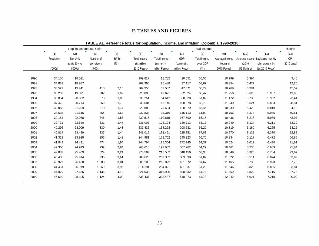
35
F. TABLES AND FIGURES
Inflation
(1) (2) (3) (4) (5) (6) (7) (8) (9) (10) (11) (12)
Population Tax Units Number of (3)/(2) Total income Total income GDP Total income Average income Average income Legislated monthly CPI
adults 20+ yo tax returns (%) (th. million (current th. (current th. over GDP (thousand (2010 Min. wage x 14 (2010 base)
('000s) ('000s) ('000s) 2010 Pesos) million Pesos) million Pesos) (%) 2010 Pesos) US Dollars) (th. 2010 Pesos)
1990 34.130 18.521 199.817 18.782 28.651 65,55 10.789 5.394 9,40
1991 34.831 18.987 207.990 25.488 37.117 68,67 10.954 5.477 12,25
1992 35.521 19.441 418 2,15 209.350 32.587 47.371 68,79 10.769 5.384 15,57
1993 36.207 19.891 382 1,92 223.890 42.671 62.324 68,47 11.256 5.628 5.987 19,06
1994 36.854 20.332 378 1,86 233.251 54.612 80.520 67,82 11.472 5.736 5.902 23,41
1995 37.472 20.774 369 1,78 233.684 66.145 100.678 65,70 11.249 5.624 5.883 28,31
1996 38.068 21.209 370 1,74 229.889 78.604 120.079 65,46 10.839 5.420 5.819 34,19
1997 38.636 21.646 364 1,68 232.838 94.316 145.113 64,99 10.756 5.378 5.945 40,51
1998 39.184 22.088 346 1,57 230.515 110.815 167.500 66,16 10.436 5.218 5.936 48,07
1999 39.731 22.540 331 1,47 231.003 123.124 180.713 68,13 10.249 5.124 6.211 53,30
2000 40.296 23.009 330 1,43 237.435 138.228 208.531 66,29 10.319 5.160 6.255 58,22
2001 40.814 23.469 337 1,44 241.019 151.491 225.851 67,08 10.270 5.135 6.370 62,85
2002 41.329 23.938 356 1,49 244.981 163.762 245.323 66,75 10.234 5.117 6.472 66,85
2003 41.849 24.421 474 1,94 244.794 175.304 272.345 64,37 10.024 5.012 6.490 71,61
2004 42.368 24.913 732 2,94 260.615 197.652 307.762 64,22 10.461 5.230 6.609 75,84
2005 42.889 25.409 824 3,24 270.589 215.582 340.156 63,38 10.649 5.325 6.704 79,67
2006 43.406 25.914 936 3,61 285.626 237.332 383.898 61,82 11.022 5.511 6.874 83,09
2007 43.927 26.438 1.008 3,81 303.108 265.822 431.072 61,67 11.465 5.733 6.923 87,70
2008 44.451 26.979 1.069 3,96 314.191 294.821 481.037 61,29 11.646 5.823 6.885 93,84
2009 44.979 27.536 1.136 4,13 321.038 313.906 508.532 61,73 11.659 5.829 7.115 97,78
2010 45.510 28.105 1.124 4,00 338.437 338.437 548.273 61,73 12.042 6.021 7.210 100,00
TABLE A1. Reference totals for population, income, and inflation. Colombia, 1990-2010
Population and Tax Units Total Income

36
Colombian $
expressed as
multiple of
average
income Colombian $
expressed as
multiple of
average
income Colombian $
expressed as
multiple of
average
income Colombian $
expressed as
multiple of
average
income Colombian $
expressed as
multiple of
average
income Colombian $
expressed as
multiple of
average
income Colombian $
expressed as
multiple of
average
income
1991 12.000.000 8,9 8.000.000 6,0 3.000.000 2,2 15.000.000 11,2
1992 20.300.000 12,1 13.500.000 8,1 5.100.000 3,0 39.000.000 23,3
1993 25.600.000 11,9 17.000.000 7,9 6.400.000 3,0 49.200.000 22,9
1994 31.200.000 11,6 20.800.000 7,7 7.800.000 2,9 60.100.000 22,4
1995 38.200.000 12,0 25.400.000 8,0 9.500.000 3,0 73.500.000 23,1
1996 46.100.000 12,4 30.700.000 8,3 11.500.000 3,1 88.800.000 24,0
1997 54.400.000 12,5 36.300.000 8,3 13.600.000 3,1 104.700.000 24,0
1998 63.100.000 12,6 42.100.000 8,4 15.800.000 3,1 121.500.000 24,2
1999 73.900.000 13,5 49.300.000 9,0 18.500.000 3,4 142.200.000 26,0
2000 80.800.000 13,4 53.900.000 9,0 20.200.000 3,4 155.500.000 25,9
2001 88.000.000 13,6 58.700.000 9,1 22.000.000 3,4 169.500.000 26,3
2002 95.100.000 13,9 63.400.000 9,3 23.800.000 3,5 183.200.000 26,8
2003 60.000.000 8,4 60.000.000 8,4 23.800.000 3,3 150.000.000 20,9
2004 60.000.000 7,6 60.000.000 7,6 25.000.000 3,2 80.000.000 10,1 80.000.000 10,1 50.000.000 6,3 50.000.000 6,3
2005 63.660.000 7,5 63.660.000 7,5 26.525.000 3,1 84.880.000 10,0 84.880.000 10,0 53.050.000 6,3 53.050.000 6,3
2006 66.888.000 7,3 66.888.000 7,3 27.870.000 3,0 89.183.000 9,7 89.183.000 9,7 55.740.000 6,1 55.740.000 6,1
2007 69.214.200 6,9 69.214.200 6,9 29.363.600 2,9 94.383.000 9,4 94.383.000 9,4 58.727.200 5,8 58.727.200 5,8
2008 72.778.200 6,7 72.778.200 6,7 30.875.600 2,8 99.243.000 9,1 99.243.000 9,1 61.751.200 5,7 61.751.200 5,7
2009 78.417.900 6,9 78.417.900 6,9 33.268.200 2,9 106.933.500 9,4 106.933.500 9,4 66.536.400 5,8 66.536.400 5,8
2010 100.012.515 8,3 81.031.500 6,7 34.377.000 2,9 110.497.500 9,2 110.497.500 9,2 68.754.000 5,7 68.754.000 5,7
Wealth criteria Expenditure criteria
Table A2. Tax filing thresholds. Personal income tax, Colombia 1991-2010
Gross Wealth
Total value of bank deposits
or financial investments Credit card expenditure Total expenditure
Employees Self-employee Other income receipients
Income criteria
Gross Income
Sources: Ley 49 de 1990; Decreto 2064 de 1992; Decreto 2511 de 1993; Decreto 2798 de 1994; Decreto 2321 de 1995; Decreto 2300 de 1996; Decreto 3049 de 1997; Decreto 3020 de 1998; Decreto 2587 de 1999; Decreto 2588 de
1999; Decreto 2661 de 2000; 2002: Ley 49 de 1990, Decreto 2794 de 2001; 2003: Ley 788 de 2002, Decreto 3257 de 2002; 2004: Ley 788 de 2002, Ley 863 de 2003; 2005: Ley 788 de 2002, Decreto 4344 de 2004, Decreto 44715 de
2005; Art 51 de Ley 1111 de 2006.
Notes: For filing purposes, individuals are categorised by source of income. An individual is considered an employee if she is not responsible for the sales tax and receives at least 80 percent of her gross income as wages. An
individual is considered a self-employee if she receives at least 80 per cent of her gross income as fees, commissions, and payment for services taxed at the source. If less than 80 per cent of an individual’s total gross income comes
from such sources (or if the individual does not have the receipts to prove so), then she is considered a “low-income taxpayer” (in the table referred to as 'Other income receipients').
The table reads as follow: in 2010, an individual was obliged to file for the income tax if (i) she was an employee with at least $100,012,515 in gross income; or (ii) she was a self-employee with at least $81,031,500 in gross income; or
(iii) she was a 'low-income' individual with at least $34,377,000 in gross income; or (iv) her gross wealth was at least $110,497,500; or (v) she had bank deposits and financial investments for at least $110,497,500; or (vi) her
expenditure through credit cards was at least $68,754,000; or (vii) her total expenditure was at least 68,754,000.

37
Professional risks CCF ICBF SENA
Bonus (Prima
de servicios)
Christmas
bonusHolidays
Unemployment
contributions
Interests on
unemployment
contributions
Unemployment
contribution for
unjustified
dismissal
Total employer employee employer employee employee employer employer employer employer Total employer employer employer employer employer employer
1992 7,0% 4,67% 2,33% 4,33% 2,17% 4,0% 3,0% 2,0% 9,0% 8,33% 8,33% 4,17% 8,33% 1,00% 4,17%
1993 7,0% 4,67% 2,33% 5,33% 2,67% 4,0% 3,0% 2,0% 9,0% 8,33% 8,33% 4,17% 8,33% 1,00% 4,17%
1994 8,0% 5,3% 2,7% 8,6% 2,9% 4,0% 3,0% 2,0% 9,0% 8,33% 8,33% 4,17% 8,30% 1,00% 4,17%
1995 12,0% 8,0% 4,0% 9,4% 3,1% 4,0% 3,0% 2,0% 9,0% 8,33% 8,33% 4,17% 8,33% 1,00% 4,17%
1996 12,0% 8,0% 4,0% 10,1% 3,4% 4,0% 3,0% 2,0% 9,0% 8,33% 8,33% 4,17% 8,33% 1,00% 4,17%
1997 12,0% 8,0% 4,0% 10,1% 3,4% 4,0% 3,0% 2,0% 9,0% 8,33% 8,33% 4,17% 8,33% 1,00% 4,17%
1998 12,0% 8,0% 4,0% 10,1% 3,4% 4,0% 3,0% 2,0% 9,0% 8,33% 8,33% 4,17% 8,33% 1,00% 4,17%
1999 12,0% 8,0% 4,0% 10,1% 3,4% 4,0% 3,0% 2,0% 9,0% 8,33% 8,33% 4,17% 8,33% 1,00% 4,17%
2000 12,0% 8,0% 4,0% 10,1% 3,4% 4,0% 3,0% 2,0% 9,0% 8,33% 8,33% 4,17% 8,33% 1,00% 4,17%
2001 12,0% 8,0% 4,0% 10,1% 3,4% 4,0% 3,0% 2,0% 9,0% 8,33% 8,33% 4,17% 8,33% 1,00% 4,17%
2002 12,0% 8,0% 4,0% 10,1% 3,4% 4,0% 3,0% 2,0% 9,0% 8,33% 8,33% 4,17% 8,33% 1,00% 4,17%
2003 12,0% 8,0% 4,0% 10,1% 3,4% 4,0% 3,0% 2,0% 9,0% 8,33% 8,33% 4,17% 8,33% 1,00% 4,17%
2004 12,0% 8,0% 4,0% 10,9% 3,6% 4,0% 3,0% 2,0% 9,0% 8,33% 8,33% 4,17% 8,33% 1,00% 4,17%
2005 12,0% 8,0% 4,0% 11,3% 3,8% 4,0% 3,0% 2,0% 9,0% 8,33% 8,33% 4,17% 8,33% 1,00% 4,17%
2006 12,0% 8,0% 4,0% 11,6% 3,9% 4,0% 3,0% 2,0% 9,0% 8,33% 8,33% 4,17% 8,33% 1,00% 4,17%
2007 12,5% 8,5% 4,0% 12,0% 4,0% 4,0% 3,0% 2,0% 9,0% 8,33% 8,33% 4,17% 8,33% 1,00% 4,17%
2008 12,5% 8,5% 4,0% 12,0% 4,0% 4,0% 3,0% 2,0% 9,0% 8,33% 8,33% 4,17% 8,33% 1,00% 4,17%
2009 12,5% 8,5% 4,0% 12,0% 4,0% 4,0% 3,0% 2,0% 9,0% 8,33% 8,33% 4,17% 8,33% 1,00% 4,17%
2010 12,5% 8,5% 4,0% 12,0% 4,0% 4,0% 3,0% 2,0% 9,0% 8,33% 8,33% 4,17% 8,33% 1,00% 4,17%
2011 12,5% 8,5% 4,0% 12,0% 4,0% 4,0% 3,0% 2,0% 9,0% 8,33% 8,33% 4,17% 8,33% 1,00% 4,17%
2012 12,5% 8,5% 4,0% 12,0% 4,0% 4,0% 3,0% 2,0% 9,0% 8,33% 8,33% 4,17% 8,33% 1,00% 4,17%
Earnings Solidaridad Subsistencia Total Risk class Min. contribution
Max.
contribution
expressed as
multiple of
minimum wage 1 0,348% 0,696%
2 0,435% 1,653%
0-4 0,00% 0,00% 0,00% 3 0,783% 4,089%
4-16 0,50% 0,50% 1,00% 4 1,740% 6,060%
5 3,219% 8,700%
0-4 0,00% 0,00% 0,00%
4-16 0,50% 0,50% 1,00%
16-17 0,50% 0,70% 1,20%
17-18 0,50% 0,90% 1,40%
18-19 0,50% 1,10% 1,60%
19-20 0,50% 1,30% 1,80%
>20 0,50% 1,50% 2,00%
Notes:
ICBF: Instituto Colombiano de Bienestar Familiar. CCF: Cajas de Compensación Familiar. SENA: Servicio Nacional de Aprendizaje.
The minimum wage is the SMLMV: Salario mínimo legal mensual vigente .
Sources: Mondragon-Velez et al. (2010), Santamaria et al. (2007), tax codes.
For employees, the contribution base is 100 per cent of the wage, or 70 per cent if the wage earner recieves an "integral" salary (i.e. one that includes bonuses, severance payments, etc.). Employer and employee can decide on an "integral" salary only
if the salary is greater than 10 times the minimum wage. There is a minimum cap equal to 1 minimum wage (SMLMV) and a maximum cap equal to 20 minimum wages (1993-2003) or 25 minimum wages (2003-2010). For self-employees, the social
security base is 40% of gross revenues, with the same minimum and maximum caps. Other non-wage labour costs not included in the table are work uniform and transport subsidies mandated by law for low-income employees.
up to 2002
since 2003
Professional risks
employer
Table A3. Social security contributions. Colombia, 1992-2012
Healthcare
employee
Parafiscales
Variable with
activity, and
ranging from
0.348% to 8.7%.
See below sub-
table Professional
risks .
Other charges on:
Pension
Employees
pay an
additional
contribution
variable with
earnings.
See below
sub-table
Fondo de
Solidaridad
Pensional .
Fondo de Solidaridad Pensional

38
Top 1% Top 0.5% Top 0.1% Top 0.05% Top 0.01% Top 0.001% Top 1-0.5% Top 0.5-0.1% Top 0.1-0.05% Top 0.05-0.01% Top 0.01-0.001%
(1) (2) (3) (4) (5) (6) (7) (8) (9) (10) (11)
1993 20,5 16,4 8,4 5,8 2,1 0,5 4,1 8,1 2,6 3,7 1,6
1994 20,5 16,3 8,1 5,4 1,9 0,4 4,2 8,2 2,7 3,5 1,5
1995 20,8 16,3 7,9 5,2 1,9 0,4 4,4 8,5 2,7 3,3 1,4
1996 21,3 16,6 7,7 5,0 1,8 0,5 4,7 8,9 2,6 3,2 1,4
1997 20,9 16,3 7,5 5,0 1,9 0,5 4,6 8,8 2,5 3,1 1,4
1998 19,8 15,4 7,0 4,6 1,8 0,5 4,4 8,4 2,3 2,9 1,3
1999 18,1 14,1 6,3 4,2 1,6 0,5 4,0 7,8 2,1 2,6 1,1
2000 17,3 13,7 6,1 4,1 1,6 0,5 3,6 7,6 2,0 2,5 1,1
2001 17,3 13,6 6,0 4,0 1,5 0,5 3,7 7,6 2,0 2,5 1,1
2002 18,0 13,9 6,0 4,0 1,6 0,5 4,0 7,9 1,9 2,5 1,0
2003 19,9 14,6 6,0 4,1 1,6 0,5 5,3 8,6 2,0 2,5 1,1
2004 17,8
2005 18,8
2006 19,9 15,0 7,6 5,7 2,9 1,1 4,9 7,4 1,9 2,8 1,7
2007 20,5 15,4 7,8 5,8 3,0 1,2 5,1 7,6 2,0 2,8 1,7
2008 20,3 15,2 7,5 5,5 2,7 1,0 5,1 7,7 2,0 2,8 1,7
2009 20,2 14,9 7,1 5,1 2,4 0,9 5,2 7,8 2,0 2,7 1,6
2010 20,4 15,2 7,4 5,4 2,6 1,0 5,2 7,8 2,0 2,7 1,6
Table A4. Top income shares, Colombia 1993-2010

39
Year Top 1% Top 0.5% Top 0.1% Top 0.05% Top 0.01% Top 0.001% Top 1-0.5% Top 0.5-0.1% Top 0.1-0.05%Top 0.05-0.01%Top 0.01-0.001% P99 P99.5 P99.9 P99.95 P99.99 P99.999
(1) (2) (3) (4) (5) (6) (7) (8) (9) (10) (11) (12) (13) (14) (15) (16) (17)
1993 230.512 369.780 940.536 1.295.779 2.357.322 5.155.611 91.244 227.091 585.292 1.030.394 2.046.401 59.778 121.001 437.261 719.338 1.339.673 3.055.851
1994 235.623 374.848 928.267 1.235.780 2.211.483 4.575.034 96.398 236.493 620.753 991.854 1.948.866 59.962 128.270 445.134 693.857 1.358.345 2.773.787
1995 233.552 367.828 883.127 1.160.345 2.083.984 4.619.739 99.276 239.003 605.908 929.435 1.802.233 61.386 129.582 463.626 676.167 1.282.169 2.533.038
1996 230.854 358.995 831.698 1.092.426 2.000.631 5.058.221 102.713 240.819 570.970 865.375 1.660.898 64.508 132.713 446.254 621.027 1.183.869 2.389.033
1997 224.281 349.992 807.712 1.067.061 2.002.839 5.452.980 98.571 235.562 548.363 833.117 1.619.490 61.169 129.759 421.155 585.690 1.109.382 2.335.843
1998 206.360 321.330 727.260 968.339 1.858.125 5.469.865 91.390 219.848 486.181 745.892 1.456.821 55.367 123.169 388.477 511.069 1.024.423 2.390.809
1999 185.494 289.048 648.230 865.205 1.685.004 5.078.892 81.940 199.252 431.255 660.256 1.307.905 48.503 112.517 343.573 455.144 909.675 2.112.837
2000 178.705 282.757 629.848 843.178 1.624.712 4.839.577 74.653 195.984 416.518 647.795 1.267.504 43.811 105.196 334.138 438.164 888.793 2.079.080
2001 177.806 280.068 614.734 826.155 1.591.328 4.906.464 75.544 196.401 403.314 634.861 1.222.979 43.995 107.115 325.542 424.060 857.645 2.014.915
2002 183.755 284.663 610.842 824.707 1.602.786 5.307.582 82.847 203.118 396.978 630.187 1.191.142 47.646 117.079 325.442 421.634 845.452 1.895.884
2003 199.671 293.001 604.810 817.271 1.580.073 5.220.327 106.341 215.049 392.350 626.570 1.175.601 73.588 124.501 324.005 438.093 826.713 1.901.168
2004 186.255 78.649
2005 200.197 83.709
2006 219.767 330.804 840.157 1.250.527 3.157.631 12.646.527 108.731 203.466 429.787 773.751 2.103.309 88.769 137.412 356.200 536.509 1.316.380 5.117.607
2007 234.973 353.770 891.919 1.323.053 3.382.314 13.864.922 116.176 219.232 460.784 808.238 2.217.580 94.203 147.808 383.783 570.290 1.346.454 5.526.192
2008 235.883 353.198 872.624 1.278.179 3.156.037 11.920.018 118.568 223.342 467.068 808.714 2.182.262 95.600 151.241 389.228 574.346 1.332.573 5.125.745
2009 235.106 347.936 830.763 1.197.711 2.841.088 10.213.877 122.275 227.229 463.816 786.867 2.021.889 98.664 155.293 390.589 567.750 1.279.498 4.681.815
2010 246.226 366.049 886.920 1.291.826 3.185.014 12.616.031 126.403 235.831 482.015 818.529 2.137.123 101.293 160.930 404.750 590.534 1.343.255 4.792.947
1993 115.256 184.890 470.268 647.890 1.178.661 2.577.805 45.622 113.545 292.646 515.197 1.023.200 29.889 60.500 218.631 359.669 669.836 1.527.926
1994 117.811 187.424 464.133 617.890 1.105.742 2.287.517 48.199 118.246 310.377 495.927 974.433 29.981 64.135 222.567 346.928 679.173 1.386.893
1995 116.776 183.914 441.563 580.172 1.041.992 2.309.869 49.638 119.502 302.954 464.718 901.116 30.693 64.791 231.813 338.083 641.085 1.266.519
1996 115.427 179.498 415.849 546.213 1.000.315 2.529.110 51.356 120.410 285.485 432.688 830.449 32.254 66.356 223.127 310.513 591.934 1.194.516
1997 112.141 174.996 403.856 533.531 1.001.419 2.726.490 49.285 117.781 274.182 416.558 809.745 30.585 64.879 210.578 292.845 554.691 1.167.921
1998 103.180 160.665 363.630 484.169 929.063 2.734.932 45.695 109.924 243.090 372.946 728.410 27.683 61.585 194.239 255.535 512.211 1.195.405
1999 92.747 144.524 324.115 432.603 842.502 2.539.446 40.970 99.626 215.628 330.128 653.953 24.251 56.258 171.786 227.572 454.838 1.056.419
2000 89.352 141.378 314.924 421.589 812.356 2.419.789 37.326 97.992 208.259 323.898 633.752 21.906 52.598 167.069 219.082 444.397 1.039.540
2001 88.903 140.034 307.367 413.077 795.664 2.453.232 37.772 98.200 201.657 317.431 611.490 21.997 53.557 162.771 212.030 428.823 1.007.458
2002 91.878 142.332 305.421 412.353 801.393 2.653.791 41.424 101.559 198.489 315.093 595.571 23.823 58.540 162.721 210.817 422.726 947.942
2003 99.836 146.501 302.405 408.635 790.037 2.610.163 53.171 107.524 196.175 313.285 587.800 36.794 62.250 162.002 219.046 413.357 950.584
2004 93.128 39.324
2005 100.099 41.854
2006 109.884 165.402 420.079 625.263 1.578.815 6.323.264 54.365 101.733 214.894 386.875 1.051.654 44.385 68.706 178.100 268.255 658.190 2.558.803
2007 117.486 176.885 445.959 661.527 1.691.157 6.932.461 58.088 109.616 230.392 404.119 1.108.790 47.102 73.904 191.891 285.145 673.227 2.763.096
2008 117.942 176.599 436.312 639.089 1.578.019 5.960.009 59.284 111.671 233.534 404.357 1.091.131 47.800 75.621 194.614 287.173 666.287 2.562.873
2009 117.553 173.968 415.382 598.855 1.420.544 5.106.938 61.138 113.615 231.908 393.433 1.010.944 49.332 77.647 195.295 283.875 639.749 2.340.908
2010 123.113 183.024 443.460 645.913 1.592.507 6.308.015 63.202 117.915 241.008 409.264 1.068.562 50.647 80.465 202.375 295.267 671.627 2.396.474
A. In 2010 Colombian Pesos (thousand)
Table A5. Incomes at the top. Colombia 1993-2010
B. In 2010 US Dollars

40
Wag
es
Sel
f-em
ploy
men
t
Ren
ts a
nd o
ther
capi
tal i
ncom
e
Inte
rest
and
othe
r fin
anci
al
inco
me
Bus
ines
s in
com
e
Irre
gula
r in
com
e
Wag
es
Sel
f-em
ploy
men
t
Ren
ts a
nd o
ther
capi
tal i
ncom
e
Inte
rest
and
othe
r fin
anci
al
inco
me
Bus
ines
s in
com
e
Irre
gula
r in
com
e
Wag
es
Sel
f-em
ploy
men
t
Ren
ts a
nd o
ther
capi
tal i
ncom
e
Inte
rest
and
othe
r fin
anci
al
inco
me
Bus
ines
s in
com
e
Irre
gula
r in
com
e
2006 29,7 17,3 42,2 2,7 5,0 3,1 23,6 17,4 47,9 2,8 4,9 3,4 12,2 14,7 60,7 3,0 4,8 4,5
2007 27,7 18,1 42,4 3,1 5,8 3,0 21,9 18,4 47,6 3,2 5,7 3,3 10,8 15,8 59,7 3,5 5,9 4,3
2008 28,3 18,1 42,3 3,5 5,6 2,1 22,5 18,5 47,7 3,6 5,5 2,2 11,3 16,0 60,6 4,0 5,6 2,6
2009 29,3 18,6 40,8 3,7 5,1 2,5 23,6 19,2 45,8 3,8 5,0 2,7 11,9 17,4 58,0 4,1 5,0 3,6
2010 28,6 18,4 41,2 3,5 5,5 2,9 23,0 18,8 45,9 3,6 5,5 3,2 11,5 16,5 57,6 4,1 6,0 4,3
Wag
es
Sel
f-em
ploy
men
t
Ren
ts a
nd o
ther
capi
tal i
ncom
e
Inte
rest
and
oth
er
finan
cial
inco
me
Bus
ines
s in
com
e
Irre
gula
r in
com
e
Wag
es
Sel
f-em
ploy
men
t
Ren
ts a
nd o
ther
capi
tal i
ncom
e
Inte
rest
and
oth
er
finan
cial
inco
me
Bus
ines
s in
com
e
Irre
gula
r in
com
e
Wag
es
Sel
f-em
ploy
men
t
Ren
ts a
nd o
ther
capi
tal i
ncom
e
Inte
rest
and
oth
er
finan
cial
inco
me
Bus
ines
s in
com
e
Irre
gula
r in
com
e
2006 9,3 12,7 65,0 3,1 4,9 5,2 5,1 7,1 73,1 3,2 4,8 6,8 3,5 0,4 80,0 3,6 4,2 8,3
2007 8,2 13,6 63,6 3,7 6,0 4,9 4,4 7,5 70,3 4,4 6,5 6,8 1,8 1,6 75,6 6,0 6,8 8,3
2008 8,6 13,9 64,9 4,2 5,5 2,8 4,8 8,7 72,7 4,8 5,6 3,3 3,5 1,6 81,9 6,7 3,0 3,3
2009 9,1 15,5 62,2 4,2 5,0 4,0 5,1 10,5 70,5 4,2 4,6 5,1 1,3 3,2 80,8 4,2 3,3 7,1
2010 8,5 14,5 61,2 4,5 6,3 5,0 4,3 8,7 68,3 5,7 6,7 6,4 1,2 2,6 74,2 7,5 7,6 7,0
Wag
es
Sel
f-em
ploy
men
t
Ren
ts a
nd o
ther
capi
tal i
ncom
e
Inte
rest
and
othe
r fin
anci
al
inco
me
Bus
ines
s in
com
e
Irre
gula
r in
com
e
Wag
es
Sel
f-em
ploy
men
t
Ren
ts a
nd o
ther
capi
tal i
ncom
e
Inte
rest
and
othe
r fin
anci
al
inco
me
Bus
ines
s in
com
e
Irre
gula
r in
com
e
Wag
es
Sel
f-em
ploy
men
t
Ren
ts a
nd o
ther
capi
tal i
ncom
e
Inte
rest
and
othe
r fin
anci
al
inco
me
Bus
ines
s in
com
e
Irre
gula
r in
com
e
Wag
es
Sel
f-em
ploy
men
t
Ren
ts a
nd o
ther
capi
tal i
ncom
e
Inte
rest
and
othe
r fin
anci
al
inco
me
Bus
ines
s in
com
e
Irre
gula
r in
com
e
Wag
es
Sel
f-em
ploy
men
t
Ren
ts a
nd o
ther
capi
tal i
ncom
e
Inte
rest
and
othe
r fin
anci
al
inco
me
Bus
ines
s in
com
e
Irre
gula
r in
com
e
2006 48,9 16,7 24,3 2,6 5,3 2,1 35,7 20,3 34,0 2,6 5,0 2,3 21,1 20,7 48,3 2,7 4,6 2,6 13,5 18,5 56,6 2,9 5,0 3,5 6,2 11,7 68,3 2,9 5,1 5,8
2007 46,0 17,1 26,0 2,9 6,0 2,1 33,5 21,2 34,7 2,8 5,5 2,2 18,4 22,1 48,5 2,9 5,4 2,7 12,2 20,0 56,5 2,9 5,5 2,9 6,3 11,8 66,6 3,3 6,4 5,7
2008 46,3 16,9 25,8 3,3 5,8 1,9 33,9 21,1 34,5 3,2 5,5 1,8 18,7 21,6 48,6 3,6 5,7 1,8 12,4 19,1 57,2 3,6 5,5 2,4 5,7 13,2 67,0 3,6 7,1 3,3
2009 46,0 16,9 26,0 3,6 5,4 2,1 34,6 20,8 34,1 3,6 4,9 1,9 19,5 22,5 47,1 3,7 4,9 2,3 12,7 20,1 54,6 4,2 5,4 3,1 7,3 14,7 64,4 4,2 5,4 4,0
2010 45,1 17,0 27,3 3,0 5,5 2,1 34,2 21,1 34,5 3,2 5,0 2,1 19,5 21,9 47,8 3,1 5,1 2,6 12,7 20,3 54,1 3,4 6,0 3,6 6,4 12,9 64,2 4,5 6,1 5,9
Table A6. Composition of income: income sources. Colombia 2006-2010
Notes: The table reads as follows. In 2006, the income of the top 1% group (100%) can be decomposed into wages (29.7%), self-employment income (17.3%), rents and other capital income (42.2%), interest and other financial income (2.7%), business income (5%)
and irregular income (3.1%).
Top 1% Top 0.5%
Top 0.05% Top 0.01% Top 0.001%
Top 0.1%
Top 1-0.5% Top 0.5-0.1% Top 0.1-0.05% Top 0.05-0.01% Top 0.01-0.001%
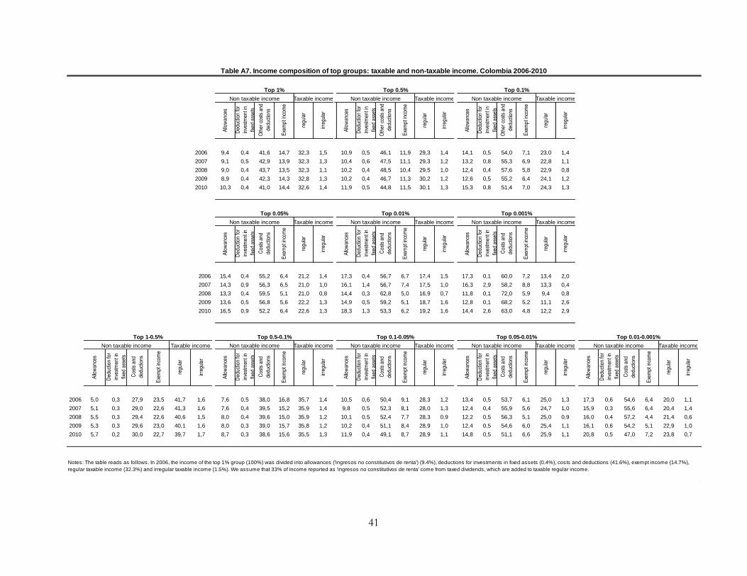
41
Allo
wan
ces
Ded
uctio
n fo
r
inve
stm
ent i
n
fixed
ass
ets
Oth
er c
osts
and
dedu
ctio
ns
Exe
mpt
inco
me
regu
lar
irreg
ular
Allo
wan
ces
Ded
uctio
n fo
r
inve
stm
ent i
n
fixed
ass
ets
Oth
er c
osts
and
dedu
ctio
ns
Exe
mpt
inco
me
regu
lar
irreg
ular
Allo
wan
ces
Ded
uctio
n fo
r
inve
stm
ent i
n
fixed
ass
ets
Oth
er c
osts
and
dedu
ctio
ns
Exe
mpt
inco
me
regu
lar
irreg
ular
2006 9,4 0,4 41,6 14,7 32,3 1,5 10,9 0,5 46,1 11,9 29,3 1,4 14,1 0,5 54,0 7,1 23,0 1,4
2007 9,1 0,5 42,9 13,9 32,3 1,3 10,4 0,6 47,5 11,1 29,3 1,2 13,2 0,8 55,3 6,9 22,8 1,1
2008 9,0 0,4 43,7 13,5 32,3 1,1 10,2 0,4 48,5 10,4 29,5 1,0 12,4 0,4 57,6 5,8 22,9 0,8
2009 8,9 0,4 42,3 14,3 32,8 1,3 10,2 0,4 46,7 11,3 30,2 1,2 12,6 0,5 55,2 6,4 24,1 1,2
2010 10,3 0,4 41,0 14,4 32,6 1,4 11,9 0,5 44,8 11,5 30,1 1,3 15,3 0,8 51,4 7,0 24,3 1,3
Allo
wan
ces
Ded
uctio
n fo
r
inve
stm
ent i
n
fixed
ass
ets
Cos
ts a
nd
dedu
ctio
ns
Exe
mpt
inco
me
regu
lar
irreg
ular
Allo
wan
ces
Ded
uctio
n fo
r
inve
stm
ent i
n
fixed
ass
ets
Cos
ts a
nd
dedu
ctio
ns
Exe
mpt
inco
me
regu
lar
irreg
ular
Allo
wan
ces
Ded
uctio
n fo
r
inve
stm
ent i
n
fixed
ass
ets
Cos
ts a
nd
dedu
ctio
ns
Exe
mpt
inco
me
regu
lar
irreg
ular
2006 15,4 0,4 55,2 6,4 21,2 1,4 17,3 0,4 56,7 6,7 17,4 1,5 17,3 0,1 60,0 7,2 13,4 2,0
2007 14,3 0,9 56,3 6,5 21,0 1,0 16,1 1,4 56,7 7,4 17,5 1,0 16,3 2,9 58,2 8,8 13,3 0,4
2008 13,3 0,4 59,5 5,1 21,0 0,8 14,4 0,3 62,8 5,0 16,9 0,7 11,8 0,1 72,0 5,9 9,4 0,8
2009 13,6 0,5 56,8 5,6 22,2 1,3 14,9 0,5 59,2 5,1 18,7 1,6 12,8 0,1 68,2 5,2 11,1 2,6
2010 16,5 0,9 52,2 6,4 22,6 1,3 18,3 1,3 53,3 6,2 19,2 1,6 14,4 2,6 63,0 4,8 12,2 2,9
Allo
wan
ces
Ded
uctio
n fo
r
inve
stm
ent i
n
fixed
ass
ets
Cos
ts a
nd
dedu
ctio
ns
Exe
mpt
inco
me
regu
lar
irreg
ular
Allo
wan
ces
Ded
uctio
n fo
r
inve
stm
ent i
n
fixed
ass
ets
Cos
ts a
nd
dedu
ctio
ns
Exe
mpt
inco
me
regu
lar
irreg
ular
Allo
wan
ces
Ded
uctio
n fo
r
inve
stm
ent i
n
fixed
ass
ets
Cos
ts a
nd
dedu
ctio
ns
Exe
mpt
inco
me
regu
lar
irreg
ular
Allo
wan
ces
Ded
uctio
n fo
r
inve
stm
ent i
n
fixed
ass
ets
Cos
ts a
nd
dedu
ctio
ns
Exe
mpt
inco
me
regu
lar
irreg
ular
Allo
wan
ces
Ded
uctio
n fo
r
inve
stm
ent i
n
fixed
ass
ets
Cos
ts a
nd
dedu
ctio
ns
Exe
mpt
inco
me
regu
lar
irreg
ular
2006 5,0 0,3 27,9 23,5 41,7 1,6 7,6 0,5 38,0 16,8 35,7 1,4 10,5 0,6 50,4 9,1 28,3 1,2 13,4 0,5 53,7 6,1 25,0 1,3 17,3 0,6 54,6 6,4 20,0 1,1
2007 5,1 0,3 29,0 22,6 41,3 1,6 7,6 0,4 39,5 15,2 35,9 1,4 9,8 0,5 52,3 8,1 28,0 1,3 12,4 0,4 55,9 5,6 24,7 1,0 15,9 0,3 55,6 6,4 20,4 1,4
2008 5,5 0,3 29,4 22,6 40,6 1,5 8,0 0,4 39,6 15,0 35,9 1,2 10,1 0,5 52,4 7,7 28,3 0,9 12,2 0,5 56,3 5,1 25,0 0,9 16,0 0,4 57,2 4,4 21,4 0,6
2009 5,3 0,3 29,6 23,0 40,1 1,6 8,0 0,3 39,0 15,7 35,8 1,2 10,2 0,4 51,1 8,4 28,9 1,0 12,4 0,5 54,6 6,0 25,4 1,1 16,1 0,6 54,2 5,1 22,9 1,0
2010 5,7 0,2 30,0 22,7 39,7 1,7 8,7 0,3 38,6 15,6 35,5 1,3 11,9 0,4 49,1 8,7 28,9 1,1 14,8 0,5 51,1 6,6 25,9 1,1 20,8 0,5 47,0 7,2 23,8 0,7
Table A7. Income composition of top groups: taxable and non-taxable income. Colombia 2006-2010
Top 1% Top 0.5% Top 0.1%
Non taxable income Taxable income Non taxable income Taxable income Non taxable income Taxable income
Top 0.05% Top 0.01% Top 0.001%
Non taxable income Taxable income Non taxable income Taxable income Non taxable income Taxable income
Top 1-0.5% Top 0.5-0.1% Top 0.1-0.05% Top 0.05-0.01% Top 0.01-0.001%
Taxable income Non taxable income Taxable income Non taxable income Taxable income
Notes: The table reads as follows. In 2006, the income of the top 1% group (100%) was divided into allowances ('ingresos no constitutivos de renta') (9.4%), deductions for investments in fixed assets (0.4%), costs and deductions (41.6%), exempt income (14.7%),
regular taxable income (32.3%) and irregular taxable income (1.5%). We assume that 33% of income reported as 'ingresos no constitutivos de renta' come from taxed dividends, which are added to taxable regular income.
Non taxable income Taxable income Non taxable income Taxable income Non taxable income
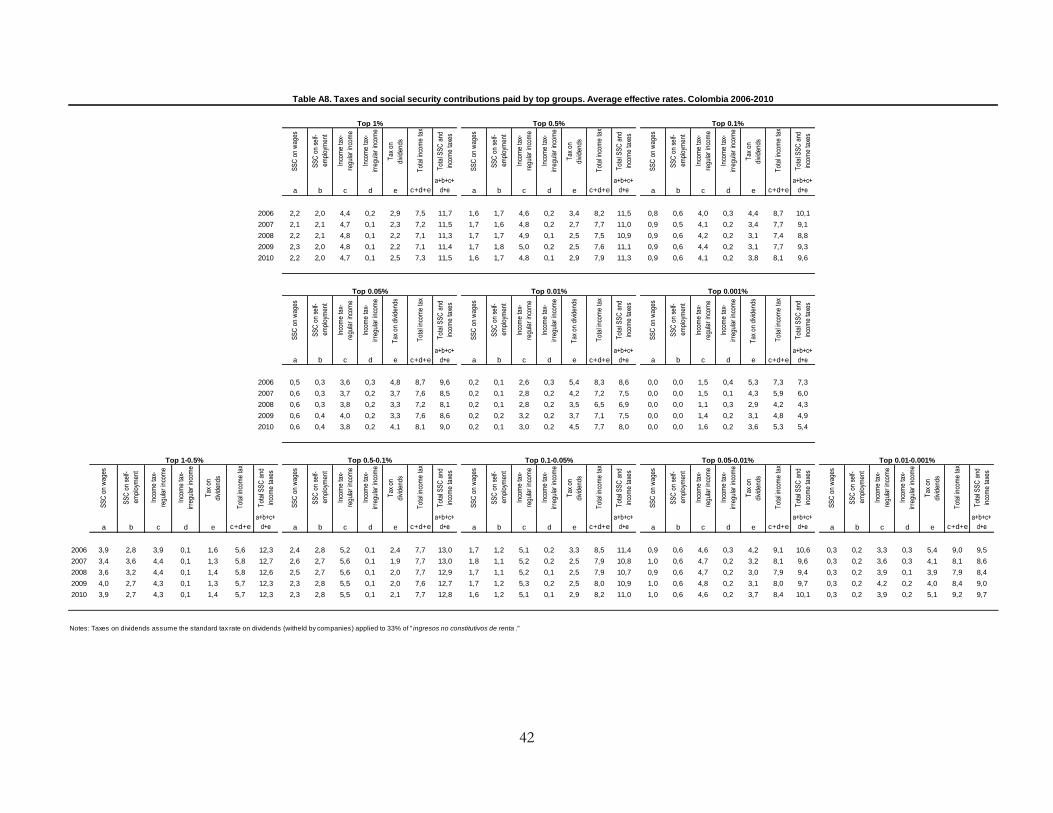
42
SS
C o
n w
ages
SS
C o
n se
lf-
empl
oym
ent
Inco
me
tax-
regu
lar
inco
me
Inco
me
tax-
irreg
ular
inco
me
Tax
on
divi
dend
s
Tot
al in
com
e ta
x
Tot
al S
SC
and
inco
me
taxe
s
SS
C o
n w
ages
SS
C o
n se
lf-
empl
oym
ent
Inco
me
tax-
regu
lar
inco
me
Inco
me
tax-
irreg
ular
inco
me
Tax
on
divi
dend
s
Tot
al in
com
e ta
x
Tot
al S
SC
and
inco
me
taxe
s
SS
C o
n w
ages
SS
C o
n se
lf-
empl
oym
ent
Inco
me
tax-
regu
lar
inco
me
Inco
me
tax-
irreg
ular
inco
me
Tax
on
divi
dend
s
Tot
al in
com
e ta
x
Tot
al S
SC
and
inco
me
taxe
s
a b c d e c+d+e
a+b+c+
d+e a b c d e c+d+e
a+b+c+
d+e a b c d e c+d+e
a+b+c+
d+e
2006 2,2 2,0 4,4 0,2 2,9 7,5 11,7 1,6 1,7 4,6 0,2 3,4 8,2 11,5 0,8 0,6 4,0 0,3 4,4 8,7 10,1
2007 2,1 2,1 4,7 0,1 2,3 7,2 11,5 1,7 1,6 4,8 0,2 2,7 7,7 11,0 0,9 0,5 4,1 0,2 3,4 7,7 9,1
2008 2,2 2,1 4,8 0,1 2,2 7,1 11,3 1,7 1,7 4,9 0,1 2,5 7,5 10,9 0,9 0,6 4,2 0,2 3,1 7,4 8,8
2009 2,3 2,0 4,8 0,1 2,2 7,1 11,4 1,7 1,8 5,0 0,2 2,5 7,6 11,1 0,9 0,6 4,4 0,2 3,1 7,7 9,3
2010 2,2 2,0 4,7 0,1 2,5 7,3 11,5 1,6 1,7 4,8 0,1 2,9 7,9 11,3 0,9 0,6 4,1 0,2 3,8 8,1 9,6
SS
C o
n w
ages
SS
C o
n se
lf-
empl
oym
ent
Inco
me
tax-
regu
lar
inco
me
Inco
me
tax-
irreg
ular
inco
me
Tax
on
divi
dend
s
Tot
al in
com
e ta
x
Tot
al S
SC
and
inco
me
taxe
s
SS
C o
n w
ages
SS
C o
n se
lf-
empl
oym
ent
Inco
me
tax-
regu
lar
inco
me
Inco
me
tax-
irreg
ular
inco
me
Tax
on
divi
dend
s
Tot
al in
com
e ta
x
Tot
al S
SC
and
inco
me
taxe
s
SS
C o
n w
ages
SS
C o
n se
lf-
empl
oym
ent
Inco
me
tax-
regu
lar
inco
me
Inco
me
tax-
irreg
ular
inco
me
Tax
on
divi
dend
s
Tot
al in
com
e ta
x
Tot
al S
SC
and
inco
me
taxe
s
a b c d e c+d+e
a+b+c+
d+e a b c d e c+d+e
a+b+c+
d+e a b c d e c+d+e
a+b+c+
d+e
2006 0,5 0,3 3,6 0,3 4,8 8,7 9,6 0,2 0,1 2,6 0,3 5,4 8,3 8,6 0,0 0,0 1,5 0,4 5,3 7,3 7,3
2007 0,6 0,3 3,7 0,2 3,7 7,6 8,5 0,2 0,1 2,8 0,2 4,2 7,2 7,5 0,0 0,0 1,5 0,1 4,3 5,9 6,0
2008 0,6 0,3 3,8 0,2 3,3 7,2 8,1 0,2 0,1 2,8 0,2 3,5 6,5 6,9 0,0 0,0 1,1 0,3 2,9 4,2 4,3
2009 0,6 0,4 4,0 0,2 3,3 7,6 8,6 0,2 0,2 3,2 0,2 3,7 7,1 7,5 0,0 0,0 1,4 0,2 3,1 4,8 4,9
2010 0,6 0,4 3,8 0,2 4,1 8,1 9,0 0,2 0,1 3,0 0,2 4,5 7,7 8,0 0,0 0,0 1,6 0,2 3,6 5,3 5,4
SS
C o
n w
ages
SS
C o
n se
lf-
empl
oym
ent
Inco
me
tax-
regu
lar
inco
me
Inco
me
tax-
irreg
ular
inco
me
Tax
on
divi
dend
s
Tot
al in
com
e ta
x
Tot
al S
SC
and
inco
me
taxe
s
SS
C o
n w
ages
SS
C o
n se
lf-
empl
oym
ent
Inco
me
tax-
regu
lar
inco
me
Inco
me
tax-
irreg
ular
inco
me
Tax
on
divi
dend
s
Tot
al in
com
e ta
x
Tot
al S
SC
and
inco
me
taxe
s
SS
C o
n w
ages
SS
C o
n se
lf-
empl
oym
ent
Inco
me
tax-
regu
lar
inco
me
Inco
me
tax-
irreg
ular
inco
me
Tax
on
divi
dend
s
Tot
al in
com
e ta
x
Tot
al S
SC
and
inco
me
taxe
s
SS
C o
n w
ages
SS
C o
n se
lf-
empl
oym
ent
Inco
me
tax-
regu
lar
inco
me
Inco
me
tax-
irreg
ular
inco
me
Tax
on
divi
dend
s
Tot
al in
com
e ta
x
Tot
al S
SC
and
inco
me
taxe
s
SS
C o
n w
ages
SS
C o
n se
lf-
empl
oym
ent
Inco
me
tax-
regu
lar
inco
me
Inco
me
tax-
irreg
ular
inco
me
Tax
on
divi
dend
s
Tot
al in
com
e ta
x
Tot
al S
SC
and
inco
me
taxe
s
a b c d e c+d+e
a+b+c+
d+e a b c d e c+d+e
a+b+c+
d+e a b c d e c+d+e
a+b+c+
d+e a b c d e c+d+e
a+b+c+
d+e a b c d e c+d+e
a+b+c+
d+e
2006 3,9 2,8 3,9 0,1 1,6 5,6 12,3 2,4 2,8 5,2 0,1 2,4 7,7 13,0 1,7 1,2 5,1 0,2 3,3 8,5 11,4 0,9 0,6 4,6 0,3 4,2 9,1 10,6 0,3 0,2 3,3 0,3 5,4 9,0 9,5
2007 3,4 3,6 4,4 0,1 1,3 5,8 12,7 2,6 2,7 5,6 0,1 1,9 7,7 13,0 1,8 1,1 5,2 0,2 2,5 7,9 10,8 1,0 0,6 4,7 0,2 3,2 8,1 9,6 0,3 0,2 3,6 0,3 4,1 8,1 8,6
2008 3,6 3,2 4,4 0,1 1,4 5,8 12,6 2,5 2,7 5,6 0,1 2,0 7,7 12,9 1,7 1,1 5,2 0,1 2,5 7,9 10,7 0,9 0,6 4,7 0,2 3,0 7,9 9,4 0,3 0,2 3,9 0,1 3,9 7,9 8,4
2009 4,0 2,7 4,3 0,1 1,3 5,7 12,3 2,3 2,8 5,5 0,1 2,0 7,6 12,7 1,7 1,2 5,3 0,2 2,5 8,0 10,9 1,0 0,6 4,8 0,2 3,1 8,0 9,7 0,3 0,2 4,2 0,2 4,0 8,4 9,0
2010 3,9 2,7 4,3 0,1 1,4 5,7 12,3 2,3 2,8 5,5 0,1 2,1 7,7 12,8 1,6 1,2 5,1 0,1 2,9 8,2 11,0 1,0 0,6 4,6 0,2 3,7 8,4 10,1 0,3 0,2 3,9 0,2 5,1 9,2 9,7
Notes: Taxes on dividends assume the standard tax rate on dividends (witheld by companies) applied to 33% of " ingresos no constitutivos de renta ."
Table A8. Taxes and social security contributions paid by top groups. Average effective rates. Colombia 2006-2010
Top 0.1%
Top 0.01% Top 0.001%
Top 1-0.5% Top 0.5-0.1% Top 0.1-0.05% Top 0.05-0.01% Top 0.01-0.001%
Top 1% Top 0.5%
Top 0.05%

43
0% 17% 25% 30%
1993 0 4.986.447 7.479.670 19.945.787
1994 0 6.087.454 9.131.181 24.349.817
1995 0 7.445.565 11.168.348 29.782.261
0% 20% 29% 35%
1996 0 8.992.754 13.489.131 35.971.015
1997 0 10.611.449 15.917.174 42.445.797
1998 0 12.309.281 18.463.922 49.237.125
1999 0 14.410.476 21.615.713 57.641.902
2000 0 15.759.296 23.638.944 63.037.184
2001 0 17.171.329 25.756.993 68.685.316
2002 0 18.558.772 27.838.159 74.235.089
0% 20% + 2% = 22% 29% + 2.9% = 31.9% 35% + 3.5% = 38.5%
2003 0 19.672.299 29.500.001 78.700.000
2004 0 20.400.001 32.400.001 78.000.001
2005 0 21.644.001 34.376.001 82.758.001
2006 0 22.742.001 36.119.001 86.954.001
0% 19% 28% 34%
2007 0 22.861.661 35.655.801 85.993.401
0% 19% 28% 33%
2008 0 24.038.861 37.491.801 90.421.401
2009 0 25.901.671 40.397.101 97.428.301
2010 0 26.764.951 41.743.501 100.675.501
Source: DIAN - SGAO - Estudios Económicos
Note: The table reads as follows. In 2010, taxable incomes in the range [0-26,764,951] face a marginal
tax rate of 0%; taxable incomes in the range [26,764,951-41,743,501] face a marginal tax rate of 19%;
and so on.
Table A9. Personal Income Tax Schedule: income brackets and rates
amounts in current Colombian Pesos

44
Top 1% Top 0.5% Top 0.1% Top 0.05% Top 0.01% Top 0.001% Top 1-0.5% Top 0.5-0.1% Top 0.1-0.05% Top 0.05-0.01% Top 0.01-0.001%
(%) (%) (%) (%) (%) (%) (%) (%) (%) (%) (%)
(1) (2) (3) (4) (5) (6) (7) (8) (9) (10) (11)
A 18,53 14,06 7,21 5,40 2,79 1,15 4,47 6,85 1,81 2,62 1,64
B 19,26 14,51 7,37 5,49 2,77 1,11 4,75 7,14 1,88 2,72 1,66
C 19,24 14,58 7,47 5,59 2,88 1,19 4,66 7,11 1,87 2,71 1,69
D 19,94 15,01 7,62 5,67 2,86 1,15 4,93 7,38 1,95 2,81 1,72
Notes: Sample A consists of filers not required to keep accountancy books in the 1993-2006 micro-data. Sample B
consists of filers not required to keep accountancy books in the weighted 2006-2010 micro-data. Sample C is equal to
sample A, plus individuals required to keep accountancy books from the weighted 2006-2010 micro-data. Sample D is
equal to sample B, plus individuals required to keep accountancy books from the weighted 2006-2010 micro-data.
Source: Author's calculations using tax data.
Sample
Table A10. Robustness check of top income shares in 2006
a-preferred b c d e f g
(%) (%) (%) (%) (%) (%) (%)
2006 19,9 21,6 19,9 17,3 19,4 16,7 12,5
2007 20,5 22,3 20,4 17,9 20,0 17,0 12,6
2008 20,3 22,0 20,2 17,7 19,9 16,8 12,4
2009 20,2 21,9 20,1 17,6 19,7 16,8 12,6
2010 20,4 22,1 20,4 17,5 19,9 17,2 13,0
Notes:
Column c. Income is equal to (a) minus the deduction for investments in fixed assets.
Column d. Income is equal to (a) minus 'ingresos no constitutivos de renta.'
Column e. Income is equal to (a) but excluding net taxable and non taxable irregular income.
Table A11. Top 1% income share under different definitions of income. Colombia 2006-2010
Column g. Income is equal to (a) but excludes 'other costs and deductions' (tax form 210) and 'other deductions' (tax form 110) completely.
Column a. For individuals not obliged to keep accountancy books: income = taxable income, plus exempt income, plus deductions for investments in fixed assets, plus 5/6 of
'other costs and deductions' (tax form definition), plus other non-taxable income, plus net taxable and non taxable irregular income.
For individuals obliged to keep accountancy books: income = taxable income, plus exempt income, plus deductions for investment in fixed income, plus 5/6 of 'other
deductions' (tax form definition), plus other non-taxable income, plus net taxable and non taxable irregular income.
Income definition (a) assumes that one-sixth of 'other costs and deductions' (individuals not obliged to keep accountancy books) and 'other deductions' (individuals obliged to
keep accountancy books) are costs incurred to obtain income.
Column b. Income is equal to (a) but includes 'other costs and deductions' (tax form 210) and 'other deductions' (tax form 110) completely.
Column f. Income is equal to (a) plus 1/2 of 'other costs and deductions' (individuals not obliged to keep accountancy books) and 'other deductions' (individuals obliged to keep
accountancy books). Thus, income defintion (f) includes in total 1/2 of these costs and deductions.

45
Top 1% Top 0.5% Top 0.1% Top 0.05% Top 0.01% Top 0.001% Top 1-0.5% Top 0.5-0.1% Top 0.1-0.05% Top 0.05-0.01%Top 0.01-0.001%
(%) (%) (%) (%) (%) (%) (%) (%) (%) (%) (%)
2006 28,1 30,0 32,7 33,2 32,8 34,7 24,5 28,5 31,7 32,8 33,8
2007 28,2 30,0 32,0 32,5 32,0 33,7 24,7 28,9 31,2 32,0 33,1
2008 27,9 29,6 31,3 31,7 31,4 32,6 24,7 28,7 30,7 31,4 32,3
2009 27,8 29,5 31,3 31,7 31,3 32,7 24,6 28,6 30,7 31,3 32,3
2010 27,9 29,5 31,3 31,7 31,3 32,8 24,6 28,6 30,6 31,3 32,3
Table A12. Weighted marginal tax rate of top groups, Colombia 2006-2010
Notes: The figures displays the histogram of taxable regular income. The data include the years 2007-2010. The statutory marginal
tax rate is displayed by the dashed line, and the kernel density of taxable regular income is plotted by the solid
line. The sample is restricted to filers not required to keep accountancy books. Taxable regular income has been converted
to CPI-adjusted "UVT" values. Bandwidth is 2 UVT in all estimations. In 2010, 2 UVT is equal to $49,100 pesos, or US$25.
Source: Author's calculations using tax data.
Panel A - Bunching at first kink Panel B - Bunching at top kink
FIGURE A1Bunching at first and top kink in Colombia

46
Source: Author's calculations using tax data.
FIGURE A2
Notes: The figure displays the histogram of taxable regular income. The data
include the years 2007-2010. The marginal tax rate schedule is displayed by the
dashed line, and the kernel density of taxable regular income is plotted by the
solid line. The sample is restricted to filers not required to keep accountancy
books. Taxable regular income has been converted to CPI-adjusted "UVT"
values. Bandwidth is 2 UVT in all estimations. In 2010, 2 UVT or $49,100 pesos,
around US$25.
Bunching: evidence by type of tax filer in Colombia

47
FIGURE A3
Notes: Wage earner is defined as an individual whose wages represent at least
99 per cent of total gross income. Taxable regular income has been converted to
UVT. Bandwidth is 2 UVT in all estimations. In 2010, 2 UVTis $49,100 pesos, or
approximately USD 25.
Source: Author's calculations using tax data and Stata code used by Chetty et al.
(2011).
Wage earners: bunching at first kink, ColombiaFIGURE A4
Notes: Taxable regular income has been converted to UVT. Bandwidth is 2 UVT
in all estimations. In 2010, 2 UVT or $49,100 pesos, or approximately US$25.
Source: Author's calculations using tax data and Stata code used by Chetty et al.
(2011).
Bunching at the top kink, all types of taxpayers, Colombia

48
REFERENCES Alvaredo, F. 2009. Top incomes and earnings in Portugal 1936-2005. Explorations in economic
history, 46, pp. 404-417.
Alvaredo, F. 2010. The Rich in Argentina over the Twentieth Century, 1932-2004, in A. B. Atkinson
and T. Piketty (eds.) Top Incomes: A Global Perspective, Oxford: Oxford University Press,
chapter 10, pp. 253-298.
Alvaredo, F. 2011. A note on the relationship between top income shares and the Gini cofficient.
Economic Letters, 110, 274-277.
Atkinson, A.B. 2007. Top incomes over the Twentieth century: A contrast between European and
English speaking countries. Oxford University Press. Chap. Measuring Top Incomes:
Methodological Issues.
Atkinson, A.B., and Piketty, T. 2007. Top incomes over the Twentieth century: A contrast between
European and English speaking countries. Oxford University Press.
Atkinson, A.B., and Piketty, T. 2010. Top incomes: A Global Perspective. Oxford University Press.
Avila, J., and Cruz, A. 2011. Analisis del impuesto sobre la renta para asalariados. DIAN
Subdirección de Gestión de Análisis Operacional, Cuaderno de Trabajo 042, June.
Bastani, S., and Selin, H. 2012. Bunching and non-bunching at kink points of the Swedish tax
schedule. Mimeo.
Burkhauser, R., Feng, S., Jenkins, S.P., and Larrimore, J. 2012. Recent trends in top income shares in
the United States: Reconciling estimates from March CPS and IRS tax return data. The Review
of Economics and Statistics, XCIV(2).
Burricand, C. 2012. Register use in income measurement: Transition from survey data to registers in
France, paper prepared as part of Net-SILC2 and presented in 2012 EU-SILC International
Conference Workshop, Vienna, 5 December 2012.

49
Chetty, R., Friedman, J.N., Olsen, T., and Pistaferri, L. 2011. Adjustment costs, firm responses, and
Micro vs. Macro labor supply elasticities: Evidence from Danish tax records. The Quarterly
Journal of Economics, 126, 749-804.
Deaton, A. 2005. Measuring poverty in a growing world (or measuring growth in a poor world).
Review of Economics and Statistics, 87(1), 1-19.
Ferreira, F.H.G., and Ravallion, M. (2008). Global Poverty and Inequality : A Review of the
Evidence. World Bank Policy Research Working Paper 4623.
Gaviria, A., and Mejía, D. 2011. Políticas Antidroga en Colombia: Exitos, Fracasos y Extravíos.
Bogota, Colombia: University of Los Andes.
Gordon, R.H., and Slemrod, J. 2000. Does Atlas Shrug? The Economic Consequences of Taxing the
Rich. Cambridge, MA.: Harvard University Press. Chap. Are “real" responses to taxes simply
income shifting between corporate and personal tax bases?
Kleven, H., and Schultz, E.A. 2011. Estimating taxable income responses using Danish tax reforms.
Mimeo.
Kleven, H. Jacobsen, and Waseem, M. 2012. Behavioral responses to notches: Evidence from
Pakistani tax records. Mimeo.
le Maire, D., and Schjerning, B. 2012. Tax bunching, income shifting and self-employment. EPRU
Working Paper Series.
Londoño, J.L. 1995. Distribucion del ingreso y desarrollo economico: Colombia en el Siglo XX.
Tercer Mundo Editores.
Londoño Vélez, J. 2012. Income and Wealth at the Top in Colombia: An Exploration of Tax Records
1993-2010, Paris School of Economics Master Thesis.
Lustig, N. and López Calva, L. F. 2010. Declining inequality in Latin America: A decade of progress?,
Brookings/UNDP.

50
Moller, L.C. 2012. Fiscal policy in Colombia: Tapping its potential for a more equitable society. IDB
Working Paper Series 67623.
OECD. 2013. OECD Economic Surveys Colombia, Paris: OECD Publishing.
Olivera, M., Pachon, M., and Perry, G. 2010. The political economy of fiscal reform: The case of
Colombia, 1986-2006. IDB Working Paper Series No. 181.
Piketty, T. 2001. Les hauts revenus en France au XXe siècle: Inégalités et redistributions 1901-1998. Grasset.
Piketty, T. 2003. “Income Inequality in France, 1901–1998.” Journal of Political Economy, 111(5), pp.
1004–42.
Piketty, T., and Saez, E. 2007. Top Incomes over the Twentieth Century: A Contrast Between
Continental Europe and English-Speaking Countries. Oxford University Press. Chap. Income
and Wage Inequality in the United States 1913-2002.
Saez, E. 2010. Do taxpayers bunch at kinked points? American Economic Journal: Economic Policy,
2(3), 180-212.
Saez, E., Slemrod, J., and Giertz, S.H. 2012. The elasticity of taxable income with respect to marginal
tax rates: A critical review. Journal of Economic Literature, 50(1), 3-50.
Sanchez, F., Fernandez, A., and Armenta, A. 2007. Economia Colombiana en el Siglo XX: Un
Analisis Cuantitativo. Fondo de Cultura Economica. Chap. Historia monetaria de Colombia en
el Siglo XX: Grandes tendencias y episodios relevantes, pp. 313-383.
Szekely, M., and Hilgert, M. 1999. What's behind the inequality we measure: An investigation using
Latin American data. Inter-American Development Bank Working Paper No. 409.

51
CEQ WORKING PAPER SERIES
http://www.commitmentoequity.org
“Commitment to Equity Assessment (CEQ): Estimating the Incidence of Social Spending, Subsidies
and Taxes. Handbook,” by Nora Lustig and Sean Higgins, CEQ Working Paper No. 1, July
2011; revised January 2013.
“Commitment to Equity: Diagnostic Questionnaire,” by Nora Lustig, CEQ Working Paper No. 2,
2010; revised August 2012.
“The Impact of Taxes and Social Spending on Inequality and Poverty in Argentina, Bolivia,Brazil,
Mexico and Peru: A Synthesis of Results,” by Nora Lustig, George Gray Molina, Sean
Higgins, Miguel Jaramillo, Wilson Jiménez, Veronica Paz, Claudiney Pereira, Carola Pessino,
John Scott, and Ernesto Yañez, CEQ Working Paper No. 3, August 2012.
“Fiscal Incidence, Fiscal Mobility and the Poor: A New Approach,” by Nora Lustig and Sean
Higgins, CEQ Working Paper No. 4, September 2012.
“Social Spending and Income in Argentina in the 2000s: the Rising Role of Noncontributory
Pensions,” by Nora Lustig and Carola Pessino, CEQ Working Paper No. 5, January 2013.
“Explaining Low Redistributive Impact in Bolivia,” by Verónica Paz Arauco, George Gray Molina,
Wilson Jiménez Pozo, and Ernesto Yáñez Aguilar, CEQ Working Paper No. 6, January 2013.
“The Effects of Brazil’s High Taxation and Social Spending on the Distribution of Household
Income,” by Sean Higgins and Claudiney Pereira, CEQ Working Paper No.7, January 2013.
“Redistributive Impact and Efficiency of Mexico’s Fiscal System,” by John Scott, CEQ Working Paper
No. 8, January 2013.
“The Incidence of Social Spending and Taxes in Peru,” by Miguel Jaramillo Baanante, CEQ Working
Paper No. 9, January 2013.
“Social Spending, Taxes, and Income Redistribution in Uruguay,” by Marisa Bucheli, Nora Lustig,
Máximo Rossi and Florencia Amábile, CEQ Working Paper No. 10, January 2013.
“Social Spending, Taxes and Income Redistribution in Paraguay,” Sean Higgins, Nora Lustig, Julio
Ramirez (CADEP), Billy Swanson, CEQ Working Paper No. 11, February 2013.
“High Incomes and Personal Taxation in a Developing Economy: Colombia 1993-2010,” by
Facundo Alvaredo and Juliana Londoño Vélez, CEQ Working Paper No. 12, March 2013.

52
The CEQ logo is a stylized graphical representation of a Lorenz curve for a fairly unequal distribution of income (the bottom part of the C, below the diagonal) and a concentration curve for a very progressive transfer (the top part of the C).
What is CEQ?
Led by Nora Lustig (Tulane University) and Peter Hakim (Inter-American Dialogue), the Commitment to Equity (CEQ) project is designed to analyze the impact of taxes and social spending on inequality and poverty, and to provide a roadmap for governments, multilateral institutions, and nongovernmental organizations in their efforts to build more equitable societies. CEQ/Latin America is a joint project of the Inter-American Dialogue (IAD) and Tulane University’s Center for Inter-American Policy and Research (CIPR) and Department of Economics. The project has received financial support from the Canadian International Development Agency (CIDA), the Development Bank of Latin America (CAF), the General Electric Foundation, the Inter-American Development Bank (IADB), the International Fund for Agricultural Development (IFAD), the Norwegian Ministry of Foreign Affairs, the United Nations Development Programme’s Regional Bureau for Latin America and the Caribbean (UNDP/RBLAC), and the World Bank. http://commitmenttoequity.org