Embed Size (px)
Citation preview

High-Frequency Trading StrategyBased on Deep Neural Networks
Andres Ricardo Arevalo Murillo
Universidad Nacional de Colombia
Faculty of Engineering, Department of Systems and Industrial Engineering
Bogota D.C., Colombia
2018


High-Frequency Trading StrategyBased on Deep Neural Networks
Andres Ricardo Arevalo Murillo
This thesis is presented as a partial requirement to obtain the degree of
Doctor in Systems and Computer Engineering
Advisor:
German Jairo Hernandez Perez, Ph.D.
Research lines:
Applied Computing, Intelligent Systems and Natural Computing
Universidad Nacional de Colombia
Faculty of Engineering, Department of Systems and Industrial Engineering
Bogota D.C., Colombia
2018


For my beloved mother, father and sisters.
Thanks for always being there for me.


Abstract
Recent conceptual and engineering breakthroughs in Machine Learning (ML), particularly
in Deep Neural Networks (DNN), have revolutionized the Computer Science field and have
been responsible for astonishing breakthroughs in computer vision, speech recognition, facial
recognition, transaction fraud detection, automatic translation, video object tracking, nat-
ural language processing, and robotics, virtually disrupting every aspect of our lives. The
financial industry has not been oblivious to this revolution; since the introduction of the first
ML techniques, there have been efforts to use them as financial modeling and decision tools
rendering in some cases limited and other in cases useful results, but overall, not astonishing
results as in other areas. Some of the most challenging problems for ML come form finance,
for instance, price prediction whose solution will require not only the most advanced ML
techniques but also other non-standard and uncommon methods and techniques, giving the
origin of a new field called Financial ML, whose name has been coined by Lopez de Prado
last year.
Today, many hedge funds and investment banks have ML divisions, using all kinds of
data sources and techniques, to develop financial modeling and decision tools. Consequently,
ML is a part of the present and probably will be the future of the financial industry. In this
thesis, we use the Deep Neural Networks (DNN) and Recurrent Neural Networks (RNN),
two of the most advanced ML techniques, whose learning capabilities are enhanced using
the representational power of the Discrete Wavelet Transform (DWT), to model and predict
short-term stock prices showing that these techniques allow us to develop exploitable high-
frequency trading strategies.
Since high-frequency financial (HF) data are expensive, difficult to access, and immense
(Big Data), there is no standard dataset in Finance or Computational Finance. Therefore,
the chosen testing dataset consists of the tick-by-tick data of 18 well-known companies
from the Dow Jones Industrial Average Index (DJIA). This dataset has 348.98 millions of
transactions (17 GB) from January 2015 to July 2017.
After a long iterative process of data exploration and feature engineering, several features
were tested and combined. The tick-by-tick data are preprocessed and transformed using
the DWT with a Haar Filter. The final features consist of the sliding windows of two
variables: one-minute pseudo-log-returns (the logarithmic difference between one-minute
average prices) and the features generated by the DWT.

viii
These transformations, which are non-standard data transformations in finance, will
better represent the high-frequency behavior of Financial Time Series (FTS). Moreover,
the DNN predicts the next one-minute pseudo-log-return that can be transformed into the
next predicted one-minute average price. These prices will be used to build a high-frequency
trading strategy that buys (sells) when the next one-minute average price prediction is above
(below) the last one-minute closing price.
Results show that (i) the proposed DNN achieves a highly competitive prediction perfor-
mance in the price prediction domain given by a Directional Accuracy (DA) ranging from
64% to 72%. (ii) The proposed strategy yields positive profits, a max draw-down less or
equal to 3%, and an annualized volatility ranging from 3% to 9% for all stocks.
The main contribution is the innovative approach for predicting FTS. It includes the
combination of the advanced learning capabilities of the Deep Recurrent Neural Networks
(DRNNs), the representational power in frequency and time domains of the DWT, and the
idea of modeling time series through average prices.
Keywords: Short-term price Forecasting, High-frequency financial data, High-
frequency Trading, Algorithmic Trading, Deep Neural Networks, Discrete Wavelet
Transform, Computational Finance, Algorithmic trading.

Contents
Abstract vii
List of Figures xii
List of Tables xiii
Academic Products xv
1 Introduction 1
1.1 Algorithmic Trading . . . . . . . . . . . . . . . . . . . . . . . . . . . . . . . 1
1.2 Problem Statement and Motivation . . . . . . . . . . . . . . . . . . . . . . . 6
1.3 Hypothesis . . . . . . . . . . . . . . . . . . . . . . . . . . . . . . . . . . . . . 7
1.4 Thesis Structure . . . . . . . . . . . . . . . . . . . . . . . . . . . . . . . . . . 9
2 Financial Time Series 11
2.1 Time Series . . . . . . . . . . . . . . . . . . . . . . . . . . . . . . . . . . . . 11
2.2 Financial Time Series . . . . . . . . . . . . . . . . . . . . . . . . . . . . . . . 12
2.3 Price Prediction Arena . . . . . . . . . . . . . . . . . . . . . . . . . . . . . . 14
3 Wavelets 19
3.1 Haar Wavelet . . . . . . . . . . . . . . . . . . . . . . . . . . . . . . . . . . . 19
3.2 Discrete Wavelet Transform . . . . . . . . . . . . . . . . . . . . . . . . . . . 20
4 Deep Neural Networks 23
4.1 Artificial Neurons . . . . . . . . . . . . . . . . . . . . . . . . . . . . . . . . . 23
4.2 Artificial Neural Networks Evolution . . . . . . . . . . . . . . . . . . . . . . 24
4.3 Deep Learning . . . . . . . . . . . . . . . . . . . . . . . . . . . . . . . . . . . 26
4.4 Recurrent Neural Networks . . . . . . . . . . . . . . . . . . . . . . . . . . . . 28
4.5 Artificial Neural Networks in Finance . . . . . . . . . . . . . . . . . . . . . . 30
5 DNN Short-Term Price Predictor 33
5.1 Dataset Description . . . . . . . . . . . . . . . . . . . . . . . . . . . . . . . . 33
5.2 Dataset Exploration . . . . . . . . . . . . . . . . . . . . . . . . . . . . . . . 34

x CONTENTS
5.3 Pseudo-log Returns . . . . . . . . . . . . . . . . . . . . . . . . . . . . . . . . 37
5.4 Dataset Preprocessing . . . . . . . . . . . . . . . . . . . . . . . . . . . . . . 38
5.5 Modeling . . . . . . . . . . . . . . . . . . . . . . . . . . . . . . . . . . . . . . 38
6 High-Frequency Strategy 41
6.1 Baseline Strategy . . . . . . . . . . . . . . . . . . . . . . . . . . . . . . . . . 41
6.2 Proposed Strategy . . . . . . . . . . . . . . . . . . . . . . . . . . . . . . . . 43
6.3 Simulation of the Proposed Strategy . . . . . . . . . . . . . . . . . . . . . . 43
7 Experiments and Results 45
7.1 Experimental Setting: Short-Term Price Predictor . . . . . . . . . . . . . . . 45
7.2 Experiment and Results: Price Predictor . . . . . . . . . . . . . . . . . . . . 49
7.3 High-Frequency Trading Strategy Simulation . . . . . . . . . . . . . . . . . . 54
7.4 Trading Strategy Benchmark . . . . . . . . . . . . . . . . . . . . . . . . . . . 56
8 Conclusions and Recommendations 65
9 Opportunities for Future Research 69
Bibliography 71

List of Figures
1-1 Algorithmic Trading: Percentage of Market Volume. Source: [43]. . . . . . . 2
1-2 Reasons for Using Algorithmic Trading. Source: Modified from [105]. . . . . 3
1-3 Algorithmic Trading. Based on [5, 18, 23, 97]. . . . . . . . . . . . . . . . . . 4
1-4 Trend Indicator (Version I): The slope of a linear model. . . . . . . . . . . . 9
1-5 Trend Indicator (Version II): The parameters of linear model. . . . . . . . . 9
2-1 Financial Time Series Characteristics. . . . . . . . . . . . . . . . . . . . . . . 13
2-2 Quantitative Models for Price Prediction. Based on [25, 65, 77]. . . . . . . . 15
2-3 Simulation of Random Walks . . . . . . . . . . . . . . . . . . . . . . . . . . 17
3-1 Haar Wavelet. . . . . . . . . . . . . . . . . . . . . . . . . . . . . . . . . . . . 20
3-2 Cascading and Filter Banks. . . . . . . . . . . . . . . . . . . . . . . . . . . . 21
3-3 DWT Decomposition. . . . . . . . . . . . . . . . . . . . . . . . . . . . . . . . 22
4-1 Artificial Neuron. . . . . . . . . . . . . . . . . . . . . . . . . . . . . . . . . . 23
4-2 Artificial Neural Networks in Finance. . . . . . . . . . . . . . . . . . . . . . 24
4-3 Multilayer Perceptron. . . . . . . . . . . . . . . . . . . . . . . . . . . . . . . 25
4-4 Deep Learning Representation. Modified from [44]. . . . . . . . . . . . . . . 27
4-5 An Unrolled Recurrent Neural Network. . . . . . . . . . . . . . . . . . . . . 28
4-6 LSTM Architecture . . . . . . . . . . . . . . . . . . . . . . . . . . . . . . . . 30
4-7 GRU Architecture . . . . . . . . . . . . . . . . . . . . . . . . . . . . . . . . . 30
5-1 Stock: International Business Machines Corporation (IBM). . . . . . . . . . 33
5-2 Stock Steps: High Frequency Behavior. . . . . . . . . . . . . . . . . . . . . . 36
5-3 Correlations of the One-minute Closing Price Series . . . . . . . . . . . . . . 36
5-4 Example of 60 One-minute prices. . . . . . . . . . . . . . . . . . . . . . . . . 37
5-5 Data Preprocessing . . . . . . . . . . . . . . . . . . . . . . . . . . . . . . . . 38
5-6 Compressed Tick-by-Tick Series using DWT. . . . . . . . . . . . . . . . . . . 39
5-7 Deep Architecture. . . . . . . . . . . . . . . . . . . . . . . . . . . . . . . . . 40
6-1 Strategy Flowchart. . . . . . . . . . . . . . . . . . . . . . . . . . . . . . . . . 42
6-2 Modified Strategy Flowchart. . . . . . . . . . . . . . . . . . . . . . . . . . . 42

xii LIST OF FIGURES
6-3 Performance Comparison of the Strategies: The Walt Disney Company (DIS). 44
7-1 Performance of the Classic Statistical and Machine Learning Techniques. . . 50
7-2 Deep Neural Networks vs. ARIMA and Random Walk. . . . . . . . . . . . . 50
7-3 Performance of the Deep Neural Networks. . . . . . . . . . . . . . . . . . . . 51
7-4 Model Performance per Symbol during the Training and Testing Phases . . . 51
7-5 Average Number of Ticks per Minute vs. DA Performance . . . . . . . . . . 52
7-6 Average of the Standard Deviations per Minute of the Tick-by-Tick Log-
returns vs. DA Performance . . . . . . . . . . . . . . . . . . . . . . . . . . . 53
7-7 Hurst Exponents vs. Strategy Profits. . . . . . . . . . . . . . . . . . . . . . . 56
7-8 The Best-Performing Stock: Cisco Systems, Inc. (CSCO). . . . . . . . . . . 57
7-9 The Second Best-Performing Stock: Intel Corporation (INTC). . . . . . . . . 57
7-10 The Third Best-Performing Stock: Goldman Sachs Group, Inc. (GS). . . . . 58
7-11 The Third Worst-Performing Stock: American Express Company (AXP). . . 58
7-12 The Second Worst-Performing Stock: Chevron Corporation (CVX). . . . . . 59
7-13 The Worst-Performing Stock: DuPont Corporation (DD). . . . . . . . . . . . 59
7-14 Strategy Performance . . . . . . . . . . . . . . . . . . . . . . . . . . . . . . . 62
7-15 Cisco Inc. (CSCO): Estimated spread USD 0.01 . . . . . . . . . . . . . . . . 63
7-16 Apple Inc. (AAPL): Estimated spread USD 0.01 . . . . . . . . . . . . . . . . 63
7-17 Spread Analysis . . . . . . . . . . . . . . . . . . . . . . . . . . . . . . . . . . 64

List of Tables
4-1 Artificial Neural Networks Applications in Finance . . . . . . . . . . . . . . 31
5-1 Dataset Description. . . . . . . . . . . . . . . . . . . . . . . . . . . . . . . . 34
5-2 Minute Statistics of High-Frequency Data. . . . . . . . . . . . . . . . . . . . 35
7-1 Experimental Setting: Short-Term Price Predictor . . . . . . . . . . . . . . . 46
7-2 ARIMA Models. . . . . . . . . . . . . . . . . . . . . . . . . . . . . . . . . . 47
7-3 Paired Student’s t-tests: Significance Level α at 0.01. . . . . . . . . . . . . . 52
7-4 Training time. . . . . . . . . . . . . . . . . . . . . . . . . . . . . . . . . . . . 53
7-5 Experiment Setting: High-Frequency Trading Strategy . . . . . . . . . . . . 55
7-6 Simulation Results. . . . . . . . . . . . . . . . . . . . . . . . . . . . . . . . . 55
7-7 Experiment Setting: Trading Strategy Benchmark . . . . . . . . . . . . . . . 60
7-8 Strategy Benchmark. . . . . . . . . . . . . . . . . . . . . . . . . . . . . . . . 61

Academic Products
Awards
• Best Paper Award: Workshop on Engineering Applications 2017. September 27-29
2017. Cartagena, Colombia.
Publications
• Lecture Notes in Computer Science (ISSN 0302-9743 - Colciencias A2):
Arevalo A., Nino J., Hernandez G., Sandoval J. (2016) High-Frequency Trading Strat-
egy Based on Deep Neural Networks. In: Intelligent Computing Methodologies. ICIC
2016. Lecture Notes in Computer Science, vol 9773. Springer, Cham.
http://dx.doi.org/10.1007/978-3-319-42297-8_40
• Communications in Computer and Information Science (ISSN 1865-0929 -
Colciencias B): Arevalo A., Nino J., Hernandez G., Sandoval J., Leon D., Aragon
A. (2017) Algorithmic Trading Using Deep Neural Networks on High Frequency Data.
In: Figueroa-Garcıa J., Lopez-Santana E., Villa-Ramırez J., Ferro-Escobar R. (eds)
Applied Computer Sciences in Engineering. WEA 2017. Communications in Computer
and Information Science, vol 742. Springer, Cham.
https://doi.org/10.1007/978-3-319-66963-2_14
• Lecture Notes in Computer Science (ISSN 0302-9743 - Colciencias A2):
Arevalo A., Nino J., Leon D., Hernandez G., Sandoval J. (2018) Deep Learning and
Wavelets for High-Frequency Price Forecasting. In: Shi Y. et al. (eds) Computational
Science – ICCS 2018. ICCS 2018. Lecture Notes in Computer Science, vol 10861.
Springer, Cham. https://doi.org/10.1007/978-3-319-93701-4_29
• Lecture Notes in Computer Science (ISSN 0302-9743 - Colciencias A2):
Arevalo A., Leon D., Hernandez G. (2019) Portfolio Selection Based on Hierarchical
Clustering and Inverse-Variance Weighting. In: Rodrigues J. et al. (eds) Compu-
tational Science – ICCS 2019. ICCS 2019. Lecture Notes in Computer Science, vol
11538. Springer, Cham. https://doi.org/10.1007/978-3-030-22744-9_25

xvi ACADEMIC PRODUCTS
Conferences
• Arevalo A., Nino J., Hernandez G., Sandoval J., Leon D. (2016). A High-Frequency
Trading Strategy Using a Deep Multilayer Perceptron One-Minute Average Price Pre-
dictor. The 7th Annual Stevens Conference on High-Frequency Finance and Analytics.
Hoboken, NJ, USA.
• Arevalo A., Nino J., Hernandez G., Sandoval J. (2016) High-Frequency Trading Strat-
egy Based on Deep Neural Networks. In: Intelligent Computing Methodologies. Twelfth
International Conference on Intelligent Computing. ICIC 2016. Lanzhou, China.
• Arevalo A., Nino J., Hernandez G., Sandoval J., Leon D., Aragon A. (2017) Algo-
rithmic Trading Using Deep Neural Networks on High-Frequency Data. Workshop on
Engineering Applications. WEA 2017. Cartagena, Colombia.
• Arevalo A., Nino J., Leon D., Hernandez G., Sandoval J. (2018) Deep Learning and
Wavelets for High-Frequency Price Forecasting. International Conference on Compu-
tational Science. ICCS 2018. Wuxi, China.
• Arevalo A., Leon D., Hernandez G. (2019) Portfolio Selection Based on Hierarchical
Clustering and Inverse-Variance Weighting. International Conference on Computa-
tional Science. ICCS 2019. Faro, Portugal.
Posters
• Arevalo A., Hernandez G. (2017). High-Frequency Trading Strategy Based on Deep
Neural Networks. Cuarto Coloquio Doctoral de la Facultad de Ingenierıa. Universidad
Nacional de Colombia. Bogota, Colombia.
• Arevalo A., Hernandez G. (2017). Forecasting of One-minute Average Prices using
Deep Architectures. Quinto Coloquio Doctoral de la Facultad de Ingenierıa. Universi-
dad Nacional de Colombia. Bogota, Colombia.
• Arevalo A., Leon D., Hernandez G. (2019). Hierarchical Portfolio Construction using
Inverse-Variance Weighting. Septimo Coloquio Doctoral de la Facultad de Ingenierıa.
Universidad Nacional de Colombia. Bogota, Colombia.
Chapter 1
Introduction
Financial Markets are essential for the economy and society. They offer several advantages
that are crucial and central for economic development, which will eventually result in an
improvement in life quality [84, 45, 32, 98, 100]: Financial Markets can transform saving
into investment, improve the allocation of capital, affect the saving rate, provide liquidity
for critical actors to grow their businesses, increase efficiency for price discovery and reduce
costs by enabling a competitive environment among market participants, generate jobs and
give back more benefits to society.
However, our understanding of the markets is still very weak. Although we have a large
number of theory books with very elegant formulas supported by rigorous demonstrations,
which are quite difficult to follow by non-mathematicians, these usually have unrealistic sup-
positions and restrictions that do not model the actual behavior of the markets. When hedge
funds and investors try to create or improve new trading strategies, the expected behavior
of those strategies is to fail, because markets do not behave as theoretically expected. And
that is the same reason why only a few traders become successful and make big fortunes,
while most fail. The few who achieve success, have something in common: They are not
systematic and are governed by subjective and empirical criteria [28].
1.1 Algorithmic Trading
With the evolution of computers, financial markets also evolved. Since the last century,
human participants began to be replaced by machines. Now the traditional hedge funds
are moving to the quantitative world, a world that unlike the traditional one, is completely
systematic and is supported entirely by algorithmic trading strategies.
Algorithmic trading, defined as the use of automated programs that make trading orders,
has been widely used in the middle of the previous century [14]. Another more technical
definition of algorithmic trading is an online algorithm that opens and closes automatically
trading positions, seeking to make the best decision without knowing the future. This type of
2 CHAPTER 1. INTRODUCTION
íñ9îì9
îñ9ïì9
ðñ9
òì9
óñ9ôì9
ôï9 ôñ9
ì9
íì9
îì9
ïì9
ðì9
ñì9
òì9
óì9
ôì9
õì9
îììï îììð îììñ îììò îììó îììô îììõ îìíì îìíí îìíî
oP]Zu]d]vP
WvP(Dlsoµu
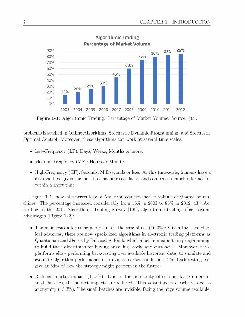
Figure 1-1: Algorithmic Trading: Percentage of Market Volume. Source: [43].
problems is studied in Online Algorithms, Stochastic Dynamic Programming, and Stochastic
Optimal Control. Moreover, these algorithms can work at several time scales:
• Low-Frequency (LF): Days, Weeks, Months or more.
• Medium-Frequency (MF): Hours or Minutes.
• High-Frequency (HF): Seconds, Milliseconds or less. At this time-scale, humans have a
disadvantage given the fact that machines are faster and can process much information
within a short time.
Figure 1-1 shows the percentage of American equities market volume originated by ma-
chines. The percentage increased considerably from 15% in 2003 to 85% in 2012 [43]. Ac-
cording to the 2015 Algorithmic Trading Survey [105], algorithmic trading offers several
advantages (Figure 1-2):
• The main reason for using algorithms is the ease of use (16.3%): Given the technolog-
ical advances, there are now specialized algorithms in electronic trading platforms as
Quantopian and JForex by Dukascopy Bank, which allow non-experts in programming,
to build their algorithms for buying or selling stocks and currencies. Moreover, these
platforms allow performing back-testing over available historical data, to simulate and
evaluate algorithm performance in previous market conditions. The back-testing can
give an idea of how the strategy might perform in the future.
• Reduced market impact (11.3%): Due to the possibility of sending large orders in
small batches, the market impacts are reduced. This advantage is closely related to
anonymity (13.3%). The small batches are invisible, facing the huge volume available.

1.1 Algorithmic Trading 3
Figure 1-2: Reasons for Using Algorithmic Trading. Source: Modified from [105].
• Price improvement (12.5%): The price discovery, described as the market process
whereby new information is impounded into asset prices, can be performed efficiently.
Furthermore, trades are executed at the best current price, because algorithms can
track the market conditions. So, they can decide at any time and immediately execute
it within milliseconds.
• Trader Productivity (10.4%): the risk of manual errors in placing the trades is reduced.
Besides, humans cannot make decisions on short timescales and consider all the avail-
able information, but machines can. This advantage is closely related to speed (4.3%):
With algorithmic trading, multiple market conditions can be automatically checked on
small-scale times.
• Commission rates (8.6%): Cost transactions can be reduced.
• Execution consistency (8.6%): Algorithms receive feedback from real-time data and
can continuously track the trading orders and market status.
4 CHAPTER 1. INTRODUCTION
Alg
orith
mic Tra
din
g
Arb
itrag
e
Op
po
rtun
ities
(HF
)
Ob
tain
free
-risk
pro
fit
Disco
ve
r p
rice
diffe
ren
tials
Sp
litting
up
larg
e o
rde
rs
(LF->
MF/H
F)
Op
era
te
larg
e o
rde
rs a
t be
st m
arke
t a
ve
rag
e
price
Min
imize
th
e m
arke
t im
pa
ct
Min
imize
e
xtra
costs
Mo
de
l Ba
sed
S
trate
gie
s
(LF, MF, H
F)
Fin
an
cial
Asse
ts P
riceM
od
ellin
g
Pre
dict
tren
d
pa
ttern
s
Cla
ssificatio
n
Po
rtfolio
C
on
figu
ratio
n
Ad
ve
rsaria
l P
red
ato
rs Alg
orith
ms
(LF, MF, H
F)
Disco
ve
r o
the
r a
lgo
rithm
s (A
dv
ersa
ries)
an
d b
ea
t th
em
.
Sn
iffing
a
lgo
rithm
s
Figu
re1-3
:A
lgorithm
icT
radin
g.B
asedon
[5,18,
23,97].

1.1 Algorithmic Trading 5
Financial markets have caught a lot of attention and interest from a large number of
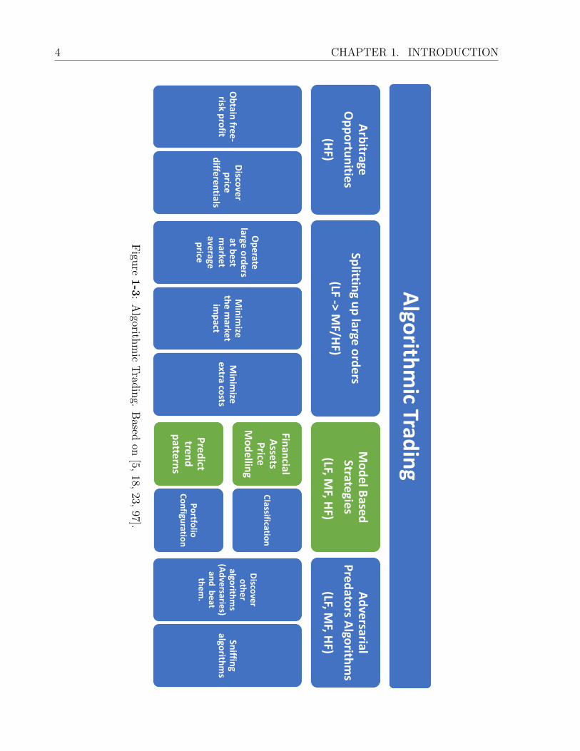
investors around the world. Figure 1-3 presents several types of algorithmic trading that
practitioners have widely used. There are four important families: Arbitrage opportunities,
algorithms for splitting up large orders, model-based strategies, and adversarial predators
algorithms.
Arbitrage opportunities, which operate at an HF scale, consist of discovering price differ-
entials between markets or exchanges rates. These strategies are risk-free profit and require
speed. For instance, if an asset is cheaper in the Market A than in the Market B, an investor
buys the asset in the Market A, and after the investor sells the asset rapidly in the Market B,
the investor will earn the price differential minus transaction costs. Given the fact that the
investor can calculate the final profit before making the transaction, this strategy is risk-free.
Given the conditions of the perfect market and a large number of market participants, the
arbitrage opportunities are increasingly challenging to find [3].
Additionally, not all strategies seek to gain profits. Other strategies also seek to avoid
impacts on the market. When someone needs to operate large orders, this agent must be
careful, if the agent sends the entire order, this action may cause price changes sharply, given
the laws of supply and demand. It may produce overruns and losses.
Therefore, there is another kind of algorithms that break-up large orders, so the large
order is hidden in small batches, and every batch can be operated at best market average
price, minimizing the market impact and extra costs. Those strategies are composed of two
components: the signal maker that operates at an LF scale, and the executor of the order
that performs the corresponding buy/sell orders at an MD or HF scale [48].
Also, there are algorithms specialized in detecting other algorithms and sniffing their
modus operandi, to take advantage and beat them. Those algorithms are called Beyond
Trading Algorithms or adversarial predators algorithms, which can operate at any time
scale (LF, MD, HF).
The model-based strategies, which operate at any time scale (LF, MD, HF), seek to
model some financial markets dynamics to identify behavior patterns and take advantage of
them, or even, to classify financial assets into different categories to build a robust portfolio
and hedge the risk. The modeling and predicting prices of financial assets have proved to
be arduous tasks that remain unsolved [25, 74]. This is mainly due to two reasons: First,
financial markets exhibit a nonlinear, complex, stochastic, non-stationary and heteroskedas-
tic behavior [65, 69, 87]. And second, markets also are a source of big data, then the task
of handling financial data becomes a tricky challenge that requires high technical knowledge
in computer science [28].
The most important approaches for price prediction are those based on simulation, an-
alytical models, and computational intelligence techniques. Since the 1800s, analytical ap-
proaches (classical statistical techniques and stochastic processes modeling) have dominated
the prediction arena [25, 65, 77]. Even though those classical models have been successful
for handling time series in many disciplines, they have very limited precision and accuracy

6 CHAPTER 1. INTRODUCTION
and low out-sample performance in the financial time series prediction [25].
Research during the last 20 years shows that computational intelligence approaches (more
specifically the techniques based on Machine Learning) are more effective in financial time
series tasks than analytical approaches [111, 59, 104, 85, 93, 16, 67, 116, 106, 34, 63, 21, 9,
64, 114, 81, 61, 19, 6, 55, 60, 109]. Computational Intelligence includes a wide variety of
techniques: Decision trees, Dynamic Bayesian Networks, Hidden Markov Models, Support
Vector Machines (SVMs), Kernel methods, Artificial Neural Networks (ANNs), and recently,
Deep Learning (DL), which has emerged as a useful technique for asset price modeling. DL
has proven to be able to learn complex representations of high-dimensional data and has
demonstrated significant results in [27, 36, 118, 33, 22, 31, 7, 99, 12, 39].
For the construction of portfolios, investment portfolio management theory (Markowitz’s
Portfolio Optimization, Stochastic portfolio theory, Risk parity, among others) and clustering
algorithms (Hierarchical clustering, k-means clustering, among others) are usually used.
Recent conceptual and engineering breakthroughs in Machine Learning (ML), particu-
larly in Deep Learning (DL) whose lead developers Bengio, Hinton and LeCun were awarded
last year with the most prestigious award in Computer Science, the ACM A.M. Turing Award
[2], have revolutionized the Computer Science field and have been responsible for astonishing
breakthroughs in computer vision, speech recognition, facial recognition, transaction fraud
detection, automatic translation, video object tracking, natural language processing, and
robotics, virtually disrupting every aspect of our lives. The financial industry has not been
oblivious to this revolution. However, there have not been astonishing results in the financial
industry as in other areas.
Now it is recognized that some of the most challenging problems for ML come from Fi-
nance, for instance, price prediction, whose solution will require not only the most advanced
ML techniques but also require to develop their methods and techniques, giving the origin
of a new field called Financial ML, whose name has been coined by Lopez de Prado last
year [28]. Consequently, ML is a part of the present and probably will be the future of the
financial industry. This transformation is also propelling developments in financial theory
by looking for answers of why and how the ML models can capture more effectively the
complex behavior of financial markets.
1.2 Problem Statement and Motivation
Financial markets play a vital role in our society since they affect economic growth, and in
turn, can improve the people’s quality life [84, 45, 32, 98, 100]. Consequently, it is critical
to research and to improve our understanding of Financial Market Behaviour. Nevertheless,
the main problems of research in financial markets are: First, there is too much secrecy in
the industry. Second, there is no standard public data, then experiments and works are
difficult to replicate or compare. And finally, the worst of all problems: the industry and
academia are on different paths.
1.3 Hypothesis 7
Furthermore, the funds are moving to the world of algorithmic trading, motivated by
the machine learning revolution that has taken place in each of the aspects of our daily life.
While it is true that it is a revolution which still does not stop. On many occasions machine
learning is overrated and expectations are quite inflated. As a result, many quantitative
hedge funds fail, not because the techniques do not work, but they are misused [28].
The main motivation of this thesis is to help build a bridge between the financial industry
and academic research, providing experience and new approaches to improve understanding
of the markets, and showing results that ML techniques allow us to develop exploitable HF
trading strategies. Moreover, this thesis seeks to be a public base work for academic and
industrial research in financial machine learning. This field is a new multidisciplinary world
that is being born and will revolutionize the financial industry [28].
1.3 Hypothesis
The task of FTS prediction can be very challenging and quite frustrating. Like many data
science projects, this work started because there was some data available. Our case was
Apple’s tick-by-tick price series during the financial crisis of 2008. This dataset was more
difficult because it was of the real market in conditions of very high volatility (to see more
information about this dataset, see [7, 8]).
Naively, we tried to solve the problem of predicting short-term time series with an end-
to-end approach, that is, placing data as input to a machine learning model and letting the
model do everything. Although we used all the available models available in Caret package
(R) and scikit-learn package (Python) from Generalized Linear Models, Kernels, Support
Vector Machines, Decision Trees to Neural Networks (Multilayer perceptron, Elman network
and Jordan network), the out-sample performance always ranged from 50% to 54% of DA.
Frustrated by the results, we tried to create very deep neural networks with H2O (an
open-source software for big data analysis) that received huge time windows of prices, and
although the training times took days, the out-sample results did not improve significantly.
After reviewing the academic literature, we found many works adding unrealistic proce-
dures like smoothing all the time series, removing data outliers, over-fitting, among others.
But in a few papers, we saw something interesting: first, to include preprocessed informa-
tion like Rolling averages, technical indicators. And second, to add dimension reduction
procedures like PCA, auto-encoders, among others. We tried this new approach and the
out-sample performance increased to %58.
The feature engineering approach significantly improved the results but it was not enough.
After a long iterative process of data exploration and feature engineering, several features
were tested and combined. The found features were 3n+2 values: the current time (hour and
minute), the last n one-minute pseudo-log-returns, the last n one-minute standard deviations
of prices and the last n one-minute trend indicators, where n is the window size.
The trend indicator is calculated as the slope a of a fitted linear model on tick-by-tick

8 CHAPTER 1. INTRODUCTION
prices within the same minute. Let P be the price, t be the time in milliseconds within the
particular minute, and a and b be the linear model parameters. This statistical measurement
is defined as follows:
P = at+ b (1-1)
A small slope, close to 0, means that during the next minute, the price is going to remain
stable. A positive value means that the price is going to rise. A negative value means that
the price is going to fall. Change is proportional to distance value compared to 0; if the
distance is too far from zero, the price will rise or fall sharply. Figure 1-4 shows an example
of the trend indicator.
We proposed a model based on a deep multi-layer network that includes those features.
And this model achieved a %65 of DA [7, 8]. These non-conventional inputs proved to be
definitive for improving model performance.
The inclusion of the time as an additional input, suggested that there are specific patterns
with dynamic temporal dependencies in financial time series. However, a multi-layer network
usually learns static patterns over time [49]; therefore, a more powerful model that supports
temporal dynamics in its architecture (like Recurrent Neural Networks) could perform better.
Furthermore, those works proved feature engineering is a critical tool for enhancing the model
learning capabilities.
The major advantage of the trend indicator is to allow modeling the stock behavior at
an HF scale. Since the trend indicator was a key feature, we tried to improve it. The first
attempt was to make the linear model out of a polynomial of greater degree. Figure 1-5
shows an example.
However, this improvement did not work because the parameters of greater degrees of
the trend indicator were very close to 0 in all cases. We had to add a pre-processing step of
orthogonalize the polynomial and then to apply the linear model fitting. This orthogonal-
ization was key for increasing the model performance.
Hence, the hypotheses of this work were to use Deep Recurrent Neural Networks (DRNN),
such as Long Short-Term Models (LSTM) [52] and Gated Recurrent Units (GRU) [24], and
to enhance their learning capabilities with the Discrete Wavelet Transform (DWT) as an
input feature generator. Wavelets are useful for feature discovery [90, 80]. Unlike Fourier
transforms, they provide a decomposition of a signal, or time series, with a resolution in the
frequency and time domains. Wavelets are a useful way to extract key features from signals
to reproduce them without having to save or keep the complete signal [108]. Moreover, the
Haar Wavelet, which is the most simple orthogonal one, will be used for this work. Besides,
they have been used successfully in handling FTS [90, 80].
This work is an exploratory study that will focus on model-based strategies for price
predicting, specifically on those based on Recurrent Neural Networks (RNNs), which are a
subtype of ANNs that includes Deep Learning (DL) paradigms and techniques. The proposed

1.4 Thesis Structure 9
Figure 1-4: Trend Indicator (Version I): The slope of a linear model.
Figure 1-5: Trend Indicator (Version II): The parameters of linear model.
strategy will use the tick-by-tick time series (HF data) of 18 companies from the Dow Jones
Industrial Average Index (DJIA). We expect that wavelets in conjunction with DL allow
improving the stock prices predictions on high-frequency data concerning previous results
achieved in [8, 7].
1.4 Thesis Structure
This document continues as follows:
• Chapter 2 (Financial Time Series) presents background theory on Financial Time Series
(FTS). This chapter collects a characterization of FTS and shows a brief overview of
financial time series predictors.

10 CHAPTER 1. INTRODUCTION
• Chapter 3 (Wavelets) presents a background in wavelets analysis for FTS, emphasizing
in the Haar wavelet and the Discrete Wavelet Transform (DWT). This chapter also
shows the advantages of using this kind of transformation in FTS.
• Chapter 4 (Deep Neural Networks) presents background theory on DNNs and describes
some common ANNs architectures, emphasizing Recurrent Neural Networks (RNNs).
It also shows a brief timeline of ANNs and some remarkable applications in Finance.
• Chapter 5 (DNN Short-Term Price Predictor) proposes an innovative predictor based
on DNN, DWT, and pseudo-log-returns. This chapter formalizes the concept of pseudo-
log-returns and exposes the reason for using this non-standard data transformation.
• Chapter 6 (High-Frequency Strategy) presents the proposed trading strategy, which
uses high-frequency data and the predictor described in Chapter 5.
• Chapter 7 (Experiments and Results) presents the experiments and obtained results
for assessing the proposed predictor and the high-frequency strategy. The predictor
is compared against three different alternatives of DNN architectures, ARIMA model,
a Random Walk (RW) simulation, and other seven techniques of similar complexity:
Linear regression, Ridge, Lasso, Bayesian ridge, Stochastic Gradient Descent (SGD)
Regressor, Decision trees and Support Vector Regression (SVR). Besides, this chapter
presents a comparison of the proposed strategy with three other types: Buy & Hold
Strategy, Relative Strength Index (RSI) strategy with six different time windows, and
one-minute random trading strategy.
• Chapter 8 (Conclusions) shows conclusions that range from the use of the DWT, the
inclusion of DL, advantages of the feature engineering, the power of the pseudo-log-
returns and the suitability of liquid stocks for high-frequency trading strategies, to the
discussion of the success of the proposed strategy.
• Finally, Chapter 9 (Possible Opportunities for Future Research) proposes recommen-
dations for future research and possible extensions. It is a good starting point to extend
and improve this work.
Chapter 2
Financial Time Series
The study of time series is a universal topic and interesting for all practitioners and re-
searchers who perform quantitative analyses on data indexed by time. Time series are used
in any domain of knowledge that involves temporal measurements of a phenomenon. There
are many properties and types of time series, but the most valuable ones are the stochastic se-
ries which are the realization of a stochastic process [107]. This chapter presents background
theory on Financial Time Series (FTS) and shows a brief overview of FTS predictors.
2.1 Time Series
A time series X is an ordered collection of temporal observations Xt indexed by an index
set T [40]. A time series is formally defined as follows:
X = X1, X2, . . . = Xt : t ∈ T (2-1)
The study of time series focuses on two areas [79]:
• Time series analysis: This area focuses on the study of methods and techniques for
analyzing and characterizing series behavior.
• Time series prediction: This area focuses on the study of models for predicting aptly
future observations of a time series X based on previously observed values. These
models produce an approximate time series Y which is expected to be as close as
possible to the actual time series X.
Given that this work focuses on time series prediction and proposes a prediction model,
it is required to define how to measure the quality of an estimator or model. According to
the reviewed literature, the most common measures in Finance are [57]:

12 CHAPTER 2. FINANCIAL TIME SERIES
• Mean Squared Error (MSE): It measures the average of the squares of the errors
(the difference between all predicted time series values Yt and expected time series
values Xi). Although it is widely used in Finance and many other disciplines, it has
a serious disadvantage for handling outliers and variables scales. Hence, it is a scale-
dependent measure.
MSE =1
n
n∑t=1
(Xt − Yt)2 (2-2)
• Directional Accuracy (DA): It measures the percentage of the predicted directions
(Up, Down, None) that match with the ones of the time series X. Since DA is unaf-
fected by outliers and variables scales, it is a scale-independent measure. As a result,
this measure is widely used in Finance [96].
DA =100%
n− 1
n∑t=2
1sign(Xt−Xt−1)=sign(Yt−Tt−1) (2-3)
where 1A is an indicator function, defined as follows:
1A = f(x) =
1, A = True
0, A = False(2-4)
and sign is a sign function, defined as follows:
sign(x) =
−1, x < 0
0, x = 0
1, x > 0)
(2-5)
2.2 Financial Time Series
A Financial Time Series (FTS) is a collection of financial data points such as asset price,
traded volume, earnings reports, business health data, or any transformation of the previous
ones.
In recent years, great interest has been generated in the FTS prediction field, since
a precise and accurate prediction of asset prices or stock market indexes is an indispens-
able tool for investment decision-making. However, FTS are characteristically stochastic
and non-stationary [47, 1, 103]. Stochastic refers to the property of being randomly deter-
mined, whereas, non-stationary refers to the characteristic of having means and variances
that change over time.

2.2 Financial Time Series 13
FTS
Stochastic
Non-stationary
Heteroskedas-
ticity
Nonlinearity
Big Data
(HF FTS)
Figure 2-1: Financial Time Series Characteristics.
As a result of the stochastic and non-stationary properties, an FTS has a probability
density function that changes over time. Moreover, an FTS is conditional heteroscedastic,
namely the variability of an FTS across time is dependent on other variables. Hence, FTS
prediction is considered one of the most challenging tasks of the time series prediction arena.
In many cases, the study of FTS has inspired the evolution of the forecasting methods, which
apply to time series in general [107, 47, 26].
Furthermore, FTS collect data of price changes over time due to the interaction of market
participants and their expectations, therefore, it is a hard challenge, because financial mar-
kets exhibit the seven properties inherent of complex systems [83]: “Historicity, Irreversible,
Thoroughgoing change, Propagation across multiple levels, Multiple modes of projection,
Emergence and Sensibility to externalities”. Moreover, financial markets are a source of
big data, then FTS becomes a tricky challenge to manipulate all this massive amount of
information. Figure 2-1 shows the summary of FTS characteristics.
These characteristics are shaped by the action of many market participants acting actively
in financial markets at different times, with a variety of investments size, making them
difficult to analyze. It is common to transform them into a difference series, such as log-
returns, in order to obtain a stationary time series and thus reduce somewhat its complexity
and difficulty.

14 CHAPTER 2. FINANCIAL TIME SERIES
Log-return is a continuously compounded return on an investment. Let pt and pt−1 be
the current and previous closing price, respectively.
Rt = lnptpt−1
· 100% = (ln pt − ln pt−1) · 100%
pt =pt−1 · eRt
100%
(2-6)
Figure 2-2 shows a summary of quantitative models for price prediction. There are
three important families of quantitative models for price prediction: Simulation approaches,
Analytical approaches, and Computational intelligence. Simulation approaches are Game
theory simulations and Monte Carlo simulations.
2.3 Price Prediction Arena
Analytical approaches consist mainly of statistical models and stochastic processes model-
ing. Statistical models were popular in the forecasting arena since the 1800s [77]. They
include many classic models such as Linear Regression (LR), Exponential Smoothing (ES),
Autoregressive (AR), Moving Averages (MA), Autoregressive Integrated Moving Average
(ARIMA) and Autoregressive Conditional Heteroskedasticity (GARCH).
Econometric models have dominated the time series prediction arena, specifically, linear
statistical methods such as Auto-Regressive Integrated Moving Average (ARIMA). This
model consists of the combination of the models AR and MA, and the statistical technique
of differentiation [15].
The AR model represents a random process in which the output variable depends linearly
on its previous values plus a white noise[78]. The white noise εt is a random signal which
has equal intensity at any frequencies [17]. The AR(p) model is defined as follows:
Xt = c+
p∑i=1
ϕiXt−i + εt (2-7)
where ϕi is the i-th parameter of the model, c is a constant and p the order of the
autoregressive model (number of time lags).
The MA model represents a random process in which the output variable depends linearly
on the current and previous values of a white noise signal [78]. The MA(q) model is defined
as follows:
Xt = µ+ εt +
q∑i=1
θiεt−i (2-8)

2.3 Price Prediction Arena 15
Qu
an
tita
tiv
eM
od
els
fo
r P
rice
pre
dic
tio
n
An
aly
tica
l A
pp
roa
che
s
Sta
tist
ica
l M
od
els
Mo
vin
g A
ve
rag
es
(MA
)
Lin
ea
r R
eg
ress
ion
(LR
)
Ex
po
ne
nti
al
Sm
oo
thin
g (
ES
)
AR
IMA
GA
RC
H
Sto
cha
stic
Pro
cess
es
Ra
nd
om
Wa
lks
(RW
)M
art
ing
ale
s
Ma
rko
v P
roce
sse
sG
au
ssia
n P
roce
sse
s
Ra
nd
om
Fie
lds
Lév
y P
roce
sse
s
Bro
wn
ian
Mo
tio
n
Po
isso
n P
roce
ss
Co
nti
nu
ou
s-T
ime
Ra
nd
om
Wa
lk(C
TR
W)
Sim
ula
tio
n A
pp
roa
che
s
Ga
me
Th
eo
ry
Sim
ula
tio
nM
on
teca
rlo
Co
mp
uta
tio
na
l In
tell
ige
nce
Ab
le t
o r
ep
rese
nt
a
pri
ori
kn
ow
led
ge
De
cisi
on
Tre
es
(DTs
)
Dy
na
mic
Ba
ye
sia
n
Ne
two
rks
(DB
Ns)
Hid
de
n M
ark
ov
Mo
de
ls (
HM
Ms)
No
t a
ble
to
re
pre
sen
t
a p
rio
ri k
no
wle
dg
e
Su
pp
ort
Ve
cto
r
Ma
chin
es
(SV
M)
Ke
rne
l M
eth
od
s
(KM
s)
Art
ific
ial
Ne
ura
l
Ne
two
rks
(AN
N)
Fig
ure
2-2
:Q
uan
tita
tive
Model
sfo
rP
rice
Pre
dic
tion
.B
ased
on[2
5,65
,77
].

16 CHAPTER 2. FINANCIAL TIME SERIES
where θi is the i-th parameter of the model, µ is the expectation of Xt and q the order
of moving average model (number of lagged errors in the prediction equation).
The ARMA model consists on the combination of the AR and MA models [112]. The
ARMA(p, q) model is defined as follows:
Xt = c+ εt +
p∑i=1
ϕiXt−i +
q∑i=1
θiεt−i (2-9)
The differentiation technique is a time series transformation that makes it stationary by
eliminating trend and seasonality [15]. The first-order differentiation is defined as follows:
X ′t = Xt −Xt−1 (2-10)
whereas, the second-order differentiation is defined as follows:
X ′′t = X ′t −X ′t−1 = (Xt −Xt−1)− (Xt−1 −Xt−2) = Xt − 2Xt−1 +Xt−2 (2-11)
An ARIMA model is a set of discrete time linear equations with noise, defined as follows:
ARIMA(p, d, q) =
(1−
p∑k=1
αkLk
)(1− L)dXt =
(1−
q∑k=1
βkLk
)εt. (2-12)
where L is the lag operator and d the degree of the differencing model (number of non-
seasonal differences needed to satisfy the stationary condition).
ARIMA models have been successful in the prediction of general time series. However,
they are not able to capture all financial markets complexities and non-linear relationships
[25]. Although ARIMA models usually perform well in in-sample datasets, they have a poor
performance in out-sample datasets.
Besides, stochastic processes consist of discrete-time and continuous-time models like
Random walks (RW), Martingales, Markov processes, Gaussian processes, Random fields,
and Levy processes, which are a generalization of Brownian motion, Poisson processes and
Continuous-Time Random Walk (CTRW).
Furthermore, the Brownian motion process, also known as the Wiener process in honor of
Norbert Wiener, is one of the best known Levy processes, has been widely used for modeling
price dynamics. Thus, it plays a vital role in quantitative finance [62].
In 1965, Eugene Fama published a prominent work about the consistency of the random
walk model and Efficient Market Hypothesis (EMH) [37]. EMH was considered a paradigm
theory in Finance by the middle of the 1970s arguing that asset prices capture and reflect
all the available information.
2.3 Price Prediction Arena 17
Figure 2-3: Simulation of 100 Random Walks with Parameters µ = 0.16, σ = 0.50 and
P0 = 40.
Several studies appeared in the 1930s [72, 38] and noticed that changes in stock prices
seem to follow a fair-game pattern, the second underpinning of the EMH. This hypothesis has
led to the random walk hypothesis, first exposed by Bachelier in 1900 [11], which states that
stock prices are random, hence, are unpredictable. A consequence is clear, is not possible to
“beat the market” and the prices follow a fair value.
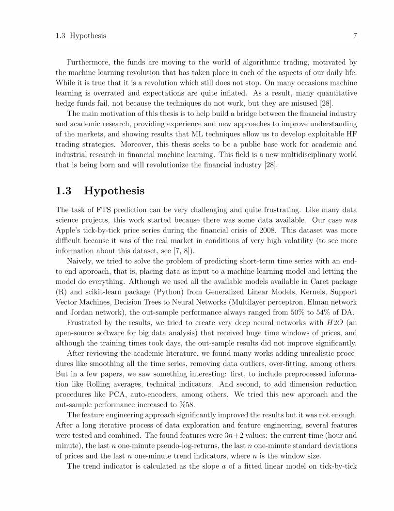
Figure 2-3 shows several simulations of a random walk based on a stochastic process
with drift and diffusion components, i.e. Brownian motion proposed as a benchmark model
to compare the proposed approach for FTS prediction.
The premise is that investors react instantaneously to any additional information re-
vealed, thus eliminating opportunities to obtain benefits persistently. Therefore, prices al-
ways fully reveal the information available and no profit can be obtained from information
based trading [70]. It leads to a random walk where the market is more efficient. The EMH
is the foundation of the theory that stock prices could follow a random walk. However, there
is no consensus on whether the market follows this paradigm or not. Our intuition is that the
market does not follow the EMH and is predictable to a certain degree that can be exploited
by a trading strategy.
As a result of the poor performance in out-sample datasets of classical techniques, other
techniques like machine learning methods have risen as an important alternative to handle
FTS, since those techniques can learn and predict the complex market patterns from data.
Research during the last 20 years shows that Computational intelligence approaches are more
effective in predicting FTS than Analytical approaches [59, 19, 109, 61].
Besides, Computational intelligence has two subfamilies: the models that can represent a
priori knowledge and those that cannot. For instance, Decision trees, Dynamic Bayesian Net-
works (DBNs), and Hidden Markov Models can represent a priori expert knowledge, whereas

18 CHAPTER 2. FINANCIAL TIME SERIES
Support Vector Machines (SVMs), Kernel methods, Artificial Neural Networks (ANNs) are
like black boxes which can learn complex representations, but it is not known precisely what
it does inside [26, 25, 65, 77]. ANNs were a favorite theme in data analysis during the 1980s.
In 1988, the first known application of ANN for price prediction was presented by [111].
They used ANNs for predicting IBM daily stock returns.
Recently, Deep Learning (DL) models have demonstrated greater effectiveness in several
tasks (classification and prediction), in different domains such as video analysis, audio recog-
nition, text analysis, and image processing. After the DL boom in 2009 [56], the number of
works related to finance has increased considerably.
Hence, DL has emerged as a useful technique for asset price modeling because it has
proven to be able to learn complex representations of high-dimensional data. This work will
focus on Deep Neural Networks (DNNs) like deep MLPs and RNNs, which are ones of the
most widely used techniques in DL.

Chapter 3
Wavelets
Given the fact that financial markets exhibit non-linear and cyclical behaviors [94], wavelets
are useful for feature discovery [90, 80]. Unlike Fourier transforms, they provide a decom-
position of a signal, or time series, with a resolution in the frequency and time domains.
Wavelets are a useful way to extract key features from signals in order to reproduce them
without having to save or keep the complete signal [108]. They have been used successfully
for handling FTS [90, 80].
A wavelet is a wave function with an average value of zero, which begins at zero, increases,
and then decreases back to zero. Therefore, wavelet has a finite duration [42]. Moreover,
wavelets are described by the mother wavelet function ψ(t) and the scaling function ϕ(t).
The function ψ(t) is a band-pass filter, whereas the function ϕ(t) is a filter that ensures that
all the spectrum is covered.
3.1 Haar Wavelet
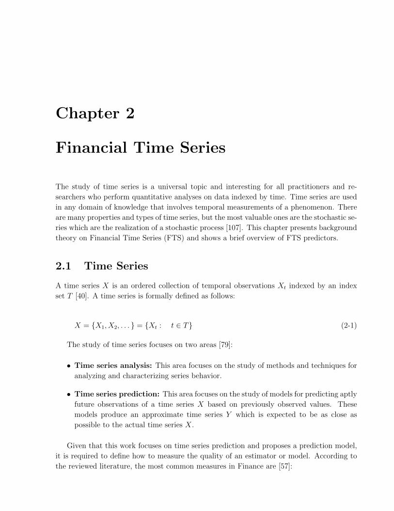
On 1909, Alfred Haar proposed the first and the simplest possible wavelet: the Haar wavelet
[46], as shown in Figure 3-1. Its mother wavelet function ψ(t) is defined as follows:
ψ(t) =
1 0 ≤ t < 1
2
−1 12≤ t < 1
0 otherwise
(3-1)
whereas its scaling function ϕ(t) is defined as follows:
ϕ(t) =
1 0 ≤ t < 1
0 otherwise(3-2)
The Haar wavelet has a technical disadvantage: It has discontinuities and hence it is
not a differentiable function. However, its discontinuities are an advantage for FTS analysis
20 CHAPTER 3. WAVELETS
−0.5 0.0 0.5 1.0 1.5
−1.5
−0.5
0.5
1.5
Haar Wavelet
t
Figure 3-1: Haar Wavelet.
because the discontinuities perfectly fit to handle signals with sudden transitions and jumps.
Moreover, the Haar wavelet is able to approximate uniformly any continuous real function
by linear combinations of ϕ(2kt+ l), where k ∈ N and l ∈ Z [108].
3.2 Discrete Wavelet Transform
The wavelet transform could be either continuous or discrete. Since financial time series are
discrete, the Discrete Wavelet Transform (DWT) is more suitable to handle FTS than the
Continuous Wavelet Transform (CWT) [108].
The DWT consist of the following steps [108, 86]: First, a signal x is passed simultane-
ously through a low-pass filter with impulse response g and a high-pass filter h. The filters
g and h are the dilated (by powers of two), reflected, and normalized versions of the mother
wavelet and scaling function, respectively. The filters are defined as follows:
h[n] =1√2jψ
(−t2j
)(3-3)
g[n] =1√2jϕ
(−t2j
)(3-4)
Second, given the fact that the filters g and h remove the half of the signal frequencies,
the half of the resulting samples can be discarded according to Nyquist’s rule, that is, the
resulting signal can be sub-sampled by 2. Finally, the high-pass filter produces the detail

3.2 Discrete Wavelet Transform 21
x[n] h[n] ↓ 2 W1
g[n] ↓ 2 V1 h[n] ↓ 2 W2
g[n] ↓ 2 V2 h[n] ↓ 2 W3
g[n] ↓ 2 V3
Figure 3-2: Cascading and Filter Banks.
or wavelet coefficients W , whereas the low-pass filter produces the approximation or scaling
coefficients V . The resulting signals, which are half the length of the original signal x, are
defined as follows:
W = yhigh = (x ∗ h) ↓ 2 =∞∑
k=−∞
x[k]h[2n− k] (3-5)
V = ylow = (x ∗ g) ↓ 2 =∞∑
k=−∞
x[k]g[2n− k] (3-6)
The previous transformation can be repeated multiple times in order to further increase
the frequency resolution. The first filter outputs will be named Level 1 coefficients, then
the transformation is applied again to the Level 1 scaling coefficients producing the Level 2
coefficients, and so on. The recursive transformation, which is presented in Figure 3-2, is
described as:
Vn =
(x ∗ g) ↓ 2 n = 1
(Vn−1 ∗ g) ↓ 2 otherwise(3-7)
Wn =
(x ∗ h) ↓ 2 n = 1
(Vn−1 ∗ h) ↓ 2 otherwise(3-8)
However, it has some disadvantages [50]. First, it requires that the length of the data
be 2j. Second, it is not shift-invariant. Finally, it may shift data peaks, causing wrong
approximations when compared to the original data.

22 CHAPTER 3. WAVELETS
0 500 1000 1500 2000
−4
04
x
X
t
T−0
W1
T−0
W2
T−0
W3
T−0
W4
T−0
W5
T−0
W6
T−0
V6
Figure 3-3: DWT Decomposition.
Figure 3-3 shows an example of the DWT decomposition over a sinusoidal signal with
noise. The signal is decomposed for six levels, and the figure shows the original signal, the
six levels wavelets coefficients W and the last level scaling coefficients V .
Moreover, wavelets possess additional advantages that help to overcome the FTS prop-
erties [50]: First, it does not require a strong assumption about the data generation process.
Second, it provides information in both time and frequency domains. Finally, it can locate
discontinuities in the data.
Chapter 4
Deep Neural Networks
Artificial Neural Networks (ANNs) are a hot topic in intelligent systems, machine learning,
data science, and other disciplines. This chapter presents the background theory on DNNs
and describes some common ANNs architectures, emphasizing Recurrent Neural Networks
(RNNs). It also shows a brief timeline of ANNs and some important applications in finance.
4.1 Artificial Neurons
ANNs are inspired by the biological neural networks on animals’ brains. Like their biological
analogous, they are a collection of connected units called neurons, where each neuron shares
information with other ones.
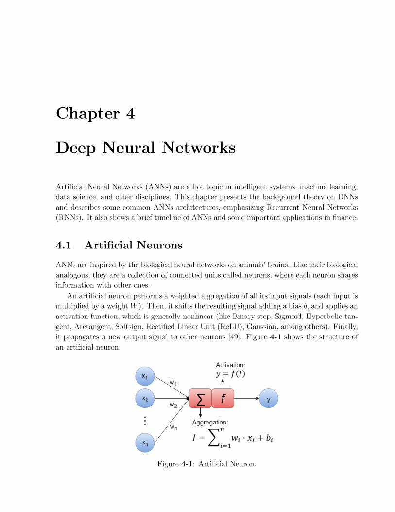
An artificial neuron performs a weighted aggregation of all its input signals (each input is
multiplied by a weight W ). Then, it shifts the resulting signal adding a bias b, and applies an
activation function, which is generally nonlinear (like Binary step, Sigmoid, Hyperbolic tan-
gent, Arctangent, Softsign, Rectified Linear Unit (ReLU), Gaussian, among others). Finally,
it propagates a new output signal to other neurons [49]. Figure 4-1 shows the structure of
an artificial neuron.
Figure 4-1: Artificial Neuron.

24 CHAPTER 4. DEEP NEURAL NETWORKS
ANNs have been widely used to predict FTS since the 1980s, due to its ability to identify
and learn intricate patterns from data in high dimensional spaces [41, 65, 87, 101].
4.2 Artificial Neural Networks Evolution
Figure 4-2 shows a brief timeline about neural networks and some of its applications in
Finance.
1943 · · · · · ·• Threshold Logic Unit (TLU) [75].
1950-1990 · · · · · ·• Evolution of ANN architectures (Multilayer, Recurrent,
Convolutional).
1974 · · · · · ·• Training of ANNs through Back-propagation algorithm [110].
1986 · · · · · ·•Efficient backpropagation [92].
The concept of Deep Learning was first introduced to the Machine
Learning community [30].
1988 · · · · · ·•First known MLP in finance: “Economic prediction using neural
networks: the case of IBM daily stock returns [111]”.
1989 · · · · · ·• MLP are universal approximators [54, 53].
Backpropagation for CNN [66].
1990 · · · · · ·•First known RNN in finance: “Stock price pattern recognition-a
recurrent neural network approach [59]”.
1997 · · · · · ·• Long Short-Term Memory (LSTM) [52].
2000 · · · · · ·• Deep Learning concept was introduced to ANN [4].
2006 · · · · · ·• Deep Learning foundations [51].
2009-Now · · · · · ·• Deep Learning “Big-Bang” [56].
2011-Now · · · · · ·• DL applications in Finance: [20, 33, 31].
2014 · · · · · ·• Gated Recurrent Unit (GRU) [24].
2015 · · · · · ·•First known LSTM in finance: “A LSTM-based method for stock
returns prediction: A case study of China stock market [22]”.
Figure 4-2: Artificial Neural Networks in Finance.

4.2 Artificial Neural Networks Evolution 25
Figure 4-3: Multilayer Perceptron.
In 1943, the Threshold Logic Unit (TLU) or Linear Threshold Unit was proposed in [75].
A TLU is the first neuron unit model. It performs a weighted sum of the boolean inputs
and returns a boolean value if the sum exceeds a predefined linear threshold.
From the 1950s to 1990s, multiple networks architectures were proposed, but all lacked
efficiency for learning algorithms. One of the first emerging ANN architectures was the Feed-
forward Neural Network (FNN). This kind of ANN consists of multiple connected artificial
neurons in such a way that there are no loops. In this way, the input signals always go
forward from input to output neurons.
There are many FNN sub-types, but the most common and famous architecture is the
Multilayer Perceptron (MLP). An MLP organizes its neurons in stacked layers of neurons.
Each layer is composed of neurons fully-connected to all the neurons in the next layer. There
are three kinds of layers: The input layer that contains all input neurons, the output layer
that contains all outputs neurons, and the hidden layers that contain all intermediate neurons
[49]. Figure 4-3 shows an MLP.
Convolutional Neural Networks (CNNs) are a variation of MLPs, whose layers are not
fully connected, but are locally connected [66]. As CNNs have fewer connections and pa-
rameters; it requires minimal processing to be fitted.
In 1974, Werbos was the first author who described the training of ANNs through the
back-propagation algorithm, which consists of the following steps [49, 91, 110]:

26 CHAPTER 4. DEEP NEURAL NETWORKS
1. To initialize the weights matrices and biases vectors with random values.
2. To compute the error between the network’s outputs and the desired outputs at the
output neurons.
3. To calculate the descent gradient based on the weights and biases that allows minimiz-
ing the error for all layers from output to input.
4. To update weights and biases according to gradients.
5. Repeat steps 2-4 until max iterations are reached, or another stopping criterion is
satisfied.
The idea behind this algorithm is that the error is propagated backward from the output
layer to all neurons in the hidden layers that contributed to the error. However, on deep
networks, namely with many layers, the error is diluted exponentially, and the gradient only
modifies the last layers, whereas the first layers remain unmodified [49].
ANNs were a favorite theme in data analysis during the 1980s. During this decade,
many promising works began to appear in all areas of knowledge, such as “Backpropagation
Applied to Handwritten Zip Code Recognition” [66]. However only since 1988, the first
known application of ANN in finance “Economic prediction using neural networks: the case
of IBM daily stock returns” was published in [111].
In 1989, the universal approximation theorem was published. It demonstrated that a
multilayer feed-forward network is a universal approximator that can approximate any linear
or non-linear function [29, 54]. In the same year, LeCun also proposed an efficient back-
propagation algorithm for CNN [66].
One of the first successful applications of ANNs was to predict sunspots. This problem
had been studied since the last century and ANNs showed superiority over the available
models in 1990 [68]. However, ANNs possess limitations related to finding good weights and
biases that enable them to approximate the target data correctly. This happens because
the training process is actually an optimization process. As a result, it gets stuck on local
minimums, and the ANN does not rapidly converge to an optimal solution. Additionally,
over-training causes over-fitting, which means the ANN memorizes the data and then it fails
to generalize it [95, 115].
4.3 Deep Learning
In 2000, the concept of Deep Learning (DL), which was adopted from neuroscience, was
first introduced to ANNs in [4]. However, this concept was first introduced to the Machine
Learning community in 1986 [30]. It emerged as a novel way of making sparse and layered
representations of data. These ideas were inspired by the way the visual system works:
4.3 Deep Learning 27
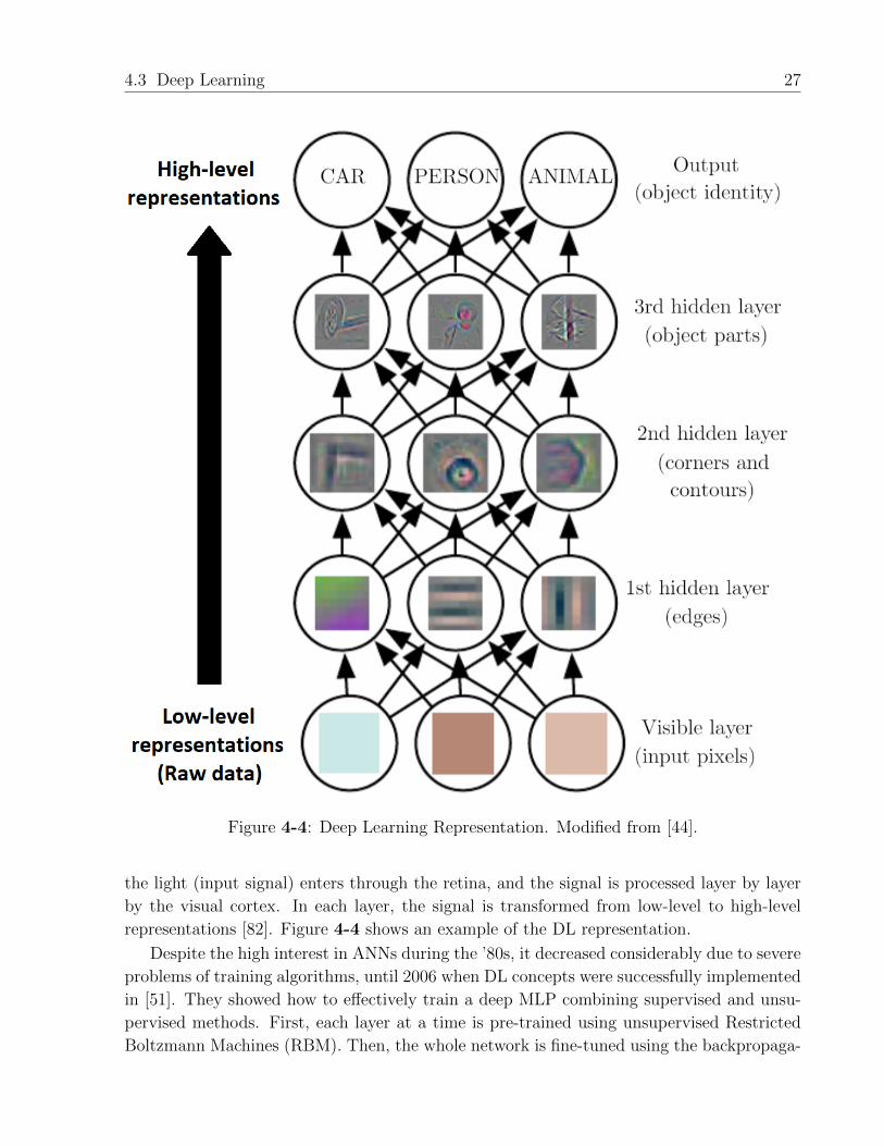
Figure 4-4: Deep Learning Representation. Modified from [44].
the light (input signal) enters through the retina, and the signal is processed layer by layer
by the visual cortex. In each layer, the signal is transformed from low-level to high-level
representations [82]. Figure 4-4 shows an example of the DL representation.
Despite the high interest in ANNs during the ’80s, it decreased considerably due to severe
problems of training algorithms, until 2006 when DL concepts were successfully implemented
in [51]. They showed how to effectively train a deep MLP combining supervised and unsu-
pervised methods. First, each layer at a time is pre-trained using unsupervised Restricted
Boltzmann Machines (RBM). Then, the whole network is fine-tuned using the backpropaga-
28 CHAPTER 4. DEEP NEURAL NETWORKS
RNN
xt
ht
RNN RNN RNN
x0
h0
x1
h1
xt
ht
Figure 4-5: An Unrolled Recurrent Neural Network.
tion algorithm. In this way, the training algorithm converges numerically, and a deep MLP
can learn complex patterns by generalizing hierarchical and sparse representations of data.
The DL “Big-Bang” started in 2009, thanks to the advances in hardware, specifically
in Graphics Processing Units (GPUs) [56]. GPUs are suitable for linear algebra operations
involved in training algorithms. Hence, the use of GPUs increased the speed of training deep-
learning model by more than 100 times [89, 13]. Even this difference has been increased more
by the recent advances in GPUs.
DL models have demonstrated greater effectiveness in several tasks (classification and
prediction) in different domains such as video analysis, audio recognition, text analysis, and
image processing. Currently, DL is a hot topic of public interest because it has faced and
solved many problems like text translation, speech recognition, motion tracking, machine
failure prediction, among others. DL has revolutionized every aspect of our daily life. Despite
its advantages, DL applications in computational finance are still limited [10, 20, 33, 102,
113, 107].
4.4 Recurrent Neural Networks
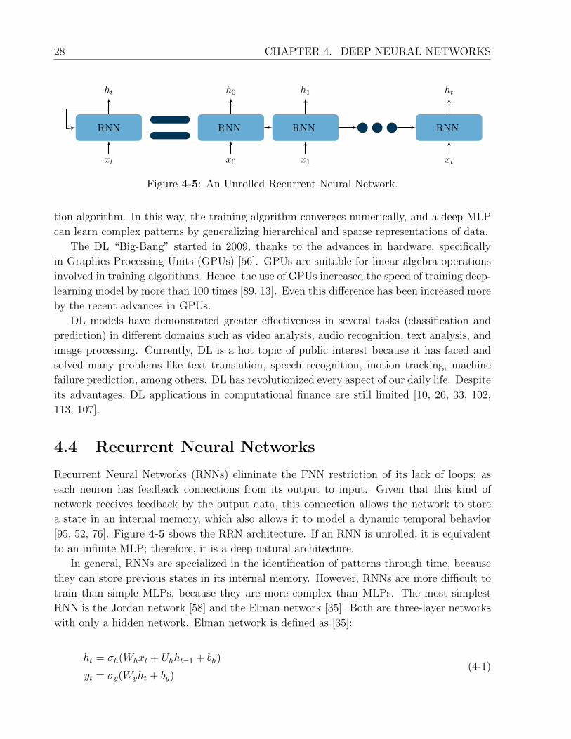
Recurrent Neural Networks (RNNs) eliminate the FNN restriction of its lack of loops; as
each neuron has feedback connections from its output to input. Given that this kind of
network receives feedback by the output data, this connection allows the network to store
a state in an internal memory, which also allows it to model a dynamic temporal behavior
[95, 52, 76]. Figure 4-5 shows the RRN architecture. If an RNN is unrolled, it is equivalent
to an infinite MLP; therefore, it is a deep natural architecture.
In general, RNNs are specialized in the identification of patterns through time, because
they can store previous states in its internal memory. However, RNNs are more difficult to
train than simple MLPs, because they are more complex than MLPs. The most simplest
RNN is the Jordan network [58] and the Elman network [35]. Both are three-layer networks
with only a hidden network. Elman network is defined as [35]:
ht = σh(Whxt + Uhht−1 + bh)
yt = σy(Wyht + by)(4-1)

4.4 Recurrent Neural Networks 29
whereas, Jordan network is defined as [58]:
ht = σh(Whxt + Uhyt−1 + bh)
yt = σy(Wyht + by)(4-2)
where xt, ht and yt are the input, hidden layer and output vectors, respectively. W and
U are the network weights matrices; b is the biases vector; and finally, σh and σy are the
activation functions.
Unfortunately, these networks have some issues related to learning too long-term time de-
pendencies and vanishing and exploding gradient problems. As a result, training algorithms
were not able to converge numerically. In 1997, the Long Short-Term Memory (LSTM),
a kind of RNN, was proposed in [52] and solved some issues of traditional RNN. LSTMs
are capable of learning in a balanced way both long and short-term dependencies [44]. A
common LSTM unit is composed of a cell and three gates (an input, output and forget gate)
[95].
ft = σg(Wfxt + Ufht−1 + bf )
it = σg(Wixt + Uiht−1 + bi)
ct = σh(Wcxt + Ucht−1 + bc)
ot = σg(Woxt + Uoht−1 + bo)
ct =
0 t = 0
ft ct−1 + it ct otherwise
ht =
0 t = 0
ot σh(ct) otherwise
(4-3)
where xt and ht are the input and output vectors, respectively. ft, it and ot are the forget,
input and output gate activation vectors, respectively. ct is the cell state vector. σg and σhare a sigmoid function and a hyperbolic tangent, respectively. The operator denotes the
Hadamard product and finally, W , U and b are parameter matrices and vectors. Figure 4-6
presents the LSTM architecture.
Additionally, models that stack multiple LSTM are more effective and successful for
specific tasks such as automatic language translation, because the process of stacking involves
applying the concept of DL. The multiple LSTM can make a better representation of the
input data, resulting in the learning of high-level representations. The first known application
of an LSTM in finance, “A LSTM-based method for stock returns prediction: A Case Study
of China Stock Market”, was published in [22].
In 2014, an LSTM variation, called Gated Recurrent Unit (GRU), was proposed in [24].
A GRU, which is a gating mechanism in RNNs, is simpler and easier to train than LSTM
because it has fewer parameters to be trained than an LSTM. A GRU combines and unifies

30 CHAPTER 4. DEEP NEURAL NETWORKS
LSTM LSTM
ht−1 ht ht+1xt−1 xt xt+1
F I C O
+
σhftit ct
ot
ct−1ct
Figure 4-6: LSTM Architecture
GRU GRU
ht−1 ht ht+1xt−1 xt xt+1
HRZ
1−
+
rtzt
ht
Figure 4-7: GRU Architecture
some LSTM gates and is defined as:
zt = σg(Wzxt + Uzht−1 + bz)
rt = σg(Wrxt + Urht−1 + br)
ht = σh(Whxt + Uh(rt ht−1) + bh)
ht =
0 t = 0
(1− zt) ht−1 + zt ht otherwise
(4-4)
where xt and ht are the input and output vectors, respectively. zt and rt are the update
and reset gate activation vectors, respectively. σg and σh are the sigmoid function and the
hyperbolic tangent function, respectively. The operator denotes the Hadamard product
and, finally, W , U and b are parameter matrices and vectors. Figure 4-7 presents the GRU
architecture.
4.5 Artificial Neural Networks in Finance
Given these characteristics, DL has emerged as a useful technique for asset price modeling
because it has proven to be able to learn complex representations of high-dimensional data.

4.5 Artificial Neural Networks in Finance 31
Table 4-1: Artificial Neural Networks Applications in Finance
Year Applications Techniques
1988 [111] Feedforward Neural Network
1990 [59] Recurrent Neural Network
1996 [104] Recurrent Neural Network
1998[85] Feedforward Neural Network + Fuzzy Inference System
[93] Recurrent and Probabilistic Neural Networks
2000 [16, 67] Multilayered Feedforward Neural Network
2001
[116] Feedforward Neural Network + Wavelet Transforms
[106] Recurrent Neural Networks + GARCH
[34] Feedforward Neural Network
2002 [63] Neuro-Fuzzy Network
2004 [21] Feedforward Artificial Neural Network
2005[9, 64] Feedforward Artificial Neural Network
[114] Recurrent Neural Network + EGARCH
2006 [81] Feedforward Neural Network
2007 [61] Recurrent Neural Network
2009 [19, 6] Feedforward Artificial Neural Network + Genetic Algorithm
2011 [55, 60] Recurrent Neural Network
2012 [109] Recurrent Neural Network
2013[27] Deep Neural Network
[36] Artificial Neural Networks + Genetic Algorithms
2014[118] Deep Belief Networks
2015[33] Convolutional Neural Network
[22] Long Short-Term Memory
2016
[31] Convolutional Neural Networks + Long Short-Term Memory
[7] Deep Neural Network
[99] Recurrent Neural Network + PCA
2017 [12] Long Short-Term Memory + Autoenconders
2018 [39] Long Short-Term Memory
32 CHAPTER 4. DEEP NEURAL NETWORKS
On DL arena, the most simple architecture is MLP, but it has demonstrated significant
results in [7, 8]. Table 4-1 presents some successful works using ANN for FTS classification
and prediction. However, the number of related works is limited. As a result, the industry
of algorithmic trading needs better models to predict price trends with greater accuracy and
precision, since market dynamics exhibit complex and stochastic behavior.
During the last years, the number of works has increased thanks to the advances in data
processing and the accessibility to financial data. It is important to remember that financial
data are costly and difficult to obtain.
Furthermore, the tick-by-tick is largely composed of many transactions at the same price
and few ones with small changes (price jumps) under normal market conditions. Those
changes, which occur without high variance, have a step-style; prices change intermittently
between two prices (the best bid and best ask quotes). Wavelets like the Haar filter (the
simplest orthogonal wavelet), can exploit this property because they are ideal for modeling
this kind of behavior. This work focuses on Deep Neural Networks (DNNs) like deep MLPs
and RNNs, which are the most widely used techniques in DL. Wavelets, in conjunction with
DNNs, allow improving the stock prices predictions on HF data concerning previous results
achieved in our previous work: [8, 7]. In the next chapter, we will present the proposed
model that uses wavelets as an input feature generator.
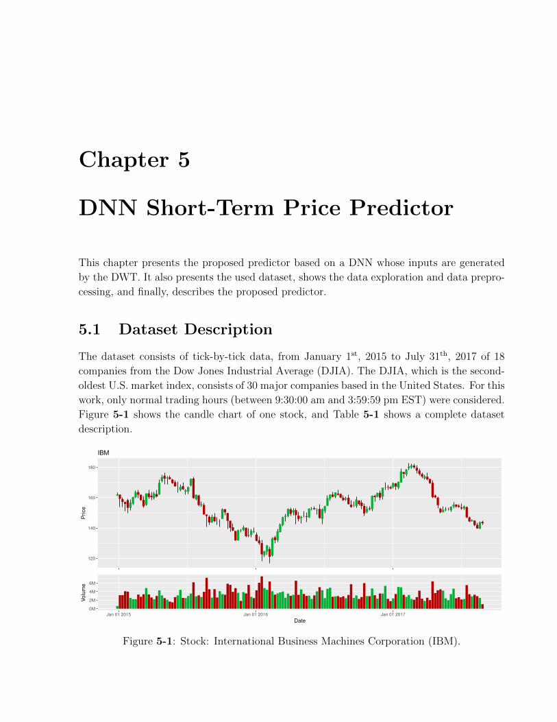
Chapter 5
DNN Short-Term Price Predictor
This chapter presents the proposed predictor based on a DNN whose inputs are generated
by the DWT. It also presents the used dataset, shows the data exploration and data prepro-
cessing, and finally, describes the proposed predictor.
5.1 Dataset Description
The dataset consists of tick-by-tick data, from January 1st, 2015 to July 31th, 2017 of 18
companies from the Dow Jones Industrial Average (DJIA). The DJIA, which is the second-
oldest U.S. market index, consists of 30 major companies based in the United States. For this
work, only normal trading hours (between 9:30:00 am and 3:59:59 pm EST) were considered.
Figure 5-1 shows the candle chart of one stock, and Table 5-1 shows a complete dataset
description.
120
140
160
180
Pri
ce
IBM
0M
2M
4M
6M
Jan 01 2015 Jan 01 2016 Jan 01 2017
Date
Volu
me
Figure 5-1: Stock: International Business Machines Corporation (IBM).
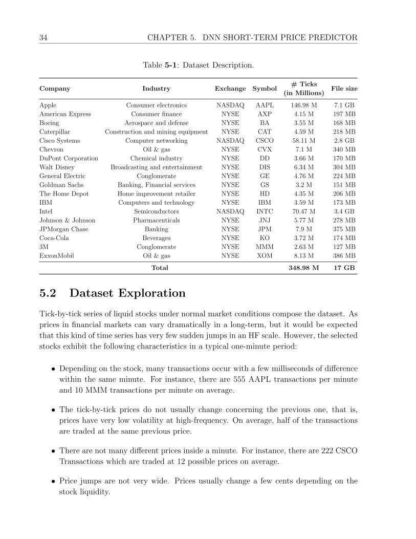
34 CHAPTER 5. DNN SHORT-TERM PRICE PREDICTOR
Table 5-1: Dataset Description.
Company Industry Exchange Symbol# Ticks
(in Millions)File size
Apple Consumer electronics NASDAQ AAPL 146.98 M 7.1 GB
American Express Consumer finance NYSE AXP 4.15 M 197 MB
Boeing Aerospace and defense NYSE BA 3.55 M 168 MB
Caterpillar Construction and mining equipment NYSE CAT 4.59 M 218 MB
Cisco Systems Computer networking NASDAQ CSCO 58.11 M 2.8 GB
Chevron Oil & gas NYSE CVX 7.1 M 340 MB
DuPont Corporation Chemical industry NYSE DD 3.66 M 170 MB
Walt Disney Broadcasting and entertainment NYSE DIS 6.34 M 304 MB
General Electric Conglomerate NYSE GE 4.76 M 224 MB
Goldman Sachs Banking, Financial services NYSE GS 3.2 M 151 MB
The Home Depot Home improvement retailer NYSE HD 4.35 M 206 MB
IBM Computers and technology NYSE IBM 3.59 M 173 MB
Intel Semiconductors NASDAQ INTC 70.47 M 3.4 GB
Johnson & Johnson Pharmaceuticals NYSE JNJ 5.77 M 278 MB
JPMorgan Chase Banking NYSE JPM 7.9 M 375 MB
Coca-Cola Beverages NYSE KO 3.72 M 174 MB
3M Conglomerate NYSE MMM 2.63 M 127 MB
ExxonMobil Oil & gas NYSE XOM 8.13 M 386 MB
Total 348.98 M 17 GB
5.2 Dataset Exploration
Tick-by-tick series of liquid stocks under normal market conditions compose the dataset. As
prices in financial markets can vary dramatically in a long-term, but it would be expected
that this kind of time series has very few sudden jumps in an HF scale. However, the selected
stocks exhibit the following characteristics in a typical one-minute period:
• Depending on the stock, many transactions occur with a few milliseconds of difference
within the same minute. For instance, there are 555 AAPL transactions per minute
and 10 MMM transactions per minute on average.
• The tick-by-tick prices do not usually change concerning the previous one, that is,
prices have very low volatility at high-frequency. On average, half of the transactions
are traded at the same previous price.
• There are not many different prices inside a minute. For instance, there are 222 CSCO
Transactions which are traded at 12 possible prices on average.
• Price jumps are not very wide. Prices usually change a few cents depending on the
stock liquidity.
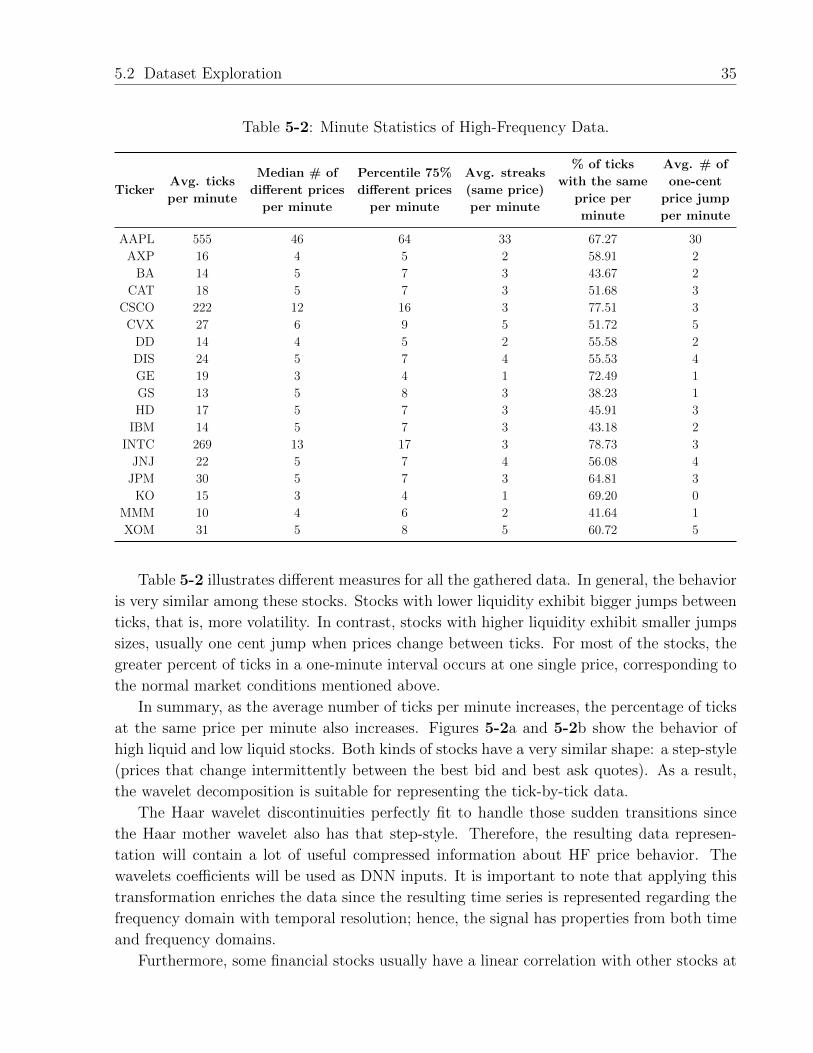
5.2 Dataset Exploration 35
Table 5-2: Minute Statistics of High-Frequency Data.
TickerAvg. ticks
per minute
Median # of
different prices
per minute
Percentile 75%
different prices
per minute
Avg. streaks
(same price)
per minute
% of ticks
with the same
price per
minute
Avg. # of
one-cent
price jump
per minute
AAPL 555 46 64 33 67.27 30
AXP 16 4 5 2 58.91 2
BA 14 5 7 3 43.67 2
CAT 18 5 7 3 51.68 3
CSCO 222 12 16 3 77.51 3
CVX 27 6 9 5 51.72 5
DD 14 4 5 2 55.58 2
DIS 24 5 7 4 55.53 4
GE 19 3 4 1 72.49 1
GS 13 5 8 3 38.23 1
HD 17 5 7 3 45.91 3
IBM 14 5 7 3 43.18 2
INTC 269 13 17 3 78.73 3
JNJ 22 5 7 4 56.08 4
JPM 30 5 7 3 64.81 3
KO 15 3 4 1 69.20 0
MMM 10 4 6 2 41.64 1
XOM 31 5 8 5 60.72 5
Table 5-2 illustrates different measures for all the gathered data. In general, the behavior
is very similar among these stocks. Stocks with lower liquidity exhibit bigger jumps between
ticks, that is, more volatility. In contrast, stocks with higher liquidity exhibit smaller jumps
sizes, usually one cent jump when prices change between ticks. For most of the stocks, the
greater percent of ticks in a one-minute interval occurs at one single price, corresponding to
the normal market conditions mentioned above.
In summary, as the average number of ticks per minute increases, the percentage of ticks
at the same price per minute also increases. Figures 5-2a and 5-2b show the behavior of
high liquid and low liquid stocks. Both kinds of stocks have a very similar shape: a step-style
(prices that change intermittently between the best bid and best ask quotes). As a result,
the wavelet decomposition is suitable for representing the tick-by-tick data.
The Haar wavelet discontinuities perfectly fit to handle those sudden transitions since
the Haar mother wavelet also has that step-style. Therefore, the resulting data represen-
tation will contain a lot of useful compressed information about HF price behavior. The
wavelets coefficients will be used as DNN inputs. It is important to note that applying this
transformation enriches the data since the resulting time series is represented regarding the
frequency domain with temporal resolution; hence, the signal has properties from both time
and frequency domains.
Furthermore, some financial stocks usually have a linear correlation with other stocks at
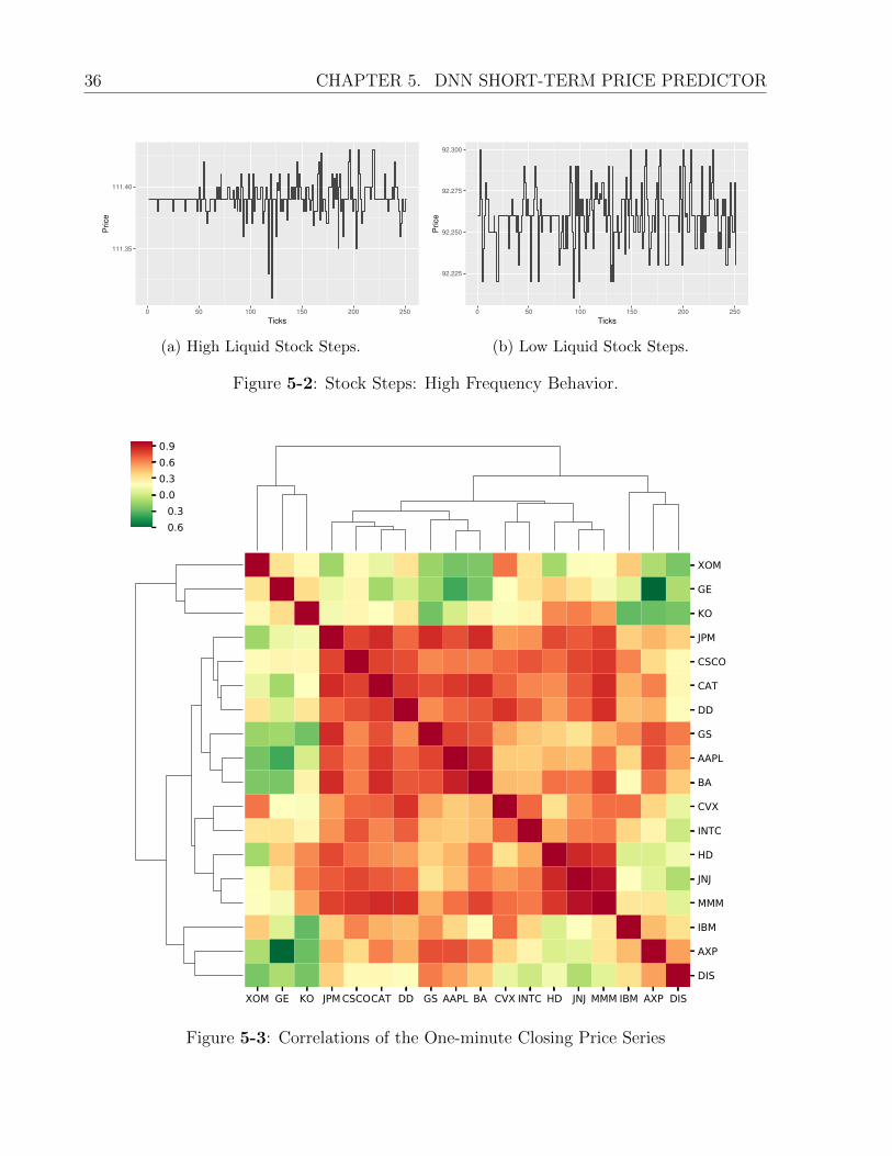
36 CHAPTER 5. DNN SHORT-TERM PRICE PREDICTOR
111.35
111.40
0 50 100 150 200 250
Ticks
Pri
ce
(a) High Liquid Stock Steps.
92.225
92.250
92.275
92.300
0 50 100 150 200 250
Ticks
Pri
ce
(b) Low Liquid Stock Steps.
Figure 5-2: Stock Steps: High Frequency Behavior.
XOM GE KO JPMCSCOCAT DD GS AAPL BA CVX INTC HD JNJ MMM IBM AXP DIS
XOM
GE
KO
JPM
CSCO
CAT
DD
GS
AAPL
BA
CVX
INTC
HD
JNJ
MMM
IBM
AXP
DIS
−0.6−0.30.00.30.60.9
Figure 5-3: Correlations of the One-minute Closing Price Series
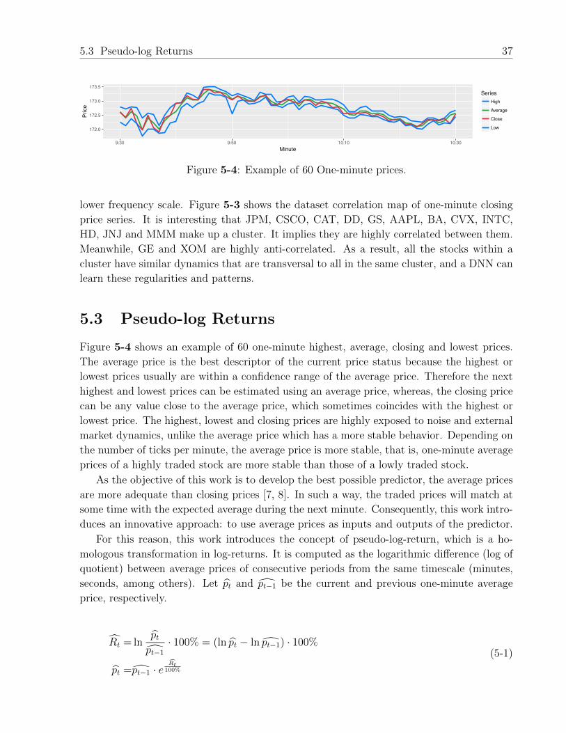
5.3 Pseudo-log Returns 37
172.0
172.5
173.0
173.5
9:30 9:50 10:10 10:30
Minute
Pri
ce
Series
High
Average
Close
Low
Figure 5-4: Example of 60 One-minute prices.
lower frequency scale. Figure 5-3 shows the dataset correlation map of one-minute closing
price series. It is interesting that JPM, CSCO, CAT, DD, GS, AAPL, BA, CVX, INTC,
HD, JNJ and MMM make up a cluster. It implies they are highly correlated between them.
Meanwhile, GE and XOM are highly anti-correlated. As a result, all the stocks within a
cluster have similar dynamics that are transversal to all in the same cluster, and a DNN can
learn these regularities and patterns.
5.3 Pseudo-log Returns
Figure 5-4 shows an example of 60 one-minute highest, average, closing and lowest prices.
The average price is the best descriptor of the current price status because the highest or
lowest prices usually are within a confidence range of the average price. Therefore the next
highest and lowest prices can be estimated using an average price, whereas, the closing price
can be any value close to the average price, which sometimes coincides with the highest or
lowest price. The highest, lowest and closing prices are highly exposed to noise and external
market dynamics, unlike the average price which has a more stable behavior. Depending on
the number of ticks per minute, the average price is more stable, that is, one-minute average
prices of a highly traded stock are more stable than those of a lowly traded stock.
As the objective of this work is to develop the best possible predictor, the average prices
are more adequate than closing prices [7, 8]. In such a way, the traded prices will match at
some time with the expected average during the next minute. Consequently, this work intro-
duces an innovative approach: to use average prices as inputs and outputs of the predictor.
For this reason, this work introduces the concept of pseudo-log-return, which is a ho-
mologous transformation in log-returns. It is computed as the logarithmic difference (log of
quotient) between average prices of consecutive periods from the same timescale (minutes,
seconds, among others). Let pt and pt−1 be the current and previous one-minute average
price, respectively.
Rt = lnptpt−1
· 100% = (ln pt − ln pt−1) · 100%
pt =pt−1 · eRt
100%
(5-1)
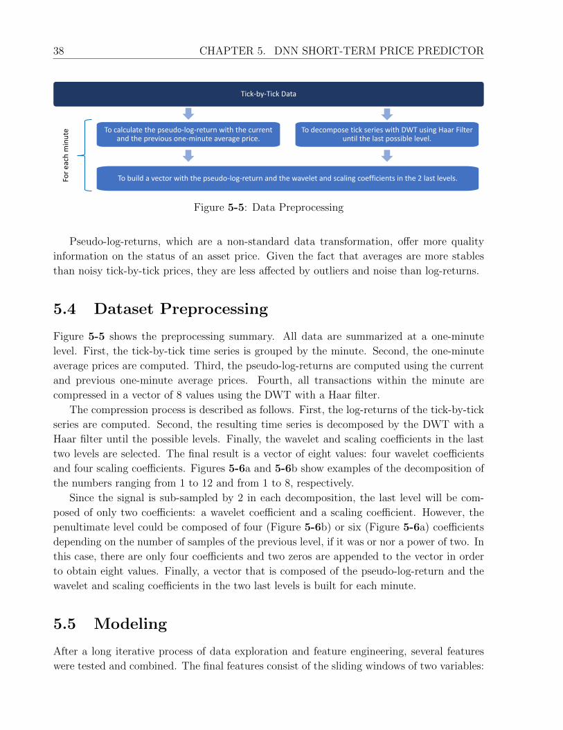
38 CHAPTER 5. DNN SHORT-TERM PRICE PREDICTOR
Tick-by-Tick Data
Fo
r e
ach
min
ute To calculate the pseudo-log-return with the current
and the previous one-minute average price.
To decompose tick series with DWT using Haar Filter
until the last possible level.
To build a vector with the pseudo-log-return and the wavelet and scaling coefficients in the 2 last levels.
Figure 5-5: Data Preprocessing
Pseudo-log-returns, which are a non-standard data transformation, offer more quality
information on the status of an asset price. Given the fact that averages are more stables
than noisy tick-by-tick prices, they are less affected by outliers and noise than log-returns.
5.4 Dataset Preprocessing
Figure 5-5 shows the preprocessing summary. All data are summarized at a one-minute
level. First, the tick-by-tick time series is grouped by the minute. Second, the one-minute
average prices are computed. Third, the pseudo-log-returns are computed using the current
and previous one-minute average prices. Fourth, all transactions within the minute are
compressed in a vector of 8 values using the DWT with a Haar filter.
The compression process is described as follows. First, the log-returns of the tick-by-tick
series are computed. Second, the resulting time series is decomposed by the DWT with a
Haar filter until the possible levels. Finally, the wavelet and scaling coefficients in the last
two levels are selected. The final result is a vector of eight values: four wavelet coefficients
and four scaling coefficients. Figures 5-6a and 5-6b show examples of the decomposition of
the numbers ranging from 1 to 12 and from 1 to 8, respectively.
Since the signal is sub-sampled by 2 in each decomposition, the last level will be com-
posed of only two coefficients: a wavelet coefficient and a scaling coefficient. However, the
penultimate level could be composed of four (Figure 5-6b) or six (Figure 5-6a) coefficients
depending on the number of samples of the previous level, if it was or nor a power of two. In
this case, there are only four coefficients and two zeros are appended to the vector in order
to obtain eight values. Finally, a vector that is composed of the pseudo-log-return and the
wavelet and scaling coefficients in the two last levels is built for each minute.
5.5 Modeling
After a long iterative process of data exploration and feature engineering, several features
were tested and combined. The final features consist of the sliding windows of two variables:

5.5 Modeling 39
Wavelet Coefficients W
5.656854
2
0,7071068 0,7071068
2
0.7071068 0,7071068
2
0,7071068 0.7071068
Scaling coefficients V
24.04163
5
2.121320 4.949747
13
7.778175 10.606602
21
13.435029 16.263456
5,656854 2 2 2 24.04163 5 13 21
A compressed time series: a vector (1x8)
Level 1
Level 2
Level 3
1 2 3 4 5 6 7 8 9 10 11 12Signal
DW
T D
eco
mp
osi
tio
n
(a) Case I.
Wavelet Coefficients W
5.656854
2
0,7071068 0,7071068
2
0.7071068 0,7071068
Scaling coefficients V
12.72792
5
2.121320 4.949747
13
7.778175 10.606602
5.656854 2 2 0 12.72792 5 13 0
A compressed time series: a vector (1x8)
Level 1
Level 2
Level 3
1 2 3 4 5 6 7 8Signal
DW
T D
eco
mp
osi
tio
n
(b) Case II.
Figure 5-6: Compressed Tick-by-Tick Series using DWT.
one-minute pseudo-log-returns and one-minute compressed tick-by-tick vectors with length
8. Each vector is the result of transforming tick-by-tick transactions recorded in a particular
minute using a DWT and a Haar filter. Several DNN architectures will be tested in Chapter
7. The used degrees of freedom were the number of previous observations (sliding window
size from 2 to 60 minutes), number of layers (from 1 to 10), number of neurons per layer and
type of activation function (Tanh, Maxout, Rectifier).
The final architecture was chosen taking account the balance between efficiency and
accuracy. Figure 5-7 shows the network architecture sketch with five hidden layers (27, 22,
17, 11 and 6 neurons using Tanh activation function, respectively) and a window size of 3.
Chapter 7 will show a comparison between the proposed DNN, the Auto-regressive Inte-
grated Moving Average (ARIMA) model, three different alternatives of DNN architectures,
a Random Walk (RW) simulation, and other seven classic machine learning techniques of
similar complexity.

40 CHAPTER 5. DNN SHORT-TERM PRICE PREDICTOR
tt-1
t-2
Pseu
do-log-retu
rnW
avelet
coeffi
cients
[1..4]
Scalin
g
coeffi
cients
[1..4]
Pseu
do-log-retu
rnW
avelet
coeffi
cients
[1..4]
Scalin
g
coeffi
cients
[1..4]
Pseu
do-log-retu
rnW
avelet
coeffi
cients
[1..4]
Scalin
g
coeffi
cients
[1..4]
Pseu
do-log-retu
rn
t+1
Pred
ictedA
verage
Price
t+1
Input
Layer
Hid
den
Layer
1
Hid
den
Layer
2
Hid
den
Layer
3
Hid
den
Layer
4
Hid
den
Layer
5
Outp
ut
Layer
Figu
re5-7
:D
eepA
rchitectu
re.

Chapter 6
High-Frequency Strategy
This chapter presents the proposed high-frequency trading strategy that the described short-
term price predictor will use. This strategy consists of a variation of one presented in our
previous work [7, 8].
6.1 Baseline Strategy
A high-frequency trading strategy based on a DNN, which predicts the next one-minute
average price, was proposed in [7, 8]. It was tested over the AAPL stock during the financial
crisis of 2008 and yielded extraordinary profits. Figure 6-1 shows the strategy flowchart.
This strategy operates at high-frequency time scale. It opens a position at the beginning
of each minute according to the price target (the predicted one-minute average price) and
closes the position when the price reaches the target at any moment or when the minute ends
(in case of the price never yields the target price). It opens the position in the following way:
If the next predicted average price is above/below the last closing price, it always buys/sells
a stock. This strategy is simple but has several issues in a real environment. For instance,
it does not consider:
• Non-liquid periods: the strategy could buy at high prices or sell at low prices
during non-liquid periods because there is not enough supply or demand to trade and
get profits.
• Sharply price variations: The strategy waits until the end of the minute to close
its position in order to stop the looses. However, if the price changes sharply and
goes to the opposite side during that minute, this strategy is vulnerable to volatility
and potential losses. Besides, the strategy has an asymmetric behavior, when the
price reaches the target price, the strategy cuts the earnings. Meanwhile, when the
price never reaches the target price and goes to the wrong side, there are no stop-loss
mechanisms.

42 CHAPTER 6. HIGH-FREQUENCY STRATEGY
At the beginning of each minute and using the predicted closing price
BUY SELL
Do nothing until next minute
Close position
Have the target
price been reached or
does the minute end?
Previous
closing price <
predicted price
Previous
closing price >
predicted price
Otherwise
YesNo
Figure 6-1: Strategy Flowchart.
At the beginning of each minute and using the predicted closing price
BUY SELL
Do nothing until next minute
Close position
Have the stop-loss
or target price been
reached or does the
minute end?
Previous
closing price <
predicted price
Previous
closing price >
predicted price
Were not enough ticks
or is it 9:30 AM?Otherwise
YesNo
Figure 6-2: Modified Strategy Flowchart.

6.2 Proposed Strategy 43
• Bearish or bullish market openings: News or earnings reports, which usually are
published before market openings, have a strong impact on the markets and can make
them have a bullish or bearish expectation. Then, the strategy will operate based on
old data from the previous day and its behavior may be unexpected and risky since
data will not be reliable about the actual market status.
6.2 Proposed Strategy
This work presents a modified version of the previous strategy. Figure 6-2 shows the new
flowchart, which includes three main changes:
First, it only trades if the last minute had at least n transactions. There is no guarantee
of knowing if the next minute will be enough liquid to trade. However, under the assumption
that the last minute was liquid, then the probability that the next minute will also be enough
liquid is high. For this work, the selected criterion to determine if a minute is liquid or not
is that the amount of transactions during that minute is greater than the 25th percentile.
This threshold can be easily calculated from historical data.
Second, if the strategy opens a position and the price goes in the opposite direction and
exceeds a threshold, the strategy will close its position. For this work, the threshold was
defined as the current price minus the distance from the target price to the current price. For
example, if the current price is $1000 and the target price is $1001, the stop-loss price will
be $999. Meanwhile, if the current price is $1000 and the target price is $999, the stop-loss
price will be $1001. In consequence, the strategy becomes symmetric.
And finally, it does not trade on the first minute of the day. Thereby, the strategy avoids
volatility and risks associated with market openings.
6.3 Simulation of the Proposed Strategy
Those changes have a high impact on the performance of the strategies. Figure 6-3 shows
the old strategy performance compared to the new strategy performance during a trading
simulation using the same testing period from the previous chapter (approximately five
months). This simulation did not take into account transaction and spread costs. For each
stock, it starts with 1 dollar and reinvests all the available money in the following operations.
The accumulated profits varied a lot: the new strategy had a positive profit, contrary
to the old strategy. On average, the old strategy made a lot of good trades (%65), but it
lost too much money (until -2% per operation) on a few others. The left histogram shows
an asymmetric behavior and the right one shows a symmetric-like behavior. It is evident
that the stop-loss mechanism implemented by the new strategy had a positive effect on its
performance. Furthermore, the charts on the last row show that the old strategy lost too
much money (until -2% on average) during the first minute of the day. As a result, it proves

44 CHAPTER 6. HIGH-FREQUENCY STRATEGY
−0.04
−0.02
0.00
Apr 01 2017 May 01 2017 Jun 01 2017 Jul 01 2017 Aug 01 2017 Sep 01 2017
Date
Pro
fit
Profits
−0.4
−0.3
−0.2
−0.1
0.0
Apr 01 2017 May 01 2017 Jun 01 2017 Jul 01 2017 Aug 01 2017 Sep 01 2017
Date
Pro
fit
Accumulated profits
Trades
Earnings (25448 ~ 65.4%)
Losses (11024 ~ 28.3%)
None (2455 ~ 6.3%)
Trades
0
5000
10000
15000
−1e−03 −5e−04 0e+00 5e−04 1e−03
Profit
Count
Histogram of profits per position
0
100
200
300
400
Apr 01 2017 May 01 2017 Jun 01 2017 Jul 01 2017 Aug 01 2017 Sep 01 2017
Date
Count
Position
Buy
Sell
Stay
Positions
0%
25%
50%
75%
100%
Apr 01 2017 May 01 2017 Jun 01 2017 Jul 01 2017 Aug 01 2017 Sep 01 2017
Date
Count
Trades
Earnings
Losses
None
Trades per Day
−0.020
−0.015
−0.010
−0.005
0.000
0.005
10:00 12:00 14:00 16:00
Time
Pro
fit
Profits per minute of the day
(a) Old Strategy
−0.005
0.000
0.005
Apr 01 2017 May 01 2017 Jun 01 2017 Jul 01 2017 Aug 01 2017 Sep 01 2017
Date
Pro
fit
Profits
0.00
0.02
0.04
0.06
Apr 01 2017 May 01 2017 Jun 01 2017 Jul 01 2017 Aug 01 2017 Sep 01 2017
Date
Pro
fit
Accumulated profits
Trades
Earnings (13679 ~ 50.1%)
Losses (13278 ~ 48.6%)
None (373 ~ 1.4%)
Trades
0
2000
4000
6000
8000
−0.00050 −0.00025 0.00000 0.00025 0.00050
Profit
Count
Histogram of profits per position
0
100
200
300
400
Apr 01 2017 May 01 2017 Jun 01 2017 Jul 01 2017 Aug 01 2017 Sep 01 2017
Date
Count
Position
Buy
Sell
Stay
Positions
0%
25%
50%
75%
100%
Apr 01 2017 May 01 2017 Jun 01 2017 Jul 01 2017 Aug 01 2017 Sep 01 2017
Date
Count
Trades
Earnings
Losses
None
Trades per Day
−4e−06
0e+00
4e−06
8e−06
10:00 12:00 14:00 16:00
Time
Pro
fit
Profits per minute of the day
(b) New Strategy
Figure 6-3: Performance Comparison of the Strategies: The Walt Disney Company (DIS).
that refraining from trading during the market opening can avoid potential losses and also
reduces exposure to risk. Moreover, Chapter 7 will show a comparison between the proposed
HF trading strategy and three types of trading strategies: A Buy & Hold Strategy, an RSI
Strategy with six different time windows, and a one-minute Random Trading Strategy.

Chapter 7
Experiments and Results
This chapter presents the experimental setting and the corresponding results of the proposed
DNN short-term price predictor and the proposed high-frequency trading strategy.
7.1 Experimental Setting: Short-Term Price Predictor
Table 7-1 shows the experimental setting overview for testing the proposed short-term pre-
dictor and for comparing it against different DNN architectures, classical econometric and
statistical models (ARIMA and RW) and classical machine learning techniques (Linear re-
gression, Ridge, Lasso, Bayesian ridge, SGD regressor, Decision trees, and SVR). The fol-
lowing subsections present the proposed experiments in more detail.
Multi-Layer Perceptron
In [7, 8], a MLP was proposed. It also predicts the next one-minute pseudo-log-return. Its
input features are 3n+ 2 values: the current time (hour and minute), the last n one-minute
pseudo-log-returns, the last n one-minute standard deviations of prices and the last n one-
minute trend indicators, where n is the window size. The trend indicator is calculated as
the slope a of a fitted linear model on tick-by-tick prices within the same minute.
The DNN has one input layer, L hidden layers, and one output layer. The number of
neurons in each layer depends on the input number I as well as on hidden layers number
L. In each hidden layer, the number of neurons decreases with a constant factor of 1L
. For
example, with five hidden layers: Each layer will have I, d45Ie, d3
5Ie, d2
5Ie, d1
5Ie neurons
respectively. For example, with three hidden layers: Each layer will have I, d23Ie, d1
3Ie
respectively. The output layer always has one neuron. All neurons in hidden layers use a
Tanh activation function, whereas the output neuron uses a Linear activation function.
Several MLPs architectures were tested. The used degrees of freedom were the number of
previous observations (sliding window size from 2 to 60 minutes), number of layers (from 2 to
10), number of neurons per layer, type of activation function (Tanh, Maxout, Rectifier). The

46 CHAPTER 7. EXPERIMENTS AND RESULTS
Table 7-1: Experimental Setting: Short-Term Price Predictor
Technique InputsExplored Freedom Degrees
Window Size Hidden Layers
Multi-Layer
Perceptron
1. Time (Hour and Minute)
2. One-minute pseudo re-
turn.
3. One-minute standard de-
viation.
4. Trend indicator.
2 - 60 2 - 10
ARIMA 1. One-minute pseudo re-
turns
1 - 5 NA
RW NA NA
Multi-Layer
Perceptron
+ DWT
1. One-minute pseudo re-
turn.
2. Compressed tick-by-tick
time series by DWT.
2 - 60
2 - 10
LSTM + DWT
GRU + DWT
Linear Regression
NA
Ridge
Lasso
Bayesian Ridge
SGD Regressor
Decision Trees
SVR
final architecture was chosen taking account the balance between efficiency and accuracy.
Let n be 3 and the architecture be composed of 5 hidden layers, and each layer with 11, 8,
7, 5, 3 neurons, respectively. In each hidden layer, the number of neurons decreases with a
constant factor of 15.
H2O, which is open-source software for big-data analysis, was used to train the MLPs.
The ADADELTA training method was selected because it offers several benefits. Given that
ADADELTA is a per-dimension adaptive learning rate method for gradient descent, it is
not necessary to manually search parameters for gradient descent and is also robust to large
gradients and noise. The chosen ADADELTA parameters were ρ = 0.9999 and ε = 10−9.
The MLPs were trained during 50 epochs.
ARIMA
ARIMA is the most used analytic technique for forecasting financial time series. Even though
it has good performance over in-sample datasets, it has bad performance over out-sample
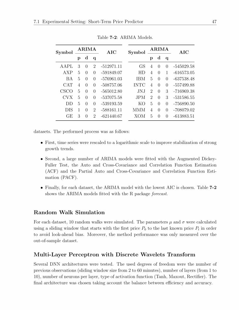
7.1 Experimental Setting: Short-Term Price Predictor 47
Table 7-2: ARIMA Models.
SymbolARIMA
AICp d q
AAPL 3 0 2 -512971.11
AXP 5 0 0 -591849.07
BA 5 0 0 -576961.03
CAT 4 0 0 -508757.06
CSCO 5 0 0 -565012.80
CVX 5 0 0 -537075.58
DD 5 0 0 -539193.59
DIS 1 0 2 -588161.11
GE 3 0 2 -621440.67
SymbolARIMA
AICp d q
GS 4 0 0 -545029.58
HD 4 0 1 -616573.05
IBM 5 0 0 -637538.48
INTC 4 0 0 -557499.88
JNJ 2 0 3 -716969.38
JPM 2 0 3 -531586.55
KO 5 0 0 -756890.50
MMM 4 0 0 -708079.02
XOM 5 0 0 -613883.51
datasets. The performed process was as follows:
• First, time series were rescaled to a logarithmic scale to improve stabilization of strong
growth trends.
• Second, a large number of ARIMA models were fitted with the Augmented Dickey-
Fuller Test, the Auto and Cross-Covariance and Correlation Function Estimation
(ACF) and the Partial Auto and Cross-Covariance and Correlation Function Esti-
mation (PACF).
• Finally, for each dataset, the ARIMA model with the lowest AIC is chosen. Table 7-2
shows the ARIMA models fitted with the R package forecast.
Random Walk Simulation
For each dataset, 10 random walks were simulated. The parameters µ and σ were calculated
using a sliding window that starts with the first price P0 to the last known price Pt in order
to avoid look-ahead bias. Moreover, the method performance was only measured over the
out-of-sample dataset.
Multi-Layer Perceptron with Discrete Wavelets Transform
Several DNN architectures were tested. The used degrees of freedom were the number of
previous observations (sliding window size from 2 to 60 minutes), number of layers (from 1 to
10), number of neurons per layer, type of activation function (Tanh, Maxout, Rectifier). The
final architecture was chosen taking account the balance between efficiency and accuracy.

48 CHAPTER 7. EXPERIMENTS AND RESULTS
In summary, the selected features are the one-minute pseudo-log-returns and the com-
pressed tick-by-tick time series (8 values per minute). The selected sliding window size is
3. Therefore, the network input is a vector of 27 values, whereas, the network output is the
next one-minute pseudo-log-return. Moreover, the final architecture has one input layer, five
hidden layers (27, 22, 17, 11 and 6 neurons using Tanh activation function, respectively)
and one output layer (1 neuron using Linear activation function). The number of neurons
in each layer decreases with a constant factor of 15.
TensorFlow, an open-source machine learning framework, was used to train the MLPs.
Adam optimization was selected. The mean squared error was chosen as the loss function.
The default parameters were used for the training process. The MLPs were trained during
200 epochs.
Recurrent Neural Networks with Discrete Wavelets Transform
Furthermore, a GRU and an LSTM were trained using the same proposed method inputs
(the last three one-minute pseudo-log-returns and the last three compressed tick-by-tick time
series (8 × 3)) and the same proposed method’s output (the next one-minute pseudo-log-
return). All neurons use a tanh activation function, except the output neuron which uses a
linear function. Each architecture only has five hidden layers in order to reduce the model’s
complexity and decrease training times. Therefore, each hidden layer is composed of 27, 22,
17, 11 and 6 units. The number of neurons decreases with a constant factor of 15.
TensorFlow was also used to train the RNNs. Adam optimization was selected. The
mean squared error was chosen as the loss function. The default parameters were used for
the training process. The RNNs were trained during 200 epochs.
Classic Statistical and Machine Learning Techniques
In order to make a more robust benchmark that compares the results with another approach
of similar complexity. The following seven statistical and machine learning techniques for
regression were trained:
Linear Models
They model the output like a linear combination of the inputs variables.
y(w, x) = w0 + w1x1 + · · ·+ wpxp (7-1)
• Linear Regression: It fits by minimizing the residual sum of squares between the
observed outputs and the linear approximation predictions.
minw||Xw − y||22 (7-2)

7.2 Experiment and Results: Price Predictor 49
• Ridge: It imposes a penalty on the size of coefficients.
minw||Xw − y||22 + α||w||22 (7-3)
• Lasso: It imposes a penalty on the size of coefficients.
minw
1
2nsamples||Xw − y||22 + α||w||21 (7-4)
• Bayesian Ridge: It estimates a probabilistic model within the context of Bayesian
inference.
• SGD Regressor: It fits by minimizing a regularized empirical loss with Stochastic
Gradient Descent (SGD).
Decision Trees
They are one of the favorite supervised machine learning techniques. The Decision Trees,
which are commonly used for classification and regression problems, infers a set of simple
decisions rules from the variable inputs.
SVR
The Support Vector Regression (SVR) is a supervised machine learning technique based on
Support Vector Machines (SVM). They construct a set of hyperplanes in a high-dimensional
space that segments the space. Although they are a powerful technique, they do not scale
well with large datasets.
The chosen input variables were the last n observations (one-minute pseudo-log-returns),
and the output variable was the next one-minute pseudo-log-return. The explored window
sizes n were 2, 3, 4, 5, 6, 7, 8, 9, 10, 15, 30 and 60. These models were trained with the
Python library scikit-learn using the default parameters.
7.2 Experiment and Results: Price Predictor
Each dataset described in the previous section was preprocessed and divided into two parts:
first 85% is an in-sample dataset, and the remaining 15% is an out-sample dataset. For each
symbol and ANN model, ten ANNs were trained, and then the average error was computed
and reported. Overall, all the model results were homogeneous and stable.
Figure 7-2 shows the Performance of DNN vs. ARIMA and RW. After seeing the perfor-
mance of the models over the out-sample datasets, machine learning techniques had a much
better performance compared to ARIMA and Random Walks. The superiority of DNNs is
clear over traditional and theoretical methods such as ARIMA and RW. Figures 7-1a and

50 CHAPTER 7. EXPERIMENTS AND RESULTS
45
50
55
BayesianRidge
DecisionTree
Lasso LinearRegression
Ridge SGD SVR
Model
DA
(%
)
(a) DA per Model.
45
50
55
2 3 4 5 6 7 8 9 10 15 30 60
n
DA
(%
)
(b) DA per Window Size (n).
Figure 7-1: Performance of the Classic Statistical and Machine Learning Techniques.
DA
Training
DA
Testing
MSE
Training
MSE
Testing
ARIMAMLP MLP + DWT
GRU + DWT
LSTM + DWT
ARIMAMLP MLP + DWT
GRU + DWT
LSTM + DWT
RW
ARIMAMLP MLP + DWT
GRU + DWT
LSTM + DWT
ARIMAMLP MLP + DWT
GRU + DWT
LSTM + DWT
RW0.000
0.005
0.010
0.015
0.020
0
20
40
60
0.002
0.003
0.004
0.005
0.006
55
60
65
70
Model
Perf
orm
ance
Figure 7-2: Deep Neural Networks vs. ARIMA and Random Walk.
7-1b show the seven techniques performance. The DA achieved during the testing phase by
these techniques ranges from 45.34% to 58.42%. Although these techniques are approaches
with similar complexity like DNNs, they are not able to compete with the proposed model
that uses the power of the wavelets decomposition and the DL paradigm.
Figure 7-3 shows the performance of the DNNs. Meanwhile, networks using DWT are
slightly better than the one without DWT; On average, MLP without DWT, MLP with
DWT, GRU with DWT and LSTM with DWT achieved an MSE of 0.002026, 0.001963,
0.001941, 0.001939 and a DA of 65.27%, 67.38%, 67.74%, 67.72%, respectively. In contrast,
ARIMA achieved an MSE of 0.002287 and a DA of 12.48%, RW achieved an MSE of 0.01271
and a DA of 49.26%. The best model was GRU, though its performance is almost equal
to LSTM. Figure 7-4 shows the performance of the models per symbol during the training
and testing phases. During the testing phase, the best symbol was APPL (DA=71.98% -

7.2 Experiment and Results: Price Predictor 51
DA
Training
DA
Testing
MSE
Training
MSE
Testing
MLP MLP + DWT
GRU + DWT
LSTM + DWT
MLP MLP + DWT
GRU + DWT
LSTM + DWT
0.001
0.002
0.003
0.004
62.5
65.0
67.5
70.0
72.5
0.002
0.003
0.004
0.005
65.0
67.5
70.0
Model
Perf
orm
ance
Figure 7-3: Performance of the Deep Neural Networks.
AAPL AXP BA CAT CSCO CVX DD DIS GE GS HD IBM INTC JNJ JPM KO MMM XOM
MS
ED
A
Tra
inin
g
Testing
Tra
inin
g
Testing
Tra
inin
g
Testing
Tra
inin
g
Testing
Tra
inin
g
Testing
Tra
inin
g
Testing
Tra
inin
g
Testing
Tra
inin
g
Testing
Tra
inin
g
Testing
Tra
inin
g
Testing
Tra
inin
g
Testing
Tra
inin
g
Testing
Tra
inin
g
Testing
Tra
inin
g
Testing
Tra
inin
g
Testing
Tra
inin
g
Testing
Tra
inin
g
Testing
Tra
inin
g
Testing
0.001
0.002
0.003
0.004
0.005
62.5
65.0
67.5
70.0
72.5
Type
Perf
orm
ance
Model MLP MLP + DWT LSTM + DWT GRU + DWT
Figure 7-4: Model Performance per Symbol during the Training and Testing Phases
MSE=0.0027), and the worst was MMM (DA=64.11% - MSE=0.0010), with the model GRU
+ DWT.
In order to ensure the quality of the results, 12 Paired Student’s t-tests were carried out
with a significance level α at 0.01. Table 7-3 shows the results. It can be concluded that MLP
is better than RW and ARIMA, MLP with DWT is better than MLP, LSTM with DWT and
GRU with DWT are better than MLP with DWT, but there is not enough evidence that
GRU with DWT is better than LSTM with DWT. Otherwise, GRU is significantly better
than LSTM, though it has the same performance as LSTM, GRU has less complexity and
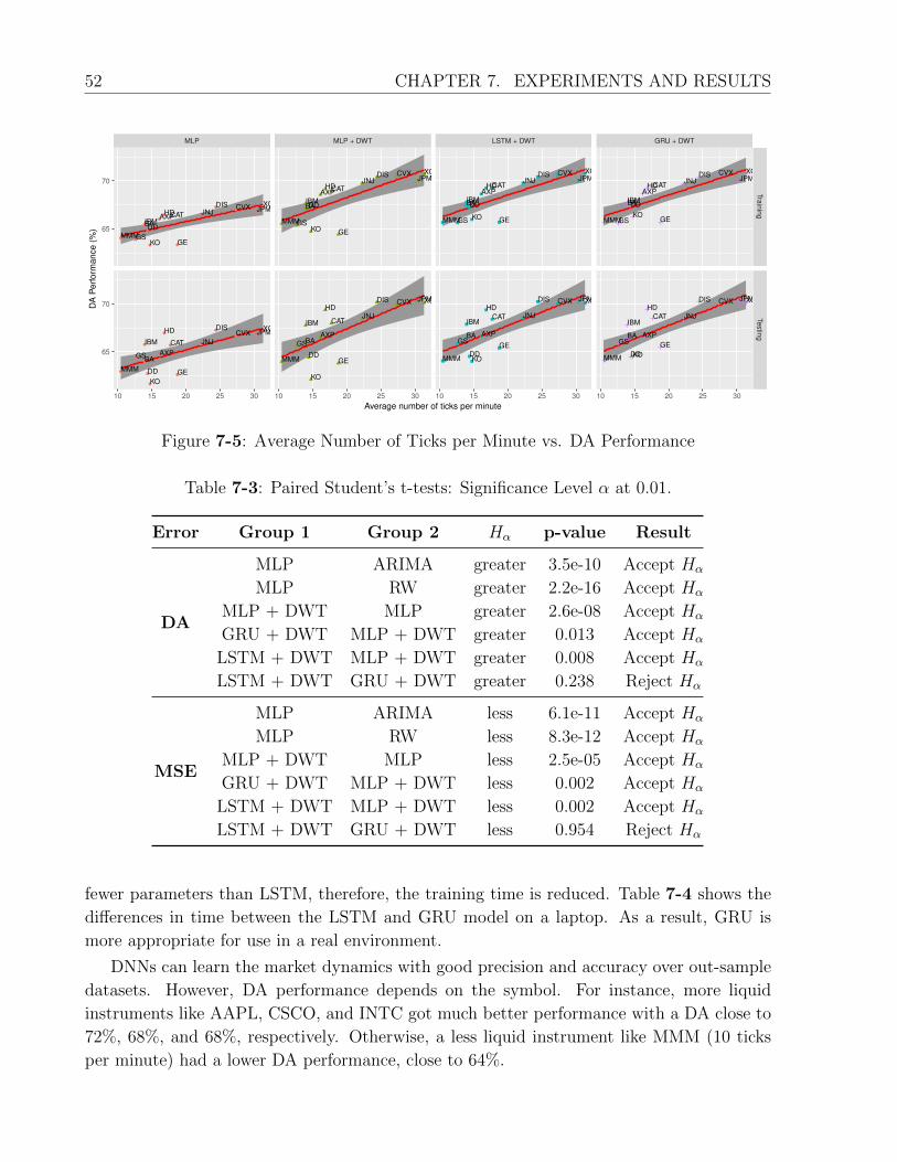
52 CHAPTER 7. EXPERIMENTS AND RESULTS
AXPBA
CATCVX
DD
DIS
GEGS
HD
IBM
JNJ JPM
KOMMM
XOM
AXPBA
CAT
CVX
DD
DIS
GE
GS
HD
IBM JNJ
JPM
KO
MMM
XOM
AXP
BA
CAT
CVX
DD
DIS
GE
GS
HD
IBM
JNJ JPM
KOMMM
XOM
AXPBA
CAT
CVX
DD
DIS
GE
GS
HD
IBMJNJ
JPM
KO
MMM
XOM
AXP
BA
CAT
CVX
DD
DIS
GEGS
HD
IBM
JNJ JPM
KOMMM
XOM
AXPBA
CAT
CVX
DD
DIS
GEGS
HD
IBMJNJ
JPM
KOMMM
XOM
AXP
BA
CAT
CVX
DD
DIS
GEGS
HD
IBM
JNJ JPM
KOMMM
XOM
AXPBA
CAT
CVX
DD
DIS
GEGS
HD
IBMJNJ
JPM
KOMMM
XOM
MLP MLP + DWT LSTM + DWT GRU + DWTTra
inin
gTestin
g
10 15 20 25 30 10 15 20 25 30 10 15 20 25 30 10 15 20 25 30
65
70
65
70
Average number of ticks per minute
DA
Perf
orm
ance (
%)
Figure 7-5: Average Number of Ticks per Minute vs. DA Performance
Table 7-3: Paired Student’s t-tests: Significance Level α at 0.01.
Error Group 1 Group 2 Hα p-value Result
DA
MLP ARIMA greater 3.5e-10 Accept Hα
MLP RW greater 2.2e-16 Accept Hα
MLP + DWT MLP greater 2.6e-08 Accept Hα
GRU + DWT MLP + DWT greater 0.013 Accept Hα
LSTM + DWT MLP + DWT greater 0.008 Accept Hα
LSTM + DWT GRU + DWT greater 0.238 Reject Hα
MSE
MLP ARIMA less 6.1e-11 Accept Hα
MLP RW less 8.3e-12 Accept Hα
MLP + DWT MLP less 2.5e-05 Accept Hα
GRU + DWT MLP + DWT less 0.002 Accept Hα
LSTM + DWT MLP + DWT less 0.002 Accept Hα
LSTM + DWT GRU + DWT less 0.954 Reject Hα
fewer parameters than LSTM, therefore, the training time is reduced. Table 7-4 shows the
differences in time between the LSTM and GRU model on a laptop. As a result, GRU is
more appropriate for use in a real environment.
DNNs can learn the market dynamics with good precision and accuracy over out-sample
datasets. However, DA performance depends on the symbol. For instance, more liquid
instruments like AAPL, CSCO, and INTC got much better performance with a DA close to
72%, 68%, and 68%, respectively. Otherwise, a less liquid instrument like MMM (10 ticks
per minute) had a lower DA performance, close to 64%.
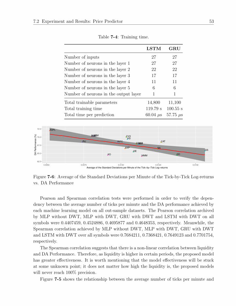
7.2 Experiment and Results: Price Predictor 53
Table 7-4: Training time.
LSTM GRU
Number of inputs 27 27
Number of neurons in the layer 1 27 27
Number of neurons in the layer 2 22 22
Number of neurons in the layer 3 17 17
Number of neurons in the layer 4 11 11
Number of neurons in the layer 5 6 6
Number of neurons in the output layer 1 1
Total trainable parameters 14,800 11,100
Total training time 119.79 s 100.55 s
Total time per prediction 60.04 µs 57.75 µs
AAPL
AXP BA
CATCSCO
CVX
DD
DIS
GE GS
HD
IBMINTCJNJ
JPM
KOMMM
XOM
62.5
65.0
67.5
70.0
72.5
0.0050 0.0075 0.0100 0.0125 0.0150
Average of the Standard Deviations per Minute of the Tick−by−Tick Log−returns
DA
Perf
orm
ance (
%)
Figure 7-6: Average of the Standard Deviations per Minute of the Tick-by-Tick Log-returns
vs. DA Performance
Pearson and Spearman correlation tests were performed in order to verify the depen-
dency between the average number of ticks per minute and the DA performance achieved by
each machine learning model on all out-sample datasets. The Pearson correlation archived
by MLP without DWT, MLP with DWT, GRU with DWT and LSTM with DWT on all
symbols were 0.4407459, 0.4524886, 0.4695877 and 0.4648353, respectively. Meanwhile, the
Spearman correlation achieved by MLP without DWT, MLP with DWT, GRU with DWT
and LSTM with DWT over all symbols were 0.7684211, 0.7368421, 0.7649123 and 0.7701754,
respectively.
The Spearman correlation suggests that there is a non-linear correlation between liquidity
and DA Performance. Therefore, as liquidity is higher in certain periods, the proposed model
has greater effectiveness. It is worth mentioning that the model effectiveness will be stuck
at some unknown point; it does not matter how high the liquidity is, the proposed models
will never reach 100% precision.
Figure 7-5 shows the relationship between the average number of ticks per minute and
54 CHAPTER 7. EXPERIMENTS AND RESULTS
DA performance for each machine learning model. Stocks with higher liquidity (AAPL,
CSCO, and INTC) were excluded for better visualization. As shown in Figure 7-5, the more
traded the stock is, the model predicts it better. Figure 7-5 also draws a fitted Generalized
Additive Model (GAM).
Besides, there is an inverse correlation between the average of the standard deviations per
minute of the tick-by-tick log-returns, and the DA performance achieved by the best model
(GRU with DWT) on all out-sample datasets. Pearson and Spearman correlation tests were
-0.650861 and -0.6573787, respectively. As shown in Figure 7-6, the proposed GRU model
has greater effectiveness as lower as volatility inside a minute is.
7.3 High-Frequency Trading Strategy Simulation
Table 7-5 shows an overview of the experimental setting for testing the proposed high-
frequency trading strategy. Table 7-6 shows the strategy performance during a trading
simulation using the same testing period from the previous chapter (approximately five
months) and the same parameters described in the previous chapter, i.e. it did not take
into account transaction and spread costs. Investment in each stock starts with 1 dollar and
reinvests all the available money in the following operations. Furthermore, Figures 7-8, 7-9
and 7-10 show the three best-performing stocks, whereas Figures 7-11, 7-12 and 7-13 show
the three-worst performing stocks.
Moreover, there are three groups of stocks: the stocks with annualized returns greater
than 100%, the ones with annualized returns between 5% and 100%, and those with less
than 5%. Although DNNs had similar behaviors and remarkable forecasting accuracy, there
are behavior dynamics at the high-frequency scale that are not captured by the aggregated
one-minute series. Additionally, those dynamics are different for each stock.
The best group is composed of CSCO and INTC. Figures 7-8 and 7-9 show both perfor-
mances. The achieved profits had exponential growth behavior. The strategy made 63.5%
and 61.7% good trades, but 36.3% and 38.2% bad trades, respectively. Both average profits
per position are positive. The strategy had a stable and homogeneous behavior for all test-
ing days concerning the number of positions and the amount of buy (long) and sell (short)
positions. Moreover, those two stocks yielded amazing profits.
The worst group is composed of CVX and DD. Figures 7-12 and 7-13 show both per-
formances. Unlike the best group, these stocks had noisy behavior and larger draw-downs.
The strategy made 50.22%, 49.91% and 48.40% good trades, but 49.59% and 48.04% bad
trades, respectively. These stocks were also the only ones that had accumulated losses for a
short time, though they were able to recover and yield earnings.
The third group is composed of the remaining 14 stocks. This group had a similar
behavior compared to the best group. The main differences are that those stocks presented
some draw-downs and yielded high earnings, but not as superior as those of the best group.
All stocks had an annualized volatility raging from 3.54% to 9.01%, with a mean of 5.53%

7.3 High-Frequency Trading Strategy Simulation 55
Table 7-5: Experiment Setting: High-Frequency Trading Strategy
Parameter Value
Number of stocks 18
Time period From April 2017 to September 2017
Duration Approximately 5 months
Transaction costs No
Spread costs No
Initial capital 1 USD
DNN retraining No
Reinvest profits Yes
Table 7-6: Simulation Results.
StockProfit
($)
Annualized
Returns
(%)*
Annualized
Volatility
(%)*
Max
Draw-down
(%)
Earnings
(%)
None
(%)
Losses
(%)
CSCO 4.0297 5528.32 9.01 0.33 63.54 0.16 36.30
INTC 2.8653 2817.78 8.30 0.00 61.69 0.15 38.16
GS 0.2639 79.38 8.86 3.06 50.39 0.70 48.91
GE 0.1601 44.84 5.13 1.08 46.96 8.52 44.52
HD 0.1385 38.21 4.42 1.13 50.78 0.80 48.42
AAPL 0.1189 32.35 8.34 1.91 51.01 0.00 48.99
IBM 0.0985 26.42 4.34 1.20 50.01 1.41 48.58
BA 0.0976 26.16 5.54 1.54 50.10 1.25 48.65
MMM 0.0637 16.65 4.12 1.25 49.27 2.04 48.69
DIS 0.0637 16.65 3.76 0.58 50.05 1.36 48.58
JPM 0.0630 16.48 4.56 1.86 50.26 0.60 49.14
JNJ 0.0555 14.43 3.54 0.89 49.92 1.54 48.54
CAT 0.0490 12.66 5.53 1.75 49.90 1.05 49.04
KO 0.0452 11.66 4.01 2.15 45.88 9.76 44.36
XOM 0.0386 9.91 3.78 1.36 50.22 1.17 48.61
AXP 0.0362 9.27 4.16 2.13 48.65 3.89 47.46
CVX 0.0133 3.36 4.57 2.21 49.91 0.50 49.59
DD 0.0079 1.98 6.53 3.26 48.40 3.57 48.04
*Annualized rates assuming 252 trading days.
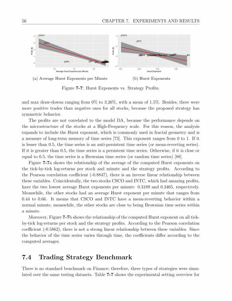
56 CHAPTER 7. EXPERIMENTS AND RESULTS
CSCO
INTC
GSGE HDAAPL IBMBADISMMMJPMJNJCATKO XOMAXPCVXDD0
1
2
3
4
0.4 0.5 0.6
Average Hurst Exponent per Minute
Pro
fit ($
)
(a) Average Hurst Exponents per Minute
CSCO
INTC
GSGEHD IBM BADIS MMMJPM JNJCATKO XOM AXPCVX DD
−2
0
2
4
0.46 0.48 0.50 0.52
Hurst Exponent
Pro
fit ($
)
(b) Hurst Exponents
Figure 7-7: Hurst Exponents vs. Strategy Profits.
and max draw-downs ranging from 0% to 3.26%, with a mean of 1.5%. Besides, there were
more positive trades than negative ones for all stocks, because the proposed strategy has
symmetric behavior.
The profits are not correlated to the model DA, because the performance depends on
the microstructure of the stocks at a High-Frequency scale. For this reason, the analysis
expands to include the Hurst exponent, which is commonly used in fractal geometry and is
a measure of long-term memory of time series [73]. This exponent ranges from 0 to 1. If it
is lesser than 0.5, the time series is an anti-persistent time series (or mean-reverting series).
If it is greater than 0.5, the time series is a persistent time series. Otherwise, if it is close or
equal to 0.5, the time series is a Brownian time series (or random time series) [88].
Figure 7-7a shows the relationship of the average of the computed Hurst exponents on
the tick-by-tick log-returns per stock and minute and the strategy profits. According to
the Pearson correlation coefficient (-0.8847), there is an inverse linear relationship between
these variables. Coincidentally, the two stocks CSCO and INTC, which had amazing profits,
have the two lowest average Hurst exponents per minute: 0.3189 and 0.3465, respectively.
Meanwhile, the other stocks had an average Hurst exponent per minute that ranges from
0.44 to 0.66. It means that CSCO and INTC have a mean-reverting behavior within a
normal minute, meanwhile, the other stocks are close to being Brownian time series within
a minute.
Moreover, Figure 7-7b shows the relationship of the computed Hurst exponent on all tick-
by-tick log-returns per stock and the strategy profits. According to the Pearson correlation
coefficient (-0.5862), there is not a strong linear relationship between these variables. Since
the behavior of the time series varies through time, the coefficients differ according to the
computed averages.
7.4 Trading Strategy Benchmark
There is no standard benchmark on Finance; therefore, three types of strategies were simu-
lated over the same testing datasets. Table 7-7 shows the experimental setting overview for
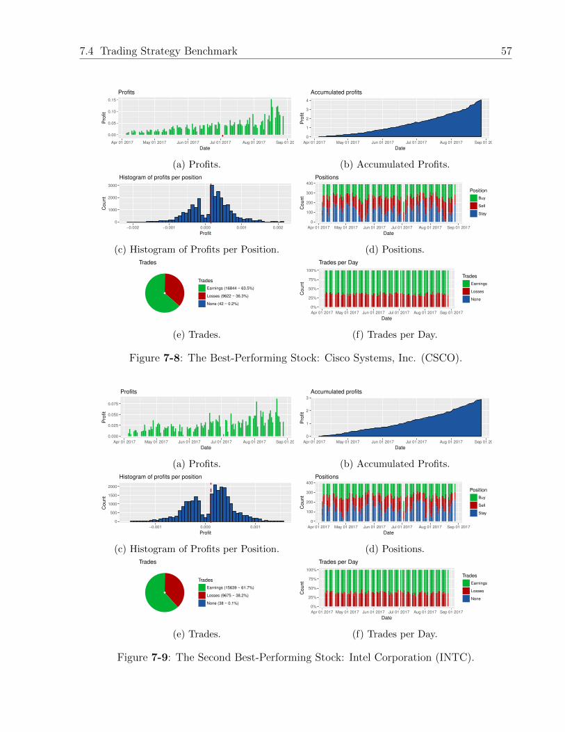
7.4 Trading Strategy Benchmark 57
0.00
0.05
0.10
0.15
Apr 01 2017 May 01 2017 Jun 01 2017 Jul 01 2017 Aug 01 2017 Sep 01 2017
Date
Pro
fit
Profits
(a) Profits.
0
1
2
3
4
Apr 01 2017 May 01 2017 Jun 01 2017 Jul 01 2017 Aug 01 2017 Sep 01 2017
Date
Pro
fit
Accumulated profits
(b) Accumulated Profits.
0
1000
2000
3000
−0.002 −0.001 0.000 0.001 0.002
Profit
Count
Histogram of profits per position
(c) Histogram of Profits per Position.
0
100
200
300
400
Apr 01 2017 May 01 2017 Jun 01 2017 Jul 01 2017 Aug 01 2017 Sep 01 2017
Date
Count
Position
Buy
Sell
Stay
Positions
(d) Positions.
Trades
Earnings (16844 ~ 63.5%)
Losses (9622 ~ 36.3%)
None (42 ~ 0.2%)
Trades
(e) Trades.
0%
25%
50%
75%
100%
Apr 01 2017 May 01 2017 Jun 01 2017 Jul 01 2017 Aug 01 2017 Sep 01 2017
Date
Count
Trades
Earnings
Losses
None
Trades per Day
(f) Trades per Day.
Figure 7-8: The Best-Performing Stock: Cisco Systems, Inc. (CSCO).
0.000
0.025
0.050
0.075
Apr 01 2017 May 01 2017 Jun 01 2017 Jul 01 2017 Aug 01 2017 Sep 01 2017
Date
Pro
fit
Profits
(a) Profits.
0
1
2
3
Apr 01 2017 May 01 2017 Jun 01 2017 Jul 01 2017 Aug 01 2017 Sep 01 2017
Date
Pro
fit
Accumulated profits
(b) Accumulated Profits.
0
500
1000
1500
2000
−0.001 0.000 0.001
Profit
Count
Histogram of profits per position
(c) Histogram of Profits per Position.
0
100
200
300
400
Apr 01 2017 May 01 2017 Jun 01 2017 Jul 01 2017 Aug 01 2017 Sep 01 2017
Date
Count
Position
Buy
Sell
Stay
Positions
(d) Positions.
Trades
Earnings (15639 ~ 61.7%)
Losses (9675 ~ 38.2%)
None (38 ~ 0.1%)
Trades
(e) Trades.
0%
25%
50%
75%
100%
Apr 01 2017 May 01 2017 Jun 01 2017 Jul 01 2017 Aug 01 2017 Sep 01 2017
Date
Count
Trades
Earnings
Losses
None
Trades per Day
(f) Trades per Day.
Figure 7-9: The Second Best-Performing Stock: Intel Corporation (INTC).

58 CHAPTER 7. EXPERIMENTS AND RESULTS
−0.01
0.00
0.01
0.02
Apr 01 2017 May 01 2017 Jun 01 2017 Jul 01 2017 Aug 01 2017 Sep 01 2017
Date
Pro
fit
Profits
(a) Profits.
0.0
0.1
0.2
Apr 01 2017 May 01 2017 Jun 01 2017 Jul 01 2017 Aug 01 2017 Sep 01 2017
Date
Pro
fit
Accumulated profits
(b) Accumulated Profits.
0
500
1000
1500
2000
−1e−03 −5e−04 0e+00 5e−04 1e−03
Profit
Count
Histogram of profits per position
(c) Histogram of Profits per Position.
0
100
200
300
400
Apr 01 2017 May 01 2017 Jun 01 2017 Jul 01 2017 Aug 01 2017 Sep 01 2017
Date
Count
Position
Buy
Sell
Stay
Positions
(d) Positions.
Trades
Earnings (14586 ~ 50.4%)
Losses (14159 ~ 48.9%)
None (202 ~ 0.7%)
Trades
(e) Trades.
0%
25%
50%
75%
100%
Apr 01 2017 May 01 2017 Jun 01 2017 Jul 01 2017 Aug 01 2017 Sep 01 2017
Date
Count
Trades
Earnings
Losses
None
Trades per Day
(f) Trades per Day.
Figure 7-10: The Third Best-Performing Stock: Goldman Sachs Group, Inc. (GS).
−0.005
0.000
0.005
0.010
Apr 01 2017 May 01 2017 Jun 01 2017 Jul 01 2017 Aug 01 2017 Sep 01 2017
Date
Pro
fit
Profits
(a) Profits.
0.00
0.01
0.02
0.03
0.04
Apr 01 2017 May 01 2017 Jun 01 2017 Jul 01 2017 Aug 01 2017 Sep 01 2017
Date
Pro
fit
Accumulated profits
(b) Accumulated Profits.
0
1000
2000
3000
4000
5000
−6e−04 −3e−04 0e+00 3e−04 6e−04
Profit
Count
Histogram of profits per position
(c) Histogram of Profits per Position.
0
100
200
300
400
Apr 01 2017 May 01 2017 Jun 01 2017 Jul 01 2017 Aug 01 2017 Sep 01 2017
Date
Count
Position
Buy
Sell
Stay
Positions
(d) Positions.
Trades
Earnings (10505 ~ 48.7%)
Losses (10247 ~ 47.5%)
None (839 ~ 3.9%)
Trades
(e) Trades.
0%
25%
50%
75%
100%
Apr 01 2017 May 01 2017 Jun 01 2017 Jul 01 2017 Aug 01 2017 Sep 01 2017
Date
Count
Trades
Earnings
Losses
None
Trades per Day
(f) Trades per Day.
Figure 7-11: The Third Worst-Performing Stock: American Express Company (AXP).
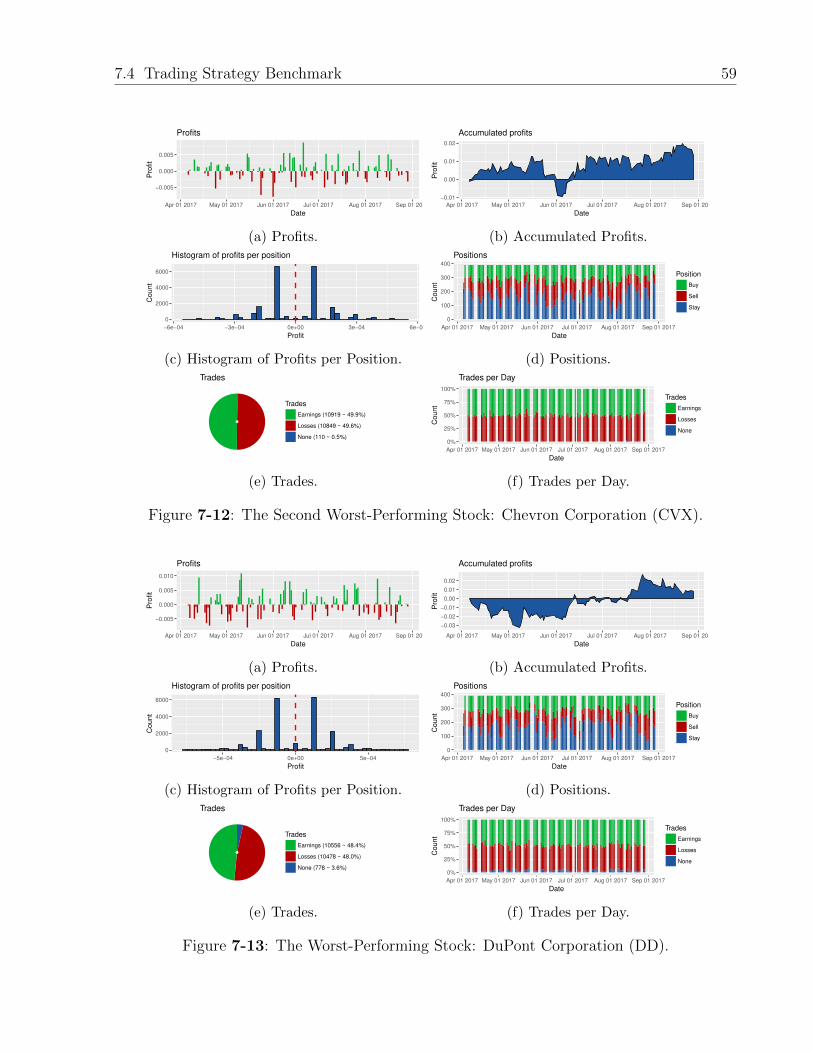
7.4 Trading Strategy Benchmark 59
−0.005
0.000
0.005
Apr 01 2017 May 01 2017 Jun 01 2017 Jul 01 2017 Aug 01 2017 Sep 01 2017
Date
Pro
fit
Profits
(a) Profits.
−0.01
0.00
0.01
0.02
Apr 01 2017 May 01 2017 Jun 01 2017 Jul 01 2017 Aug 01 2017 Sep 01 2017
Date
Pro
fit
Accumulated profits
(b) Accumulated Profits.
0
2000
4000
6000
−6e−04 −3e−04 0e+00 3e−04 6e−04
Profit
Count
Histogram of profits per position
(c) Histogram of Profits per Position.
0
100
200
300
400
Apr 01 2017 May 01 2017 Jun 01 2017 Jul 01 2017 Aug 01 2017 Sep 01 2017
Date
Count
Position
Buy
Sell
Stay
Positions
(d) Positions.
Trades
Earnings (10919 ~ 49.9%)
Losses (10849 ~ 49.6%)
None (110 ~ 0.5%)
Trades
(e) Trades.
0%
25%
50%
75%
100%
Apr 01 2017 May 01 2017 Jun 01 2017 Jul 01 2017 Aug 01 2017 Sep 01 2017
Date
Count
Trades
Earnings
Losses
None
Trades per Day
(f) Trades per Day.
Figure 7-12: The Second Worst-Performing Stock: Chevron Corporation (CVX).
−0.005
0.000
0.005
0.010
Apr 01 2017 May 01 2017 Jun 01 2017 Jul 01 2017 Aug 01 2017 Sep 01 2017
Date
Pro
fit
Profits
(a) Profits.
−0.03
−0.02
−0.01
0.00
0.01
0.02
Apr 01 2017 May 01 2017 Jun 01 2017 Jul 01 2017 Aug 01 2017 Sep 01 2017
Date
Pro
fit
Accumulated profits
(b) Accumulated Profits.
0
2000
4000
6000
−5e−04 0e+00 5e−04
Profit
Count
Histogram of profits per position
(c) Histogram of Profits per Position.
0
100
200
300
400
Apr 01 2017 May 01 2017 Jun 01 2017 Jul 01 2017 Aug 01 2017 Sep 01 2017
Date
Count
Position
Buy
Sell
Stay
Positions
(d) Positions.
Trades
Earnings (10556 ~ 48.4%)
Losses (10478 ~ 48.0%)
None (778 ~ 3.6%)
Trades
(e) Trades.
0%
25%
50%
75%
100%
Apr 01 2017 May 01 2017 Jun 01 2017 Jul 01 2017 Aug 01 2017 Sep 01 2017
Date
Count
Trades
Earnings
Losses
None
Trades per Day
(f) Trades per Day.
Figure 7-13: The Worst-Performing Stock: DuPont Corporation (DD).

60 CHAPTER 7. EXPERIMENTS AND RESULTS
Table 7-7: Experiment Setting: Trading Strategy Benchmark
StrategyNumber of
stocksTime period
Transaction
costs
Spread
costs
Initial
capital
Proposed Strategy
18
From April 2017
to September 2017
(Approximately
5 months)
No No 1 USD
Buy & Hold
RSI Strategy (4 mins.)
RSI Strategy (9 mins.)
RSI Strategy (14 mins.)
RSI Strategy (19 mins.)
RSI Strategy (24 mins.)
RSI Strategy (29 mins.)
Random Trading
comparing the proposed high-frequency trading strategy against the three types of strate-
gies. Table 7-8 shows the simulation results. Moreover, Figure 7-14 shows the accumulated
profit per each strategy. The chosen strategies were:
Buy & Hold Strategy (BHS)
A BHS is a passive investment strategy in which a trader buys a stock (opens a long position),
and holds it in his portfolio for a long time, while, he expects the stock value increases over-
time. The BHS lost money with six stocks: INTC, GE, IBM, XOM, AXP, CVX. In contrast,
the proposed strategy earned money with all stocks. If a portfolio had been created with
18 stocks and $1 for each stock, the BHS would have to earn $2.9897, and the proposed
strategy would have to earn $8.2353 (approximately 2.7 times more).
RSI Trading Strategy
For each minute, the Relative Strength Index (RSI) was computed using n one-minute peri-
ods. If the asset is overbought, the strategy sells the asset and then buys it when the minute
ends. If the asset is oversold, the strategy buys the asset and then sells it when the minute
ends. Otherwise, the strategy does not do anything until the next minute. The chosen n
were 4, 9, 14, 19, 24 and 29, and the chosen oversold and overbought thresholds were 20 and
80, respectively.
All the RSI strategies yielded positive returns. The profit was lesser to the yielded by
the proposed strategy and the Buy & Hold Strategy. The best performing configuration was
n = 4, and the worst was n = 29.

7.4 Trading Strategy Benchmark 61
Table 7-8: Strategy Benchmark.
StockProposed
Strategy
Buy &
Hold
RSI Strategy Random
Trading4 mins. 9 mins. 14 mins. 19 mins. 24 mins. 29 mins.
CSCO 4.0297 0.1317 0.2930 -0.0427 0.0003 0.0387 0.0288 0.0278 -0.0152
INTC 2.8653 -0.0564 0.4479 0.1298 0.0231 0.0242 0.0231 0.0122 0.0123
GS 0.2639 0.1262 0.2435 0.0320 -0.0032 -0.0007 -0.0100 -0.0225 0.0031
GE 0.1601 -0.0372 0.2714 0.0866 0.0447 0.0259 0.0185 0.0211 0.0270
HD 0.1385 0.4229 0.0456 0.0262 -0.0007 -0.0091 -0.0180 -0.0172 -0.0034
AAPL 0.1189 0.4496 0.0875 0.0383 0.0402 0.0207 0.0142 0.0039 -0.0052
IBM 0.0985 -0.1132 0.0640 0.0077 -0.0032 0.0001 0.0028 0.0058 0.0059
BA 0.0976 0.8369 -0.0136 -0.0362 -0.0369 -0.0429 -0.0285 -0.0263 0.0148
MMM 0.0637 0.2366 0.0607 -0.0138 -0.0272 -0.0255 -0.0260 -0.0239 -0.0002
DIS 0.0637 0.0805 0.0372 0.0255 0.0148 0.0247 0.0193 0.0236 -0.0021
JPM 0.0630 0.4542 0.2267 0.0759 0.0315 0.0123 0.0105 0.0168 -0.0167
JNJ 0.0555 0.2560 0.0125 0.0566 0.0186 0.0121 0.0119 0.0044 0.0071
CAT 0.0490 0.2638 0.0704 0.0135 0.0146 0.0088 0.0009 -0.0055 0.0226
KO 0.0452 0.0750 0.2190 0.0549 0.0167 0.0145 0.0112 -0.0016 0.0071
XOM 0.0386 -0.1716 0.1510 0.0065 -0.0057 -0.0083 -0.0053 -0.0022 -0.0098
AXP 0.0362 -0.0860 0.0933 0.0321 0.0277 0.0226 0.0196 0.0120 -0.0033
CVX 0.0133 -0.0349 0.0335 -0.0004 0.0024 -0.0047 -0.0101 -0.0056 0.0022
DD 0.0079 0.1140 0.1432 0.0726 0.0414 0.0275 0.0323 0.0242 0.0143
Total 8.2086 2.9481 2.4868 0.5651 0.1991 0.1409 0.0952 0.0470 0.0605
One-minute Random Trading Strategy
For each minute, a long or short operation is opened and then closed when the minute ends.
The decision is taken randomly. Depending on the run, the strategy can obtain earnings or
losses. Therefore, 100 simulations were performed and the average profit was reported. This
average profit is very close to 0.
Besides, the proposed strategy adds some advantages: First, the predictor of the strategy
can be retrained in less than two minutes in standard hardware at any time (If it is required to
reduce training times, hardware with better capabilities can be used). Second, the predictions
can be performed in real-time. Third, the strategy is simple and can be implemented in any
trading platform. And finally, the strategy has a symmetric behavior at opening and closings
signals.
The proposed strategy has stable performance, though it is necessary to extend the
analyzes to consider transaction costs, spreads, and liquidity in high-frequency. At the time
of the development of this work, we did not have access to the best bid-ask series or limit
order books. For this reason, we can not perform a perfect simulation that includes all
those hidden costs such as the spread. Hence, we will estimate the average spread, and
then, will make a small analysis of the strategy’s performance when a constant spread cost
is introduced. It is important to note that the spread is variable over time, and in order to
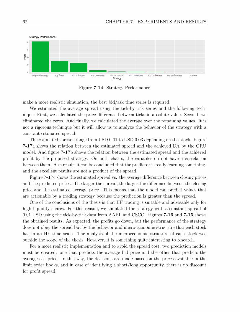
62 CHAPTER 7. EXPERIMENTS AND RESULTS
0
2
4
6
8
Proposed Strategy Buy & Hold RSI (4 Minutes) RSI (9 Minutes) RSI (14 Minutes) RSI (19 Minutes) RSI (24 Minutes) RSI (29 Minutes) Random
Strategy
Pro
fit
Strategy Performance
Figure 7-14: Strategy Performance
make a more realistic simulation, the best bid/ask time series is required.
We estimated the average spread using the tick-by-tick series and the following tech-
nique: First, we calculated the price difference between ticks in absolute value. Second, we
eliminated the zeros. And finally, we calculated the average over the remaining values. It is
not a rigorous technique but it will allow us to analyze the behavior of the strategy with a
constant estimated spread.
The estimated spreads range from USD 0.01 to USD 0.03 depending on the stock. Figure
7-17a shows the relation between the estimated spread and the achieved DA by the GRU
model. And figure 7-17b shows the relation between the estimated spread and the achieved
profit by the proposed strategy. On both charts, the variables do not have a correlation
between them. As a result, it can be concluded that the predictor is really learning something,
and the excellent results are not a product of the spread.
Figure 7-17c shows the estimated spread vs. the average difference between closing prices
and the predicted prices. The larger the spread, the larger the difference between the closing
price and the estimated average price. This means that the model can predict values that
are actionable by a trading strategy because the prediction is greater than the spread.
One of the conclusions of the thesis is that HF trading is suitable and advisable only for
high liquidity shares. For this reason, we simulated the strategy with a constant spread of
0.01 USD using the tick-by-tick data from AAPL and CSCO. Figures 7-16 and 7-15 shows
the obtained results. As expected, the profits go down, but the performance of the strategy
does not obey the spread but by the behavior and micro-economic structure that each stock
has in an HF time scale. The analysis of the microeconomic structure of each stock was
outside the scope of the thesis. However, it is something quite interesting to research.
For a more realistic implementation and to avoid the spread cost, two prediction models
must be created: one that predicts the average bid price and the other that predicts the
average ask price. In this way, the decisions are made based on the prices available in the
limit order books, and in case of identifying a short/long opportunity, there is no discount
for profit spread.

7.4 Trading Strategy Benchmark 63
−0.008
−0.004
0.000
0.004
0.008
0.012
Apr 01 2017 May 01 2017 Jun 01 2017 Jul 01 2017 Aug 01 2017 Sep 01 2017
Date
Pro
fit
Profits
(a) Profits.
0.00
0.05
0.10
0.15
0.20
Apr 01 2017 May 01 2017 Jun 01 2017 Jul 01 2017 Aug 01 2017 Sep 01 2017
Date
Pro
fit
Accumulated profits
(b) Accumulated Profits.
0
100
200
−0.002 −0.001 0.000 0.001 0.002
Profit
Count
Histogram of profits per position
(c) Histogram of Profits per Position.
0
100
200
300
400
Apr 01 2017 May 01 2017 Jun 01 2017 Jul 01 2017 Aug 01 2017 Sep 01 2017
Date
Count
Position
Buy
Sell
Stay
Positions
(d) Positions.
Trades
Earnings (681 ~ 84.1%)
Losses (129 ~ 15.9%)
None (0 ~ 0.0%)
Trades
(e) Trades.
0%
25%
50%
75%
100%
Apr 01 2017 May 01 2017 Jun 01 2017 Jul 01 2017 Aug 01 2017 Sep 01 2017
Date
Count
Trades
Earnings
Losses
None
Trades per Day
(f) Trades per Day.
Figure 7-15: Cisco Inc. (CSCO): Estimated spread USD 0.01
0.000
0.005
0.010
0.015
0.020
0.025
Apr 01 2017 May 01 2017 Jun 01 2017 Jul 01 2017 Aug 01 2017 Sep 01 2017
Date
Pro
fit
Profits
(a) Profits.
0.00
0.05
0.10
0.15
Apr 01 2017 May 01 2017 Jun 01 2017 Jul 01 2017 Aug 01 2017 Sep 01 2017
Date
Pro
fit
Accumulated profits
(b) Accumulated Profits.
0
300
600
900
1200
−1e−03 −5e−04 0e+00 5e−04 1e−03
Profit
Count
Histogram of profits per position
(c) Histogram of Profits per Position.
0
100
200
300
400
Apr 01 2017 May 01 2017 Jun 01 2017 Jul 01 2017 Aug 01 2017 Sep 01 2017
Date
Count
Position
Buy
Sell
Stay
Positions
(d) Positions.
Trades
Earnings (3956 ~ 63.1%)
Losses (2309 ~ 36.9%)
None (0 ~ 0.0%)
Trades
(e) Trades.
0%
25%
50%
75%
100%
Apr 01 2017 May 01 2017 Jun 01 2017 Jul 01 2017 Aug 01 2017 Sep 01 2017
Date
Count
Trades
Earnings
Losses
None
Trades per Day
(f) Trades per Day.
Figure 7-16: Apple Inc. (AAPL): Estimated spread USD 0.01

64 CHAPTER 7. EXPERIMENTS AND RESULTS
^[
^\
^]
^^
^_
^`
^a
_X
_Y
_Z
_[
X XáXX] XáXY XáXY] XáXZ XáXZ] XáX[ XáX[]
®
(a) Estimated spread vs. Directional Accuracy
X
Xá]
Y
Yá]
Z
Zá]
[
[á]
\
\á]
X XáXX] XáXY XáXY] XáXZ XáXZ] XáX[ XáX[]
F
(b) Estimated spread vs. Profit
³Xá\Y]^
X
XáY
XáZ
Xá[
Xá\
Xá]
Xá^
X XáXX] XáXY XáXY] XáXZ XáXZ] XáX[ XáX[]
F
(c) Spread Analysis: Diff
Figure 7-17: Spread Analysis

Chapter 8
Conclusions and Recommendations
The main motivation of this thesis was to help build a bridge between the financial industry
and academic research, providing experience and new approaches to improve understanding
of the markets. Moreover, this work seeks to be a public base work for academic and
industrial research in financial machine learning, which is a new multidisciplinary world
that is being born and will revolutionize the financial industry [28]. This new discipline
needs non-standard procedures, techniques, and approaches (such as those presented in this
document) that differs from the standard machine learning world. Therefore, works like this
are needed to continue with this revolution.
The main contribution of this work is the proposed innovative approach for predicting
FTS. It includes the combination of:
• The advanced learning capabilities of the Deep RNN (LSTM and GRU).
• The representational power in frequency and time domains of the DWT.
• And the idea of modeling time series through average prices.
Many works have studied the prediction of FTS and suggested to explore more learning
techniques and complicated features [117, 71, 39, 12]. Being motivated by the previous
reasons, this work explored DL models (more specifically, RNN like LSTM and GRU) and
the combination of multiple features (the time, one-minute standard deviations, one-minute
trend indicators, one-minute log-returns, Fourier coefficients, wavelet coefficients, among
others).
Moreover, this work proposes a straightforward high-frequency trading strategy that uses
the proposed DNN predictor. It supports the idea behind the pseudo-log-returns: Predicting
an average price is easier than predicting a closing price, that is, the product of a random
and noisy process. This strategy presented highly competitive results (see Chapter 7).
Besides, an average price can be better exploited in a trading strategy, than a closing
price. The reason is that average prices predictions have less uncertainty than those of

66 CHAPTER 8. CONCLUSIONS AND RECOMMENDATIONS
closing prices. Hence, making decisions with less uncertainty leads to trades with less risk
and greater possibilities of carrying out successful trades. Below the main conclusions and
recommendations will be presented:
Discrete Wavelet Transform
• The main advantage of using DWT is that the resulting time series is represented in
the frequency domain with temporal resolution; hence, the signal has properties from
both time and frequency domains.
• The Haar wavelet has a technical disadvantage: It has discontinuities and hence it is
not a differentiable function. However, its discontinuities are an advantage for FTS
analysis because they perfectly fit to handle signals with sudden transitions and jumps.
• Without the features of using the DWT, the DNN had not been able to learn the
complex and intricate patterns of FTS. Therefore, DWT has proved to be an important
tool for time series analysis and prediction.
• The proposed preprocessing method based on the DWT works with any signal of any
length greater to 8. This property is useful for homogenizing data in fixed shape size
because any machine learning technique can use this resulting data.
• Besides, this preprocessing method allows the proposed predictor to exploit and take
advantage of the available information at an HF scale.
• The DWT is easy to program within any trading strategy since there are many robust
packages and libraries in most popular programming languages.
Deep Learning
• The use of an RNN allowed achieving better results than a simple MLP because RNN
has an internal memory that allows modeling temporal dynamics.
• The DL arena has a lot of robust techniques that can face the difficult task of pre-
dicting FTS and modeling market behavior because they can learn a deep hierarchical
representation of data, in which the input is transformed from low-level to high-level
representations.
• The proposed predictor can be trained in less than two minutes in standard hardware
at any time (If it is required to reduce training times, hardware with better capabilities
can be used). This property is useful for online retraining if required.

67
• GPUs increased the speed of training DL models because they are suitable for massive
linear algebra operations involved in training algorithms.
• The use of adaptive optimizers guaranteed a fast convergence in the ANN parameters.
Feature Engineering
• It is important to note that feature engineering is an essential step on any machine
learning project. Currently, the end-to-end approach, in which the models are based on
raw data, and feature engineering is not required, is the most common DL approach in
many disciplines. However, this approach is not recommended for finance applications
(at least not with the current advances in hardware and machine learning techniques),
due to the excessive complexity and properties of FTS.
• Due to restrictions when the strategy is operating at High-Frequency scale, the pre-
diction model inputs must be able to be calculated fast.
Pseudo-log-returns
• Pseudo-log-returns, which are a non-standard data transformation, offer more quality
information on the status of an asset price. Given the fact that averages are more
stable than noisy tick-by-tick prices, they are less affected by outliers and noise than
log-returns.
• Another approach would be to use the median that is more stable than the average.
However, given the time and speed constraints at High-Frequency scale, it is more
recommended to use the average prices, because the calculation of the median implies
sorting the tick-by-tick prices and this process is performed in O(n log n). Meanwhile,
the calculation of the average can be performed in O(n).
• Besides, this work differs from others in the use of the concept of pseudo-log-returns. It
allowed the proposed prediction model to achieve better performance since the average
prices are less exposed to noise.
• Predicting average prices is an easier task than predicting closing prices. Depending on
the financial asset, its liquidity and the amount of trades within a minute, the average
becomes an estimator of greater confidence and supplies more valuable information
about the market status. Therefore, it is easier for a DNN or any machine learning
model to predict average prices than closing prices.
• Pseudo-log-returns are easy to implement in any programming language; therefore,
they can be integrated into a trading strategy in any algorithmic trading platform.
68 CHAPTER 8. CONCLUSIONS AND RECOMMENDATIONS
Liquid stocks
• In this study, the proposed DNN achieved 72% of directional accuracy, predicting the
Apple Inc. stock (AAPL), which has the highest average number of trades per minute
within the dataset. Found evidence suggests that the performance of the prediction
model has a non-linear correlation with the number of trades per minute. As the
amount of ticks increases, the prediction also improves because the averages are more
stable and reliable.
High-Frequency Trading Strategy
• An average price estimation can be better exploited in a trading strategy than a closing
price estimation.
• There is evidence that not operating in all minutes can be crucial for the excellent
performance of the strategy. The reason is that opening and closing positions in
minutes of high volatility or low liquids can be a bad idea for HF strategies.
• Given the fact that there is no guarantee of knowing whether the next minute will
be enough liquid to operate, in this work, a policy was suggested: do not trade if
the traded volume of the previous minute does not exceed a threshold. This policy is
straightforward but effective.
• Found evidence suggests that there is an inverse linear relationship of the average of the
computed Hurst exponents on the tick-by-tick log-returns per minute and the strategy
profits.

Chapter 9
Opportunities for Future Research
This work presented highly competitive results. There are many possible opportunities for
future research that are derived from this work and seek to improve it:
Discrete Wavelet Transform
• The Haar wavelet discontinuities perfectly fit to handle signals with sudden transitions
like FTS. However, a possible research opportunity would be to explore the performance
of other wavelets (Daubechies, Coiflets, Symlets, Discrete Meyer, Biorthogonal, among
others), as well as other discrete transforms like Discrete Chebyshev transform and
Discrete cosine transform.
• It might also be interesting to include higher resolution levels as inputs to the DNN,
in order to analyze if adding more wavelet and scaling coefficients, the prediction
performance can improve.
Deep Learning
• Another possible opportunity for research is to explore other DL architectures like
Deep Convolutional Neural Networks or Deep Belief Networks, or even other Machine
Learning techniques that allow incorporating expert knowledge, such as Hidden Markov
Model (HMM) and Dynamic Bayesian Networks.
Feature Engineering
• This research could also be extended to studying available data on Limit Order Books
(LOB), volume time series, external news, earnings reports, technical indicators, among
others. It could allow extracting more knowledge and identify more complex patterns

70 CHAPTER 9. OPPORTUNITIES FOR FUTURE RESEARCH
from the market at an HF scale. With a better understanding of market status, the
model will be able to make better decisions and yield higher and more stable profits.
Trading Strategy
• The presented strategy is simple and yielded good performance. However, it must be
refined for implementing it in a real environment. It is necessary to extend the analysis
including transaction costs and distribution, as can this can be crucial to the strategy
viability.
• For deciding if a minute is suitable for trading, the proposed policy is straightfor-
ward, but effective, in order to handle the volatility or low liquids changing conditions.
However, it can be refined by implementing reinforcement learning to determine if the
next minute should be operated at the high-frequency scale. In summary, including
reinforcement learning is an excellent possible research opportunity.
• It will be interesting to extend the analysis in order to consider what is the useful
life of a machine learning model, and what would be the rate to retrain for a real
implementation.
• Finally, a clustering algorithm or another technique can be used to choose a group of
stocks and build a portfolio. So, the proposed method of this dissertation can be used
to manage positions for each selected stock.
Bibliography
[1] Abu-Mostafa, Yaser S. ; Atiya, Amir F.: Introduction to financial forecasting. In:
Applied Intelligence 6 (1996), Nr. 3, S. 205–213
[2] ACM, the Association for Computing M.: Fathers of the Deep Learning Revolu-
tion Receive ACM A.M. Turing Award. https://www.acm.org/media-center/2019/
march/turing-award-2018. Version: 2019
[3] Aiba, Yukihiro ; Hatano, Naomichi ; Takayasu, Hideki ; Marumo, Kouhei ;
Shimizu, Tokiko: Triangular arbitrage as an interaction among foreign exchange rates.
In: Physica A: Statistical Mechanics and its Applications 310 (2002), Nr. 3-4, S. 467–
479. http://dx.doi.org/10.1016/S0378-4371(02)00799-9. – DOI 10.1016/S0378–
4371(02)00799–9. – ISBN 0378–4371
[4] Aizenberg, Igor N. ; Aizenberg, Naum N. ; Vandewalle, Joos: Multi-Valued
and Universal Binary Neurons. Springer US, 2000. http://dx.doi.org/10.1007/
978-1-4757-3115-6. http://dx.doi.org/10.1007/978-1-4757-3115-6
[5] Aldridge, I: High-Frequency Trading: A Practical Guide to Algorithmic Strategies
and Trading Systems. Wiley, 2009 (Wiley Trading). https://books.google.com.co/
books?id=fEXKZAAVu4oC. – ISBN 9780470579770
[6] Amjady, N ; Hemmati, M: Day-ahead price forecasting of electricity markets by a
hybrid intelligent system. In: European Transactions on Electrical Power 19 (2009),
Nr. 1, 89–102. http://dx.doi.org/10.1002/etep.242. – DOI 10.1002/etep.242. –
ISSN 1430144X (ISSN)
[7] Arevalo, Andres ; Nino, Jaime ; Hernandez, German ; Sandoval, Javier: High-
frequency trading strategy based on deep neural networks. In: Lecture Notes in Com-
puter Science (including subseries Lecture Notes in Artificial Intelligence and Lecture
Notes in Bioinformatics) Bd. 9773, Springer International Publishing, 2016. – ISBN
978–3–319–42296–1, 424–436
[8] Arevalo Murillo, Andres R.: Short-Term Forecasting of Financial Time Series
with Deep Neural Networks. In: bdigital.unal.edu.co (2016). http://www.bdigital.
unal.edu.co/54538/

72 BIBLIOGRAPHY
[9] Armano, G ; Marchesi, M ; Murru, A: A hybrid genetic-neural architecture for
stock indexes forecasting. In: Information Sciences 170 (2005), Nr. 1, 3–33. http://
dx.doi.org/10.1016/j.ins.2003.03.023. – DOI 10.1016/j.ins.2003.03.023. – ISSN
00200255 (ISSN)
[10] Arnold, L ; Rebecchi, S ; Chevallier, S ; Paugam-Moisy, H: An Introduction
to Deep Learning. In: ESANN (2011). https://www.elen.ucl.ac.be/Proceedings/
esann/esannpdf/es2011-4.pdf
[11] Bachelier, L: Theorie de la speculation. In: Annales scientifiques de l’Ecole Normale
Superieure Bd. 17 Elsevier, 1900, S. 21–86
[12] Bao, Wei ; Yue, Jun ; Rao, Yulei: A deep learning framework for financial time
series using stacked autoencoders and long-short term memory. In: PLOS ONE 12
(2017), Nr. 7, 1–24. http://dx.doi.org/10.1371/journal.pone.0180944. – DOI
10.1371/journal.pone.0180944
[13] Bengio, Yoshua: Learning Deep Architectures for AI. In: Foundations and Trends?
in Machine Learning 2 (2009), 1, Nr. 1, 1–127. http://dx.doi.org/10.1561/
2200000006. – DOI 10.1561/2200000006. – ISSN 1935–8237
[14] Bouveret, Antoine ; Guillaumie, Cyrille ; Roqueiro, Carlos A. ; Winkler,
Christian ; Nauhaus, Steffen: High-frequency trading activity in EU equity markets.
In: European Securities and Markets Authority, Economic Report 2014 (2014), Nr. 1,
S. 1–31
[15] Box, George E P. ; Jenkins, Gwilym M. ; MacGregor, John F.: Some recent
advances in forecasting and control. In: Applied Statistics (1974), S. 158–179
[16] Buscema, M ; Sacco, P L.: Feedforward networks in financial predictions:
The future that modifies the present. In: Expert Systems 17 (2000), Nr. 3,
149–170. https://www.scopus.com/inward/record.uri?eid=2-s2.0-0034223894&
partnerID=40&md5=77cf1a1159378975b6471d9cc7b3884d. – ISSN 02664720 (ISSN)
[17] Carter, Bruce ; Mancini, Ron: Op Amps for everyone. Newnes, 2017
[18] Chan, E: Quantitative Trading: How to Build Your Own Algorithmic Trading Busi-
ness. Wiley, 2009 (Wiley Trading). https://books.google.com.co/books?id=
NZlV0M5Ije4C. – ISBN 9780470466261
[19] Chang, P.-C. ; Fan, C.-Y. ; Liu, C.-H.: Integrating a piecewise linear representation
method and a neural network model for stock trading points prediction. In: IEEE
Transactions on Systems, Man and Cybernetics Part C: Applications and Reviews 39
(2009), Nr. 1, 80–92. http://dx.doi.org/10.1109/TSMCC.2008.2007255. – DOI
10.1109/TSMCC.2008.2007255. – ISSN 10946977 (ISSN)

BIBLIOGRAPHY 73
[20] Chao, Jing ; Shen, Furao ; Zhao, Jinxi: Forecasting exchange rate with deep belief
networks. In: The 2011 International Joint Conference on Neural Networks, IEEE, 7
2011. – ISBN 978–1–4244–9635–8, 1259–1266
[21] Chen, A.-S. ; Leung, M T.: Regression neural network for error correction in foreign
exchange forecasting and trading. In: Computers and Operations Research 31 (2004),
Nr. 7, 1049–1068. http://dx.doi.org/10.1016/S0305-0548(03)00064-9. – DOI
10.1016/S0305–0548(03)00064–9. – ISSN 03050548 (ISSN)
[22] Chen, Kai ; Zhou, Yi ; Dai, Fangyan: A LSTM-based method for stock returns
prediction: A case study of China stock market. In: Proceedings - 2015 IEEE In-
ternational Conference on Big Data, IEEE Big Data 2015, IEEE, 10 2015. – ISBN
9781479999255, 2823–2824
[23] Chlistalla, Michael: High Frequency Trading, better than its reputation? In:
Deutsche Bank Research 8 (2011), Nr. 3, 217–224. http://dx.doi.org/10.1080/
14697680701381228. – DOI 10.1080/14697680701381228. – ISBN 9781782720096
[24] Cho, Kyunghyun ; Merrienboer, Bart van ; Gulcehre, Caglar ; Bahdanau,
Dzmitry ; Bougares, Fethi ; Schwenk, Holger ; Bengio, Yoshua: Learning Phrase
Representations using RNN Encoder-Decoder for Statistical Machine Translation. In:
Proceedings of the 2014 Conference on Empirical Methods in Natural Language Pro-
cessing (EMNLP) (2014), 6, 1724–1734. http://dx.doi.org/10.3115/v1/D14-1179.
– DOI 10.3115/v1/D14–1179. – ISBN 9781937284961
[25] De Gooijer, Jan G. ; Hyndman, Rob J.: 25 years of time series forecasting. In:
International Journal of Forecasting 22 (2006), 1, Nr. 3, 443–473. http://dx.doi.
org/10.1016/j.ijforecast.2006.01.001. – DOI 10.1016/j.ijforecast.2006.01.001. –
ISSN 01692070
[26] De Gooijer, Jan G. ; Kumar, Kuldeep: Some recent developments in non-linear
time series modelling, testing, and forecasting. In: International Journal of Forecasting
8 (1992), 10, Nr. 2, 135–156. http://dx.doi.org/10.1016/0169-2070(92)90115-P.
– DOI 10.1016/0169–2070(92)90115–P. – ISSN 01692070
[27] De Oliveira, F A. ; Nobre, C N. ; Zarate, L E.: Applying Artificial Neural
Networks to prediction of stock price and improvement of the directional prediction
index - Case study of PETR4, Petrobras, Brazil. In: Expert Systems with Applications
40 (2013), Nr. 18, 7596–7606. http://dx.doi.org/10.1016/j.eswa.2013.06.071. –
DOI 10.1016/j.eswa.2013.06.071. – ISSN 09574174 (ISSN)
[28] De Prado, Marcos L.: Advances in financial machine learning. John Wiley & Sons,
2018

74 BIBLIOGRAPHY
[29] Debao, Chen: Degree of approximation by superpositions of a sigmoidal function.
In: Approximation Theory and its Applications 9 (1993), Nr. 3, S. 17–28. http://dx.
doi.org/10.1007/BF02836480. – DOI 10.1007/BF02836480. – ISBN 0780300564
[30] Dechter, Rina: Learning While Searching in Constraint-satisfaction-problems. In:
Proceedings of the Fifth AAAI National Conference on Artificial Intelligence, AAAI
Press, 1986 (AAAI’86), 178–183
[31] Di Persio, L ; Honchar, O: Artificial neural networks architectures
for stock price prediction: Comparisons and applications. In: Interna-
tional Journal of Circuits, Systems and Signal Processing 10 (2016), 403–
413. https://www.scopus.com/inward/record.uri?eid=2-s2.0-84998705847&
partnerID=40&md5=f3fa06042299716f81a58ef587947ec2. – ISSN 19984464 (ISSN)
[32] Dijk, Mathijs van: The Social Value of Finance. 2014
[33] Ding, X ; Zhang, Y ; Liu, T ; Duan, J: Deep learning for event-driven stock predic-
tion. In: Proceedings of the Twenty-Fourth International Joint Conference on Artificial
Intelligence (ICJAI) (2015). http://ijcai.org/papers15/Papers/IJCAI15-329.
[34] Dunis, Christian L. ; Jalilov, Jamshidbek: Neural Network Regression and Alterna-
tive Forecasting Techniques for Predicting Financial Variables by. In: Neural Network
World 12 (2001), Nr. 2, S. 1–30. – ISSN 12100552 (ISSN)
[35] Elman, Jeffrey L.: Finding structure in time. In: Cognitive Science 14 (1990), Nr. 2,
179–211. http://dx.doi.org/https://doi.org/10.1016/0364-0213(90)90002-E.
– DOI https://doi.org/10.1016/0364–0213(90)90002–E. – ISSN 0364–0213
[36] Evans, C ; Pappas, K ; Xhafa, F: Utilizing artificial neural networks and genetic
algorithms to build an algo-trading model for intra-day foreign exchange speculation.
In: Mathematical and Computer Modelling 58 (2013), Nr. 5-6, 1249–1266. http:
//dx.doi.org/10.1016/j.mcm.2013.02.002. – DOI 10.1016/j.mcm.2013.02.002. –
ISSN 08957177 (ISSN)
[37] Fama, Eugene F.: The behavior of stock-market prices. In: The journal of Business
38 (1965), Nr. 1, S. 34–105
[38] Fama, Eugene F. ; French, Kenneth R.: Size, value, and momentum in international
stock returns. In: Journal of financial economics 105 (2012), Nr. 3, S. 457–472
[39] Fischer, Thomas ; Krauss, Christopher: Deep learning with long short-term mem-
ory networks for financial market predictions. In: European Journal of Operational
Research 270 (2018), Nr. 2, 654–669. http://dx.doi.org/https://doi.org/10.

BIBLIOGRAPHY 75
1016/j.ejor.2017.11.054. – DOI https://doi.org/10.1016/j.ejor.2017.11.054. – ISSN
0377–2217
[40] Fu, Tak-chung: A review on time series data mining. In: En-
gineering Applications of Artificial Intelligence 24 (2011), Nr. 1, 164–181.
http://dx.doi.org/https://doi.org/10.1016/j.engappai.2010.09.007. – DOI
https://doi.org/10.1016/j.engappai.2010.09.007. – ISSN 0952–1976
[41] Gallo, C ; Letizia, C ; Stasio, G: Artificial Neural Networks in Financial Mod-
elling. (2006). http://citeseerx.ist.psu.edu/viewdoc/download?doi=10.1.1.
114.2740&rep=rep1&type=pdf
[42] Gencay, Ramazan. ; Selcuk, Faruk. ; Whitcher, Brandon.: An introduction to
wavelets and other filtering methods in finance and economics. Academic Press, 2002.
– 359 S. – ISBN 9780080509228
[43] Glantz, M ; Kissell, R: Multi-Asset Risk Modeling: Techniques for a Global
Economy in an Electronic and Algorithmic Trading Era. Elsevier Science, 2013
https://books.google.com.co/books?id=7TcTAAAAQBAJ. – ISBN 9780124016941
[44] Goodfellow, Ian ; Bengio, Yoshua ; Courville, Aaron: Deep Learning. http:
//www.deeplearningbook.org. Version: 2016
[45] Greenwood, Jeremy ; Smith, Bruce D.: Financial markets in development, and
the development of financial markets. In: Journal of Economic Dynamics and Con-
trol 21 (1997), Nr. 1, 145–181. http://dx.doi.org/https://doi.org/10.1016/
0165-1889(95)00928-0. – DOI https://doi.org/10.1016/0165–1889(95)00928–0. –
ISSN 0165–1889
[46] Haar, Alfred: Zur Theorie der orthogonalen Funktionensysteme. In: Mathematische
Annalen 69 (1910), 9, Nr. 3, 331–371. http://dx.doi.org/10.1007/BF01456326. –
DOI 10.1007/BF01456326. – ISSN 1432–1807
[47] Hall, James W.: Adaptive selection of US stocks with neural nets. In: Trading on
the edge: neural, genetic, and fuzzy systems for chaotic financial markets. New York:
Wiley (1994), S. 45–65
[48] Harris, Larry: Trading and Electronic Markets: What Investment Professionals Need
to Know:. CFA Institute Research Foundation, 2015. – ISBN 9781934667927
[49] Haykin, SS: Neural networks and learning machines. (2009). https://cise.ufl.
edu/class/cap6615sp12/syllabus.pdf. ISBN 9780131471399
76 BIBLIOGRAPHY
[50] He, Tian-Xiao ; Nguyen, Tung: Wavelet Analysis and Applications in Economics
and Finance. In: Research & Reviews: Journal of Statistics and Mathematical Sciences
1 (2015), 10, Nr. 1
[51] Hinton, Geoffrey E. ; Osindero, Simon ; Teh, Yee-Whye: A fast learning algorithm
for deep belief nets. In: Neural computation 18 (2006), 7, Nr. 7, 1527–54. http:
//dx.doi.org/10.1162/neco.2006.18.7.1527. – DOI 10.1162/neco.2006.18.7.1527.
– ISSN 0899–7667
[52] Hochreiter, Sepp ; Schmidhuber, Jurgen: Long short-term memory. In: Neural
computation 9 (1997), Nr. 8, 1735–1780. http://dx.doi.org/10.1162/neco.1997.
9.8.1735. – DOI 10.1162/neco.1997.9.8.1735. – ISBN 08997667 (ISSN)
[53] Hornik, Kurt: Approximation capabilities of multilayer feedforward networks.
In: Neural Networks 4 (1991), 1, Nr. 2, 251–257. http://dx.doi.org/10.1016/
0893-6080(91)90009-T. – DOI 10.1016/0893–6080(91)90009–T. – ISSN 08936080
[54] Hornik, Kurt ; Stinchcombe, Maxwell ; White, Halbert: Multilayer feedforward
networks are universal approximators. In: Neural Networks 2 (1989), Nr. 5, S. 359–
366. http://dx.doi.org/10.1016/0893-6080(89)90020-8. – DOI 10.1016/0893–
6080(89)90020–8. – ISBN 08936080 (ISSN)
[55] Hsieh, T.-J. ; Hsiao, H.-F. ; Yeh, W.-C.: Forecasting stock markets using
wavelet transforms and recurrent neural networks: An integrated system based on
artificial bee colony algorithm. In: Applied Soft Computing Journal 11 (2011),
Nr. 2, 2510–2525. http://dx.doi.org/10.1016/j.asoc.2010.09.007. – DOI
10.1016/j.asoc.2010.09.007. – ISSN 15684946 (ISSN)
[56] Huang, Jensen: The Intelligent Industrial Revolution — NVIDIA Blog. https:
//blogs.nvidia.com/blog/2016/10/24/intelligent-industrial-revolution/.
Version: 2017
[57] Hyndman, Rob J. ; Koehler, Anne B.: and Business Statistics Another Look at
Measures of Forecast Accuracy Another look at measures of forecast accuracy. In: In-
ternational journal of forecasting 22 (2005), Nr. November, 679–688. http://dx.doi.
org/10.1016/j.ijforecast.2006.03.001. – DOI 10.1016/j.ijforecast.2006.03.001. –
ISBN 0169–2070
[58] Jordan, M I.: Serial order: a parallel distributed approach (ICS Report 8604). San
Diego: University of California. In: Institute for Cognitive science (1986)
[59] Kamijo, K. ; Tanigawa, T.: Stock price pattern recognition-a recurrent
neural network approach. In: International Joint Conference on Neural Net-

BIBLIOGRAPHY 77
works (1990), 215–221. http://dx.doi.org/10.1109/IJCNN.1990.137572. – DOI
10.1109/IJCNN.1990.137572
[60] Kayakutlu, G: Forecasting Stock Exchange Movements Using Artificial Neural Net-
work Models and Hybrid Models. In: IFIP Advances in Information and Commu-
nication Technology (AICT) 288 (2011), Nr. 288, S. 129–137. http://dx.doi.org/
10.1007/978-0-387-87685-6_17. – DOI 10.1007/978–0–387–87685–6 17. ISBN
15715736 (ISSN); 9780387876849 (ISBN)
[61] Kim, Hyun-jung ; Shin, Kyung-shik: A hybrid approach based on neural networks and
genetic algorithms for detecting temporal patterns in stock markets. In: Applied Soft
Computing 7 (2007), Nr. 2, 569–576. http://dx.doi.org/10.1016/j.asoc.2006.
03.004. – DOI 10.1016/j.asoc.2006.03.004. – ISBN 15684946
[62] Kleinert, Hagen: Path integrals in quantum mechanics, statistics, polymer physics,
and financial markets. World scientific, 2009
[63] Kodogiannis, V. ; Lolis, A.: Forecasting financial time series using neural net-
work and fuzzy system-based techniques. In: Neural computing & applications 11
(2002), 10, Nr. 2, 90–102. http://dx.doi.org/10.1007/s005210200021. – DOI
10.1007/s005210200021. – ISSN 09410643
[64] Koulouriotis, D E. ; Diakoulakis, I E. ; Emiris, D M. ; Zopounidis,
C D.: Development of dynamic cognitive networks as complex systems approxi-
mators: Validation in financial time series. In: Applied Soft Computing Journal 5
(2005), Nr. 2, 157–179. http://dx.doi.org/10.1016/j.asoc.2004.06.004. – DOI
10.1016/j.asoc.2004.06.004. – ISSN 15684946 (ISSN)
[65] Krollner, Bjoern ; Vanstone, Bruce ; Finnie, Gavin: Financial time series fore-
casting with machine learning techniques: A survey. In: European Symposium on
Artificial Neural Networks ESANN2010 (2010), Nr. April. http://works.bepress.
com/bruce_vanstone/17/. ISBN 2930307102
[66] LeCun, Y. ; Boser, B. ; Denker, J. S. ; Henderson, D. ; Howard, R. E. ;
Hubbard, W. ; Jackel, L. D.: Backpropagation Applied to Handwritten Zip Code
Recognition. http://dx.doi.org/10.1162/neco.1989.1.4.541. Version: 12 1989
[67] Leung, M T. ; Daouk, H ; Chen, A.-S.: Forecasting stock indices: A comparison of
classification and level estimation models. In: International Journal of Forecasting 16
(2000), Nr. 2, 173–190. https://www.scopus.com/inward/record.uri?eid=2-s2.
0-0000679641&partnerID=40&md5=d080c1a02251f31ceb9194567c157a6a. – ISSN
01692070 (ISSN)

78 BIBLIOGRAPHY
[68] Li, M ; Mehrotra, K ; Mohan, C ; Ranka, S: Sunspot numbers forecasting using
neural networks. In: Proceedings. 5th IEEE International Symposium on Intelligent
Control 1990, 1990. – ISSN 2158–9860, S. 524–529
[69] Li, Xiaodong ; Huang, Xiaodi ; Deng, Xiaotie ; Zhu, Shanfeng: Enhancing Quanti-
tative Intra-day Stock Return Prediction by Integrating Both Market News and Stock
Prices Information. In: Neurocomput. 142 (2014), 228–238. http://dx.doi.org/10.
1016/j.neucom.2014.04.043. – DOI 10.1016/j.neucom.2014.04.043. – ISSN 0925–
2312
[70] Lo, Andrew W. ; MacKinlay, A C.: A non-Random Walk down Wall Street Prince-
ton University Press. In: Princeton, NJ (1999)
[71] M, Hiransha ; E.A., Gopalakrishnan ; Menon, Vijay K. ; K.P., Soman: NSE Stock
Market Prediction Using Deep-Learning Models. In: Procedia Computer Science 132
(2018), 1351–1362. http://dx.doi.org/https://doi.org/10.1016/j.procs.2018.
05.050. – DOI https://doi.org/10.1016/j.procs.2018.05.050. – ISSN 1877–0509
[72] Malkiel, Burton G. ; Fama, Eugene F.: Efficient capital markets: A review of theory
and empirical work. In: The journal of Finance 25 (1970), Nr. 2, S. 383–417
[73] Mandelbrot, Benoit B. ; Hudson, Richard L.: The (mis) behavior of markets: a
fractal view of risk, ruin, and reward. Basic Books, 2005
[74] Marsza lek, A. ; Burczynski, T.: Modeling and forecasting financial time series
with ordered fuzzy candlesticks. In: Information Sciences 273 (2014), 7, 144–155.
http://dx.doi.org/10.1016/j.ins.2014.03.026. – DOI 10.1016/j.ins.2014.03.026.
– ISSN 00200255
[75] McCulloch, Warren S. ; Pitts, Walter: A logical calculus of the ideas immanent
in nervous activity. In: The Bulletin of Mathematical Biophysics 5 (1943), 12, Nr. 4,
115–133. http://dx.doi.org/10.1007/BF02478259. – DOI 10.1007/BF02478259. –
ISBN 0007–4985
[76] Medsker, L ; Jain, L C.: Recurrent Neural Networks: Design and Applica-
tions. CRC Press, 1999 (International Series on Computational Intelligence). – ISBN
9781420049176
[77] Mills, Terence C. ; Markellos, Raphael N.: The Econometric Modelling
of Financial Time Series. Cambridge : Cambridge University Press, 2008.
http://dx.doi.org/10.1017/CBO9780511817380. http://dx.doi.org/10.1017/
CBO9780511817380. – ISBN 9780511817380

BIBLIOGRAPHY 79
[78] Mills, Terence C. ; Mills, Terence C.: Time series techniques for economists. Cam-
bridge University Press, 1991
[79] Montgomery, Douglas C. ; Jennings, Cheryl L. ; Kulahci, Murat: Introduction
to time series analysis and forecasting. John Wiley & Sons, 2015
[80] Murtagh, F ; Starck, J L. ; Renaud, O: On neuro-wavelet modeling. In: De-
cision Support Systems 37 (2004), Nr. 4, 475–484. http://dx.doi.org/https://
doi.org/10.1016/S0167-9236(03)00092-7. – DOI https://doi.org/10.1016/S0167–
9236(03)00092–7. – ISSN 0167–9236
[81] O’Connor, N ; Madden, M G.: A neural network approach to predicting stock
exchange movements using external factors. In: Knowledge-Based Systems 19 (2006),
Nr. 5, 371–378. http://dx.doi.org/10.1016/j.knosys.2005.11.015. – DOI
10.1016/j.knosys.2005.11.015. – ISSN 09507051 (ISSN)
[82] Ohlshausen, B ; Field, D J. ; Olshausen, B A. ; Field, D J.: Natural image
statistics and efficient coding. In: Network: Computation in Neural Systems 7 (1996),
Nr. 2, 333–339. http://dx.doi.org/10.1088/0954-898X_7_2_014. – DOI
10.1088/0954–898X 7 2 014
[83] Ohlsson, Stellan: Deep Learning: How the Mind Overrides Experience. Cambridge
University Press, 2011. – ISBN 9780521835688
[84] Pagano, Marco: Financial markets and growth: An overview. In: European Eco-
nomic Review 37 (1993), Nr. 2, 613–622. http://dx.doi.org/https://doi.org/10.
1016/0014-2921(93)90051-B. – DOI https://doi.org/10.1016/0014–2921(93)90051–
B. – ISSN 0014–2921
[85] Pantazopoulos, K N. ; Tsoukalas, L H. ; Bourbakis, N G. ; Brun, M J. ;
Houstis, E N.: Financial prediction and trading strategies using neurofuzzy ap-
proaches. In: IEEE Transactions on Systems, Man, and Cybernetics, Part B: Cyber-
netics 28 (1998), Nr. 4, 520–531. http://dx.doi.org/10.1109/3477.704291. – DOI
10.1109/3477.704291. – ISSN 10834419 (ISSN)
[86] Percival, Donald B. ; Walden, Andrew T.: Wavelet Methods for Time Se-
ries Analysis. Cambridge University Press, 2000 (Cambridge Series in Statistical
and Probabilistic Mathematics). http://dx.doi.org/10.1017/CBO9780511841040.
http://dx.doi.org/10.1017/CBO9780511841040
[87] Preethi, G ; Santhi, B: Stock Market Forecasting Techniques: A Survey. In:
Journal of Theoretical & Applied Information Technology (2012)
80 BIBLIOGRAPHY
[88] Qian, Bo ; Rasheed, Khaled: Hurst exponent and financial market predictability.
In: Financial Engineering and Applications, 2004, S. 203–209
[89] Raina, Rajat ; Madhavan, Anand ; Ng, Andrew Y.: Large-scale Deep Unsupervised
Learning Using Graphics Processors. In: Proceedings of the 26th Annual International
Conference on Machine Learning. New York, NY, USA : ACM, 2009 (ICML ’09). –
ISBN 978–1–60558–516–1, 873–880
[90] Renaud, Olivier ; Starck, Jean-Luc ; Murtagh, Fionn: Prediction Based on a
Multiscale Decomposition. In: International Journal of Wavelets, Multiresolution and
Information Processing 01 (2003), Nr. 02, 217–232. http://dx.doi.org/10.1142/
S0219691303000153. – DOI 10.1142/S0219691303000153
[91] Riedmiller, M. ; Braun, H.: A direct adaptive method for faster backpropaga-
tion learning: the RPROP algorithm. In: IEEE International Conference on Neural
Networks, IEEE, 1993. – ISBN 0–7803–0999–5, 586–591
[92] Rumelhart, D E. ; Hinton, G E. ; Williams, R J.: Parallel Distributed Processing:
Explorations in the Microstructure of Cognition, Vol. 1. (1986), 318–362. http:
//dl.acm.org/citation.cfm?id=104279.104293. ISBN 0–262–68053–X
[93] Saad, E W. ; Prokhorov, D V. ; Wunsch II, D C.: Comparative study of stock
trend prediction using time delay, recurrent and probabilistic neural networks. In:
IEEE Transactions on Neural Networks 9 (1998), Nr. 6, 1456–1470. http://dx.doi.
org/10.1109/72.728395. – DOI 10.1109/72.728395. – ISSN 10459227 (ISSN)
[94] Sarantis, Nicholas: Nonlinearities, cyclical behaviour and predictability in stock
markets: international evidence. In: International Journal of Forecasting 17 (2001),
Nr. 3, 459–482. http://dx.doi.org/https://doi.org/10.1016/S0169-2070(01)
00093-0. – DOI https://doi.org/10.1016/S0169–2070(01)00093–0. – ISSN 0169–2070
[95] Schmidhuber, Jurgen: Deep learning in neural networks: An overview. In: Neural
Networks 61 (2014), 10, Nr. Supplement C, 85–117. http://dx.doi.org/10.1016/j.
neunet.2014.09.003. – DOI 10.1016/j.neunet.2014.09.003. – ISSN 08936080
[96] Schnader, Marjorie H. ; Stekler, H O.: Evaluating predictions of change. In:
Journal of Business (1990), S. 99–107. – ISSN 0021–9398
[97] Seth, Shobhit: Basics of Algorithmic Trading: Concepts and Exam-
ples. http://www.investopedia.com/articles/active-trading/101014/
basics-algorithmic-trading-concepts-and-examples.asp. Version: 2015
[98] Shiller, R ; Press, Princenton U. (Hrsg.): Finance and the Good Society. 1. Prin-
centon : Princenton University Press, 2012. – 304 S. – ISBN 978–0–691–15488
BIBLIOGRAPHY 81
[99] Singh, R ; Srivastava, S: Stock prediction using deep learning. http://dx.doi.
org/10.1007/s11042-016-4159-7. Version: 2016
[100] Stiglitz, Joseph E.: Financial markets and development. In: Oxford Review of
Economic Policy 5 (1989), Nr. 4, S. 55–68. http://dx.doi.org/10.1093/oxrep/5.
4.55. – DOI 10.1093/oxrep/5.4.55. – ISBN 0266–903X
[101] Sureshkumar, KK K. ; Elango, NM M.: Performance analysis of stock price
prediction using artificial neural network. In: Global journal of computer science
and Technology 12 (2012). http://computerresearch.org/index.php/computer/
article/view/426
[102] Takeuchi, L ; Lee, YYA Y A.: Applying Deep Learning to Enhance Momentum
Trading Strategies in Stocks. (2013)
[103] Tay, Francis E H. ; Cao, Lijuan: Application of support vector machines
in financial time series forecasting. In: Omega 29 (2001), Nr. 4, 309–317.
http://dx.doi.org/https://doi.org/10.1016/S0305-0483(01)00026-3. – DOI
https://doi.org/10.1016/S0305–0483(01)00026–3. – ISSN 0305–0483
[104] Tenti, P: Forecasting foreign exchange rates using recurrent neural networks. In:
Applied Artificial Intelligence 10 (1996), Nr. 6, 567–582. http://dx.doi.org/10.
1080/088395196118434. – DOI 10.1080/088395196118434. – ISSN 08839514 (ISSN)
[105] THE TRADE: The 2015 Algorithmic Trading Survey. (2015)
[106] Tino, P ; Schittenkopf, C ; Dorffner, G: Financial volatility trading using
recurrent neural networks. In: IEEE Transactions on Neural Networks 12 (2001), Nr.
4, 865–874. http://dx.doi.org/10.1109/72.935096. – DOI 10.1109/72.935096. –
ISSN 10459227 (ISSN)
[107] Tsay, Ruey S.: Analysis of financial time series. Bd. 543. John Wiley & Sons, 2005
[108] Walnut, David F.: An introduction to wavelet analysis. Birkhauser, 2002. – 449 S.
– ISBN 0817639624
[109] Wei, L.-Y. ; Cheng, C.-H.: A hybrid recurrent neural networks model based on
synthesis features to forecast the Taiwan stock market. In: International Journal of
Innovative Computing, Information and Control 8 (2012), Nr. 8, S. 5559–5571. – ISSN
13494198 (ISSN)
[110] Werbos, Paul: Beyond Regression : New Tools for Prediction and Analysis in the
Behavioral Sciences, Harvard University, Diss., 1974

82 BIBLIOGRAPHY
[111] White ; White, Halbert: Economic prediction using neural networks: the case of
IBM daily stock returns. In: IEEE International Conference on Neural Networks,
IEEE, 1988. – ISBN 0–7803–0999–5, 451–458
[112] Whitle, Peter: Hypothesis testing in time series analysis. Bd. 4. Almqvist & Wiksells,
1951
[113] Yeh, SH H. ; Wang, CJ J. ; Tsai, MF F.: Corporate Default Prediction via Deep
Learning. (2014). http://teacher.utaipei.edu.tw/~cjwang/slides/ISF2014.pdf
[114] Yumlu, Serdar ; Gurgen, Fikret S. ; Okay, Nesrin: A comparison of global, re-
current and smoothed-piecewise neural models for Istanbul stock exchange (ISE) pre-
diction. In: Pattern Recognition Letters 26 (2005), Nr. 13, S. 2093–2103. http://
dx.doi.org/10.1016/j.patrec.2005.03.026. – DOI 10.1016/j.patrec.2005.03.026.
– ISBN 0167–8655
[115] Zekic, M: Neural network applications in stock market predictions-a methodology
analysis. In: Proceedings of the 9th International Conference on Information and In-
telligent Systems (1998). http://citeseerx.ist.psu.edu/viewdoc/download?doi=
10.1.1.109.3374&rep=rep1&type=pdf
[116] Zhang, B.-L. ; Coggins, R ; Jabri, M A. ; Dersch, D ; Flower, B: Multiresolution
forecasting for futures trading using wavelet decompositions. In: IEEE Transactions on
Neural Networks 12 (2001), Nr. 4, 765–775. http://dx.doi.org/10.1109/72.935090.
– DOI 10.1109/72.935090. – ISSN 10459227 (ISSN)
[117] Zhang, Jing ; Cui, Shicheng ; Xu, Yan ; Li, Qianmu ; Li, Tao: A novel data-
driven stock price trend prediction system. In: Expert Systems with Applications
97 (2018), 5, 60–69. http://dx.doi.org/10.1016/J.ESWA.2017.12.026. – DOI
10.1016/J.ESWA.2017.12.026. – ISSN 0957–4174
[118] Zhu, C ; Yin, J ; Li, Q: A stock decision support system based on DBNs. In: Journal
of Computational Information Systems 10 (2014), Nr. 2, 883–893. http://dx.doi.
org/10.12733/jcis9653. – DOI 10.12733/jcis9653. – ISSN 15539105 (ISSN)