High Frequency Market Making with Machine Learning∗

Matthew Dixon

Stuart School of BusinessIllinois Institute of Technology

10 West 35th StreetChicago, IL 60616

October 12, 2017

Abstract

High frequency trading has been characterized as an arms race with ’Red Queen’ characteristics(Farmer and Spyros, 2012). It is improbable, even impossible, that many market participants can sustaina competitive advantage through the sole reliance on low latency trade execution systems. The growthin volume of market data, advances in computer hardware and commensurate prominence of machinelearning in other disciplines, have spurred the exploration of machine learning for price discovery. Eventhough the application of machine learning to price prediction has been extensively researched, the meritof this approach for high frequency market making has received little attention.

This paper introduces a trade execution model to evaluate the economic impact of classifiers throughbacktesting. Extending the concept of a confusion matrix, we present a ’trade information matrix’ toattribute the expected profit and loss of tick level predictive classifiers under execution constraints, suchas fill probabilities and position dependent trade rules, to correct and incorrect predictions. We applythe execution model and trade information matrix to Level II E-mini S&P 500 futures history anddemonstrate an estimation approach for measuring the sensitivity of the P&L to classification error. Ourapproach directly evaluates the performance sensitivity of a market making strategy to classifier errorand augments traditional market simulation based testing.

1 Introduction

High frequency trading has been characterized as an arms race with ’Red Queen’ characteristics (Farmerand Spyros, 2012). This perpetual state of needing to invest in infrastructure just to maintain a competitiveadvantage is an artifact of a ’flawed’ continuous limit order book market design currently predominatelydeployed by financial exchanges (Budish et al., 2015). It is improbable, even impossible, that many marketparticipants can sustain a competitive advantage through the sole reliance on low latency trade executionsystems. But rather than looking to researchers, regulators and exchanges to overhaul the auctioning process,many high frequency trading firms have set out to leverage their technical might in other ways. The growth involume of market data, advances in computer hardware and commensurate prominence of machine learningin other disciplines, have spurred the exploration of machine learning for price discovery.

Modern financial markets facilitate the electronic trading of financial instruments through an instanta-neous double auction. At each point in time, the market demand and the supply can be represented by anelectronic limit order book, a cross section of orders to execute at various price levels away from the marketprice. The price levels closest to the market price define the ’inside market’ and is the most actively traded.The market price is closely linked to its liquidity - that is the immediacy in which the instrument can beconverted into cash. The liquidity of markets are characterized by their depth, the total quantity of quoted

∗An early version of this paper was presented at the Machine Learning Mini-Symposium of the 2016 SIAM Conferenceon Financial Mathematics and Engineering, Austin, TX. The author would like to thank Prof. Brian Peterson, University ofWashington and Partner at DV Trading, for many helpful comments.

1

arX

iv:1

710.

0387

0v2

[q-

fin.

TR

] 1

2 O

ct 2

017

buy and sell orders about the market price and is hence constantly evolving in response to trading activity(Bloomfield et al., 2005).

A participant enters into a trade by submitting an order to a queue and either waits up to a fewseconds for the order to be filled or cancels the order. This type of trading adds liquidity and is said to be’making a market’. Market making is a primary function of proprietary traders that are making marketsalgorithmically and from buy-side institutions that are submitting limit orders as part of ’slice and dice’algorithms (Hendershott et al., 2011). A participant willing to pay a premium to trade at the best price canbypass the queue and is said to be ’market taking’.

Liquid markets are attractive to market participants as they permit the near instantaneous executionof large volume trades at the best available price, with marginal price impact. However, sometimes a largemarket order, or a succession of smaller markets orders, will consume an entire price level. This is why themarket price fluctuates in liquid markets - an effect often referred to by practitioners as a ’price-flip’. Pricelevel consumption is followed by an initial widening of the bid-ask spread which quickly reverts as marketmakers exploit it, leading to a new mid-price.

Microstructure researchers seek to evaluate how the increased information stored in the limit order bookinforms price discovery and ultimately translates to consistent economic utility from trading. There appearsto be no consensus on the extent to which limit order books convey predictive information. Early seminalpapers studying equities, including Glosten (1994); Seppi (1997), state that the limit orders beyond theinsider market contain little information. In contrast, several other studies state that such limit ordersare informative (Parlour, 1998; Bloomfield et al., 2005; Cao et al., 2009; Zheng et al., 2013; Kearns andNevmyvaka, 2013; Cont et al., 2014; Palguna and Pollak, 2014). In particular, Cao et al. (2009) study theinformation content of a limit-order book from the Australian Stock Exchange. They found that the book’scontribution to price discovery is approximately 22% while the remaining comes from the first level data andtransaction prices. They also demonstrate that order imbalances between the demand and supply exhibit astatistically significantly relationship to short-term future returns. There is growing evidence that the studyof microstructure is critical to finding longer term relations and even cross-market effects (Dobrislav andSchaumburg, 2016).

Many quantities, such as the probability of price movements given the state of the limit order, are relevantfor trading and intraday risk management. The complex relation between order book dynamics and pricemovements has been the focus of econometric and stochastic modeling (see Engle and Russell (1998); Contet al. (2010b, 2014); Cont and de Larrard (2013); Chavez-Casillas and Figueroa-Lopez (2017) and referencestherein). For analytic tractability, these models assume a data generation process and typically estimatequantities based on asymptotic limits of diffusion processes.

In a Markovian setting, and under further modeling assumptions, such as the treatment of the arrivalrate of market orders as a poisson process, homogenous order sizes, and the assumption of independence ofcancellations and orders, a probability of an up-tick is derived. However, these modeling assumptions madeare likely too strong for describing micro-scale book dynamics (sub 1ms). At this scale, price is not Markovian,increments are neither independent nor stationary and depend on the state of the order book. Attempts torelax the Markovian assumption, using for example the ’heavy traffic’ approximation approach (Cont andde Larrard, 2010; Chavez-Casillas and Figueroa-Lopez, 2017) are best suited for meso-scale analysis of theprice movements, but not micro-scale.

Guided by the reduced order book models of Cont and de Larrard (2013), our approach selects similarexogenous variables. In particular, we treat queue sizes at each price level as the independent variables. Weadditionally include properties of market orders, albeit in a form which we have observed to be most relevantto prediction the direction of price movements. In sharp contrast to stochastic modeling, we do not imposeconditional distributional assumptions on the independent variables (a.k.a. features) nor assume that pricemovements are Markovian.

Most of the aforementioned predictive modeling studies rely on regression for explanatory power ofliquidity on the continuous volume weighted average price (VWAP), a.k.a. ’smart price’. The utility of thesmart price is limited for high frequency trading. So called ’market makers’ quote limit orders on both sidesof the market in attempt to capture the spread. Their inability to pre-empt a price flip, by adjusting theirquotes, typically results in adverse price selection and a loss of profit. A change in the smart price does notimply a price-flip. For example, a change in the volume of the best bid quantity will result in a change inthe smart price, but not necessarily a change in the mid-price, the latter effect is attributed to price level

2

consumption from incoming market orders. The successful prediction of a price flip, and not the change insmart price, can therefore be directly used to avoid adverse price selection. Sudden price flips in the the tickdata are hard to capture with traditional modeling techniques which rely on instantaneous inside marketliquidity imbalance alone.

Breiman (2001) describes the two cultures of statistical modeling when deriving conclusions from data.One assumes a data generating process, the latter uses algorithmic models, treating the data mechanism asunknown. Machine learning falls into the algorithmic class of reduced model estimation procedures. It isdesigned to provide predictors in complex settings where relations between input and output variables arenonlinear and input space is often high dimensional. A number of researchers have applied machine learningmethods to the study of limit order book dynamics (Kearns and Nevmyvaka, 2013; Kercheval and Zhang,2015; Sirignano, 2016; Dixon et al., 2017; Dixon, 2017).

This paper takes an algorithmic approach to predicting the next event price-flip from a short sequenceof observations of limit order book depths and market orders. We choose a spatio-temporal representation(Sirignano, 2016; Dixon, 2017) of the limit order book combined with history of the market orders as thepredictors. Our approach solves a sequence classification problem - a short sequence of observations of bookdepths and market orders can be classified into directional mid-price movement. A sequence classifier offerspotential significant benefit to market participants. For example, a market maker can use the classifierto continuously adjust the quotes, potentially reducing the likelihood of adverse price selection. Sequenceclassification has been considered elsewhere in the literature for lower frequency price movement predictionfrom historical prices (Leung et al., 2000; Dixon et al., 2016). The novelty of our approach therefore arisesfrom the application of a recurrent neural network classifier to a spatio-temporal representation of the limitorder book combined with market order history in order to predict price-flips.

Training a recurrent neural network architecture can be performed with stochastic gradient descent (SGD)which learns the weights and offsets in an architecture between the layers. Drop-out (DO) performs variableselection (Srivastava et al., 2014). RNNs rely on a moderate amount of training time series data togetherwith a flexible architecture to ’match’ in and out of sample performance as measured by mean error, areaunder the curve (AUC) or the F1 score, which is the harmonic mean of precision and recall.

Economic value The aforementioned theoretical and empirical research articles partially address thequestion of whether limit orders contain information beyond the best bid and ask prices. Through the prolif-eration of electronically traded exchanges, traders can use large numbers of variables, often available at everytick, when making trading decisions. Researchers are also able to use techniques that are more sophisticatedthan the standard time series analysis to forecast future price movements. However, until recently, therehave been few studies focusing on whether this information can be efficiently and systematically translatedto consistent economic profits. Despite finding statistically significant explanatory variables describing thestructure of the limit order book, Kozhan and Salmon (2012) and Kearns and Nevmyvaka (2013) conclude,in their respective studies of the FX and Equity markets, that the information content of the limit orderbook does not seem to translate to greater economic profits through different high frequency trading rules.More precisely, these authors arrive at a similar conclusion that limit order book data alone is not robustenough to justify market taking.

Confusion matrices There are several techniques for measuring the performance of classification basedmachine learning models including the ROC curve, the confusion matrix, the F-score (see for example Bishop(2006) or Hastie et al. (2001)). The confusion matrix remains one of the most widest techniques. Each columnof the matrix represents the instances in a predicted class while each row represents the instances in an actualclass. It is often instructive to monitor the true positive and true negative rates, which are ratios of truepositive instances of a predicted positive class to the total instances of actual positives and true negativeinstances of a predicted negative class to the total instances of actual negatives respectively. Oftentimes, inapplication, the significance of the true positive rate may not be the same as that of the true negative rate.For example, in fraud detection, there may be a higher penalty associated with falsely predicting a negativeclass when the instance is in fact positive, than predicting a positive when the instance is in fact negative.This construct is analogous to Type I and Type II errors in the statistics literature. It is common practice inthe decision sciences to oftentimes weight the true positive and negative rates by their economic significanceaccordingly. Borrowing such a concept, made concrete within the context of fraud detection in Bhowmik

3

(2008), we introduce a trade information matrix to characterize the economic impact of false positives andfalse negatives.

1.1 Overview

The main contribution of this paper is to present a ’trade information matrix’ to attribute the expected profitand loss of tick level predictive classifiers under execution constraints, such as fill probabilities and positiondependent trade rules, to correct and incorrect predictions. We introduce and apply a trade execution modelfor evaluating market making strategies and use Level II E-mini S&P 500 futures history to estimate theterms in the trade information matrix. Using exchange matching engine rules, this trade execution modelestimates the queue position of a reference order and determines whether it is filled on arrival of new marketorders and limit order cancellations. The probability of a fill is estimated based on its size, side, level andtime that it was placed. Such probabilistic measures of liquidity constraints govern how the quotes placed bya strategy generate expected P&L and are conveniently expressed in a trade information matrix. This tradeinformation matrix is then simply multiplied by the confusion matrix of the classifier to assess the economicimpact of Type I and II error.

We begin in the next section by introducing machine learning and our preferred classification approach,recurrent neural networks. Section 3 motivates the application of machine learning to market making andthen presents a trade execution model. Section 4 presents the trade information matrix for measuringstrategy performance under error. Section 4.2 describes the preparation of the Level II data used to trainthe classifier, referred to as the ’feature set’. Section 5 presents results measuring the performance of theclassifier and demonstrates the estimation of the trade information matrix to market data. Our results showthe degree of error tolerance in a market making strategy that uses the prediction signal. The results alsocompare the strategy with a ’blind’ strategy that does not use prediction and describes the factors when theformer is more favorable. For completeness, Section 5.2 presents further results demonstrating that thereis little gain from re-training the model on a frequent basis; (ii) that there are distinct intra-day classifierperformance trends; and (iii) classifier accuracy quickly erodes with the length of prediction horizon. FinallySection 6 concludes with comments and further research questions aimed at addressing the practicality ofusing machine learning and the trade information matrix.

2 Machine Learning

Machine learning addresses a fundamental prediction problem: Construct a nonlinear predictor, Y (X), ofan output, Y , given a high dimensional input matrix X = (X(1), . . . , X(P )) of P variables. Machine learningcan be simply viewed as the study and construction of an input-output map of the form

Y = F (X) where X = (X(1), . . . , X(P )).

The output variable, Y , can be continuous, discrete or mixed. For example, in a classification problem,F : X → Y where Y ∈ 1, . . . ,K and K is the number of categories. When Y is a continuous vector and fis a semi-affine function, then we recover the linear model

Y = AX + b.

2.1 Sequence Learning

If the input-output pairs D = Xt, YtNt=1 are auto-correlated observations of X and Y at times t = 1, . . . , N ,then the fundamental prediction problem can be expressed as a sequence prediction problem: construct anonlinear times series predictor, Y (X), of an output, Y , using a high dimensional input matrix of T lengthsub-sequences X:

y = F (X) where Xt = seqT (Xt) = (Xt−T+1, . . . , Xt)

where Xt−j is a jth lagged observation of Xt, Xt−j = Lj [Xj ], for j = 0, . . . , T − 1. Sequence learning, then,is just a composition of a non-linear map and a vectorization of the lagged input variables. If the data isi.i.d., then no sequence is needed (i.e. T = 1), and we recover the standard prediction problem.

4

2.2 Recurrent Neural Networks (RNNs)

RNNs are sequence learners which have achieved much success in applications such as natural language un-derstanding, language generation, video processing, and many other tasks Graves (2013). We will concentrateon simple RNN models for brevity of notation.

A simple RNN is formed by a repeated application of a function Fh to the input sequence Xt =(X1, . . . , XT ). For each time step t = 1, . . . , T , the function generates a hidden state ht from the currentinput Xt and the previous output ht−1:

ht = Fh(Xt, ht1) = σ(WhXt + Uhht1 + bh), (1)

for some non-linear activation function σ(x).When the output is continuous, the model output from the final hidden state, Y = Fy(hT ), is given by

the semi-affine function:Y = Fy(hT ) = WyhT + by, (2)

and when the output is categorical, the output is given by

Y = Fy(hT ) = softmax(Fy(hT )), (3)

where Y has a ’one-hot’ encoding - a K-vector of zeros with 1 at a single position. HereW = (Wh, Uh,Wy) andb = (bh, by) are weight matrices and offsets respectively. Wh ∈ RH×P denotes the weights of non-recurrentconnections between the input Xt and the H hidden units. The weights of the recurrence connectionsbetween the hidden units is denoted by the recurrent weight matrix Uh ∈ RH×H . Without such a matrix,the architecture is simply an unfolded single layer feed-forward network without memory and each observationXt is treated as an independent observation.

Wy denotes the weights tied to the output of the hidden units at the last time step, ht, and the outputlayer. If the output variable is a continuous vector, Y ∈ RM then Wy ∈ RM×H . If the output is categorical,with K states, then Wy ∈ RK×H .

2.3 Training, Validation and Testing

To construct and evaluate a learning machine, we start by controlled splitting of the data into training,validation and test sets. The training data consists of input-output pairs D = Yt, XtNt=1−(T−1). We then

sequence the data to give Dseq = Yt,XtNt=1.

The goal is to find the machine sequence learner Y = F (X), where we have a loss function L(Y, Y ) for apredictor, Y , of the output signal, Y . In many cases, there’s an underlying probability model, p(Y | Y ), thenthe loss function is the negative log probability L(Y, Y ) = − log p(Y | Y ). For example, under a Gaussianmodel L(Y, Y ) = ||Y − Y ||2 is a L2 norm, for binary classification, L(Y, Y ) = −Y log Y is the negativecross-entropy.

In its simplest form, we then solve an optimization problem

minimizeW,b

f(W, b) + λφ(W, b)

f(W, b) =1

N

N∑

t=1

L(Yt, Y (Xt))

with a regularization penalty, φ(W, b).Here λ is a global regularization parameter which we tune using the out-of-sample predictive mean-

squared error (MSE) of the model on the verification data. The regularization penalty, φ(W, b), introducesa bias-variance tradeoff. ∇L is given in closed form by a chain rule and, through back-propagation on theunfolded network, the weight matrices W are fitted with stochastic gradient descent. See Rojas (1996);Graves (2013) for a further description of stochastic gradient descent as it pertains to recurrent neuralnetworks.

5

3 High Frequency Trading

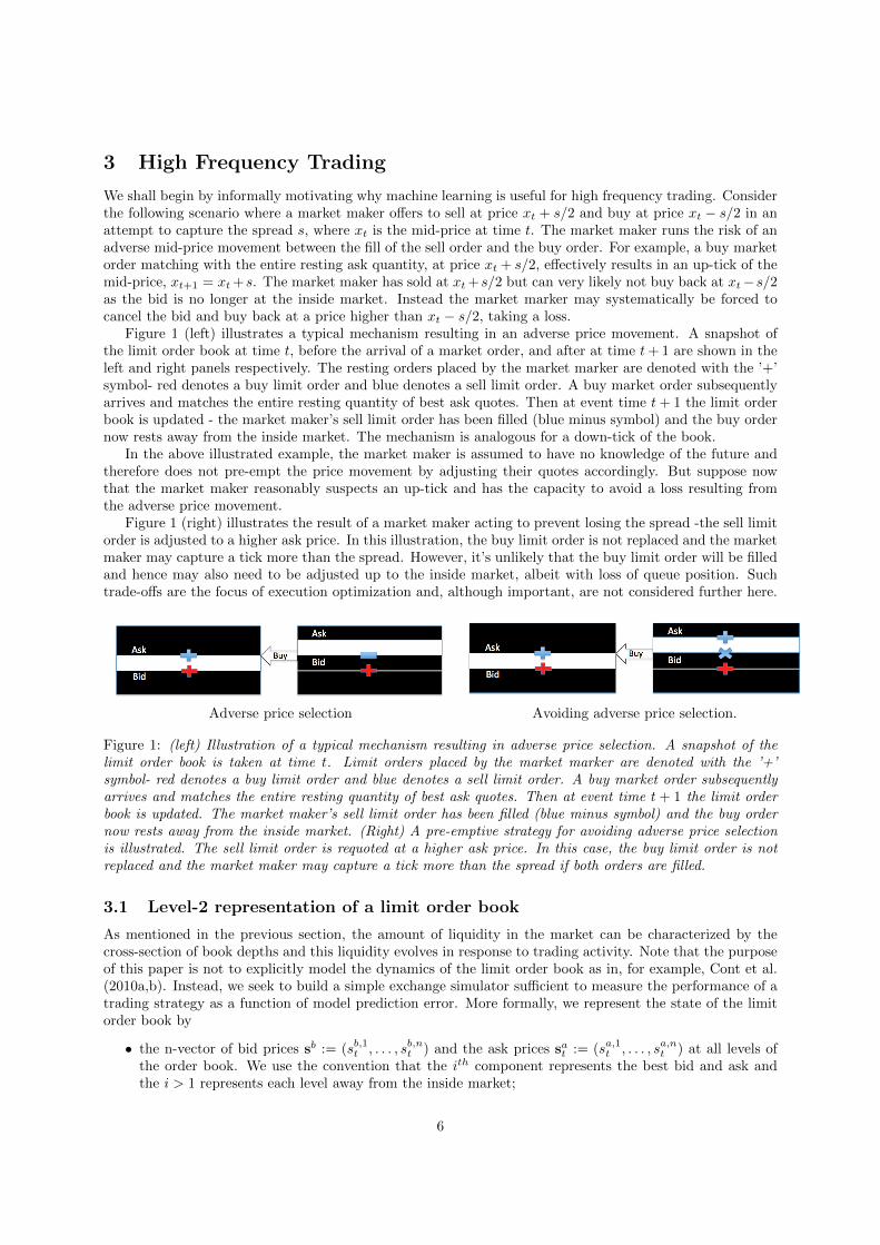
We shall begin by informally motivating why machine learning is useful for high frequency trading. Considerthe following scenario where a market maker offers to sell at price xt + s/2 and buy at price xt − s/2 in anattempt to capture the spread s, where xt is the mid-price at time t. The market maker runs the risk of anadverse mid-price movement between the fill of the sell order and the buy order. For example, a buy marketorder matching with the entire resting ask quantity, at price xt + s/2, effectively results in an up-tick of themid-price, xt+1 = xt+s. The market maker has sold at xt+s/2 but can very likely not buy back at xt−s/2as the bid is no longer at the inside market. Instead the market marker may systematically be forced tocancel the bid and buy back at a price higher than xt − s/2, taking a loss.

Figure 1 (left) illustrates a typical mechanism resulting in an adverse price movement. A snapshot ofthe limit order book at time t, before the arrival of a market order, and after at time t+ 1 are shown in theleft and right panels respectively. The resting orders placed by the market marker are denoted with the ’+’symbol- red denotes a buy limit order and blue denotes a sell limit order. A buy market order subsequentlyarrives and matches the entire resting quantity of best ask quotes. Then at event time t+ 1 the limit orderbook is updated - the market maker’s sell limit order has been filled (blue minus symbol) and the buy ordernow rests away from the inside market. The mechanism is analogous for a down-tick of the book.

In the above illustrated example, the market maker is assumed to have no knowledge of the future andtherefore does not pre-empt the price movement by adjusting their quotes accordingly. But suppose nowthat the market maker reasonably suspects an up-tick and has the capacity to avoid a loss resulting fromthe adverse price movement.

Figure 1 (right) illustrates the result of a market maker acting to prevent losing the spread -the sell limitorder is adjusted to a higher ask price. In this illustration, the buy limit order is not replaced and the marketmaker may capture a tick more than the spread. However, it’s unlikely that the buy limit order will be filledand hence may also need to be adjusted up to the inside market, albeit with loss of queue position. Suchtrade-offs are the focus of execution optimization and, although important, are not considered further here.

Adverse price selection Avoiding adverse price selection.

Figure 1: (left) Illustration of a typical mechanism resulting in adverse price selection. A snapshot of thelimit order book is taken at time t. Limit orders placed by the market marker are denoted with the ’+’symbol- red denotes a buy limit order and blue denotes a sell limit order. A buy market order subsequentlyarrives and matches the entire resting quantity of best ask quotes. Then at event time t + 1 the limit orderbook is updated. The market maker’s sell limit order has been filled (blue minus symbol) and the buy ordernow rests away from the inside market. (Right) A pre-emptive strategy for avoiding adverse price selectionis illustrated. The sell limit order is requoted at a higher ask price. In this case, the buy limit order is notreplaced and the market maker may capture a tick more than the spread if both orders are filled.

3.1 Level-2 representation of a limit order book

As mentioned in the previous section, the amount of liquidity in the market can be characterized by thecross-section of book depths and this liquidity evolves in response to trading activity. Note that the purposeof this paper is not to explicitly model the dynamics of the limit order book as in, for example, Cont et al.(2010a,b). Instead, we seek to build a simple exchange simulator sufficient to measure the performance of atrading strategy as a function of model prediction error. More formally, we represent the state of the limitorder book by

• the n-vector of bid prices sb := (sb,1t , . . . , sb,nt ) and the ask prices sat := (sa,1t , . . . , sa,nt ) at all levels ofthe order book. We use the convention that the ith component represents the best bid and ask andthe i > 1 represents each level away from the inside market;

6

• the n-vector of bid queues qbt := (qb,1, . . . , qb,nt ), where qb,it denotes the depth of each bid level i at timet; and

• the n-vector of ask queues qat := (qa,1, . . . , qa,nt ) where qa,it denotes the depth of each bid level i at timet.

The state of the limit order book is thus described by Xt := (sbt , sat ,q

bt ,q

at ) which takes values in the discrete

state space δ · Z2n × N2n for some tick size δ << 1. Note, for avoidance of doubt, that this notation stillpermits the bid-ask spread to change - this occurs when one or more of the price levels at the inside markethas zero depth.

The state Xt of the order book is modified by the following order book events arriving at time t:

• limit orders (at the bid or ask) of size Lbt := (Lb,1t , . . . , Lb,nt ) and Lat := (La,1t , . . . , La,nt );

• market orders (to buy or sell) of size M bt and Ms

t . These are referred to by practitioners as ’aggressors’;and

• cancelations of limit orders of size Cbt := (Cb,1t , . . . , Cb,nt ) and Ca

t := (Ca,1t , . . . , Ca,nt ).

When the bid or ask queue is depleted, the price moves up or down to the next level of the order book.More precisely,

1. When the best bid queue is depleted, the mid-price decreases by half a tick. The bid-ask spread istemporarily one and a half ticks;

2. Quotes subsequently arrive at a new lower ask level so that the bid-ask spread returns to a tick - themid-price has now decreased by another half-a-tick;

3. This full tick change in the mid-price, inclusive of the intermediate state, shall be referred to as a’price-down-flip’ or just ’price-flip’. Practitioner’s also use the terminology ’down-tick’ or the price issaid to ’tick-down’.

The converse mechanism, when the best ask queue is depleted, is referred to a ’price-up-flip’. Thefollowing example illustrates a price-down-flip in response to the arrival of a sell aggressor.

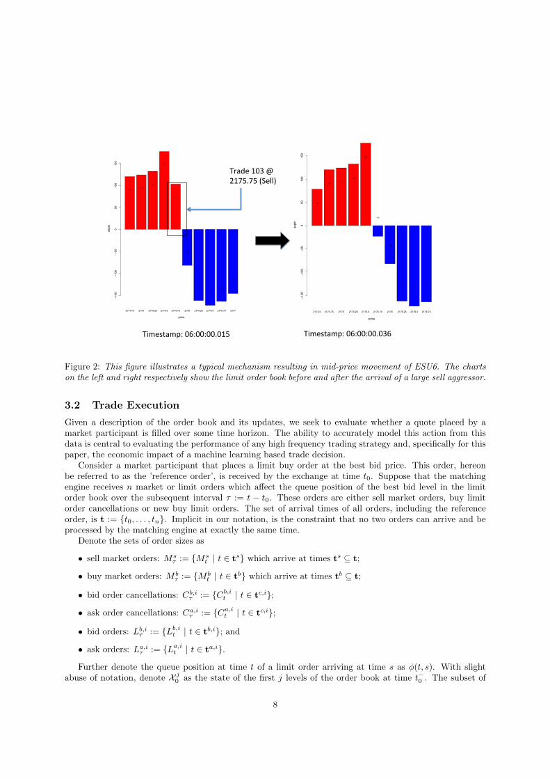
Example 1 (order book update). Figure 2 illustrates a typical mechanism resulting in mid-price movement.The charts on the left and right respectively show the limit order book of ESU6 before and after the arrivalof a large sell aggressor. The aggressor is sufficiently large to match all of the best bids. Once matched,the limit order is updated with a lower best bid of $2175.5. The gap between the best ask and best bid wouldwiden if it weren’t for the arrival of 23 new contracts offered at a lower ask price of $2175.75. The net effectis a full down-tick of the mid-price.

Using the notation introduced in this section, Table 1 records the limit order book before and after thearrival of the sell aggressor.

time X 1t Ms

t La,1tt0 (2175.75, 2176.0, 103, 82) 0 0t1 (2175.5, 2176.0, 177, 82) 103 0t2 (2175.5, 2175.75, 177, 23) 0 23

Table 1: This table shows the limit order book of ESU6 before and after the arrival of the sell aggressor, asillustrated in Figure 2.

The focus of the remainder of the paper is to develop and demonstrate a practical approach for measuringthe economic impact of the ability to predict these price-flips. We use machine learning to predict the pricemovements and then combine a simple model for estimating the queue position, fill execution, and for agiven market making strategy, estimate the expected P&L as a function of prediction error. The marketmaking strategy exploits predicted price movements.

7

2174.75 2175 2175.25 2175.5 2175.75 2176 2176.25 2176.5 2176.75 2177

price

depth

−150

−100

−50

050

100

150

120124

132

177

103

−82

−162

−173

−164

−146

2174.5 2174.75 2175 2175.25 2175.5 2175.75 2176 2176.25 2176.5 2176.75

price

depth

−150

−100

−50

050

100

150

78

120124

132

177

−23

−82

−162

−173

−164

Timestamp: 06:00:00.015 Timestamp: 06:00:00.036

Trade 103 @ 2175.75 (Sell)

Figure 2: This figure illustrates a typical mechanism resulting in mid-price movement of ESU6. The chartson the left and right respectively show the limit order book before and after the arrival of a large sell aggressor.

3.2 Trade Execution

Given a description of the order book and its updates, we seek to evaluate whether a quote placed by amarket participant is filled over some time horizon. The ability to accurately model this action from thisdata is central to evaluating the performance of any high frequency trading strategy and, specifically for thispaper, the economic impact of a machine learning based trade decision.

Consider a market participant that places a limit buy order at the best bid price. This order, hereonbe referred to as the ’reference order’, is received by the exchange at time t0. Suppose that the matchingengine receives n market or limit orders which affect the queue position of the best bid level in the limitorder book over the subsequent interval τ := t − t0. These orders are either sell market orders, buy limitorder cancellations or new buy limit orders. The set of arrival times of all orders, including the referenceorder, is t := t0, . . . , tn. Implicit in our notation, is the constraint that no two orders can arrive and beprocessed by the matching engine at exactly the same time.

Denote the sets of order sizes as

• sell market orders: Msτ := Ms

t | t ∈ ts which arrive at times ts ⊆ t;

• buy market orders: M bτ := M b

t | t ∈ tb which arrive at times tb ⊆ t;

• bid order cancellations: Cb,iτ := Cb,it | t ∈ tc,i;

• ask order cancellations: Ca,iτ := Ca,it | t ∈ tc,i;

• bid orders: Lb,iτ := Lb,it | t ∈ tb,i; and

• ask orders: La,iτ := La,it | t ∈ ta,i.

Further denote the queue position at time t of a limit order arriving at time s as φ(t, s). With slightabuse of notation, denote X j0 as the state of the first j levels of the order book at time t−0 . The subset of

8

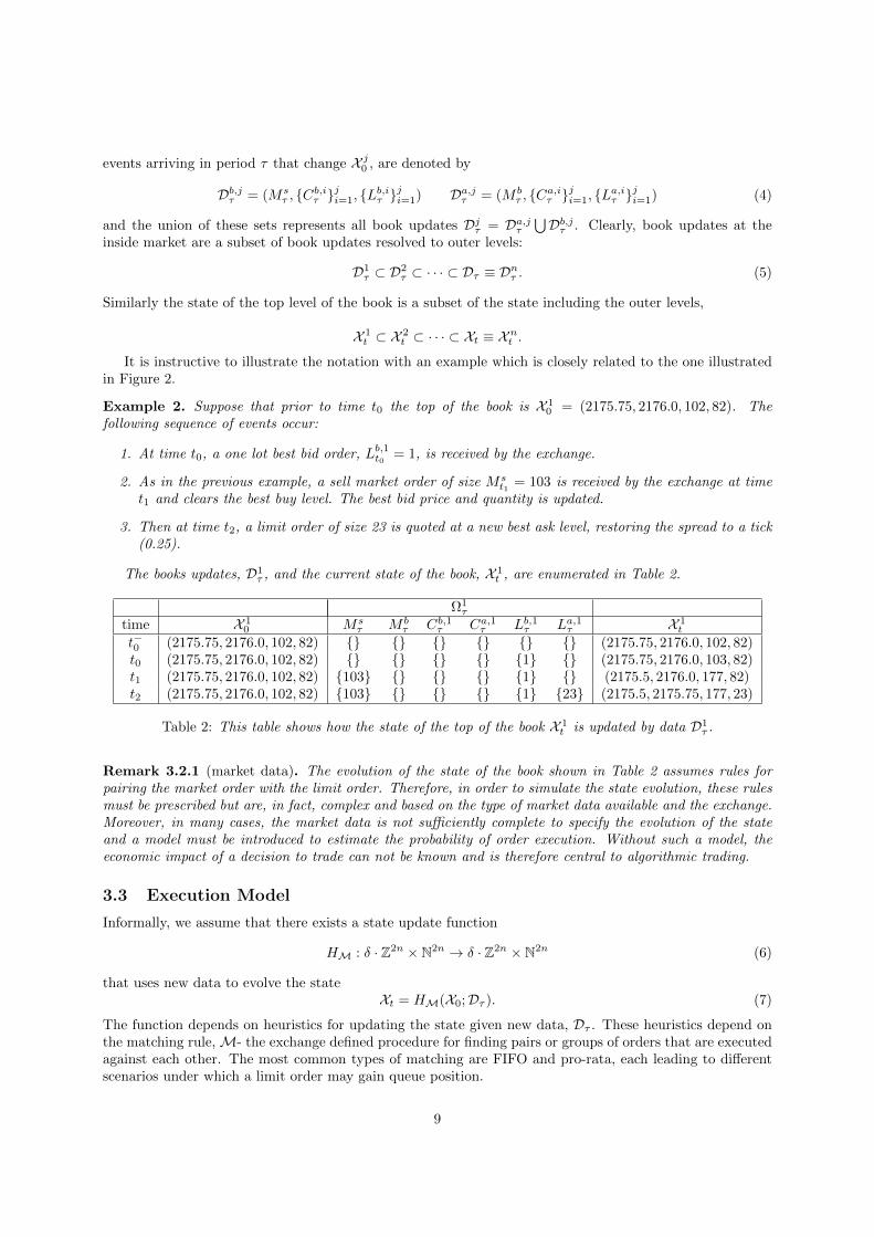
events arriving in period τ that change X j0 , are denoted by

Db,jτ = (Msτ , Cb,iτ ji=1, Lb,iτ ji=1) Da,jτ = (M b

τ , Ca,iτ ji=1, La,iτ ji=1) (4)

and the union of these sets represents all book updates Djτ = Da,jτ⋃Db,jτ . Clearly, book updates at the

inside market are a subset of book updates resolved to outer levels:

D1τ ⊂ D2

τ ⊂ · · · ⊂ Dτ ≡ Dnτ . (5)

Similarly the state of the top level of the book is a subset of the state including the outer levels,

X 1t ⊂ X 2

t ⊂ · · · ⊂ Xt ≡ Xnt .It is instructive to illustrate the notation with an example which is closely related to the one illustrated

in Figure 2.

Example 2. Suppose that prior to time t0 the top of the book is X 10 = (2175.75, 2176.0, 102, 82). The

following sequence of events occur:

1. At time t0, a one lot best bid order, Lb,1t0 = 1, is received by the exchange.

2. As in the previous example, a sell market order of size Mst1 = 103 is received by the exchange at time

t1 and clears the best buy level. The best bid price and quantity is updated.

3. Then at time t2, a limit order of size 23 is quoted at a new best ask level, restoring the spread to a tick(0.25).

The books updates, D1τ , and the current state of the book, X 1

t , are enumerated in Table 2.

Ω1τ

time X 10 Ms

τ M bτ Cb,1τ Ca,1τ Lb,1τ La,1τ X 1

t

t−0 (2175.75, 2176.0, 102, 82) (2175.75, 2176.0, 102, 82)t0 (2175.75, 2176.0, 102, 82) 1 (2175.75, 2176.0, 103, 82)t1 (2175.75, 2176.0, 102, 82) 103 1 (2175.5, 2176.0, 177, 82)t2 (2175.75, 2176.0, 102, 82) 103 1 23 (2175.5, 2175.75, 177, 23)

Table 2: This table shows how the state of the top of the book X 1t is updated by data D1

τ .

Remark 3.2.1 (market data). The evolution of the state of the book shown in Table 2 assumes rules forpairing the market order with the limit order. Therefore, in order to simulate the state evolution, these rulesmust be prescribed but are, in fact, complex and based on the type of market data available and the exchange.Moreover, in many cases, the market data is not sufficiently complete to specify the evolution of the stateand a model must be introduced to estimate the probability of order execution. Without such a model, theeconomic impact of a decision to trade can not be known and is therefore central to algorithmic trading.

3.3 Execution Model

Informally, we assume that there exists a state update function

HM : δ · Z2n × N2n → δ · Z2n × N2n (6)

that uses new data to evolve the stateXt = HM(X0;Dτ ). (7)

The function depends on heuristics for updating the state given new data, Dτ . These heuristics depend onthe matching rule,M- the exchange defined procedure for finding pairs or groups of orders that are executedagainst each other. The most common types of matching are FIFO and pro-rata, each leading to differentscenarios under which a limit order may gain queue position.

9

We shall assume that queue position of a limit order place at time s is given by a function φs : R+×Z→ N,so that φt,s := φt(Ls;Xs−,Dτ ) gives its queue position at time t ≥ s. These matching rules are different foreach exchange and are occasionally updated.The reference bid (or ask) order L0 received by the exchange at time t0 is filled (a.k.a. executed) by time tnif both criteria are met:

1. All bids (respectively offers) at the best level in the limit order book with higher queue priority areeither cancelled or all these higher priority limit orders, including the reference order, are matchedwith one or more sell (respectively buy) aggressors arriving over the interval τ . Our order is partiallyfilled if, under the same set of events, the exchange only matches a portion of the reference order.

2. Any reference order cancellation is not received at or before time tn.

We quantify the extent to which L0 is filled given the triple (L0,X0,Dτ ). Since the queue position of L0

in unknown, we introduce a parameterization representing the degree of conservativeness in order execution.We introduce the trade-to-book ratio as a measure of the trade size relative to resting quantity in front ofand including an order placed at time t0. This ratio is scaled so that a value of at least unity indicates acomplete fill. Otherwise, the ratio indicates that the current trade size is inadequate to completely fill theorder. It is further possible to determine the lower bound corresponding to a partial fill of the referenceorder.

Definition 3.3.1 (Trade-to-Book Ratio). In the event of a sell market order arriving at time t, the trade-

to-book ratio of a level j bid limit order, Lb,j0 , placed at time t0 is a function R : R+ × N → R+ of theform

Rt(Lb,j0 ;Db,jτ , ω) =Mst

Qb,j0 −(∑

u∈ts Msu + ω

∑ji=1

∑u∈tc,i C

b,iu −

∑ji=1

∑t∈tb,i 1φu,u<φu,t0

Lb,iu

) (8)

where

• Qb,j0 :=∑ji=1 q

b,it0 denotes the sum of the depths of the queue at time t0 up to the jth bid level;

• ∑u∈ts Msu are subsequent set of sell market orders arriving at times ts;

• ∑u∈tc,i Cb,iu is the subsequent of level i bid orders cancelled at times tc,i;

• 1φu,u<φu,t0 is an indicator function returning unity if a subsequent limit order placed at time u hashigher queue priority than the time t0 reference limit order; and

• ω ∈ [0, 1] is an unknown cancellation parameter which denotes the proportion of cancellations of orderswith higher queue priority than the reference limit order over the interval τ . ω = 1 represents the mostfavorable scenario where all cancellations result in an advancement of queue position and ω = 0 theconverse.

Remark 3.3.2 (market-by-order data). If market-by-order data is available, then Dτ contains a richer setof information that can be used to exactly determine the queue position of a cancelled limit order. Then theparameter ω can be replaced by the indicator function 1φu,u<φu,t0 (placed inside the summation operator)and no approximation is needed.

It is instructive to view numerical examples of the trade-to-book ratio estimation, under either FIFOor pro-rata matching rules. These examples assume full view of the limit orders at the best buy level.Depending on the market, the size of each order may not be not known, only the total resting quantity andnumber of orders at the price level can typically be extracted from the market data feeds.

Example 3 (FIFO market). Suppose at time t−0 the queue depth at the best bid is 50. The reference limitorder to buy 50 contracts at the best bid level is received by the exchange at time t0. In a FIFO market, thelimit order joins the back of the queue at the best bid level. Let’s further suppose that between time t0 andtime t a market sell order of size 25 subsequently arrives. Additionally, in this time interval, a best bid limit

10

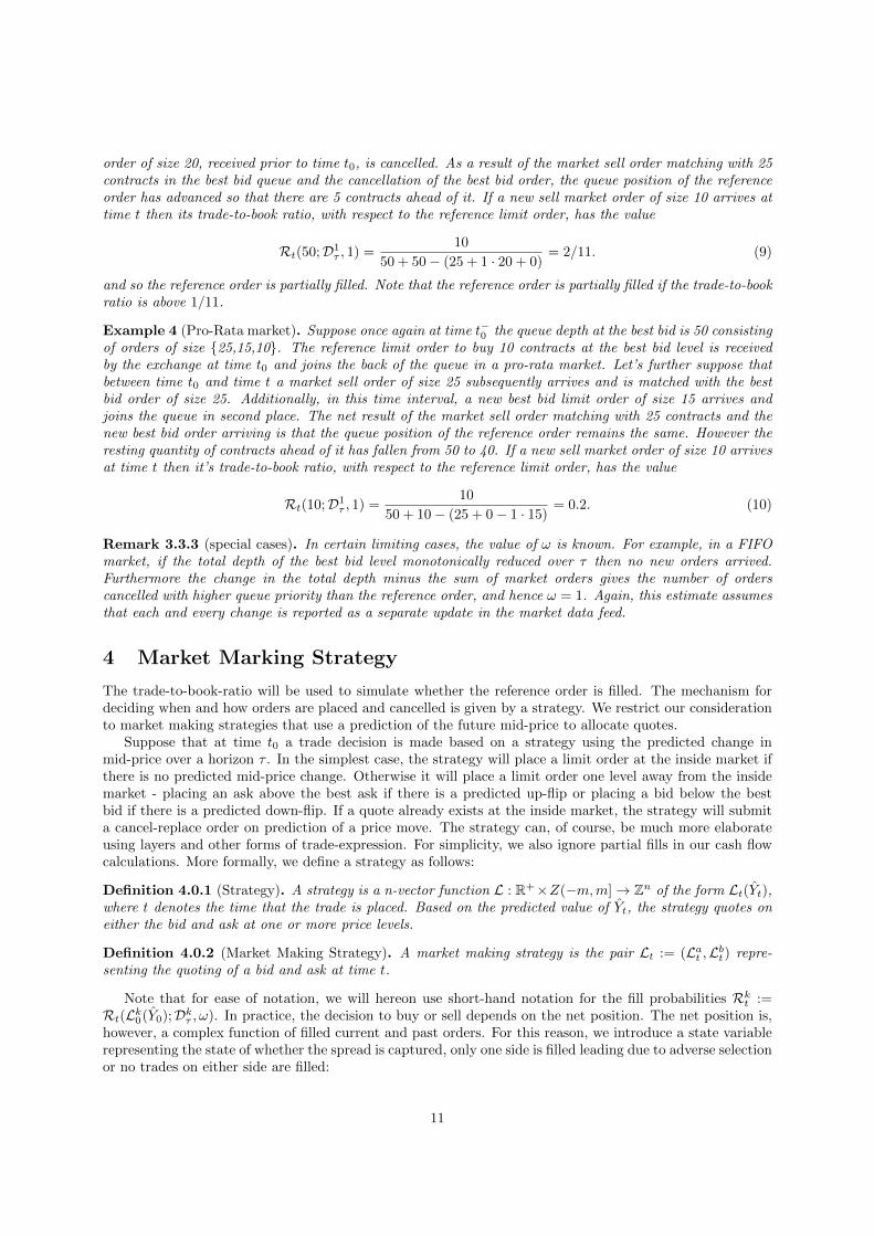
order of size 20, received prior to time t0, is cancelled. As a result of the market sell order matching with 25contracts in the best bid queue and the cancellation of the best bid order, the queue position of the referenceorder has advanced so that there are 5 contracts ahead of it. If a new sell market order of size 10 arrives attime t then its trade-to-book ratio, with respect to the reference limit order, has the value

Rt(50;D1τ , 1) =

10

50 + 50− (25 + 1 · 20 + 0)= 2/11. (9)

and so the reference order is partially filled. Note that the reference order is partially filled if the trade-to-bookratio is above 1/11.

Example 4 (Pro-Rata market). Suppose once again at time t−0 the queue depth at the best bid is 50 consistingof orders of size 25,15,10. The reference limit order to buy 10 contracts at the best bid level is receivedby the exchange at time t0 and joins the back of the queue in a pro-rata market. Let’s further suppose thatbetween time t0 and time t a market sell order of size 25 subsequently arrives and is matched with the bestbid order of size 25. Additionally, in this time interval, a new best bid limit order of size 15 arrives andjoins the queue in second place. The net result of the market sell order matching with 25 contracts and thenew best bid order arriving is that the queue position of the reference order remains the same. However theresting quantity of contracts ahead of it has fallen from 50 to 40. If a new sell market order of size 10 arrivesat time t then it’s trade-to-book ratio, with respect to the reference limit order, has the value

Rt(10;D1τ , 1) =

10

50 + 10− (25 + 0− 1 · 15)= 0.2. (10)

Remark 3.3.3 (special cases). In certain limiting cases, the value of ω is known. For example, in a FIFOmarket, if the total depth of the best bid level monotonically reduced over τ then no new orders arrived.Furthermore the change in the total depth minus the sum of market orders gives the number of orderscancelled with higher queue priority than the reference order, and hence ω = 1. Again, this estimate assumesthat each and every change is reported as a separate update in the market data feed.

4 Market Marking Strategy

The trade-to-book-ratio will be used to simulate whether the reference order is filled. The mechanism fordeciding when and how orders are placed and cancelled is given by a strategy. We restrict our considerationto market making strategies that use a prediction of the future mid-price to allocate quotes.

Suppose that at time t0 a trade decision is made based on a strategy using the predicted change inmid-price over a horizon τ . In the simplest case, the strategy will place a limit order at the inside market ifthere is no predicted mid-price change. Otherwise it will place a limit order one level away from the insidemarket - placing an ask above the best ask if there is a predicted up-flip or placing a bid below the bestbid if there is a predicted down-flip. If a quote already exists at the inside market, the strategy will submita cancel-replace order on prediction of a price move. The strategy can, of course, be much more elaborateusing layers and other forms of trade-expression. For simplicity, we also ignore partial fills in our cash flowcalculations. More formally, we define a strategy as follows:

Definition 4.0.1 (Strategy). A strategy is a n-vector function L : R+×Z(−m,m]→ Zn of the form Lt(Yt),where t denotes the time that the trade is placed. Based on the predicted value of Yt, the strategy quotes oneither the bid and ask at one or more price levels.

Definition 4.0.2 (Market Making Strategy). A market making strategy is the pair Lt := (Lat ,Lbt) repre-senting the quoting of a bid and ask at time t.

Note that for ease of notation, we will hereon use short-hand notation for the fill probabilities Rkt :=Rt(Lk0(Y0);Dkτ , ω). In practice, the decision to buy or sell depends on the net position. The net position is,however, a complex function of filled current and past orders. For this reason, we introduce a state variablerepresenting the state of whether the spread is captured, only one side is filled leading due to adverse selectionor no trades on either side are filled:

11

Definition 4.0.3 (Spread State). The state of the spread at time t based on the market making strategy L0

is a function Z : [−1, 1] ∩ Z→ [−1, 1] ∩ Z of the form

Zt(Y0) =

1, A :=⋃nk=1R

k,at ≥ 1 ∩⋃nk=1R

k,bt ≥ 1 6= ∅,

−1, B :=⋃nk=1R

k,at < 1 ∩⋃nk=1R

k,bt < 1 6= ∅,

0, (A ∪B)c 6= ∅.(11)

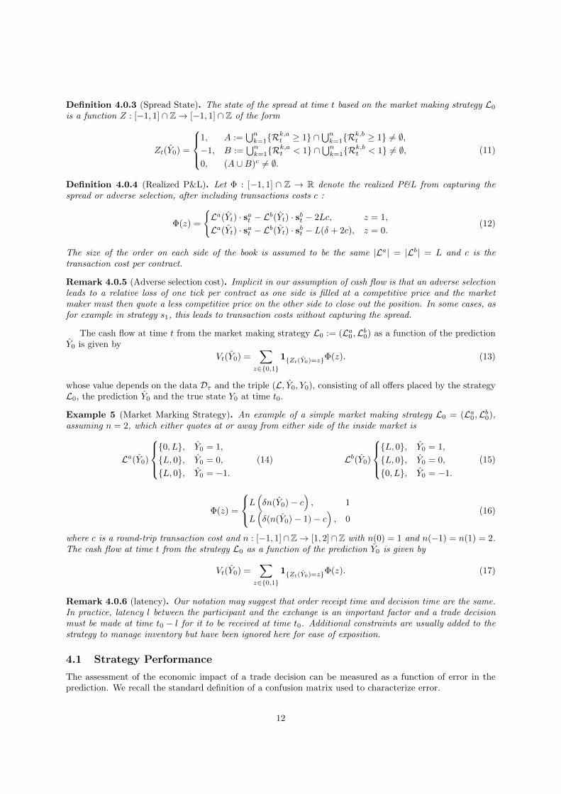
Definition 4.0.4 (Realized P&L). Let Φ : [−1, 1] ∩ Z → R denote the realized P&L from capturing thespread or adverse selection, after including transactions costs c :

Φ(z) =

La(Yt) · sat − Lb(Yt) · sbt − 2Lc, z = 1,

La(Yt) · sat − Lb(Yt) · sbt − L(δ + 2c), z = 0.(12)

The size of the order on each side of the book is assumed to be the same |La| = |Lb| = L and c is thetransaction cost per contract.

Remark 4.0.5 (Adverse selection cost). Implicit in our assumption of cash flow is that an adverse selectionleads to a relative loss of one tick per contract as one side is filled at a competitive price and the marketmaker must then quote a less competitive price on the other side to close out the position. In some cases, asfor example in strategy s1, this leads to transaction costs without capturing the spread.

The cash flow at time t from the market making strategy L0 := (La0 ,Lb0) as a function of the predictionY0 is given by

Vt(Y0) =∑

z∈0,11Zt(Y0)=zΦ(z). (13)

whose value depends on the data Dτ and the triple (L, Y0, Y0), consisting of all offers placed by the strategyL0, the prediction Y0 and the true state Y0 at time t0.

Example 5 (Market Marking Strategy). An example of a simple market making strategy L0 = (La0 ,Lb0),assuming n = 2, which either quotes at or away from either side of the inside market is

La(Y0)

0, L, Y0 = 1,

L, 0, Y0 = 0,

L, 0, Y0 = −1.

(14) Lb(Y0)

L, 0, Y0 = 1,

L, 0, Y0 = 0,

0, L, Y0 = −1.

(15)

Φ(z) =

L(δn(Y0)− c

), 1

L(δ(n(Y0)− 1)− c

), 0

(16)

where c is a round-trip transaction cost and n : [−1, 1]∩Z→ [1, 2]∩Z with n(0) = 1 and n(−1) = n(1) = 2.The cash flow at time t from the strategy L0 as a function of the prediction Y0 is given by

Vt(Y0) =∑

z∈0,11Zt(Y0)=zΦ(z). (17)

Remark 4.0.6 (latency). Our notation may suggest that order receipt time and decision time are the same.In practice, latency l between the participant and the exchange is an important factor and a trade decisionmust be made at time t0 − l for it to be received at time t0. Additional constraints are usually added to thestrategy to manage inventory but have been ignored here for ease of exposition.

4.1 Strategy Performance

The assessment of the economic impact of a trade decision can be measured as a function of error in theprediction. We recall the standard definition of a confusion matrix used to characterize error.

12

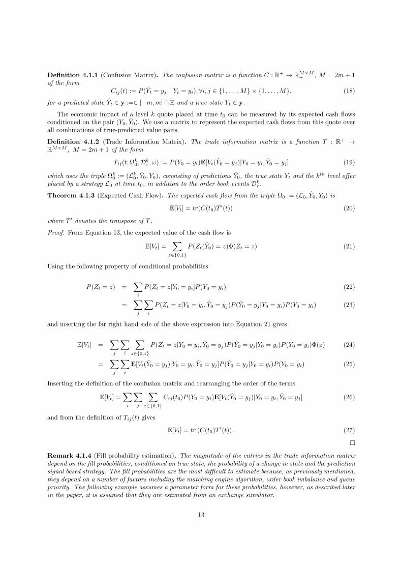
Definition 4.1.1 (Confusion Matrix). The confusion matrix is a function C : R+ → RM×M+ , M = 2m+ 1of the form

Cij(t) := P (Yt = yj | Yt = yi),∀i, j ∈ 1, . . . ,M × 1, . . . ,M, (18)

for a predicted state Yt ∈ y :=∈ [−m,m] ∩ Z and a true state Yt ∈ y.

The economic impact of a level k quote placed at time t0 can be measured by its expected cash flowsconditioned on the pair (Y0, Y0). We use a matrix to represent the expected cash flows from this quote overall combinations of true-predicted value pairs.

Definition 4.1.2 (Trade Information Matrix). The trade information matrix is a function T : R+ →RM×M , M = 2m+ 1 of the form

Tij(t; Ωk0 ,Dkτ , ω) := P (Y0 = yi)E[Vt(Y0 = yj)|Y0 = yi, Y0 = yj ] (19)

which uses the triple Ωk0 := (Lk0 , Y0, Y0), consisting of predictions Y0, the true state Yt and the kth level offerplaced by a strategy L0 at time t0, in addition to the order book events Dkτ .

Theorem 4.1.3 (Expected Cash Flow). The expected cash flow from the triple Ω0 := (L0, Y0, Y0) is

E[Vt] = tr(C(t0)T ′(t)) (20)

where T ′ denotes the transpose of T .

Proof. From Equation 13, the expected value of the cash flow is

E[Vt] =∑

z∈0,1P (Zt(Y0) = z)Φ(Zt = z) (21)

Using the following property of conditional probabilities

P (Zt = z) =∑

i

P (Zt = z|Y0 = yi]P (Y0 = yi) (22)

=∑

j

∑

i

P (Zt = z|Y0 = yi, Y0 = yj)P (Y0 = yj |Y0 = yi)P (Y0 = yi) (23)

and inserting the far right hand side of the above expression into Equation 21 gives

E[Vt] =∑

j

∑

i

∑

z∈0,1P (Zt = z|Y0 = yi, Y0 = yj)P (Y0 = yj |Y0 = yi)P (Y0 = yi)Φ(z) (24)

=∑

j

∑

i

E[Vt(Y0 = yj)|Y0 = yi, Y0 = yj ]P (Y0 = yj |Y0 = yi)P (Y0 = yi) (25)

Inserting the definition of the confusion matrix and rearranging the order of the terms

E[Vt] =∑

i

∑

j

∑

z∈0,1Cij(t0)P (Y0 = yi)E[Vt(Y0 = yj)|Y0 = yi, Y0 = yj ] (26)

and from the definition of Tij(t) gives

E[Vt] = tr (C(t0)T ′(t)) . (27)

Remark 4.1.4 (Fill probability estimation). The magnitude of the entries in the trade information matrixdepend on the fill probabilities, conditioned on true state, the probability of a change in state and the predictionsignal based strategy. The fill probabilities are the most difficult to estimate because, as previously mentioned,they depend on a number of factors including the matching engine algorithm, order book imbalance and queuepriority. The following example assumes a parameter form for these probabilities, however, as described laterin the paper, it is assumed that they are estimated from an exchange simulator.

13

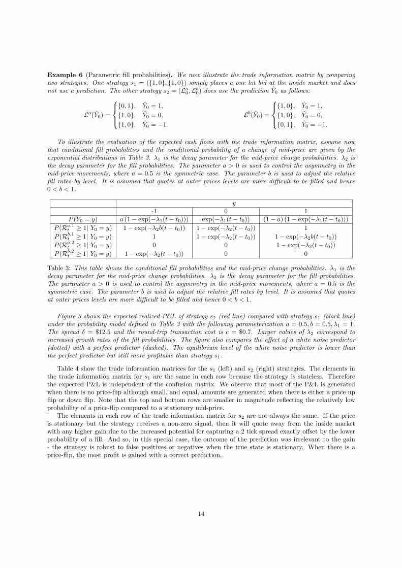
Example 6 (Parametric fill probabilities). We now illustrate the trade information matrix by comparingtwo strategies. One strategy s1 = (1, 0, 1, 0) simply places a one lot bid at the inside market and doesnot use a prediction. The other strategy s2 = (La0 ,Lb0) does use the prediction Y0 as follows:

La(Y0) =

0, 1, Y0 = 1,

1, 0, Y0 = 0,

1, 0, Y0 = −1.

Lb(Y0) =

1, 0, Y0 = 1,

1, 0, Y0 = 0,

0, 1, Y0 = −1.

To illustrate the evaluation of the expected cash flows with the trade information matrix, assume nowthat conditional fill probabilities and the conditional probability of a change of mid-price are given by theexponential distributions in Table 3. λ1 is the decay parameter for the mid-price change probabilities. λ2 isthe decay parameter for the fill probabilities. The parameter a > 0 is used to control the asymmetry in themid-price movements, where a = 0.5 is the symmetric case. The parameter b is used to adjust the relativefill rates by level. It is assumed that quotes at outer prices levels are more difficult to be filled and hence0 < b < 1.

y-1 0 1

P (Y0 = y) a (1− exp(−λ1(t− t0))) exp(−λ1(t− t0)) (1− a) (1− exp(−λ1(t− t0)))

P (Ra,1t ≥ 1| Y0 = y) 1− exp(−λ2b(t− t0)) 1− exp(−λ2(t− t0)) 1

P (Rb,1t ≥ 1| Y0 = y) 1 1− exp(−λ2(t− t0)) 1− exp(−λ2b(t− t0))

P (Ra,2t ≥ 1| Y0 = y) 0 0 1− exp(−λ2(t− t0))

P (Rb,2t ≥ 1| Y0 = y) 1− exp(−λ2(t− t0)) 0 0

Table 3: This table shows the conditional fill probabilities and the mid-price change probabilities. λ1 is thedecay parameter for the mid-price change probabilities. λ2 is the decay parameter for the fill probabilities.The parameter a > 0 is used to control the asymmetry in the mid-price movements, where a = 0.5 is thesymmetric case. The parameter b is used to adjust the relative fill rates by level. It is assumed that quotesat outer prices levels are more difficult to be filled and hence 0 < b < 1.

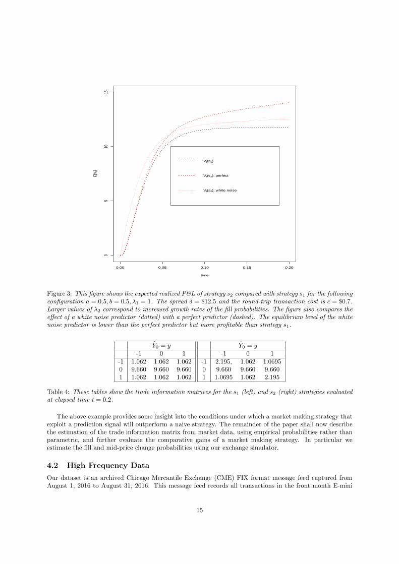
Figure 3 shows the expected realized P&L of strategy s2 (red line) compared with strategy s1 (black line)under the probability model defined in Table 3 with the following parameterization a = 0.5, b = 0.5, λ1 = 1.The spread δ = $12.5 and the round-trip transaction cost is c = $0.7. Larger values of λ2 correspond toincreased growth rates of the fill probabilities. The figure also compares the effect of a white noise predictor(dotted) with a perfect predictor (dashed). The equilibrium level of the white noise predictor is lower thanthe perfect predictor but still more profitable than strategy s1.

Table 4 show the trade information matrices for the s1 (left) and s2 (right) strategies. The elements inthe trade information matrix for s1 are the same in each row because the strategy is stateless. Thereforethe expected P&L is independent of the confusion matrix. We observe that most of the P&L is generatedwhen there is no price-flip although small, and equal, amounts are generated when there is either a price upflip or down flip. Note that the top and bottom rows are smaller in magnitude reflecting the relatively lowprobability of a price-flip compared to a stationary mid-price.

The elements in each row of the trade information matrix for s2 are not always the same. If the priceis stationary but the strategy receives a non-zero signal, then it will quote away from the inside marketwith any higher gain due to the increased potential for capturing a 2 tick spread exactly offset by the lowerprobability of a fill. And so, in this special case, the outcome of the prediction was irrelevant to the gain- the strategy is robust to false positives or negatives when the true state is stationary. When there is aprice-flip, the most profit is gained with a correct prediction.

14

0.00 0.05 0.10 0.15 0.20

05

1015

time

E[V t

]

Vt(s1)

Vt(s2): perfect

Vt(s2): white noise

Figure 3: This figure shows the expected realized P&L of strategy s2 compared with strategy s1 for the followingconfiguration a = 0.5, b = 0.5, λ1 = 1. The spread δ = $12.5 and the round-trip transaction cost is c = $0.7.Larger values of λ2 correspond to increased growth rates of the fill probabilities. The figure also compares theeffect of a white noise predictor (dotted) with a perfect predictor (dashed). The equilibrium level of the whitenoise predictor is lower than the perfect predictor but more profitable than strategy s1.

Y0 = y-1 0 1

-1 1.062 1.062 1.0620 9.660 9.660 9.6601 1.062 1.062 1.062

Y0 = y-1 0 1

-1 2.195, 1.062 1.06950 9.660 9.660 9.6601 1.0695 1.062 2.195

Table 4: These tables show the trade information matrices for the s1 (left) and s2 (right) strategies evaluatedat elapsed time t = 0.2.

The above example provides some insight into the conditions under which a market making strategy thatexploit a prediction signal will outperform a naive strategy. The remainder of the paper shall now describethe estimation of the trade information matrix from market data, using empirical probabilities rather thanparametric, and further evaluate the comparative gains of a market making strategy. In particular weestimate the fill and mid-price change probabilities using our exchange simulator.

4.2 High Frequency Data

Our dataset is an archived Chicago Mercantile Exchange (CME) FIX format message feed captured fromAugust 1, 2016 to August 31, 2016. This message feed records all transactions in the front month E-mini

15

S&P 500 futures contract (ESU6) between the times of 12:00pm and 22:00 UTC. The ES tick size is a quarterof a point, or 12.50 per contract (rounded to the nearest cent). We extract details of each limit order bookupdate, including the nano-second resolution time-stamp, the quoted price and depth for each limit orderbook level.

The mid-price at time t is denoted by

pt =sa,1t + sb,1t

2. (28)

This mid-price can evolve in minimum increments of half a tick but is almost always observed to move atincrements of a tick over time intervals of a milli-second or less. In our feature set, each limit order bookupdate is recorded as an observation. Each observation is labelled based on whether the mid-price willincrease, decrease or remain constant over a horizon h:

Yt = ∆ptt+h, (29)

where ∆ptt+h is the forecast of discrete mid-price changes from time t to t + h, given measurement of thepredictors up to time t. The forecasting horizon h can be chosen to represent a fixed number of events orcan be a fixed time interval. This choice is based on practical considerations which are discussed later inSection 5.

Table 5 shows the limit order book before and after the arrival of the sell aggressor. Here, the responseYt is mid-price movement, in units of ticks, between the current and next tick.

Timestamp sb,1t sb,2t . . . qb,1t qb,2t . . . sa,1t sa,2t . . . qa,1t qa,2t . . . Yt06:00:00.015 2175.75 2175.5 . . . 103 177 . . . 2176 2176.25 . . . 82 162 . . . -106:00:00.036 2175.5 2175.25 . . . 177 132 . . . 2175.75 2176 . . . 23 82 . . . 0

Table 5: This table shows the limit order book of ESU6 before and after the arrival of the sell aggressor listedin Figure 2. Here, the response is the mid-price movement over the subsequent interval, in units of ticks. sb,itand qb,it denote the level i quoted bid price and depth of the limit order book at time t. sa,it and qa,it denotethe corresponding level i quoted ask price and depth.

The result of categorizing (a.k.a. labeling) each observation leads to a class imbalance problem as, at sucha short prediction horizon, approximately 99% of the observations have a zero response. To construct a ’bal-anced’ training set, observations (sequences of input variables) labeled by the minority class are oversampledwith replacement and the majority class observations are undersampled without replacement.

Following Kercheval and Zhang (2015); Sirignano (2016); Dixon (2017), we compose our feature set offive levels of prices, volumes and number of limit orders on both the ask and bid side of the book. Weadditionally, and somewhat heuristically via a process of ’feature engineering’, characterize order flow bythe ratio of the number of market buy orders arriving in the prior 50 observations to the resting number ofask limit orders at the top of book. We construct the analogous ratio for the sell by orders. This rationalefor this ratio is motivated by our observation that an increase in this ratio will more likely deplete the bestask level and the mid-price will up-tick, and vice-versa for a down-tick. The combination of this spatialrepresentation of the limit order book and the order flow gives a total of P = 32 features.

5 Results

The exact architecture and weight matrix sizes of our recurrent neural network are given by

output : Y k = softmax(F ky (hT )) =exp(F ky (hT ))

∑Kj=1 exp(F jy (hT ))

,

hidden states : ht = max (WhXt + Uhht−1 + bh, 0) , t = 1, . . . , T,

where Wh ∈ R20×32, Uh ∈ R20×20 and Wy ∈ R3×20. We initialize the hidden states to zero. We use theSGD method, implemented in Python’s TensorFlow Abadi et al. (2016) framework, to find the optimal

16

network weights, bias terms and regularization parameters. We employ an exponentially decaying learningrate schedule with an initial value of 10−2. The optimal `2 regularization is found, via a grid-search, to beλ2 = 0.01. The Glorot and Bengio method is used to initialize the weights of the network Glorot and Bengio(2010).

Times series cross-validation is performed over 20 consecutive trading days. Training sets are compiledfrom the previous 3 trading days and contain, on average, 5, 192, 822 observations. These sets are balancedresulting in a reduced training set size of typically just less than 100, 000 observations. The validation andtest sets are compiled for the next trading day following the 3 day training period. These are unbalanced,with the verification set containing 2× 105 observations and the remaining test set, on average, containingapproximately 1.5× 106 observations. Each experiment is run for 1000 epochs with a mini-batch size of 500drawn from the training set of 32 input variables. We follow the standard convention of choosing the numberof epochs based on convergence of the cross-entropy and the mini-batch size is chosen for computationalperformance. Each sequence is chosen to be of length 10 and the number of hidden units is chosen between10 and 20. The gridded search to find the optimal network architecture and regularization parameters takesseveral hours on a modern graphics processing unit (GPU). The search yields several candidate architecturesand parameter values.

To reliably measure performance on the unbalanced test set, we compute the F1 score - the geometricmean of the precision and recall:

F1 = 2precision · recall

precision + recall.

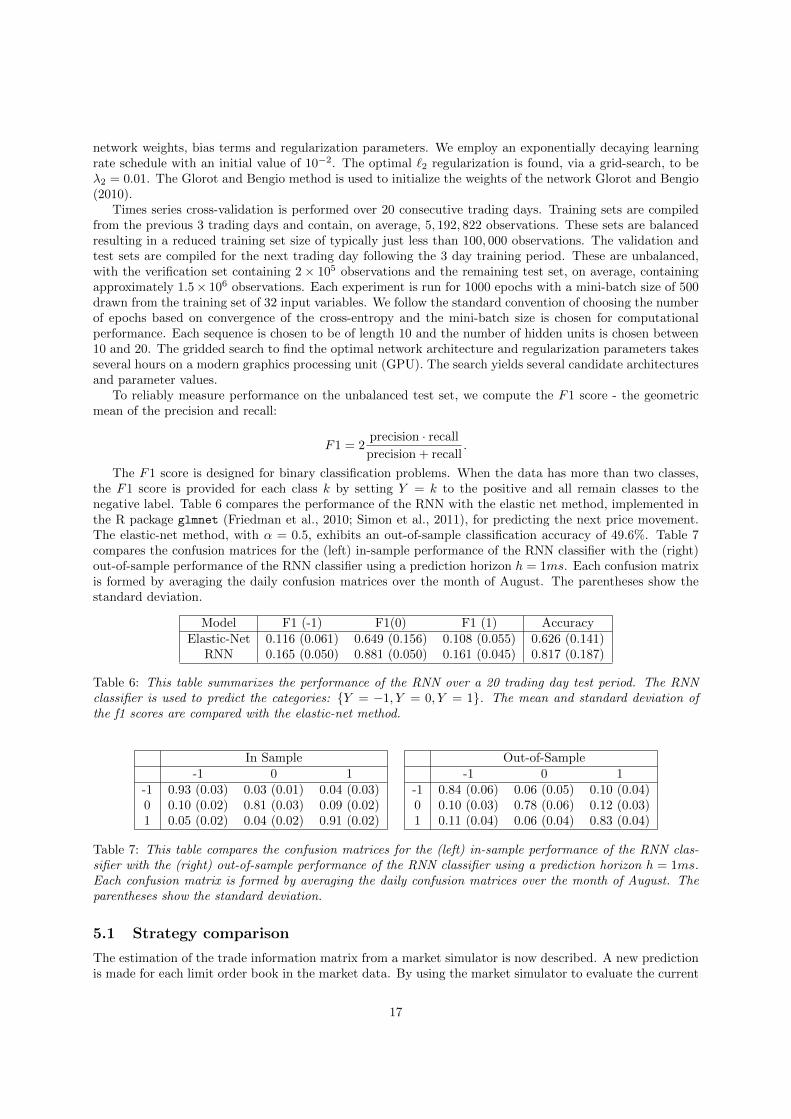
The F1 score is designed for binary classification problems. When the data has more than two classes,the F1 score is provided for each class k by setting Y = k to the positive and all remain classes to thenegative label. Table 6 compares the performance of the RNN with the elastic net method, implemented inthe R package glmnet (Friedman et al., 2010; Simon et al., 2011), for predicting the next price movement.The elastic-net method, with α = 0.5, exhibits an out-of-sample classification accuracy of 49.6%. Table 7compares the confusion matrices for the (left) in-sample performance of the RNN classifier with the (right)out-of-sample performance of the RNN classifier using a prediction horizon h = 1ms. Each confusion matrixis formed by averaging the daily confusion matrices over the month of August. The parentheses show thestandard deviation.

Model F1 (-1) F1(0) F1 (1) AccuracyElastic-Net 0.116 (0.061) 0.649 (0.156) 0.108 (0.055) 0.626 (0.141)

RNN 0.165 (0.050) 0.881 (0.050) 0.161 (0.045) 0.817 (0.187)

Table 6: This table summarizes the performance of the RNN over a 20 trading day test period. The RNNclassifier is used to predict the categories: Y = −1, Y = 0, Y = 1. The mean and standard deviation ofthe f1 scores are compared with the elastic-net method.

In Sample-1 0 1

-1 0.93 (0.03) 0.03 (0.01) 0.04 (0.03)0 0.10 (0.02) 0.81 (0.03) 0.09 (0.02)1 0.05 (0.02) 0.04 (0.02) 0.91 (0.02)

Out-of-Sample-1 0 1

-1 0.84 (0.06) 0.06 (0.05) 0.10 (0.04)0 0.10 (0.03) 0.78 (0.06) 0.12 (0.03)1 0.11 (0.04) 0.06 (0.04) 0.83 (0.04)

Table 7: This table compares the confusion matrices for the (left) in-sample performance of the RNN clas-sifier with the (right) out-of-sample performance of the RNN classifier using a prediction horizon h = 1ms.Each confusion matrix is formed by averaging the daily confusion matrices over the month of August. Theparentheses show the standard deviation.

5.1 Strategy comparison

The estimation of the trade information matrix from a market simulator is now described. A new predictionis made for each limit order book in the market data. By using the market simulator to evaluate the current

17

position, a market making strategy will typically quote to maintain a target position and remain withinan inventory constraint. A prediction based market marking strategy will additionally adjust the quote ifthe prediction changes, even if the overall position hasn’t changed since the previous book update. In ourexperiments, we update the quotes at the end of each prediction horizon which has been chosen to be h = 1s.Our trade execution model assumes that ω = 0, leading to the most conservative queue position estimate.

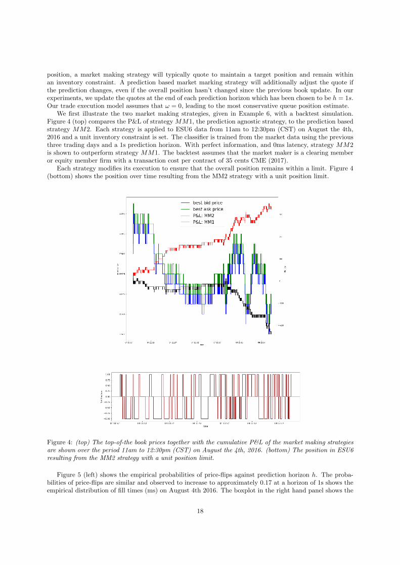
We first illustrate the two market making strategies, given in Example 6, with a backtest simulation.Figure 4 (top) compares the P&L of strategy MM1, the prediction agnostic strategy, to the prediction basedstrategy MM2. Each strategy is applied to ESU6 data from 11am to 12:30pm (CST) on August the 4th,2016 and a unit inventory constraint is set. The classifier is trained from the market data using the previousthree trading days and a 1s prediction horizon. With perfect information, and 0ms latency, strategy MM2is shown to outperform strategy MM1. The backtest assumes that the market maker is a clearing memberor equity member firm with a transaction cost per contract of 35 cents CME (2017).

Each strategy modifies its execution to ensure that the overall position remains within a limit. Figure 4(bottom) shows the position over time resulting from the MM2 strategy with a unit position limit.

Figure 4: (top) The top-of-the book prices together with the cumulative P&L of the market making strategiesare shown over the period 11am to 12:30pm (CST) on August the 4th, 2016. (bottom) The position in ESU6resulting from the MM2 strategy with a unit position limit.

Figure 5 (left) shows the empirical probabilities of price-flips against prediction horizon h. The proba-bilities of price-flips are similar and observed to increase to approximately 0.17 at a horizon of 1s shows theempirical distribution of fill times (ms) on August 4th 2016. The boxplot in the right hand panel shows the

18

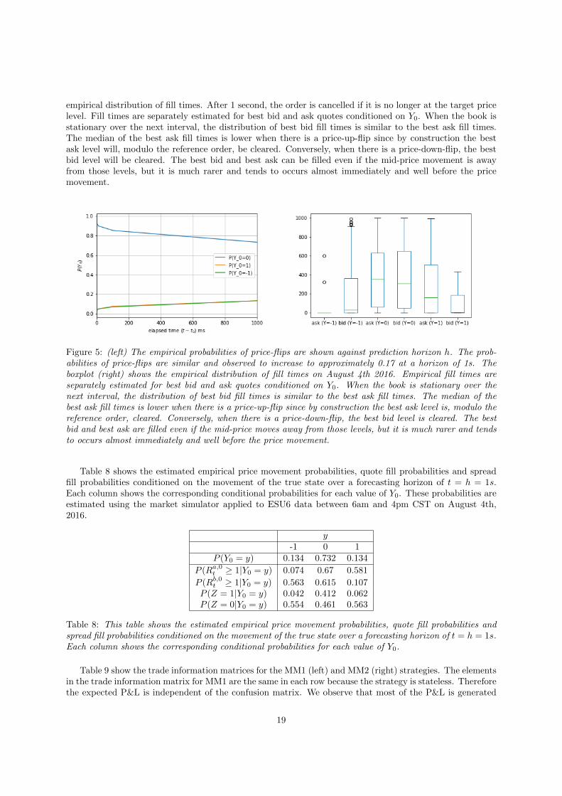
empirical distribution of fill times. After 1 second, the order is cancelled if it is no longer at the target pricelevel. Fill times are separately estimated for best bid and ask quotes conditioned on Y0. When the book isstationary over the next interval, the distribution of best bid fill times is similar to the best ask fill times.The median of the best ask fill times is lower when there is a price-up-flip since by construction the bestask level will, modulo the reference order, be cleared. Conversely, when there is a price-down-flip, the bestbid level will be cleared. The best bid and best ask can be filled even if the mid-price movement is awayfrom those levels, but it is much rarer and tends to occurs almost immediately and well before the pricemovement.

Figure 5: (left) The empirical probabilities of price-flips are shown against prediction horizon h. The prob-abilities of price-flips are similar and observed to increase to approximately 0.17 at a horizon of 1s. Theboxplot (right) shows the empirical distribution of fill times on August 4th 2016. Empirical fill times areseparately estimated for best bid and ask quotes conditioned on Y0. When the book is stationary over thenext interval, the distribution of best bid fill times is similar to the best ask fill times. The median of thebest ask fill times is lower when there is a price-up-flip since by construction the best ask level is, modulo thereference order, cleared. Conversely, when there is a price-down-flip, the best bid level is cleared. The bestbid and best ask are filled even if the mid-price moves away from those levels, but it is much rarer and tendsto occurs almost immediately and well before the price movement.

Table 8 shows the estimated empirical price movement probabilities, quote fill probabilities and spreadfill probabilities conditioned on the movement of the true state over a forecasting horizon of t = h = 1s.Each column shows the corresponding conditional probabilities for each value of Y0. These probabilities areestimated using the market simulator applied to ESU6 data between 6am and 4pm CST on August 4th,2016.

y-1 0 1

P (Y0 = y) 0.134 0.732 0.134

P (Ra,0t ≥ 1|Y0 = y) 0.074 0.67 0.581

P (Rb,0t ≥ 1|Y0 = y) 0.563 0.615 0.107P (Z = 1|Y0 = y) 0.042 0.412 0.062P (Z = 0|Y0 = y) 0.554 0.461 0.563

Table 8: This table shows the estimated empirical price movement probabilities, quote fill probabilities andspread fill probabilities conditioned on the movement of the true state over a forecasting horizon of t = h = 1s.Each column shows the corresponding conditional probabilities for each value of Y0.

Table 9 show the trade information matrices for the MM1 (left) and MM2 (right) strategies. The elementsin the trade information matrix for MM1 are the same in each row because the strategy is stateless. Thereforethe expected P&L is independent of the confusion matrix. We observe that most of the P&L is generated

19

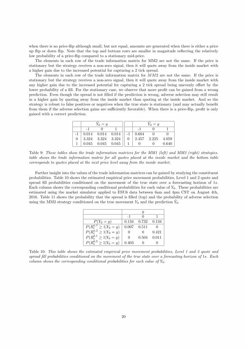
when there is no price-flip although small, but not equal, amounts are generated when there is either a priceup flip or down flip. Note that the top and bottom rows are smaller in magnitude reflecting the relativelylow probability of a price-flip compared to a stationary mid-price.

The elements in each row of the trade information matrix for MM2 are not the same. If the price isstationary but the strategy receives a non-zero signal, then it will quote away from the inside market witha higher gain due to the increased potential for capturing a 2 tick spread.

The elements in each row of the trade information matrix for MM2 are not the same. If the price isstationary but the strategy receives a non-zero signal, then it will quote away from the inside market withany higher gain due to the increased potential for capturing a 2 tick spread being unevenly offset by thelower probability of a fill. For the stationary case, we observe that more profit can be gained from a wrongprediction. Even though the spread is not filled if the prediction is wrong, adverse selection may still resultin a higher gain by quoting away from the inside market than quoting at the inside market. And so thestrategy is robust to false positives or negatives when the true state is stationary (and may actually benefitfrom them if the adverse selection gains are sufficiently favorable). When there is a price-flip, profit is onlygained with a correct prediction.

Y0 = y-1 0 1

-1 0.014 0.014 0.0140 3.324 3.324 3.3241 0.045 0.045 0.045

Y0 = y-1 0 1

-1 0.604 0 00 2.457 2.225 4.0591 0 0 0.640

Table 9: These tables show the trade information matrices for the MM1 (left) and MM2 (right) strategies.table shows the trade information matrix for all quotes placed at the inside market and the bottom tablecorresponds to quotes placed at the next price level away from the inside market.

Further insight into the values of the trade information matrices can be gained by studying the constituentprobabilities. Table 10 shows the estimated empirical price movement probabilities, Level 1 and 2 quote andspread fill probabilities conditioned on the movement of the true state over a forecasting horizon of 1s.Each column shows the corresponding conditional probabilities for each value of Y0. These probabilities areestimated using the market simulator applied to ESU6 data between 6am and 4pm CST on August 4th,2016. Table 11 shows the probability that the spread is filled (top) and the probability of adverse selectionusing the MM2 strategy conditioned on the true movement Y0 and the prediction Y0.

y-1 0 1

P (Y0 = y) 0.134 0.732 0.134

P (Ra,1t ≥ 1|Y0 = y) 0.007 0.511 0

P (Ra,2t ≥ 1|Y0 = y) 0 0 0.421

P (Rb,1t ≥ 1|Y0 = y) 0 0.504 0.011

P (Rb,2t ≥ 1|Y0 = y) 0.403 0 0

Table 10: This table shows the estimated empirical price movement probabilities, Level 1 and 2 quote andspread fill probabilities conditioned on the movement of the true state over a forecasting horizon of 1s. Eachcolumn shows the corresponding conditional probabilities for each value of Y0.

20

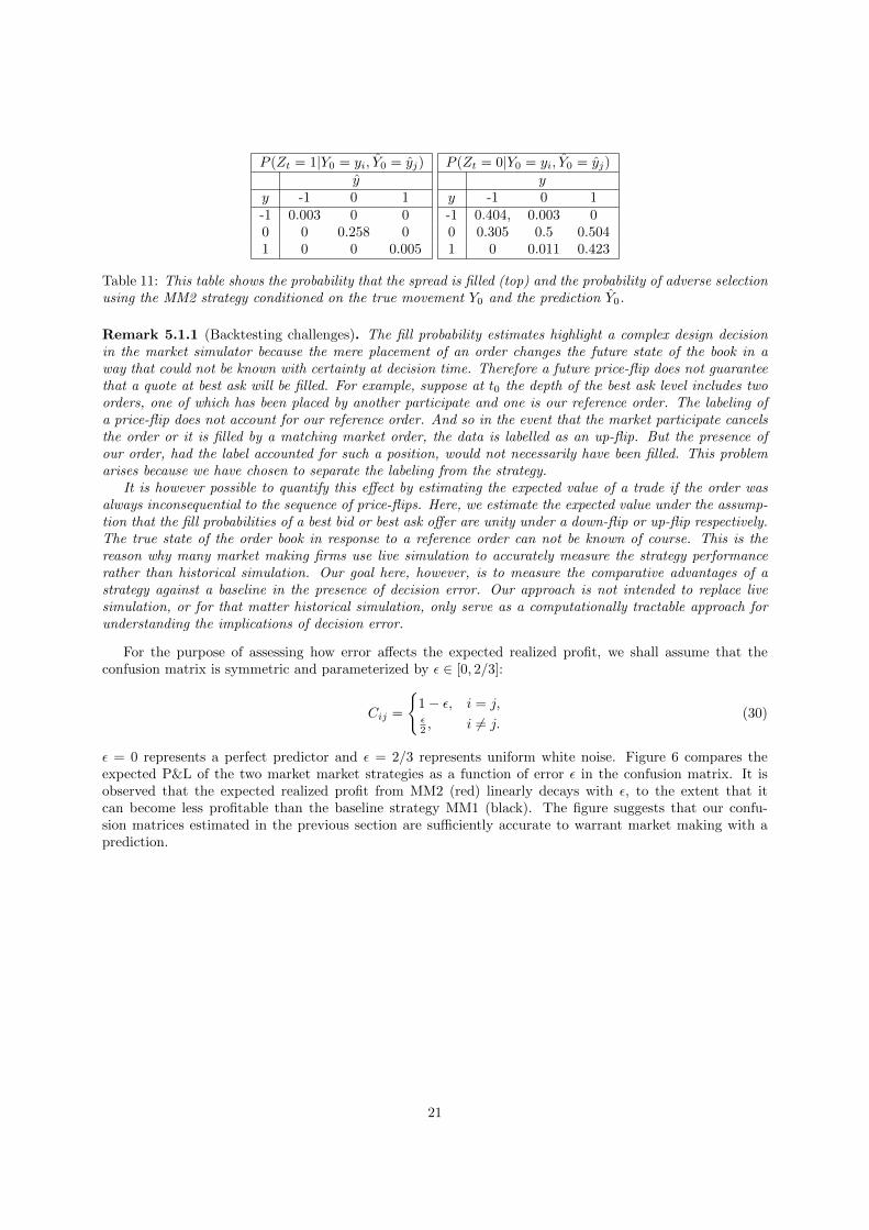
P (Zt = 1|Y0 = yi, Y0 = yj)y

y -1 0 1-1 0.003 0 00 0 0.258 01 0 0 0.005

P (Zt = 0|Y0 = yi, Y0 = yj)y

y -1 0 1-1 0.404, 0.003 00 0.305 0.5 0.5041 0 0.011 0.423

Table 11: This table shows the probability that the spread is filled (top) and the probability of adverse selectionusing the MM2 strategy conditioned on the true movement Y0 and the prediction Y0.

Remark 5.1.1 (Backtesting challenges). The fill probability estimates highlight a complex design decisionin the market simulator because the mere placement of an order changes the future state of the book in away that could not be known with certainty at decision time. Therefore a future price-flip does not guaranteethat a quote at best ask will be filled. For example, suppose at t0 the depth of the best ask level includes twoorders, one of which has been placed by another participate and one is our reference order. The labeling ofa price-flip does not account for our reference order. And so in the event that the market participate cancelsthe order or it is filled by a matching market order, the data is labelled as an up-flip. But the presence ofour order, had the label accounted for such a position, would not necessarily have been filled. This problemarises because we have chosen to separate the labeling from the strategy.

It is however possible to quantify this effect by estimating the expected value of a trade if the order wasalways inconsequential to the sequence of price-flips. Here, we estimate the expected value under the assump-tion that the fill probabilities of a best bid or best ask offer are unity under a down-flip or up-flip respectively.The true state of the order book in response to a reference order can not be known of course. This is thereason why many market making firms use live simulation to accurately measure the strategy performancerather than historical simulation. Our goal here, however, is to measure the comparative advantages of astrategy against a baseline in the presence of decision error. Our approach is not intended to replace livesimulation, or for that matter historical simulation, only serve as a computationally tractable approach forunderstanding the implications of decision error.

For the purpose of assessing how error affects the expected realized profit, we shall assume that theconfusion matrix is symmetric and parameterized by ε ∈ [0, 2/3]:

Cij =

1− ε, i = j,ε2 , i 6= j.

(30)

ε = 0 represents a perfect predictor and ε = 2/3 represents uniform white noise. Figure 6 compares theexpected P&L of the two market market strategies as a function of error ε in the confusion matrix. It isobserved that the expected realized profit from MM2 (red) linearly decays with ε, to the extent that itcan become less profitable than the baseline strategy MM1 (black). The figure suggests that our confu-sion matrices estimated in the previous section are sufficiently accurate to warrant market making with aprediction.

21

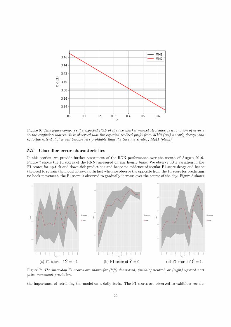
Figure 6: This figure compares the expected P&L of the two market market strategies as a function of error εin the confusion matrix. It is observed that the expected realized profit from MM2 (red) linearly decays withε, to the extent that it can become less profitable than the baseline strategy MM1 (black).

5.2 Classifier error characteristics

In this section, we provide further assessment of the RNN performance over the month of August 2016.Figure 7 shows the F1 scores of the RNN, measured on any hourly basis. We observe little variation in theF1 scores for up-tick and down-tick predictions and hence no evidence of secular F1 score decay and hencethe need to retrain the model intra-day. In fact when we observe the opposite from the F1 score for predictingno book movement- the F1 score is observed to gradually increase over the course of the day. Figure 8 shows

0.14

0.16

0.18

0.20

6−7a

m

7−8a

m

8−9a

m

9−10

am

10−

11am

11−

12pm

12−

1pm

1−2p

m

2−3p

m

3−4p

m

days

F1(

−1)

uncertainty

Median

0.6

0.7

0.8

6−7a

m

7−8a

m

8−9a

m

9−10

am

10−

11am

11−

12pm

12−

1pm

1−2p

m

2−3p

m

3−4p

m

days

F1(

0)

uncertainty

Median

0.13

0.15

0.17

0.19

0.21

6−7a

m

7−8a

m

8−9a

m

9−10

am

10−

11am

11−

12pm

12−

1pm

1−2p

m

2−3p

m

3−4p

m

days

F1(

1)

uncertainty

Median

(a) F1 score of Y = −1 (b) F1 score of Y = 0 (b) F1 score of Y = 1.

Figure 7: The intra-day F1 scores are shown for (left) downward, (middle) neutral, or (right) upward nextprice movement prediction.

the importance of retraining the model on a daily basis. The F1 scores are observed to exhibit a secular

22

decay when the model is not re-trained on a daily basis but instead trained only at the beginning of themonth. While the evidence for secular decay is clear, it is surprising to observe that a model trained at thebeginning of the month can still be effective weeks later. Typically econometrics models for non-stationarytime series perform very poorly when not frequently re-fitted to new data. This surprising model robustness,without re-training, suggests a robust relationship between the liquidity imbalance and price movements.

0.10

0.14

0.18

2016

−08

−04

2016

−08

−05

2016

−08

−08

2016

−08

−09

2016

−08

−10

2016

−08

−11

2016

−08

−12

2016

−08

−15

2016

−08

−16

2016

−08

−17

2016

−08

−18

2016

−08

−19

2016

−08

−22

2016

−08

−23

2016

−08

−24

2016

−08

−25

2016

−08

−26

2016

−08

−29

2016

−08

−30

2016

−08

−31

days

F1(

−1)

Median (with)

Median (without)

0.70

0.75

0.80

0.85

0.90

2016

−08

−04

2016

−08

−05

2016

−08

−08

2016

−08

−09

2016

−08

−10

2016

−08

−11

2016

−08

−12

2016

−08

−15

2016

−08

−16

2016

−08

−17

2016

−08

−18

2016

−08

−19

2016

−08

−22

2016

−08

−23

2016

−08

−24

2016

−08

−25

2016

−08

−26

2016

−08

−29

2016

−08

−30

2016

−08

−31

days

F1(

0) Median (with)

Median (without)

0.10

0.15

0.20

2016

−08

−04

2016

−08

−05

2016

−08

−08

2016

−08

−09

2016

−08

−10

2016

−08

−11

2016

−08

−12

2016

−08

−15

2016

−08

−16

2016

−08

−17

2016

−08

−18

2016

−08

−19

2016

−08

−22

2016

−08

−23

2016

−08

−24

2016

−08

−25

2016

−08

−26

2016

−08

−29

2016

−08

−30

2016

−08

−31

days

F1(

1) Median (with)

Median (without)

(a) F1 score of Y = −1 (b) F1 score of Y = 0 (b) F1 score of Y = 1.

Figure 8: The F1 scores over the calendar month, with (red) and without (blue) daily retraining of the RNN,are shown for (left) downward, (middle) neutral, or (right) upward next price movement prediction.

Figure 9 compares the Receiver Operator Characteristic (ROC) curves of a binary RNN classifier overvarying prediction horizons. The plot is constructed by varying the probability threshold (a.k.a. cut-points)for positive classification Y = 1 over the interval [0.5, 1) and estimating the true positive and true negativerate of each model. The dashed line shows the performance of a white-noise classifier. We observe that theperformance of the RNN decays as we increase the prediction horizon from the next book update event to 1sin the future. Latency between trading systems and the exchange is dependent on several factors includingthe execution platform, the distance of the co-located server to the exchange and even the amount of incomingtraffic to the CME matching engines. It is commonplace however for this latency to lie in the range of 100micro-seconds to 1ms. Our estimate, based on preliminary investigation, is that a c/c++ implementationof our RNN can predict in around 100 micro-seconds on a modern CPU with compiler optimizations butwithout low level programming techniques for code optimization.

23

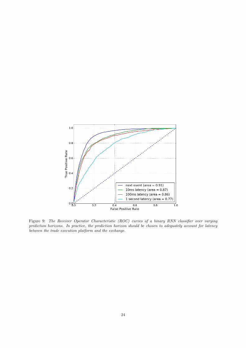
Figure 9: The Receiver Operator Characteristic (ROC) curves of a binary RNN classifier over varyingprediction horizons. In practice, the prediction horizon should be chosen to adequately account for latencybetween the trade execution platform and the exchange.

24

6 Conclusion

This paper introduces a trade execution model to evaluate the economic impact of classifiers for high fre-quency market making. We present a trade information matrix to attribute the expected profit and loss oftick level predictive classifiers. This attribution considers execution constraints such as fill probabilities andposition dependent trade rules. Our findings suggest that our approach can be a valuable and computation-ally tractable addition to standard market simulation based backtesting. In particular, it allows strategiesto be compared given the confusion matrix of the classifier and could even be used to tailor a strategy to theaccuracy characteristics of the classifier. Some of these characteristics have been presented for ESU6 overthe month of August 2016.

For machine learning and our trade information matrix to be of practical use in market making, a numberof questions remain as a corollary of this research. Some of these questions relate to the machine learningitself. For example, how can the prediction label Yt account for the impact of a trade on the state of thebook when the decision to trade is itself based on a prediction Yt of that label? Is reinforcement learning thebest approach for addressing this issue, as described for market taking in Kearns and Nevmyvaka (2013)?How much latency does a RNN model add to the quote time if implemented efficiently? Then there arequestions surrounding the trade information matrix; How frequently should the fill probability estimates beupdated? Should fill probabilities be conditioned on time of day and, perhaps, other periodic events such asearnings announcements?

Our preliminary findings suggest that there is merit in applying non-linear classifiers, such as RNNs,to Level 2 data. Instead of asking the question ’can machine learning be used for high frequency marketmaking?’, we believe that this paper advances this discussion to a question of how much error is tolerablewhen machine learning based strategies are used for avoiding adverse selection.

References

M. Abadi, P. Barham, J. Chen, Z. Chen, A. Davis, J. Dean, et al. TensorFlow: A System for Large-scaleMachine Learning. In Proceedings of the 12th USENIX Conference on Operating Systems Design andImplementation, OSDI’16, pages 265–283, 2016.

R. Bhowmik. Data mining techniques in fraud detection. Journal of Digital Forensics, Security and Law, 3,2008.

C. M. Bishop. Pattern Recognition and Machine Learning (Information Science and Statistics). Springer-Verlag New York, Inc., Secaucus, NJ, USA, 2006. ISBN 0387310738.

R. Bloomfield, M. O’Hara, and G. Saar. The ”make or take” decision in an electronic market: Evidence onthe evolution of liquidity. Journal of Financial Economics, 75(1):165–199, 2005.

L. Breiman. Statistical Modeling: The Two Cultures (with comments and a rejoinder by the author).Statistical Science, 16(3):199–231, 2001. ISSN 0883-4237, 2168-8745.

E. Budish, P. Cramton, and J. Shim. The high-frequency trading arms race: Frequent batch auctions as amarket design response. The Quarterly Journal of Economics, 130(4):1547, 2015.

C. Cao, O. Hansch, and X. Wang. The information content of an open limit order book. Journal of FuturesMarkets, 29:16–41, 2009.

J. A. Chavez-Casillas and J. E. Figueroa-Lopez. A one-level limit order book model with memory andvariable spread. Stochastic Processes and their Applications, 127(8):2447–2481, 2017.

CME. Fee summary guide: proprietary trading firms. Technical report, CME Group, January 2017. URLhttp://www.cmegroup.com/clearing/files/fee-summary-guide-for-proprietary-trading-firms.pdf.

R. Cont and A. de Larrard. Linking volatility with order flow: heavy traffic approximations anddiffusionlimits of order book dynamics. Working paper, 2010.

25

R. Cont and A. de Larrard. Price dynamics in a markovian limit order market. SIAM Journal on FinancialMathematics, 4(1):1–25, 2013. doi: 10.1137/110856605. URL https://doi.org/10.1137/110856605.

R. Cont, S. Stoikov, and R. Talreja. A stochastic model for order book dynamics. Operations Research, 58:549–563, 2010a.

R. Cont, S. Stoikov, and R. Talreja. A stochastic model for order book dynamics. Operations Research, 58(3):549–563, 2010b. ISSN 0030364X, 15265463. URL http://www.jstor.org/stable/40792679.

R. Cont, S. Kukanov, and S. Stoikov. The price impact of order book events. Journal of Financial Econo-metrics, 12:47–88, 2014.

M. Dixon. Sequence classification of the limit order book using recurrent neural networks. Journal ofComputational Science, 2017. ISSN 1877-7503. doi: https://doi.org/10.1016/j.jocs.2017.08.018. URLhttp://www.sciencedirect.com/science/article/pii/S1877750317309675.

M. Dixon, D. Klabjan, and J. H. Bang. Classification-based financial markets prediction using deep neuralnetworks. Algorithmic Finance, 2016.

M. Dixon, N. Polson, and V. Sokolov. Deep learning for spatio-temporal modeling: Dynamic traffic flowsand high frequency trading. arXiv preprint arXiv:1705.09851, 2017.

D. Dobrislav and E. Schaumburg. High-frequency cross-market trading: Model free measurement and ap-plications. Technical report, Federal Reserve Bank of New York, 2016.

R. F. Engle and J. R. Russell. Autoregressive conditional duration: A new model for irregularlyspaced transaction data. Econometrica, 66(5):1127–1162, 1998. ISSN 00129682, 14680262. URLhttp://www.jstor.org/stable/2999632.

J. Farmer and S. Spyros. Review of the benefits of a continuous market vs. randomised stop auctions and ofalternative priority rules (policy options 7 and 12). Technical report, UK Government Office for Science,2012.

J. Friedman, T. Hastie, and R. Tibshirani. Regularization paths for generalized linear models via coordinatedescent. Journal of Statistical Software, 33(1):1–22, 2010.

X. Glorot and Y. Bengio. Understanding the difficulty of training deep feedforward neural networks. InIn Proceedings of the International Conference on Artificial Intelligence and Statistics (AISTATS?10).Society for Artificial Intelligence and Statistics, 2010.

L. Glosten. Is the electronic open limit order book inevitable? Journal of Finance, pages 1127–1161, 1994.

A. Graves. Generating sequences with recurrent neural networks. CoRR, abs/1308.0850, 2013. URLhttp://arxiv.org/abs/1308.0850.

T. Hastie, R. Tibshirani, and J. Friedman. The Elements of Statistical Learning. Springer Series in Statistics.Springer New York Inc., New York, NY, USA, 2001.

T. Hendershott, C. M. Jones, and A. J. Menkveld. Does algorithmic trading improve liquidity? The Journalof Finance, 66(1):1–33, 2011. ISSN 1540-6261.

M. Kearns and Y. Nevmyvaka. Machine learning for market microstructure and high frequency trading.High Frequency Trading - New Realities for Traders, 2013.

A. Kercheval and Y. Zhang. Modeling high-frequency limit order book dynamics with support vector ma-chines. Journal of Quantitative Finance, 15(8):1315–1329, 2015.

R. Kozhan and M. Salmon. The information content of a limit order book:the case of an FX market. Journalof Financial Markets, 15, 2012.

26

M. Leung, H. Daouk, and A. Chen. Forecasting stock indices: A comparison of classification and levelestimation models. International Journal of Forecasting, 16(2):173–190, 2000.

D. Palguna and I. Pollak. Mid-price prediction in a limit order book. IEEE Journal of Selected Topics inSignal Processing, 10, 2014.

C. Parlour. Price dynamics in limit order markets,. Review of Financial Studies, 11:789–816, 1998.

R. Rojas. Neural Networks: A Systematic Introduction. Springer-Verlag New York, Inc., New York, NY,USA, 1996. ISBN 3-540-60505-3.

D. Seppi. Liquidity provision with limit orders and strategic specialist. The Review of Financial Studies, 10(1):103–150, 1997.

N. Simon, J. Friedman, T. Hastie, and R. Tibshirani. Regularization Paths for Cox’s Proportional HazardsModel via Coordinate Descent. Journal of Statistical Software, 39(5):1–13, 2011.

J. A. Sirignano. Deep learning for limit order books. arXiv preprint arXiv:1601.01987, 2016.

N. Srivastava, G. E. Hinton, A. Krizhevsky, I. Sutskever, and R. Salakhutdinov. Dropout: a simple way toprevent neural networks from overfitting. Journal of Machine Learning Research, 15(1):1929–1958, 2014.

B. Zheng, E. Moulines, and F. Abergel. Price jump prediction in a limit order book. Journal of MathematicalFinance, 3:242–255, 2013.

27