High Frequency (HF) radio signal amplitude characteristics

Calhoun: The NPS Institutional Archive

Theses and Dissertations Thesis Collection

1990-06

High Frequency (HF) radio signal amplitude

characteristics, HF receiver site performance criteria,

and expanding the dynamic range of HF digital new

energy receivers by strong signal elimination

Lott, Gus K., Jr.

Monterey, California: Naval Postgraduate School

http://hdl.handle.net/10945/34806

NPS62-90-006

NAVAL POSTGRADUATE SCHOOL Monterey, ,California

DISSERTATION

HIGH FREQUENCY (HF) RADIO SIGNAL AMPLITUDE CHARACTERISTICS, HF RECEIVER SITE PERFORMANCE CRITERIA, and

EXPANDING THE DYNAMIC RANGE OF HF DIGITAL NEW ENERGY RECEIVERS BY STRONG SIGNAL ELIMINATION

by

Gus K. lott, Jr.

June 1990

Dissertation Supervisor: Stephen Jauregui

!)1!tmlmtmOlt tlMm!rJ to tJ.s. eave"ilIE'il Jlcg6iielw olil, 10 piolecl ailicallecl",olog't dU'ie 18S8. Btl,s, refttteste fer litis dOCdiii6i,1 i'lust be ,ele"ed to Sapeihil6iiddiil, 80de «Me, "aial Postg;aduulG Sclleel, MOli'CIG" S,e, 98918 &988 SF 8o'iUiid'ids" PM::; 'zt6lI44,Spawd"d t4aoal \\'&u 'al a a,Sloi,1S eai"i,al'~. 'Nsslal.;gtePl. Be 29S&B &198 .isthe 9aleMBe leclu,sicaf ,.,FO'iciaKe" 6alite., ea,.idiO'. Statio", AlexB •• d.is, VA. !!!eN 8'4!.

,;M.41148 'fl'is dUcO,.Mill W'ilai.,s aliilical data wlrose expo,l is idst,icted by tli6 Arlil! Eurse" SSPItial "at FRIis ee, 1:I.9.e. gec. ii'S1 sl. seq.) 01 tlls Exr;01l ftle!lIi"isllatioli Act 0' 19i'9, as 1tI'I'I0"e!ee!, "Filill ell, W.S.€'I ,0,,,,, 1i!4Q1, III: IIlIiI. 'o'iolatioils of ltrese expo,lla;;s ale subject to 960616 an.iudl pSiiaities. Bissaiiiiiaia iii acco.dullcG "UIi J:SlooisiclI3 of Ofl'4AVIl4Me518.18I, ,eleloliee tii.).

BESfRtIefI6ff .fefieE Basbo, b, all, mailloe! Ihal niH plaisllt e!iseloslua II' OOlltellte IIf i'ellelletAlelie,. ef tAli e!e elf""e,.,. .

Prepared for: Commander (PMW-143/144) Space and Naval Warfare Systems Command Washington, DC 200~-5100

Commander (G80/43) Naval Securlty Group Command 3801 Nebraska Ave. Washington, DC 20393-5213

Approved for public release; distribution is unlimited

THIS PAGE INTENTIONALLY LEFT BLANK

h t t p : / / w w w . n p s . e d u

DUDLEY KNOX LIBRARY.

January 20, 2011 SUBJECT: Change in distribution statement for High Frequency (HF) Radio Signal Amplitude Characteristics, HF receiver Site Performance Criteria, and Expanding the Dynamic Range of HF Digital New Energy Receivers by Strong Signal Elimination – June 1990. 1. Reference: Lott, Gus K., Jr. High Frequency (HF) Radio Signal Amplitude Characteristics, HF

receiver Site Performance Criteria, and Expanding the Dynamic Range of HF Digital New Energy Receivers by Strong Signal Elimination. Monterey, CA: Naval Postgraduate School, June 1990. UNCLASSIFIED [Distribution authorized to US. Government Agencies only; Critical Technology; June 1990].

2. Upon consultation with NPS faculty, the School has determined that this thesis may be released to

the public and that its distribution is unlimited, effective December 16, 2010.

University Librarian Naval Postgraduate School

THIS PAGE INTENTIONALLY LEFT BLANK

UNCLASSIFIED SF CATION OF THIS PAGE SECURITY CLAS I I

Form Approved REPORT DOCUMENTATION PAGE OMBNo.0704-0188

la. REPORT SECURITY CLASSIFICATION 1 b. RESTRICTIVE MARKINGS UNCLASSIFIED

2a. SECURITY CLASSIFICATION AUTHORITY 3. DISTRIBUTION I AVAILABILITY OF REPORT BistributiOfi limited to H.S. Eiouernment

2b. DECLASSIFICATION I DOWNGRADING SCHEDULE (l!;ene!te~ oftl, te p!!'e~eet e'l!'~t~ee~ teeftfte , ¥ , nnn r. ~~ ~

4. PERFORMING ORGANIZATION REPORT NUMBER{S) S. MONITORING ORGANIZATION REPORT NUMBER{S)

NPS62-90-006 . 6a. NAME OF PERFORMING ORGANIZATION 6b. OFFICE SYMBOL 7a. NAME OF MONITORING ORGANIZATION

(If applicable)

Naval Postgraduate School EC Naval Postgraduate School 6c. ADDRESS (City, State, and ZIP Code) 7b. ADDRESS (City, State, and ZIP Code)

Monterey, CA 93943-S100 Monterey, CA 93943-S100

Ba. NAME OF FUNDING ISPONSORING 8b. OFFICE SYM80L 9. PROCUREMENT INSTRUMENT IDENTifiCATION NUMBER ORGANIZATION (If applicable) SPACETASKS 143-1-89-4SBM-00S and Space and Naval Warfare

PMW 143/144 144-2-89-PGS-4SBN-03S Svstems Command Be. ADDRESS (City, State, and ZIP Code) 10. SOURCE OF FUNDING NUMBERS Commander (PMW-143/144) PROGRAM PROJECT TASK WORK UNIT Space and Naval Warfare Systems Command ELEMENT NO. NO. NO. ACCESSION NO.

Washington DC 20363 S100 11. TITLE (Include Security Classification)

HIGH FREQUENCY (HF) RADIO SIGNAL AMPLITUDE CHARACTERISTICS, HF RECEIVER SITE PERFORMANCE, and EXPANDING THE DYNAMIC RANGE OF HF DIGITAL NEW ENRRr.V RFr.P,TVP,RS RV S'1'RONr. <::TCNAT

12. PERSONAL AUTHOR{S) Lott, Gus K.

13a. TYPE OF REPORT J13b TIME COVERED Doctoral Dissertation FROM TO

r4 . DATE OF REPORT (Year, Month, Day) r 5. PAGE COUNT 1990, June, 21 2S7

16. SUPPLEMENTARY NOTATION The views expressed in this dissertation are those of the author and do not reflect the official policy or position of the Department of Defense or the U.S Go ~nt-

17. COSA TI CODES 18. SUBJECT TERMS (Continue on reverse if necessary and identify by block number)

FIELD GROUP SUB-GROUP HF Signals; HF Receiver; Wideband Receiver; Spectrum Survey; HF Signal Amplitude Probability Distribution; Log· normal· Receiver Si rp pprfnrm~n('p· ;:m~l no--rr.-A; n; 1-",1

19. ABSTRACT (Continue on reverse if necessary and identify by block number)

The dissertation discusses High Frequency (HF) radio sources. It consolidates data from all available, published HF spectrum surveys. The author conducted a new HF survey using detection of new energy events. The first cumulative probability dist~ibution function for the amplitude of detected non-broadcast HF signals is developed, and the distribution is log-normal. HF receiver site performance quantification is possible using the HF signal distributions. Site performance degredation results from noise, interference, and signal path attenuation. Noise examples are presented in a 3-D format of time, frequency, and amplitude. Graphs are presented that allow estimation of the percentage of HF non-broadcast signals lost as a function of noise and interferece levels. Limitations of HF search receivers using analog-to-digital converters as the receiver front-end are discussed. Derived bounds on A/D converter performance show that today's digital technology does not provide enough dynamic range, sensitivity, or

20. DISTRIBUTION I AVAILABILITY OF ABSTRACT 21. ABSTRACT SECURITY CLASSIFICATION KlUNCLASSIFIED/UNLIMITED o SAME AS RPT. o DTIC USERS UNCLASSIFIED

22a. NAME OF RESPONSIBLE INDIVIDUAL Stephen Jauregui

DO Form 1473, JUN 86

22b. TELEPHONE (Include Area Code) 122c. OFFICE SYMBOL (408) 646-2753 EC/Ja

Previous editions are obsolete.

SiN 0102-LF-014-6603 i

SECURITY CLASSIFICATION OF THIS PAGE UNCLASSIFIED

UNCLASSIFIED SECURITY CLASSIFICATION OF THIS PAGE

3. continued

docah,cnl! mas t be i cEeL t cd to Saper intcneicnt, SeaL 943, liao a1 Pos t!)raauatoe Selteel, HOllcerey, e* "3"43 seee or eOlllli£andcr, P?Hl llf3/144 , St'aee efta Ne hal l1a!'fe!'e gyS~9111:S Connnaild, WasirlngL,on, Be 28363 5188 via LIIE Befense 'fecliiiical InfoifitaLioii SeIzter, eamEIOiI Station, Alexandria, VA 22394 6145.

liar ding 'Iris dOCUilrEnL contains tecilliical data wllose expol L . is i es tr ie ted b, tIle *rms Export Control *ct (titlE 22, 8.S.e. Sec. 2751 ct. eet):.) er the :S'[IHH~t: Administration Act of 1~7~, as annuEllded, 'fiLlt 59,"'8.8.0., i\~l' 2 l,Ql, eel eeEfu T.TielaLions of tltEsE export lawS are subject to SEVErE criminal penalties. BisseurinaLe tn accordancE wiLlI pruiisiotLs of OPIW/IliS'f 5518.161, refereftee (jj.).

Approved for public release; distribution is unlimited 11. continued

ELIMINATION

18. continued

converter; AID; Electromagneticcompatability; dynamic range; new energy detection; strong signal elimination

19. continued

sampling rate. Alternative dynamic range extension methods are examined. A new method of dynamic range extension by removing the strongest signals present is presented. Greater receiver sensitivity results from changing the HF signal environment seen by the AID converter. The new method uses a phase-tracking network and signal reconstruction techniques.

DO Form 1473, JUN 86 (Reverse)

ii

SECURITY CLASSIFICAT ION OF T HIS PAGE

UNCLASSIFIED

Approved for public release; distribution is unlimited

BIEffftlBI:fRet41:1MREB to 1::1.9. 80;eiiIi ilellt Agwcies 0111, to !'.otect etitlOf\J teChllOlo~" "111101999. 9th8r r8E1118ete fsr this IIIs8III'I'Ioftt I'I'IlIet 80 ,efel'l'8l11.1 Slll!oI'iMelllllo .... 91111e 948. tla ... aI Pe8t!ralllllate iSReal; USRteray, ~o QiQ4i &000 QF 9111.'111:111110'. PM'll 119/~ H.S"alo alllll tJ81al'Narflll8 S~etelll8 9sI'I'II'I'Ialllll. '}:leehiR.sR. Q9 sea8i i~99 uiatRQ gQfQRIi'Q "Feehllical "'",PI! ,Me II 90llto,. 9at 1101'81. Static I'. ;\leMallllll.ia.VA ~9 1 8116.

WMI4.,.8 "Ids dUCO"E'il wi,laiiis teeli,licaf data allOsa 8xpell is lesbicl9d bj tlie Ai,,1S &1'0,1 8s.lftel hJt fAits ee, tles.e. 3uc. 2'01 ell seq.) 0' lite ExpOit JltdiiHiiisbalioii Act of Is,a, as WiiGiided, litle 58, \!J.S.S., ""IS 2481, at. se~. Violatiolls of these el(I'0I'f: lails atC slIbject to !ecele cliliMliai I'Cllaities. BisscII.illato ill 8111,lIIa1'l18 "it" j!lI'8Yi8isRS sf 9PtlAVltlSHj619 ... 81. ref8r81'188 iji.).

HIGH FREQUENCY (HF) RADIO SIGNAL AMPLITUDE CHRARCTERISTICS, HF RECEIVER SITE PERFORMANCE CRITERIA, and

EXPANDING THE DYNAMIC RANGE OF HF DIGITAL NEW ENERGY RECEIVERS BY STRONG SIGNAL EUMINATION

by

Gus K. Lott, Jr. Lieutenant Commander. United States Navy

B.E.E .• Auburn University, 1976 M.B.A.. Corpus Christi State University, 1979

M.S .• Naval Postgraduate School. 1988

Submitted in partial fulfillment of the requirements for the degree of

DOCTOR OF PHILOSOPHY IN ELECTRICAL ENGINEERING

from the

NAVAL POSTGRADUATE SCHOOL June 1990

Author' ___________________________________________________________ ___

Approved by:

Glen A. Myers Associate Professor of

ElectFical and Comguter Engineering

Hal M. Fredricksen Department Chairman and Professor of Mathematics

Stephen Jauregui Adjunct Professor of

Electrical and Computer Engineering Dissertatic.vl SUDervisor

Gus K. Lott, Jr.

Paul H. Moose Associate Professor of

Electrical and Computer Engineering

Michael J. Zyda Associate Professor of

Computer Science

Approved by: __________________________________________________ _

John P. Powers, Chairman. Department of Electrical and Computer Engineering

Approved by: _______________ - __________ _

Harrison Shull. ProvostjAcademic Dean

iii

ABSTRACT

The dissertation discusses High Frequency (HF) radio sources. It consolidates

data from all available, published HF spectrum surveys. The author conducted a

new HF survey using detection of new energy events. The first cumulative

probability distribution function for the amplitude of detected non-broadcast HF

signals is developed, and the distribution is log-normal. HF receiver site

performance quantification is possible using the HF signal distributions. Site

performance degradation results from noise, interference, and signal path

attenuation. Noise examples are presented in a 3-D format of time, frequency, and

amplitude. Graphs are presented that allow estimation of the percentage of HF

non-broadcast signals lost as a function of noise and interference levels. Limitations

of HF search receivers using analog-to-digital converters as the receiver front-end

are discussed. Derived bounds on ND converter performance show that today's

digital technology does not provide enough dynamic range, sensitivity, or sampling

rate. Alternative dynamic range extension methods are examined. A new method

of dynamic range extension by removing the strongest signals present is presented.

Greater receiver sensitivity results from changing the HF signal environment seen

by the ND converter. The new method uses a phase-tracking network and signal

reconstruction techniques.

IV

I>.::: > ':"-:;i'-:"::. "":~:::·:.~~o;~ I:I;~.I:Z..f!.r?JY

_: .:: : ./', .. } ."i:-':);~: J .... :. ·i':,.~·~ .. I~;~:(f\.'=:T} SeEOO]".., ]l(OlijTjjJ,}~/~j'i , UiiL~U:,'OIGIT i])" f:/38!13-tJOOa

TABLE OF CONTENTS

I. INTRODUCTION ......................................................................................... 1

II. HIGH FREQUENCY ENVIRONMENT................................................ 5

A. STRONGEST SIGNAlS.................................................................... 8

B. MINIMUM-DETECTABLE SIGNAlS.......................................... 17

C. OVERALL HF DYNAMIC RANGE REQUIREMENTS........ 25

III. HF SIGNAL AMPLITUDE STATISTICS .............................................. 28

A. HF SIGNAL STUDIES...................................................................... 29

B. THE LOG-NORMAL DISTRIBUTION........................................ 36

C. ESTIMATING MEAN AND VARIANCE................................... 41

D. MATCHED LOG-NORMAL DISTRIBUTIONS ........................ 44

IV. HF NEW-ENERGY OBSERVATIONS.................................................. 46

A. EXAMPLES OF NEW ENERGIES REQUIRING.................... 49 SEARCH SCREENING

B. HF NEW-ENERGY SURVEy........................................................ 58

C. SUMMARY OF RESULTS.............................................................. 70

V. HF SITE PERFORMANCE CRITERIA................................................ 73

A. PERFORMANCE CURVES ............................................................ 75

v

B. ESTIMATING PERFORMANCE FROM SITE ......................... 79 MEASUREMENTS

C. GRAPHICAL SITE PERFORMANCE ESTIMATION ............ 91

D. DISCUSSION........................................................................................ 96

VI. NO SELECTION AND PERFORMANCE ........................................... 97

A. GENERAL NO REQUIREMENTS.............................................. 100

B. NO PERFORMANCE LIMITATIONS ........................................ 103

C. COMBINED EFFECTS ON NO DYNAMIC RANGE ........... 127

VII. NO DYNAMIC RANGE EXTENSION METHODS ......................... 130

A. GAIN-ADJUSTING AND FLOATING-POINT .......................... 131 CONVERSION

B. NONLINEAR QUANTIZATION .................................................... 134

C. OVERSAMPLING ............................................................................... 138

D. POST-CONVERSION PROCESSING ............................................ 140

E. OTHER TECHNIQUES .................................................................... 142

F. SUMMARy ........................................................................................... 143

VIII. STRONG SIGNAL ELIMINATION ......................................................... 145

A. FREQUENCY COVERAGE PLAN AND ................................... 148 NOTCH FILTERING

B. STRONG SIGNAL ELIMINATION SySTEM ............................ 151

C. MULTIPLE-STAGE STRONG SIGNAL ELIMINATION ....... 166

IX. CONCLUSIONS AND RECOMMENDATIONS .................................. 168

APPENDIX A .................................................................................................................. 172

VI

APPENDIX B .................................................................................................................. 179

APPENDIX C .................................................................................................................. 210

APPENDIX D .................................................................................................................. 215

LIST OF REFERENCES.............................................................................................. 222

BIBLIOGRAPHy............................................................................................................ 232

INITIAL DISTRIBUTION LIST ................................................................................. 235 .

VB

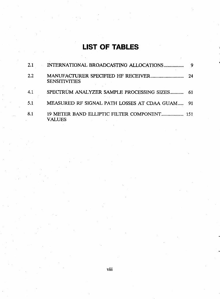
LIST OF TABLES

2.1 INTERNATIONAL BROADCASTING ALLOCATIONS.................. 9

2.2 MANUFACTURER SPECIFIED HF RECEIVER .............................. 24 SENSITIVITIES

4.1 SPECTRUM ANALYZER SAMPLE PROCESSING SIZES ............ 61

5.1 MEASURED RF SIGNAL PATH LOSSES AT CDAA GUAM..... 91

8.1 19 METER BAND ELLIPTIC FILTER COMPONENT .................... 151 VALUES

Vlll

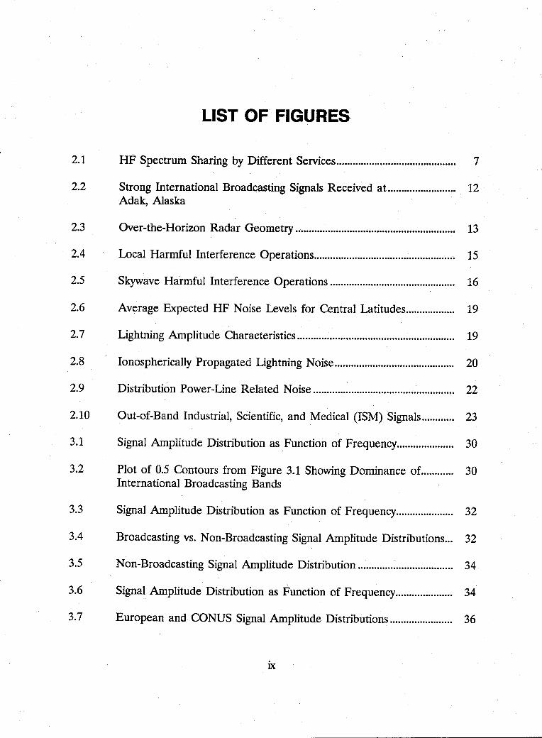
LIST OF FIGURES

2.1 HF Spectrum Sharing by Different Services............................................ 7

2.2 Strong International Broadcasting Signals Received at ......................... 12 Adak, Alaska

2.3 Over-the-Horizon Radar Geometry ........................................................... 13

2.4 Local Harmful Interference Operations.................................................... 15

2.5 Skywave Harmful Interference Operations .............................................. 16

2.6 Average Expected HF Noise Levels for Central Latitudes.................. 19

2.7 Lightning Amplitude Characteristics .......................................................... 19

2.8 Ionospherically Propagated Lightning Noise............................................ 20

2.9 Distribution Power-Line Related Noise .................................................... 22

2.10 Out-of-Band Industrial, Scientific, and Medical (ISM) Signals............ 23

3.1 Signal Amplitude Distribution as Function of Frequency..................... 30

3.2 Plot of 0.5 Contours from Figure 3.1 Showing Dominance of............ 30 International Broadcasting Bands


3.4 Broadcasting vs. Non-Broadcasting Signal Amplitude Distributions... 32

3.5 Non-Broadcasting Signal Amplitude Distribution ................................... 34


3.7 European and CONUS Signal Amplitude Distributions ....................... 36

IX

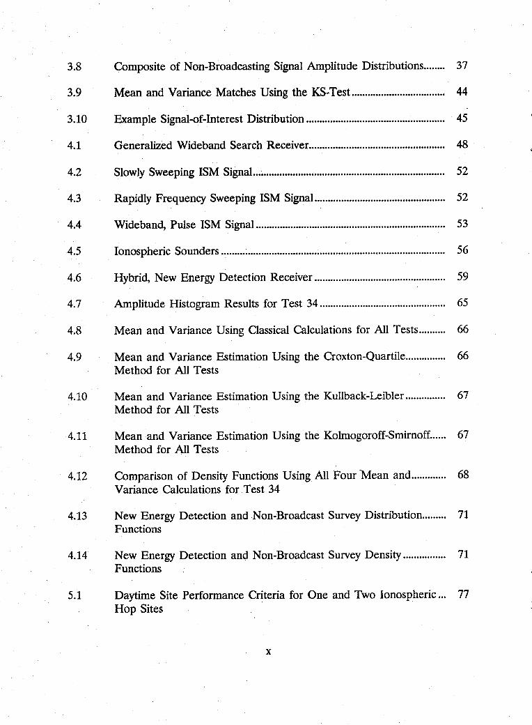
3.8 Composite of Non-Broadcasting Signal Amplitude Distributions........ 37

3.9 Mean and Variance Matches Using the KS-Test................................... 44

3.10 Example Signal-of-Interest Distribution .................................................... 45

4.1 Generalized Wideband Search Receiver................................................... 48

4.2 Slowly Sweeping ISM Signal........................................................................ 52

4.3 Rapidly Frequency Sweeping ISM Signal................................................. 52

4.4 Wideband, Pulse ISM Signal....................................................................... 53

4.5 Ionospheric Sounders .................................................................................... 56

4.6 Hybrid, New Energy Detection Receiver ................................................. 59

4.7 Amplitude Histogram Results for Test 34............................................... 65

4.8 Mean and Variance Using Classical Calculations for All Tests.......... 66

4.9 Mean and Variance Estimation Using the Croxton-Quartile............... 66 Method for All Tests

4.10 Mean and Variance Estimation Using the Kullback-Leibler ............... 67 Method for All Tests

4.11 Mean and Variance Estimation Using the Kolmogoroff-Smirnoff.. .... 67 Method for All Tests

4.12 Comparison of Density Functions Using All Four -Mean and ............. 68 Variance Calculations for Test 34

4.13 New Energy Detection and Non-Broadcast Survey Distribution ......... 71 Functions

4.14 New Energy Detection and Non-Broadcast Survey Density ................ 71 Functions

5.1 Daytime Site Performance Criteria for One and Two Ionospheric ... 77 Hop Sites

x

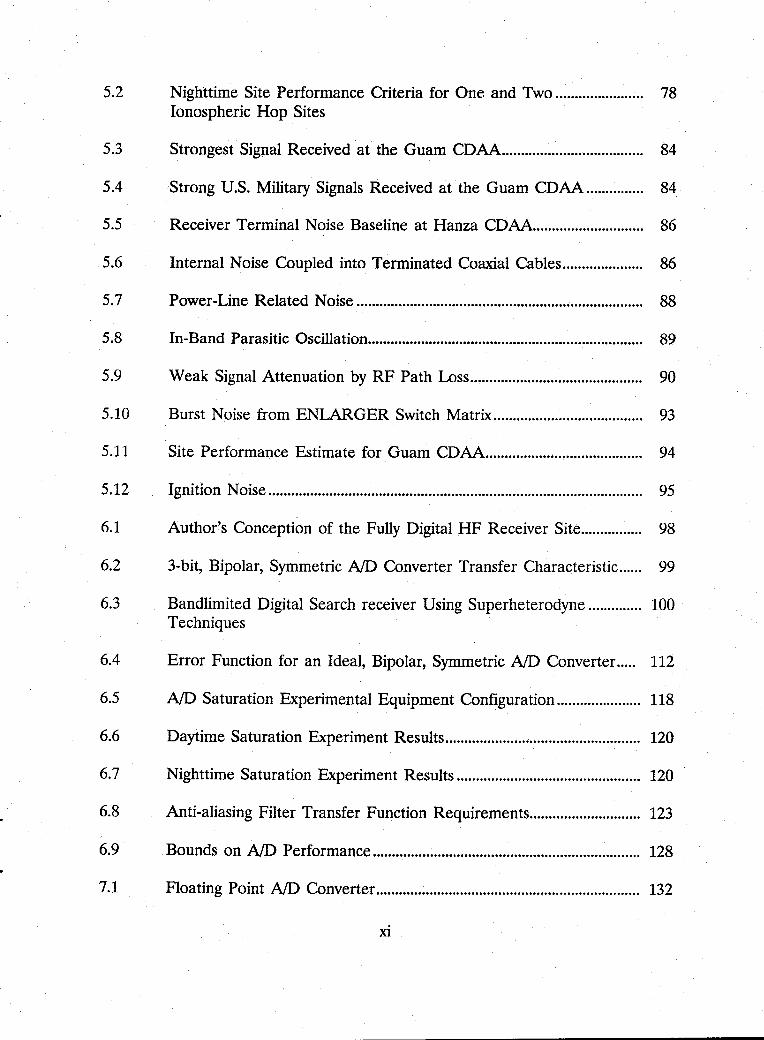
5.2 Nighttime Site Performance Criteria for One and Two ....................... 78 Ionospheric Hop Sites

5.3 Strongest Signal Received at the Guam CDAA..................................... 84

5.4 Strong U.S. Military Signals Received at the Guam CDAA ............... 84

5.5 Receiver Terminal Noise Baseline at Hanza CDAA............................. 86

5.6 Internal Noise Coupled into Terminated Coaxial Cables..................... 86

5.7 Power-Line Related Noise ........................................................................... 88

5.8 In-Band Parasitic Oscillation........................................................................ 89

5.9 Weak Signal Attenuation by RF Path Loss............................................. 90

5.10 Burst Noise from ENLARGER Switch Matrix....................................... 93

5.11 Site Performance Estimate for Guam CDAA......................................... 94

5.12 Ignition Noise.................................................................................................. 95

6.1 Author's Conception of the Fully Digital HF Receiver Site................ 98

6.2 3-bit, Bipolar, Symmetric NO Converter Transfer Characteristic...... 99

6.3 Bandlimited Digital Search receiver Using Superheterodyne .............. 100 Techniques

6.4 Error Function for an Ideal, Bipolar, Symmetric NO Converter..... 112

6.5 NO Saturation Experimental Equipment Configuration ...................... 118

6.6 Daytime Saturation Experiment Results................................................... 120

6.7 Nighttime Saturation Experiment Results ................................................ 120

6.8 Anti-aliasing Filter Transfer Function Requirements............................. 123

6.9 Bounds on NO Performance ...................................................................... 128

7.1 Floating Point NO Converter ..................................................................... 132

Xl

7.2 Parallel-Scaled NO Converter .................................................................... 134

7.3 Dynamic Range Gain by Oversampling ........................ ; ........................... 139

8.1 Strong Daytime International Broadcast Signals ..................................... 147

8.2 Strong Nighttime International Broadcast Signals .................................. 147

8.3 Receiver Coverage to Minimize International Broadcast.. ................... 149 Overloading

8.4 19 Meter Band Elliptic Notch Filter ......................................................... 150

8.5 Ideal Signal Subtraction System.................................................................. 152

8.6 RMS of Envelope Error Factor versus Peak Amplitude Difference. 160

8.7 RMS Residual Values versus Peak Amplitude Difference ................... 162

8.8 Instantaneous Residual Value ..................................................................... 162

8.9 Block Diagram of Basic Strong Signal Elimination System .................. 163

8.10 Superheterodyne Strong Signal Eliminator. .............................................. 165

8.11 Multiple Stage Strong Signal Elimination Architecture ......................... 167

A.l Block Diagram of Equipment Used to Make Noise and ..................... 172 Interference Measurements

A.2 Units of Measure Associated with Each Axis in Photographs ............ 174 Made with the 3-Axis Display System

A.3 Combined Operation of HP141T and Develco 7200 Showing ............ 175 FIFO Movement of Spectrum Analyzer Scans

A.4 Example of 3-Axis Display of HF Signals ................................................ 177

B.1 Histogram for Data Set 1, 11 April 89, 1342-1415, CF=14750 .......... 180 kHz, AT=16 dB, ADT=8 dB, b=14


XlI

B.3 Histogram for Data Set 4, 11 April 89, 1727-1957, CF=13750 .......... 181 kHz, AT=12 dB, ADT=8 dB,b=14

B.4 Histogram for Data Set 5, 11 April 89, 2006-2123, CF=5250 ............ 181 kHz, AT=25 dB, ADT=8 dB, b=14

B.5 Histogram for Data Set 6, 11-12 April 89, 2126-0527, CF=4500 ....... 182 kHz, AT=25 dB, ADT=8 dB, b=14


B.7 Histogram for Data Set 8, 19 April 89, 1209-1224, CF=13750 .......... 183 kHz, AT=O dB, ADT=8 dB, b=14

B.8 Histogram for Data Set 8, 19 April 89, 1209-1224, CF=13750 .......... 183 kHz, AT=O dB, ADT=8 dB, b=12


B.lO Histogram for Data Set 9, 19 April 89, 1225-1241, CF=13750 .......... 184 kHz, AT=4 dB, ADT=8 dB, b=12

B.ll Histogram for Data Set 11, 19 April 89, 1301-1319, CF=13750 ........ 185 kHz, AT=12 dB, ADT=8 dB, b=14

B.12 Histogram for Data Set 11, 19 April 89, 1301-1319, CF=13750 ........ 185 kHz, AT=12 dB, ADT=8 dB, b=12





xiii

. .,,'"



R19 Histogram for Data Set 15, 19 April 89, 1409-1424, CF=13750 ........ 189 kHz, AT=28 dB, ADT=8 dB, b=14










B.29 Histogram for Data Set 20, 19 April 89, 2040-2055, CF=4500 .......... 194 kHz, AT=63 dB,ADT=8 dB, b=14


xiv










BAO Histogram for Data Set 25, 19 April 89, 2158-2213, CF=4500 .......... 199 kHz, AT=40 dB, ADT=8 dB, b=12

BA1 Histogram for Data Set 26, 19 April 89, 2213-2228, CF=4500 .......... 200 kHz, AT=36 dB, ADT=8 dB, b=14

BA2 Histogram for Data Set 26, 19 April 89, 2213-2228, CF=4500 .......... 200 kHz, AT=36 dB, ADT=8 dB, b=12

BA3 Histogram for Data Set 30, 22 April 89, 1136-1253, CF=14750 ........ 201 kHz, AT=12 dB, ADT=8 dB, b=14

BA4 Histogram for Data Set 31, 22 April 89, 1259-1344, CF=13750 ........ 201 kHz, AT=12.dB, ADT=8 dB, b=14

xv





B.49 Histogram for Data Set 34, 22-23 April 89, 1524-0559, CF=7750 .... 204 kHz, AT=12 dB, ADT=16 dB, b=14

B.50 Histogram for Data Set 34, 22-23 April 89, 1524-0559, CF=7750 .... 204 kHz, AT=12 dB, ADT=8 dB, b=14

B.51 Surface Plot of Histograms for Data Sets 8-18, 19 Apr 89, ................ 205 CF=13750 kHz, AT=see plot, ADT=8 dB, b=14

B.52 Contour Plot of Histograms for Data Sets 8-18, 19 Apr 89, ............... 205 CF=13750 kHz, AT=see plot, ADT=8 dB, b=14, Contour Levels = 50 NEAs

B.53 Surface Plot of Histograms for Data Sets 8-18, 19 Apr 89, ................ 206 CF=13750 kHz, AT=see plot, ADT=8 dB, b=12

B.54 Contour Plot of Histograms for Data Sets 8-18, 19 Apr 89, ............... 206 CF=13750 kHz, AT=see plot, ADT=8 dB, b=12, Contour Levels = 50 NEAs

B.55 Surface Plot of Histograms for Data Sets 19-26, 19 Apr 89, .............. 207 CF=4500 kHz, AT=see plot, ADT=8 dB, b=14

B.56 Contour Plot of Histograms for Data Sets 19-26, 19 Apr 89, ............. 207 CF=4500 kHz, AT=see plot, ADT=8 dB, b=14, Contour Levels = 50 NEAs

B.57 Surface Plot of Histograms for Data Sets 19-26, 19 Apr 89, .............. 208 CF=4500 kHz, AT=see plot, ADT=8 dB, b=12

XVI

B.58 Contour Plot of Histograms for Data Sets 19-26, 19 Apr 89,............. 208 CF=4500 kHz, AT=see plot, ADT=8 dB, b=12, Contour Levels = 50 NEAs

B.59 Ratio of NEAs on 14-bit NO to NEAs on 12-bit NO, Data Sets ... 209 8-18, 19 Apr 89, CF=13750 kHz, AT=see plot, ADT=8 dB, CSF

B.60 Ratio of NEAs on 14-bit NO to NEAs on 12-bit NO, Data Sets ... 209 19-26, 19 Apr 89, CF=4500 kHz, AT=see plot, ADT=8 dB, CSF

C.l Servo or Delta Modulation Structure ........................................................ 211

C.2 Integrating or Charge Replacement Structure ........................................ 212

C.3 Parallel or Flash Structure ........................................................................... 213

CA Successive Approximation Structure .......................................................... 214

xvii

ACKNOWLEDGEMENT

Thank you Professor Jauregui for your guidance and support; you were there for me at every turn. You taught me so many parts of real-life engineering. I had always dreamed of doing research in HF communication systems, and you gave me the chance to fulfill that dream. Your experience, wisdom, and back-of-the-napkin rules are something I will use for the rest of my life.

Thank you Professor Myers for your sharing ideals which helped bring this work together. From you I take a fresh understanding of communications problems, and your approach to engineering is a model I wish more people followed. You are always right when you say "Draw a picture first!"

Thank you Professor Moose for your ear and understanding. Thank you Profs. Fredricksen and Zyda for your time and support.

Thank you Professor Vincent. While in graduate school, students have the opportunity to learn for the true giants in a particular area of engineering. You are one of those giants, and you helped to make my time in school much more rich.

Most of all, thank you Mary. I remember when we talked about our IQngterm plans when we were first married. Well you've given so much to our relationship, and there is no way to really say what your support meant. Thank you Trip and Melissa for understanding when Dad came home tired or when Dad was away on a trip. I love you three so much, and without you three I would not be graduating.

xviii

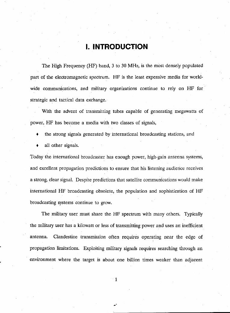
I. INTRODUCTION

The High Frequency (HF) band, 3 to 30 MHz, is the most densely populated

part of the electromagnetic spectrum. HF is the least expensive media for world

wide communications, and military organizations continue to rely on HF for·

strategic and tactical data exchange.

With the advent of transmitting tubes capable of generating megawatts of

power, HF has become a media with two classes of signals,

• the strong signals generated by international broadcasting stations, and

• all other signals.

Today the international broadcaster has enough power, high-gain antenna systems,

and excellent propagation predictions to ensure that his listening audience receives

a strong, clear signal. Despite predictions that satellite communications would make

international HF broadcasting obsolete, the population and sophistication of HF

broadcasting systems continue to grow.

The military user must share the HF spectrum with many others. Typically

the military user has a kilowatt or less of transmitting power and uses an· inefficient

antenna. Clandestine transmission often requires operating near the edge of

propagation limitations. Exploiting military signals requires searching through an

environment where the target is about one billion times weaker than adjacent

1

international broadcasting signals. Direct-sequence spread spectrum, frequency

hopping, and compressed-data burst modulations can complicate detection. The HF

listener will find every modulation type including voice, manual-morse, phase and

frequency-shift keying, facsimile, television, and pulse.

Today's best analog receivers can barely cope with the HF signal environment.

Trying to find new weak signals is hard enough, but the breadth of modulation

types requires large investments in analog detection hardware. Digital receiver

technology (i.e., receivers which change the analog radio-frequency (RF) voltage

into digital codewords prior to detection) promises to allow improvements in

detection.

The design of optimum, new-energy-detecting digital receivers requires an

understanding of the dynamics of the signal population. Until the 1980's there was

little, if any, data collection targeted on signal amplitude characteristics. Until

designers have data describing the signal environment, optimal receiver design is not

possible.

The first goal of this dissertation is to consolidate the separate HF spectrum

studies into a statistical description. The result proposes a probability distribution

function and places a range on values of the statistical moments.

The second goal is to develop a subset of the observations which describe

the military-type signal population. New observations verify the description of this

2

important signal subset. The data collection site is one of the Navy's Wullenweber

antenna facilities.

One can use the military-type signal descriptions to assess the performance

of HF receiver facilities. This dissertation proposes performance functions to

measure operational degradation. The resulting description projects the percentage

of signals-of-interest lost due to noise, interference, and signal-path attenuation.

The analog-to-digital converter is the key link in digital receiver performance.

This dissertation quantifies bounds on dynamic range resulting from the quantizer.

The results express the number-of-bits of dynamic range as a function of bandwidth

and other variables.

Other than the analog-to-digital converter itself, what other methods exist to

improve quantizing receiver performance? An overview shows which techniques

have potential for performance improvement.

Finally, this dissertation proposes a method of altering the voltage applied to

the quantizer. A way to accommodate the dynamic range required by the digital

receiver is by eliminating the signal or signals which are orders of magnitude

stronger than signals-of-interest.

This dissertation is organized in chapters concentrating on each of the topics

mentioned above. Within the chapters are original results of research including:

• Development of the first signal amplitude distribution function for the set of HF signals of military interest. Included are the first estimates for the mean and variance of this probability distribution.

3

• Verification of the signal amplitude distribution function by new observations of HF signals made at a European receiver site.

• Experimentation showing the effect on new signal detection caused by analog-to-digital converter saturation in a digital HF receiver.

• Development of the first HF receiver site performance criteria based on detailed HF signal observations.

• Development of the first HF receiver site performance criteria which details the differences between one and two ionospheric hop sites and between daytime and nighttime operation.

• First application of the new performance criteria to forms of man-made noise and signal path attenuation at a Navy CDAA receiver site. This allowed the best estimate to date of a receiver facility's performance in terms of percentage of signals lost.

• Derivation of the bounds on the dynamic range performance of a quantizer used in a wideband HF receiver system which shows that today's technology cannot meet the requirement.

• Description of a new technique to reduce the dynamic range requirement of the wideband HF receiver by eliminating the strongest signals.

Appendices provide an overview of collecting equipments, detail the newly collected

data, briefly describe the types of analog-to-digital converters, and show

MATHCAD computational work sheets.

4

II. HIGH FREQUENCY ENVIRONMENT

The High Frequency band is commonly known as shortwave (SW) radio. HF

is the frequency decade from 3 MHz to 30 MHz [Ref. 1]. Regardless of the

official designation, most spectrum users recognize HF as the span 1.7 MHz to 30

MHz. The lower-band limit is the edge of the medium wave AM broadcasting

band. Ionospheric propagation, which allows long-distance worldwide

communications, is the primary property which makes HF so important.

By international treaty, the International Telecommunications Union (ITU)

allocates the international aspects of spectrum usage. The intent is to provide

efficient allocation of limited spectrum and to minimize interference among

spectrum users. Within the HF band, the ITU allocates space to the following

services (with examples) [Ref. 2]:

• Fixed - radio communications between fixed land points (embassy to central government)

• Aeronautical Mobile - radio communications between an aircraft and a land station or between aircraft (air traffic control)

• Maritime Mobile - radio communications between a ship and a coastal station or between ships (public telegraph message service)

• Land Mobile - radio communications between a mobile land station and a stationary land station or between two mobile land stations (police dispatching)

5

• Aeronautical Radionavigation - determination of aircraft position for the purpose of navigation by means of the propagation properties of radio waves (Beacons)

• Maritime Radionavigation - determination of ship position for the purpose of navigation by means of the propagation properties of radio waves (LORAN)

• Radiolocation - determination of position for purposes other than those of navigation by means of the propagation properties of radio waves (Overthe-Horizon RADAR)

• Broadcasting - radio communications intended for direct reception by the general public (BBC World Service)

• Amateur - radio communications carried on by persons interested in radio technique solely with a personal aim without pecuniary interest (HAM radio)

• Earth-Space - radio communications between the earth and stations located beyond the earth's atmosphere (direct broadcast radio)

• Space - radio communications between stations beyond the earth's atmosphere (Tracking and Data Relay Satellite)

• Radio Astronomy - astronomy based on the reception of radio waves of cosmic origin

• Standard Frequency - radio transmissions on specified frequencies of stated high precision intended for general reception for scientific, technical, and other purposes (WWV, CHU, VNG, RWM, etc.).

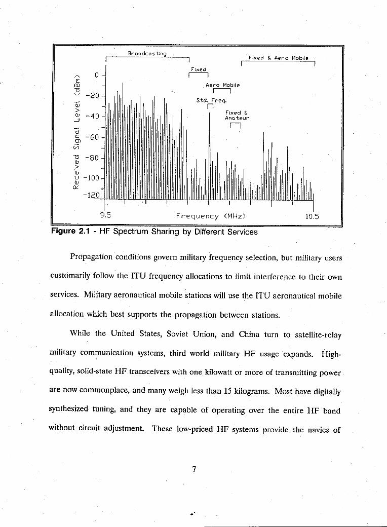
Figure 2.1 shows how services share HF frequency allocations. Usually one

service is considered primary; others are secondary on a not to interfere basis.

ITU regulations have over 1000 footnotes which allow treaty members to deviate

from strict spectrum allocation. In the footnotes most countries reserve the right

to use HF within their borders for governmental uses as needed.

6

Broo.dco.sting Fixed &. Aero Mobile

'" o -E

o:l <:5 '-/ -2 OJ > OJ -4

--1

o c -6 CJ)

V,)

<:5 -8 OJ > OJ u -10 OJ ~

-o -

-

o --

o --

0-

0-

--12 0

9.5

Fixed r-l

Aero Mobile r-l

Std. Freq. n

Fixed &. AMo.teur

n

II III II III lliili Frequency (MHz)

Figure 2.1 - HF Spectrum Sharing by Different Services

ul ~ I

10.5

Propagation conditions govern military frequency selection, but military users

customarily follow the lTU frequency allocations to limit interference to their own

services. Military aeronautical mobile stations will use the lTU aeronautical mobile

allocation which best supports the propagation between stations.

While the United States, Soviet Union, and China turn to satellite-relay

military communication systems, third world military HF usage expands. High-

quality, solid-state HF transceivers with one kilowatt or more of transmitting power

are now commonplace, and many weigh less than 15 kilograms. Most have digitally

synthesized tuning, and they are capable of operating over the entire HF band

without circuit adjustment. These low-priced HF systems provide the navies of

7

small nations with their only communications when out of line-of-sight of their

home base.

Within this crowded, growing signal environment, HF spectrum users must

deal with several important questions:

• What are the strongest signals?

• What is the minimum-detectable signal level or noise floor?

• What dynamic range must an HF receiver have?

A. STRONGEST SIGNALS

1. International Broadcasting

International broadcasting occupies the most crowded and rapidly

growing parts of the HF spectrum [Ref. 3]. Since the 1979 World Administrative

Radio Conference, HF broadcasting has expanded rapidly. HF remains a major

international broadcasting medium despite the enormous growth of satellite

communication systems.

Smaller countries can afford several 50 to 100 kilowatt HF transmitter

and simple antenna systems. A political leader can broadcast his message to the

world over HF. To large-land-area countries such as Brazil, Mexico, China;

Australia, and the Soviet Union, HF provides the least expensive way to broadcast

to their population. In the tropical areas, HF broadcasting often rivals medium

wave broadcasting because of lower atmospheric noise levels. In countries other

8

than the United States, most home and general-purpose radio receivers include a

few SW bands. [Ref. 3]

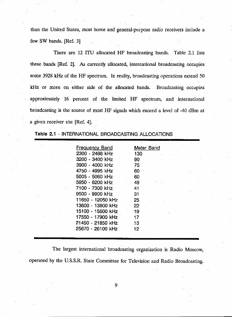
There are 12 ITU allocated HF broadcasting bands. Table 2.1 lists

these bands [Ref. 2]. As currently allocated, international broadcasting occupies

some 3928 kHz of the HF spectrum. In reality, broadcasting operations extend 50

kHz or more on either side of the allocated bands. Broadcasting occupies

approximately 16 percent of the limited HF spectrum, and international

broadcasting is the source of most HF signals which exceed a level of -40 dBm at

a given receiver site [Ref. 4].

Table 2.1 - INTERNATIONAL BROADCASTING ALLOCATIONS

Frequency Band 2300 - 2498 kHz 3200 - 3400 kHz 3900 - 4000 kHz 4750 - 4995 kHz 5005 - 5060 kHz 5950 - 6200 kHz 7100 - 7300 kHz 9500 - 9900 kHz 11650 - 12050 kHz 13600 - 13800 kHz 15100 - 15600 kHz 17550 - 17900 kHz 21450 - 21850 kHz 25670 - 26100 kHz

Meter Band 130 90 75 60 60 49 41 31 25 22 19 17 13 12

The largest international broadcasting organization is Radio Moscow,

operated by the U.S.S.R. State Committee for Television and Radio Broadcasting.

9

Radio Moscow publicly lists some 38 home or foreign service transmitter locations

within the U.S.S.R. with a published, combined transmitting power of 41.6 MW.

There are at least 95 more Soviet domestic HF broadcasting frequencies. Radio

Moscow has relay transmitters in Bulgaria, Cuba, and Mongolia. Adding to Radio

Moscow's coverage, the U.S.S.R. has 11 HF broadcasting stations operating in the

Soviet republics. [Ref. 3]

Most serious international broadcasters use multiple transmitters, power

levels of 250 to 1000 kilowatts, relay stations, and large curtain array antennas.

The British Broadcasting Corporation (BBC) World Service broadcasts 16 hours

daily to Australia, New Zealand, Papua New Guinea, and the Pacific Ocean area.

During certain hours, the BBC transmits on five frequencies to the Oceania target

area (15360, 11955, 9640, 7150, and 5975 kHz) from transmitter locations outside

the United Kingdom. The BBC uses HF relay stations in Singapore and Antigua,

with 250 kW transmitters at each site on each frequency. [Ref. 5]

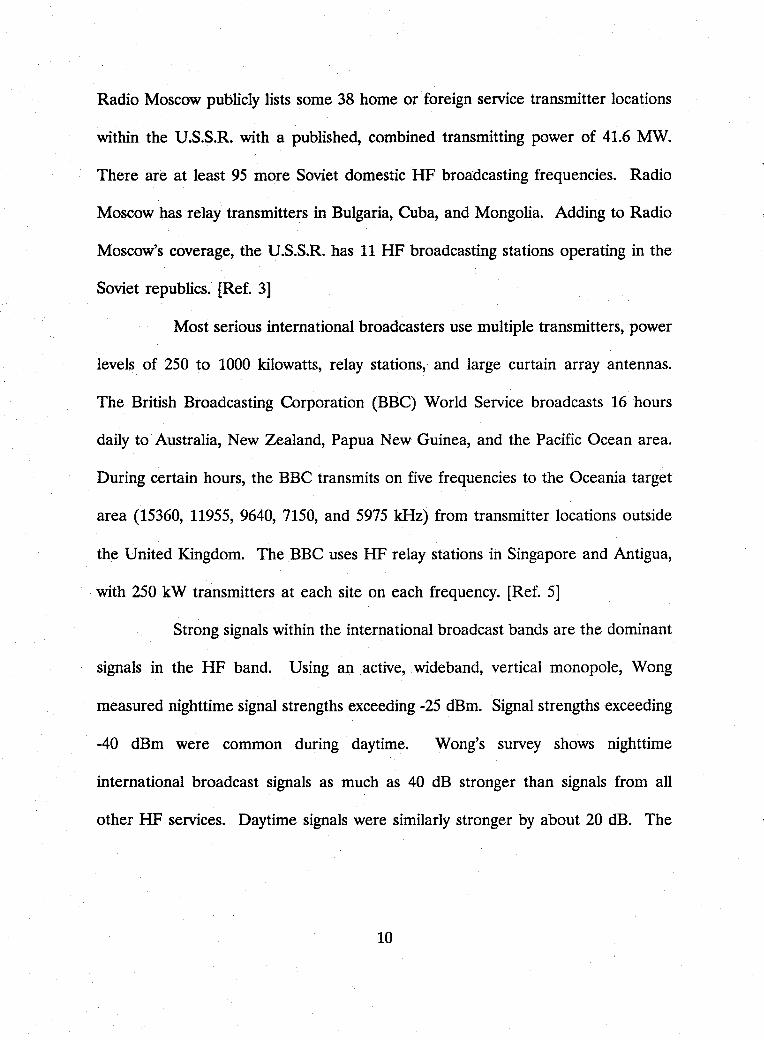
Strong signals within the international broadcast bands are the dominant

signals in the HF band. Using an active, wideband, vertical monopole, Wong

measured nighttime signal strengths exceeding -25 dBm. Signal strengths exceeding

-40 dBm were common during daytime. Wong's survey shows nighttime

international broadcast signals as much as 40 dB stronger than signals from all

other HF services. Daytime signals were similarly stronger by about 20 dB. The

10

absorption of ionospherically propagated signals by the ionospheric D layer accounts

for weaker daytime signals. [Ref. 4]

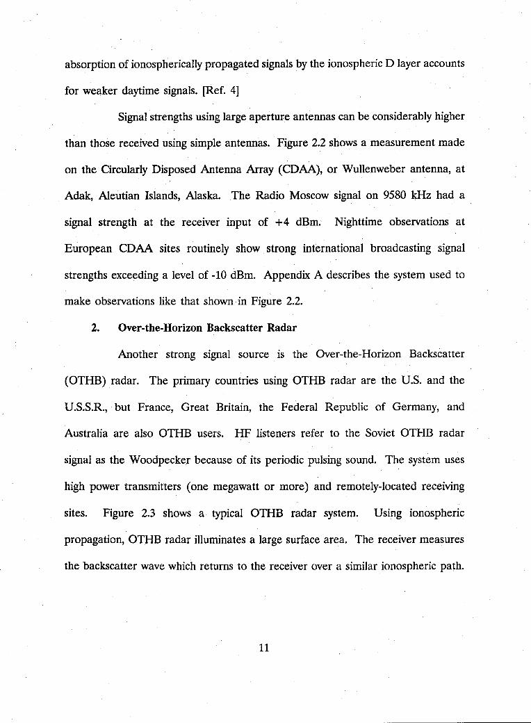
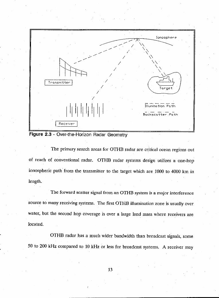
Signal strengths using large aperture antennas can be considerably higher

than those received using simple antennas. Figure 2.2 shows a measurement made

on the Circularly Disposed Antenna Array (CDAA), or Wullenweber antenna, at

Adak, Aleutian Islands, Alaska. The Radio Moscow signal on 9580 kHz had a

signal strength at the receiver input of +4 dBm. Nighttime observations at

European CDAA sites routinely show strong international broadcasting signal

strengths exceeding a level of -10 dBm. Appendix A describes the system used to

make observations like that shown in Figure 2.2.

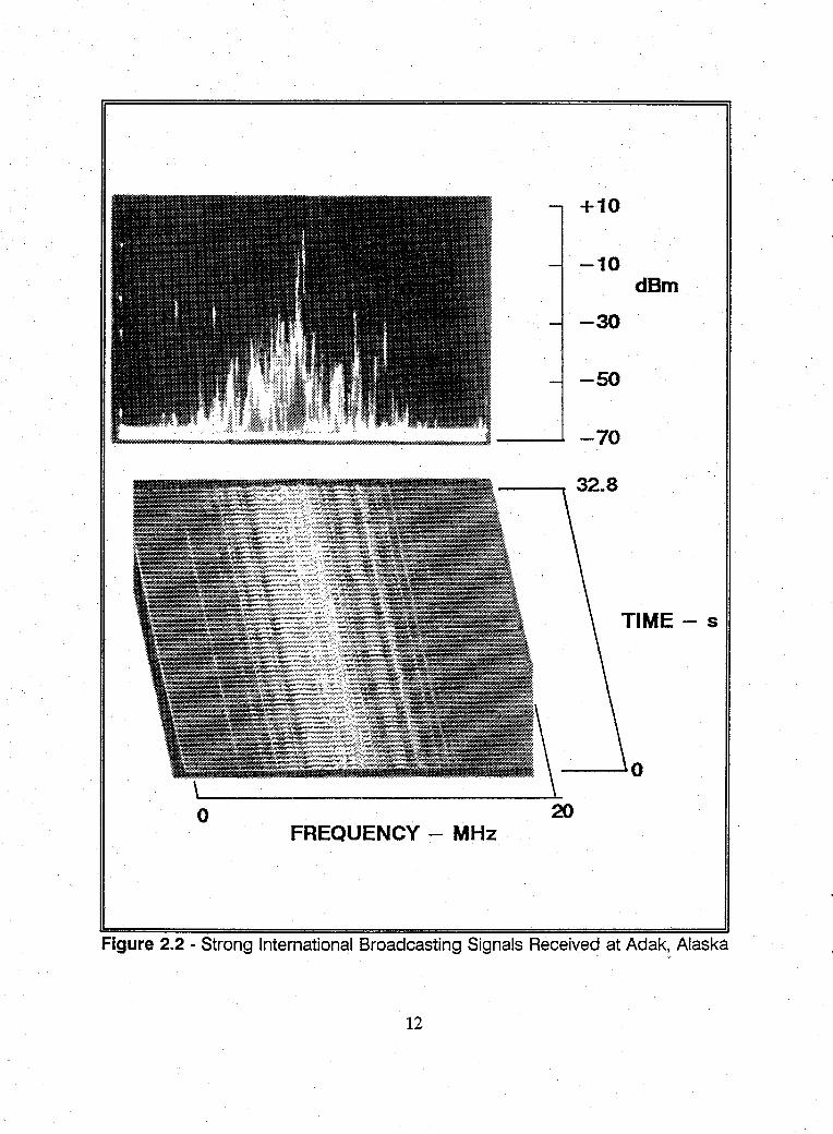
2. Over-the-Horizon Backscatter Radar

Another strong signal source· is the Over-the-Horizon Backscatter

(OTHB) radar. The primary countries using OTHB radar are the U.S. and the

U.S.S.R., but France, Great Britain, the Federal Republic of Germany, and

Australia are also OTHB users. HF listeners refer to the Soviet OTHB radar

signal as the Woodpecker because of its periodic pulsing sound. The system uses

high power transmitters (one megawatt or more) and remotely-located receiving

sites. Figure 2.3 shows a typical OTHB radar system. Using ionospheric

propagation, OTHB radar illuminates a large surface area. The receiver measures

the backscatter wave which returns to the receiver over a similar ionospheric path.

11

+10

-10 dBm

-30

-so

-70

TIME - s

--~o

o 20 FREQUENCY - MHz

Figure 2.2 - Strong International Broadcasting Signals Received at Adak~, Alaska

12

Ionosphere -- / -- " - I

;:--~

/

/

/

/

Tro.nSMitter I /

/ To.rget

/ /

1111111111111

llluMino. tion Po. th

Bo.cksc~tter Po.th

Receiver

Figure 2.3 - Over-the-Horizon Radar Geometry

The primary search areas for OTHB radar are critical ocean regions out

of reach of conventional radar. OTHB radar systems design utilizes a one-hop

ionospheric path from the transmitter to the target which are 1000 to 4000 km in

length.

The forward scatter signal from an OTHB system is a major interference

source to many receiving systems. The first OTHB illumination zone is usually over

water, but the second hop coverage is over a large land mass where receivers are

located.

OTHB radar has a much wider bandwidth than broadcast signals, some

50 to 200 kHz compared to 10 kHz or less for broadcast systems. A receiver may

13

have all of its passband filled with this pulsed OTHB energy. The residence time

for OTHB radars within a given allocation varies considerably. Observations show

that a typical OTHB radar signal resides on one frequency for durations lasting

from as short as two seconds to as long as two minutes.

Independent tests at numerous locations show that " ... the strength of

observed OTHB illumination did not appear to rival that of international broadcast

stations .... " [Ref. 6] This author's observations show otherwise. The OTHB radar

signal strength may reach the 0 dBm level on large aperture arrays. In particular,

the Soviet OTHB signal strength often exceeds the strongest international

broadcaster's signal strength.

3. Harmful Interference

Harmful interference, commonly called jamming, uses radio signals to

interfere deliberately with another radio transmission. Usually, the strongest HF

harmful-interference signals are those interfering with signals in the international

broadcasting bands.

Since World War II, most harmful interference to signals in the HF

broadcasting service originate within the U.S.S.R. Other countries jamming HF

broadcasting include Poland, Romania, Czechoslovakia, Bulgaria, China, Iraq, and

Iran. [Ref. 7]

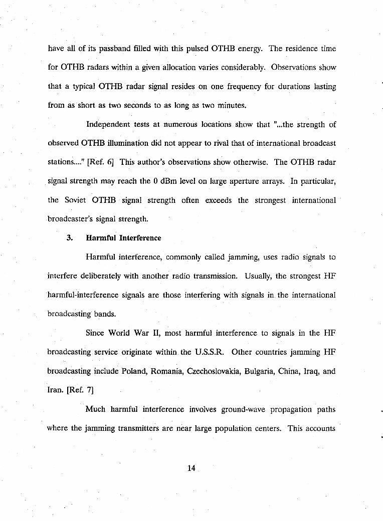
Much harmful interference involves ground-wave propagation paths

where the jamming transmitters are near large population centers. This accounts

14

for most of the identified jammers being in the western U.S.S.R. Figure 2.4 shows

the typical ground-wave interference geography.

DOD rD' :r~O~ DOD Local TransMitter

DOD

Dn D

o CJ 0 o CJ 0

-- --------

------

-----

DOD CJ CJ 0

Figure 2.4 - Local Harmful Interference Operations

-- DOD Cl 0 0

F.

ODD

.·

~ DOD

000 DB 0

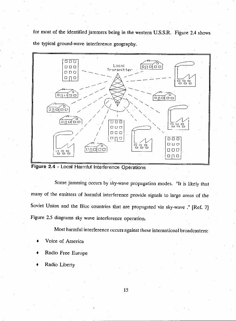
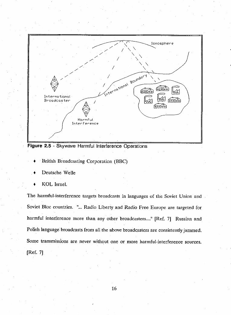
Some jamming occurs by sky-wave propagation modes. "It is likely that

many of the emitters of harmful interference provide signals to large areas of the

Soviet Union and the Bloc countries that are propagated via sky-wave ." [Ref. 7]

Figure 2.5 diagrams sky wave interference operation.

Most harmful interference occurs against these international broadcasters:

• Voice of America

• Radio Free Europe

• Radio Liberty

15

Interna tional Broadcaster

HarMful Interference

I

"-I '\ '\

'\. I '\\

'\ '\ '\

Figure 2.5 - Skywave Harmful Interference Operations

• British Broadcasting Corporation (BBC)

• Deutsche Welle

• KOL Israel.

Ionosphere

The harmful-interference targets broadcasts in languages of the Soviet Union and

Soviet Bloc countries. " ... Radio Liberty and Radio Free Europe are targeted for

harmful interference more than any other broadcasters ...... [Ref. 7] Russian and

Polish language broadcasts from all the above broadcasters are consistently jammed.

Some transmissions are never without one or more harmful-interference sources.

[Ref. 7]

16

With HF propagation, the harmful-interference signals also propagate

into non-target areas. Many harmful-interference stations simultaneously transmit

on the same frequency. The signal strengths are considerable, being greater than

many HF broadcasting signals. [Ref. 8]

Sky-wave jamming signal levels may exceed -29 dBm. Because of the

distribution of harmful-interference station location, most of the land mass of

Europe and Asia are within one ionospheric hop from the jamming transmitters.

Propagation conditions dictate that the broadcasters concentrate their transmissions

within three or four international broadcasting bands. Harmful-interference stations

usually concentrate on these same bands.

Since 1988, there has been a dramatic reduction in harmful-interference

signals, particularly from the U.S.S.R. However, the Soviet Union has not

dismantled the jamming facilities. The People's Republic of China began extensive

jamming of Voice of America signals during the Spring of 1989. China's jamming

coincided with the student demonstrations in Beijing. This demonstrates how

quickly a country can turn to harmful interference. During hostilities, harmful

interference will significantly contaminate HF spectrum, and receiver facilities

throughout the world will feel the impact of the jamming.

B. MINIMUM-DETECTABLE SIGNAL

The usual definition of minimum-detectable signal (MDS) is the presence of

a signal at least 3 dB above the received noise floor. The MDS will be different

17

for each receiver site and for each modulation system. In addition, the noise floor

will vary with sunspot cycle, season, time-of-day, and the activity of man-made noise

sources.

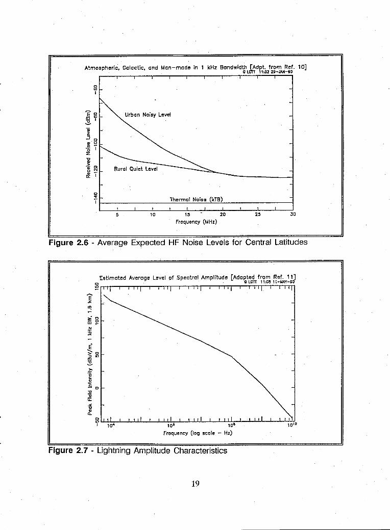
The ideal minimum noise floor is thermal noise, or the kTB noise level of

-144 dBm per kHz of bandwidth. HF energy-detection receivers using Fast Fourier

Transform spectral estimation techniques commonly use 1 kHz resolution

bandwidth. "Measurements have shown that spectral occupancy measurements are

approximately independent for frequency separations greater than 1 kHz." [Ref. 9]

A 1 kHz bandwidth is a common reference bandwidth.

At HF, the noise components which set a realistic noise baseline are:

• Atmospheric

• Galactic

• Man-made.

Figure 2.6, adapted from Sosin's review of CCIR Report 322, summarizes the

average effects of these noise sources. [Ref. 10]

1. Atmospheric Noise

Thunderstorm lightning discharges are the main source of HF

atmospheric noise. Figure 2.7 shows the spectral emission characteristics of

lightning noise. The line is the cubic-spline fit to data points from observations

made at many locations by many researchers. [Ref. 11]

18

Atmospheric, Galactic, and Man-made in 1 kHz Bandwidth rAdpt. from Ref. 10] o um \1:322g-.w/-90

o '" I

EO ID to "0 1 .......

~ 1r-----------------~~~~~~~----------------_4

30

Frequency (MHz)

Figure 2.6 - Average Expected HF Noise Levels for Central Latitudes

Estimated Average Level of Spectral Amplitude [Adopted from Ref. 111 o 0 LOTI 11;Cl\ II-l.IAY-.:S' ~nM~-r-r~~~-rrr~~~~--~~~~--rTTr~~-rrn

~~~~~~~~~~~~~~~~~~~--~~~~~~. 1 100 100

Frequency (log scole - Hz)

Figure 2.7 - Lightning Amplitude Characteristics

19

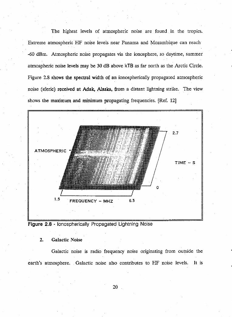
The highest levels of atmospheric noise are found. in the tropics.

Extreme atmospheric HF noise levels near Panama and Mozambique can reach

-60 dBm. Atmospheric noise propagates via the ionosphere, so daytime, summer

atmospheric noise levels lDay be 30 dB above kTB as far north as the Arctic Circle.

Figure 2.8 shows the spectral width of an ionospherically propagated atmospheric

noise (sferic) received at Adak, Alaska, from a distant lightning strike. The view

shows the maximum and minimum propagating frequencies. [Ref. 12]

2.7

ATMOSPHERIC

TIME - 5

o

1.5 FREQUENCY - MHZ 6.5

Figure 2.8 - lonospherically Propagated Lightning Noise

2. Galactic Noise

Galactic noise is radio frequency noise originating from outside the

earth's atmosphere. Galactic noise also contributes to HF noise levels. It is

20

strongest above 15 MHz, and it provides a background noise level about 20 dB

above kTB. [Ref. 1]

3. Man-made Noise

Man-made noise is potentially the strongest HF noise source. Itcomes

from many sources, including:

• Distribution Power Lines (Gap Noise)

.• Transmission Power Lines (Corona Noise and Gap Noise)

• Motor Vehicles (Ignition and Alternator Noise)

• Industrial Processes

• RF Stabilized Arc Welders

• Industrial, Scientific, and Medical (ISM) Signals (out-of-band)

• Digital System Noise (computers and digital communications)

• Nearby HF Transmitters.

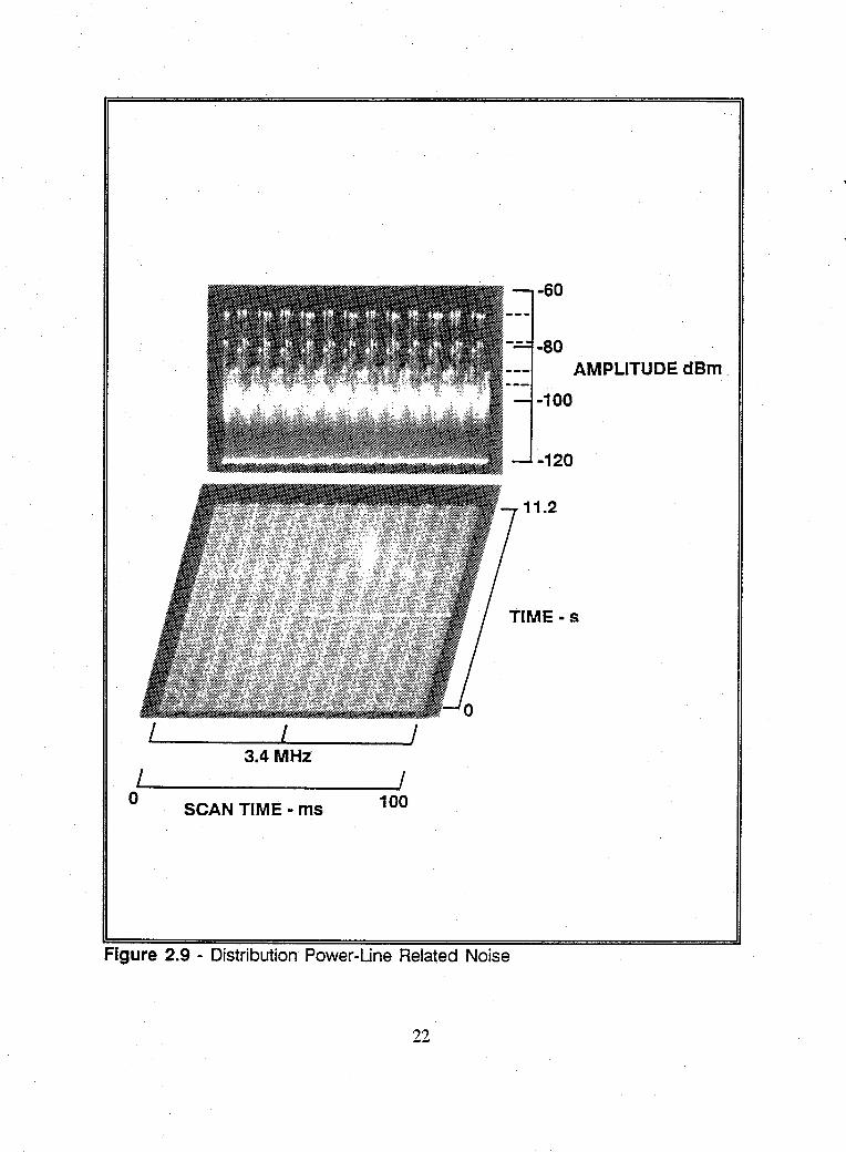
Many man-made noise sources are in line-of-site of the receiving

antenna. For example, Figure 2.9 shows noise from a nearby overhead distribution

power line. The peak noise level is -68 dBm in a 10 kHz bandwidth. "The most

bothersome type of noise found at most (HF) sites was that emanating from

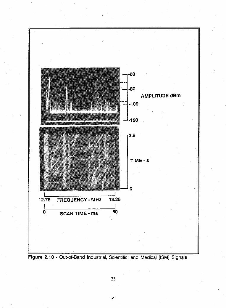
electric power lines." [Ref. 13] Other noise, such as ISM, can propagate into a

receiver site by ground-wave or by ionospheric modes of propagation. Figure 2.10

shows out-of-band ISM signals propagated by both means.

21

-60

AMPLITUDEdBm

-100

-120

TIME - s

~/ ________ I ______ ~1 3.4 MHZ

~/----------------~I o SCAN TIME _ ms 100

Figure 2.9 - Distribution Power -Une Related Noise

22

I I 12.75 FREQUENCY - MHz 13.25

1 I o SCAN TIME - ms 50

-60.

-80 AMPLITUDEdBm

-100

-120.

3.5

TIME - s

o

Figure 2.10 - Out-of-Band Industrial, Scientific, and Medical (ISM) Signals

23

Almost every HF receiver site will have some level and form of man-

made noise. Some types of man-made noise cover a bandwidth of 5 MHz or more,

while some have bandwidths of less than 10 kHz. Man-made noise also adds to

the overall power received, so it affects both the upper and lower dynamic range

limits of receiving systems.

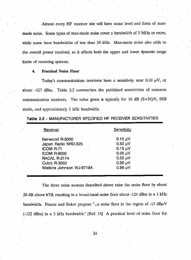
4. Practical Noise Floor

Today's communications receivers have a sensitivity near 0.10 Ii" V, or

about -127 dBm. Table 2.2 summarizes the published sensitivities of common

communication receivers. The value given is typically for 10 dB (S+ N)/N, SSB

mode, and approximately 3 kHz bandwidth.

Table 2.2 - MANUFACTURER SPECIFIED HF RECEIVER SENSITIVITIES

Receiver

Kenwood R-5000 Japan Radio NRD-525 ICOM R-71 ICOM R-9000 RACAL R-2174 Cubic R-3050 Watkins Johnson WJ-8718A

Sensitivity

0.15/lV 0.50/lV 0.15/lV 0.20/lV 0.25/lV 0.20/lV 0.56/lV

The three noise sources described above raise the noise floor by about

20 dB above kTB, resulting in a broad-band noise floor about -124 dBm in a 1 kHz

bandwidth. Pearce and Baker propose " ... a noise floor in the region of -15 dB~ V

(-122 dBm) in a 3 kHz bandwidth." [Ref. 14] A practical level of noise floor for

24

designing HF receiving systems, from antenna to receiver detector, should be at

least -125 dBm in a 3 kHz bandwidth.

C. OVERALL HF DYNAMIC RANGE REQUIREMENTS

HF receiving systems with large aperture antennas must be capable of

processing signal strengths as strong as -10 to 0 dBm without saturation. Signal

levels above 0 dBm will be infrequent, and such extreme signal levels will be highly

site dependent. The strongest signals will occur at night.

At Adak, Alaska, a receiver must be capable of processing a signal population

which spans 130 dB (strong signals as high as + 5 dBm to a noise floor of -125

dBm). Observations of signal population at CDAA receiver sites show that 120 dB

is the antenna-to-receiver dynamic range design goal.

Pierce and Baker reached a similar conclusion. "Reception of the weakest

signals, which may be as low as 0 dBp, V, requires a receiver with a signal handling

range of at least 120 dB (1 p, V to 1 V) .... " [Ref. 15]

Many of today's digitally operated HF receivers have front-end RF sections

which process the entire HF spectrum without pre-selection filtering. The RACAL

R-2174/U tri-service HF receiver covers 150 kHz to 30 MHz. The first stage RF

amplifier covers this entire span. Yet the R-2174/U does not have a front-end

amplifier with 120 dB dynamic range. The actual dynamic range is closer to 80 dB.

This means that signals received by the RACAL are subject to distortion from

25

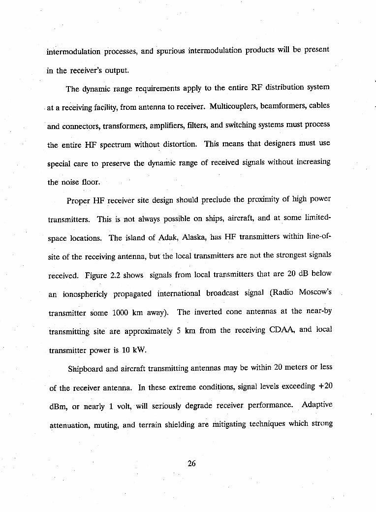
intermodulation processes, and spurious intermodulation products will be present

in the receiver's output.

The dynamic range requirements apply to the entire RF distribution system

at a receiving facility, from antenna to receiver. Multicouplers, beamformers, cables

and connectors, transformers, amplifiers, filters, and switching systems must process

the entire HF spectrum without distortion. This means that designers must use

special care to preserve the dynamic range of received signals without increasing

the noise floor.

Proper HF receiver site design should preclude the proximity of high power

transmitters. This is not always possible on ships, aircraft, and at some limited

space locations. The island of Adak, Alaska, has HF transmitters within line-of

site of the receiving antenna, but the local transmitters are not the strongest signals

received. Figure 2.2 shows signals from local transmitters that are 20 dB below

an ionosphericly propagated international broadcast signal (Radio Moscow's

transmitter some 1000 km away). The inverted cone antennas at the near-by

transmitting site are approximately 5 km from the receiving CDAA, and local

transmitter power is 10 kW.

Shipboard and aircraft transmitting antennas may be within 20 meters or less

of the receiver antenna. In these extreme conditions, Signal levels exceeding + 20

dBm, or nearly 1 volt, will seriously degrade receiver performance. Adaptive

attenuation, muting, and terrain shielding are mitigating techniques which strong

26

signal level environments require. This dissertation will not consider these special

install a tions.

27

III. HF SIGNAL AMPLITUDE STATISTICS

This dissertation will use the random variable vin as the root-mean

square (RMS) amplitude of the total, intercepted HF voltage applied to a receiver.

In a wideband receiver searching the HF spectrum for new signals, Vi n represents

a voltage comprised of all broadcast signals, non-broadcast signals, and noise.

Distortion in non-linear RF system components, losses in cables and connectors,

and induced noise add an undesired component to Vi n.

A wideband receiver and the first stages of many narrowband receivers must

be capable of processing the maximum peak value of vin• A narrowband receiver

with pre-selection will reject signals and noise outside the pre-selector bandwidth.

A much lower value of the input voltage will reach the front-end components of

a narrowband receiver with pre-selector filtering.

The RMS voltage produced only by signals of military interest is considerably

different than vin• It will have a smaller dynamic range than vin• Analog-to-digital

(AID) converters designed to optimally quantize signals of military interest should

not waste limited quantization dynamic range on the high amplitude broadcast band

signals. Instead, the AID design should optimize the ability to receive and process

the adversary's most clandestine transmitter.

28

A. HF SIGNAL STUDIES

As part of the Navy's Signal-to-Noise Enhancement Program, Prof. W. Ray

Vincent and LT John O'Dwyer estimated an initial distribution of HF signal

amplitudes. Using photographs taken of spectrum analyzer displays, they developed

an amplitude distribution function by counting the number of signals exceeding

threshold levels in 10 dB steps. This technique yielded a logarithmic distribution

with a slope of approximately 0.1 per 10 dB of signal amplitude change. [Ref. 16]

In 1980, Dutta and Gott studied HF spectrum occupancy to determine the

congestion levels. They compared the percentage of 1 kHz windows which had

signals with amplitude greater than threshold slicing levels. This data, when viewed

as an amplitude probability function, suggests a logarithmic distribution with a slope

of 0.15 per 5 dB change between -125 and -110 dBm. [Ref. 17]

In 1981, Wong and others conducted an HF spectral occupancy study which

provides spectrum occupancy information as a function of frequency. Their goal

was to predict the probability of finding a vacant frequency for military use. A

vacant frequency would have to have a signal level less than a specified amount.

Wong's data includes the percentage of time a 1 kHz bandwidth has a signal level

greater than specified thresholds. [Ref. 4]

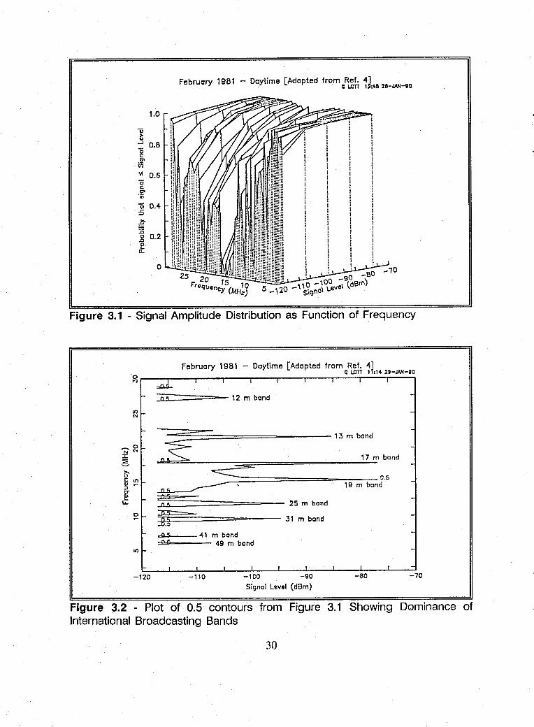
Figure 3.1 displays Wong's data differently from that used in Reference 4.

Figure 3.1 plots Wong's data as a two dimensional probability distribution of

frequency and the amplitude as a random variable. Figure 3.2 is a plot of the 0.5

29

February 1981 - Daytime [Adopted from Ref. 41 , C \.01T 12:45 26-JAN-DO

"ii ~

1.0

-J 0.8 ti c: 01 Vi '.I O.S o c: 01 'r;

-0 0.4-:5

~ :.0 ] 0.2

~ , :

o -SO O _iOO -~deff\)

5 \20 -i'. 01 \.e'Iel " -, SIgn

Figure 3.1 - Signal Amplitude Distribution as Function of Frequency

February 1981 - Daytime [Adopted from Ref. 41 c: \.01T 1 f:14 2g-JAN-DO

~~--~----~--~--~----~--~----~--~----.----,

-120

".Q.S...

:::loL:5s::::========- 12 m bond

--::::~~~~=====-------- 13 m bond

~~~ __ ~::::=s~=============-____ ~1~7~m bond

__ ===============~;::-:~:: O.S 19 m bond

~§§~========--- 25 m bond

~~~============~----:B.3 31 m band

dl 5 41 m band -!'5 49 m bond

-110 -100 -90

Signal level (d8m) -70

Figure 3.2 - Plot of 0.5 contours from Figure 3.1 Showing Dominance of International Broadcasting Bands

30

probability contours from the surface in Figure 3.1. It clearly shows the dominance

of signals in the international broadcasting bands. Nearly all signals exceeding the

0.5 contours are within ITU allocated broadcasting bands.

P.A. Bradley, analyzing Wong's data, concluded " ... that occupancy (or

congestion) varies with the threshold level (expressed in dBm) approximately in

accordance with a log-normal law." Of particular note is the limitation in Wong's

measurement system that allowed it to revisit each 1 kHz frequency window only

once every 3 to 5 days for one second duration. [Ref. 4]

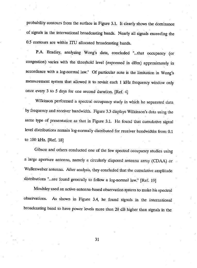
Wilkinson performed a spectral occupancy study in which he separated data

by frequency and receiver bandwidth. Figure 3.3 displays Wilkinson's data using the

same type of presentation as that in Figure 3.1. He found that cumulative signal

level distributions remain log-normally distributed for receiver bandwidths from 0.1

to 100 kHz. [Ref. 18]

Gibson and others conducted one of the few spectral occupancy studies using

a large aperture antenna, namely a circularly disposed antenna array (CDAA) or

Wullenweber antenna. After analysis, they concluded that the cumulative amplitude

distributions " ... are found generally to follow a log-normal law." [Ref. 19]

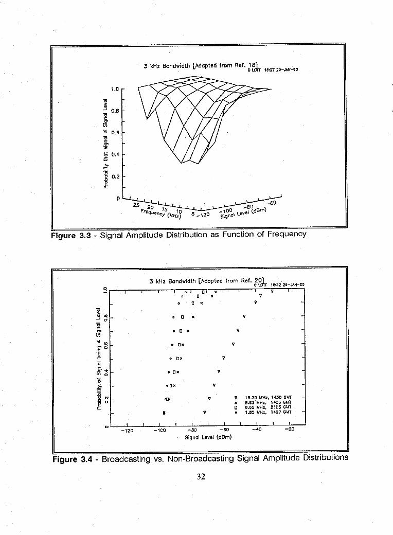
Moulsley used an active-antenna-based observation system to make his spectral

observations. As shown in Figure 3.4, he found signals in the international

broadcasting band to have power levels more than 20 dB higher than signals in the

31

a; >

1.0

~ O.B C c

~ \I O.S ""6 c C' ';;;

1] 0.4-:5

~ :c 1: 0.2 e 0..

o

:3 kHz Bandwidth [Adopted from Ref. 181 c Ul'rr 1:1:77 2g-JA)/-80


:3 kHz Bandwidth [Adopted from Ref. 201 G Ul'rr 1 e:J2 29-JA)/-90

~r---~--~---r--~--~D~~O~-~X-r--~--~r---~W--~I--~ D 0 X V •

o o )( V

0 0 x V

0 0 x V

0 Ox V

0 Ox V

o Ox V -

oOx V

«)( V V 15.25 MHz. 104.30 GMT )( 8.65 MHz. 1 «l5 GIlT 0 8.65 MHz. 2105 GIlT

I- • V 0 1.BS 101Hz. H27 CW -, I I i i i i i ...L ...L i

-120 -lOa -80 -60 -40 -20

Signal Level (dBm)

Figure 3.4 - Broadcasting vs. Non-Broadcasting Signal Amplitude Distributions

32

fixed, mobile, and maritime service bands. Moulsley's data shows an amplitude

cumulative probability distribution which follows a log-normal law. [Ref. 20]

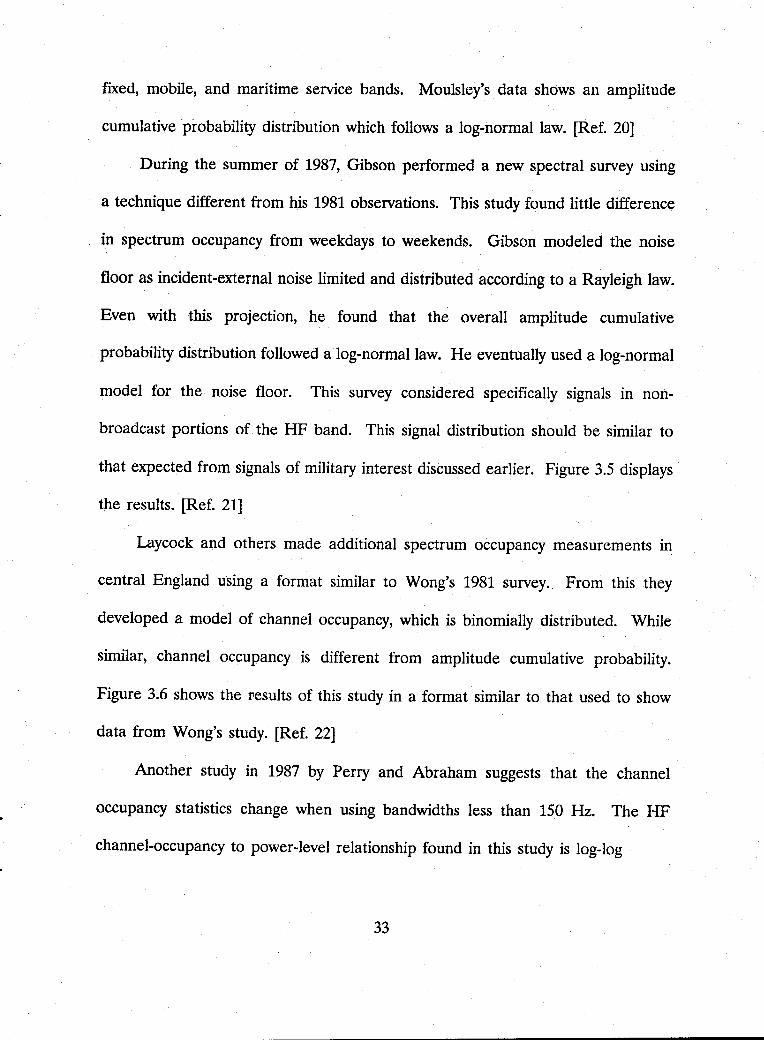
During the summer of 1987, Gibson performed a new spectral survey using

a technique different from his 1981 observations. This study found little difference

in spectrum occupancy from weekdays to weekends. Gibson modeled the noise

floor as incident-external noise limited and distributed according to a Rayleigh law.

Even with this projection, he found that the overall amplitude cumulative

probability distribution followed a log-normal law. He eventually used a log-normal

model for the noise floor. This survey considered specifically signals in non

broadcast portions of the HF band. This signal distribution should be similar to

that expected from signals of military interest discussed earlier. Figure 3.5 displays

the results. [Ref. 21]

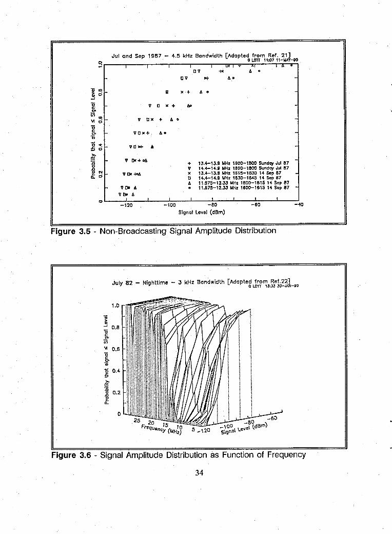
Laycock and others made additional spectrum occupancy measurements in

central England using a format similar to Wong's 1981 survey. From this they

developed a model of channel occupancy, which is binomially distributed. While

similar, channel occupancy is different from amplitude cumulative probability.

Figure 3.6 shows the results of this study in a format similar to that used to show

data from Wong's study. [Ref. 22]

Another study in 1987 by Perry and Abraham suggests that the channel

occupancy statistics change when using bandwidths less than 150 Hz. The HF

channel-occupancy to power-level relationship found in this study is log-log

33

q Jul and Sep 1987 - 4.5 kHz Bandwidth [Adapted from Ref. 21 ~

o LaTT 11:0711-11); -00 ,... .1 1 1 1 1 IJ<I "I I Il W

01 "'" to 0

01 Nt AD -"ii III a x + to 0 -~ 0 -I

"0 1 0 x + lP -c .!<' VI II>

V Ox + 6 0 -\1 0 "0 c

VDx+ 11.0 -0> '0;

cot-:50 VO WI- • -~ v [)(+06 -:c + 13.4-13.9 104Hz 1600-1800 Sunday Jul 87 0 .c V 14.4-1 .... 8 101Hz lS00-18OO Sunday Jul 87 e N V [)( -lOA x 13.4-13.8 101Hz 1615-1SJO 14 Sep 87 -D.. 0 0 14.4-14.9 101Hz 1530-1&45 ,... Sep 87

to 11.975-12.33 101Hz 1800-1815 ,... Sep 87 V [)II A 0 11.975-12.33 101Hz 1600-1615 ,... Ssp 87 -

V 91 A 0 1 1 1 I I I , ,

-120 -100 -80 -60 --«)

Signal Level (dSm)

Figure 3.5 -Non-Broadcasting Signal Amplitude Distribution

July 82 - Nighttime - :3 kHz Bandwidth [Adopted from Ref.221 C LCTT 13;3;) 30-J.':h-;o

1.0

a; > ~ O.B "0 c ~ \4 O.S '6 c 0>

'0;

'0 0.4-£i

~ :0 .8 0.2 I: a..

o F. 20 15 . reqollncy (I.tH~~ 5 ... ,20


34

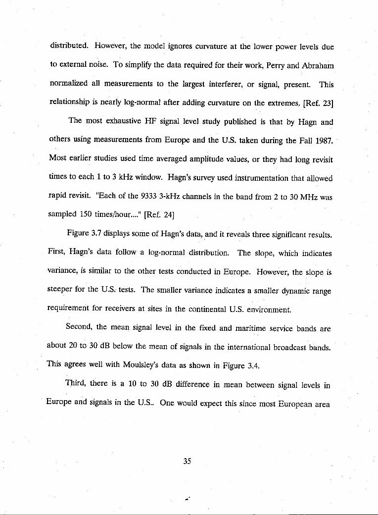
distributed. However, the model ignores curvature at the lower power levels due

to external noise. To simplify the data required for their work, Perry and Abraham

normalized all measurements to the largest interferer, or signal, present. This

relationship is nearly log-normal after adding curvature on the extremes. [Ref. 23]

The most exhaustive HF signal level study published is that by Hagn and

others using measurements from Europe and the U.S. taken during the Fall 1987 ..

Most earlier studies used time averaged amplitude values, or they had long revisit

times to each 1 to 3 kHz window. Hagn's survey used instrumentation that allowed

rapid revisit. "Each of the 9333 3-kHz channels in the band from 2 to 30 MHz was

sampled 150 timeslhour .... " [Ref. 24]

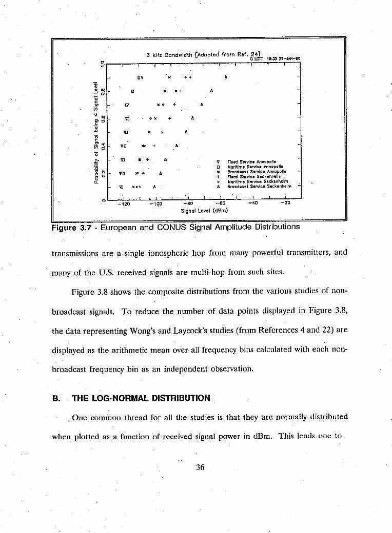
Figure 3.7 displays some of Hagn's data, and it reveals three significant results.

First, Hagn's data follow a log-normal distribution. The slope, which indicates

variance, is similar to the other tests conducted in Europe. However, the slope is

steeper for the U.S. tests. The smaller variance indicates a smaller dynamic range

requirement for receivers at sites in the continental U.S. environment.

Second, the mean signal level in the fixed and maritime service bands are

about 20 to 30 dB below the mean of signals in the international broadcast bands.

This agrees well with Moulsley's data as shown in Figure 3.4.

Third, there is a 10 to 30 dB difference in mean between signal levels in

Europe and signals in the U.S.. One would expect this since most European area

35

:3 kHz 8andwidth [Adapted from Ref'l~ le:~ 2;-'IAN-&O

~~--~~r-~~~---'I---'I--~---'t---'I--~---'---'

0 .. " 0+ A -

II )( 0+ A -

I:V )( 0 + A

';[] 0)( + A

';[] • + A

VO )0 + A

';[] • + A V Flxed Service Annapone 0 Maritim. Service Annapolis

VO )0+ A )( Broadcc~t Service Annapolis -+ Flxed Service Seckenhelm 0 lAaritime Service Seckenhelm

';[] ,,0+ A A Broadcoel Service Seckenn.lm -, I I I i l

-120 -100 -80 -SO -40 -20

Signcl Level (dBm)

Figure 3.7 - European and CONUS Signal Amplitude Distributions

transmissions are a single ionospheric hop from many powerful transmitters, and

many of the U.S. received signals are multi-hop from such sites.

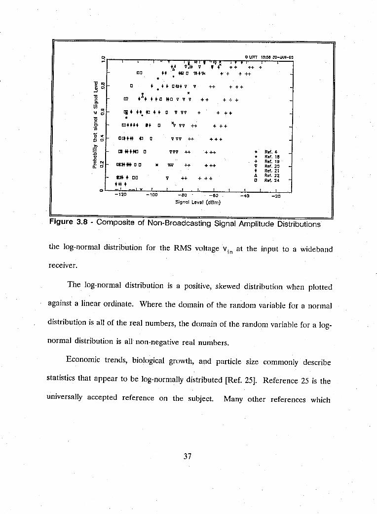
Figure 3.8 shows the composite distributions from the various studies of non-

broadcast signals. To reduce the number of data points displayed in Figure 3.8,

the data representing Wong's and Laycock's studies (from References 4 and 22) are

displayed as the arithmetic mean over all frequency bins calculated with each non-

broadcast frequency bin as an independent observation.

B. THE LOG-NORMAL DISTRIBUTION

One common thread for all the studies is that they are normally distributed

when plotted as a function of received signal power in dBm. This leads one to

36

o

c++ + c~+ v v ++ + ++

++ + '" +

Ii + + +. (l • + c v vv + + + + o

m++++ U c ~ vv ++ + ++

v vv ++ +++

vvv ++ + ++

tnt ... CD

f- Q + 00

++t +

Wi ++ +++

V ++ -I- + +

--

--

o R.t.4 • Ref. IS + Ref. 19 V Ref. 20 • Ref. 21 I!. Rat. 22 C 1W.24

o~~~~~Y~~ __ ~ __ ~~~~I ___ ~i __ ~I __ ~I~~~ -120 -100 -BO -60 -40 -20

Signal Level (dBm)

Figure 3.8 - Composite of Non-Broadcasting Signal Amplitude Distributions

the log-normal distribution for the RMS voltage Yin at the input to a wideband

receIver.

The log-normal distribution is a positive, skewed distribution when plotted

against a linear ordinate. Where the domain of the random variable for a normal

distribution is all of the real numbers, the domain of the random variable for a log-

normal distribution is all non-negative real numbers.

Economic trends, biological growth, and particle size commonly describe

statistics that appear to be log-norma]]y distributed [Ref. 25]. Reference 25 is the

universally accepted reference on the subject. Many other references which

37

mention the log-normal distribution simply summarize the Aitchison and Brown

[Ref. 25] work.

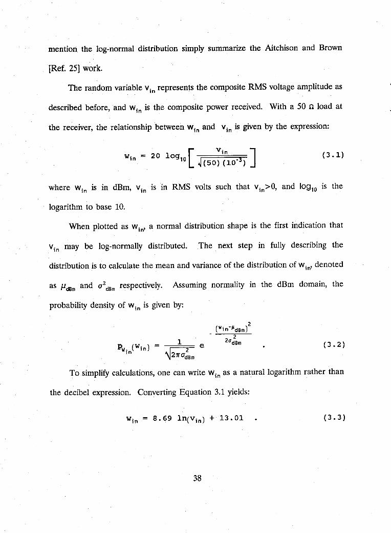
The random variable vin represents the composite RMS voltage amplitude as

described before, and Win is the composite power received. With a 50 n load at

the receiver, the relationship between Win and v in is given by the expression:

= 20 log [ Vi n ] 10 ~(50)(10-3)

(3.1)

where Win is in dBm, Vin IS In RMS volts such that vin>O, and 10910 is the

logarithm to base 10.

When plotted as Win' a normal distribution shape is the first indication that

Vin may be log-normally distributed. The next step in fully describing the

distribution is to calculate the mean and variance of the distribution of Win' denoted

as f..ldBm and (]2 dBm respectively. Assuming normality in the dBm domain, the

probability density of Win is given by:

(3.2)

To simplify calculations, one can write Win as a natural logarithm rather than

the decibel expression. Converting Equation 3.1 yields:

(3.3)

38

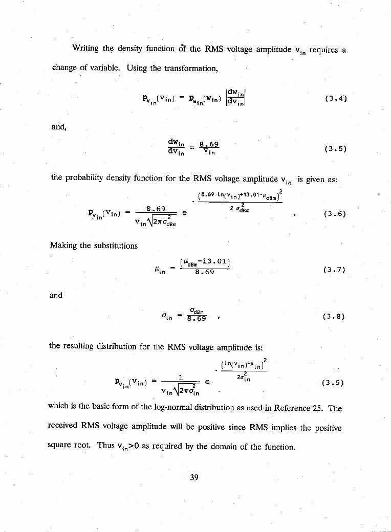
Writing the density function of the RMS voltage amplitude vin requires a

change of variable. Using the transformation,

and,

dWin = 8.69 dvo -V-,on ,n

(3.4)

(3.5)

the probability density function for the RMS voltage amplitude vin is given as:

(8.69 In(Vin)+13.01-#dBm)2

Making the substitutions

ILln =

and

(J..£dBm-13 • 01 ) 8.69

,

2 2 O'dBm

the resulting distribution for the RMS voltage amplitude is:

(3.6)

(3.7)

(3.8)

(3.9)

which is the basic form of the log-normal distribution as used in Reference 25. The

received RMS voltage amplitude will be positive since RMS implies the positive

square root. Thus vin>O as required by the domain of the function.

39

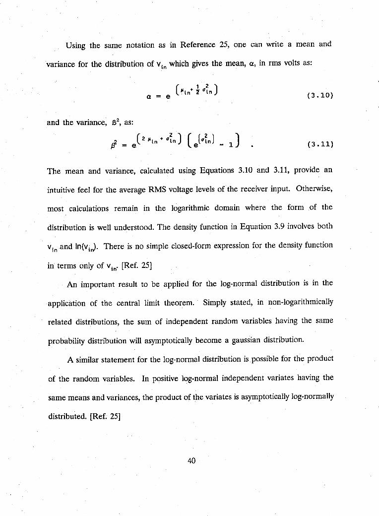
Using the same notation as in Reference 25, one can write a mean and

variance for the distribution of Vi n which gives the mean, a, in rms volts as:

(3.10)

and the variance, S2, as:

If = e ( 2 IL ln + q~n) (e( q~n) - 1) (3.11)

The mean and variance, calculated using Equations 3.10 and 3.11, provide an

intuitive feel for the average RMS voltage levels of the receiver input. Otherwise,

most calculations remain in the logarithmic domain where the form of the

distribution is well understood. The density function in Equation 3.9 involves both

vin and In(vin). There is no simple closed-form expression for the density function

in terms only of Vi n' [Ref. 25]

An important result to be applied for the log-normal distribution is in the

application of the central limit theorem. Simply stated, in non-logarithmically

related distributions, the sum of independent random variables having the same

probability distribution will asymptotically become a gaussian distribution.

A similar statement for the log-normal distribution is possible for the product

of the random variables. In positive log-normal independent variates having the

same means and variances, the product of the variates is asymptotically log-normally

distributed. [Ref. 25]

40

This can be an important tool in estimating the products of the random

variable vin caused by non-Iinearities in the RF system. These products are the

resulting intermodulation products which add as noise to the desired signal.

C. ESTIMATING MEAN AND VARIANCE

The problem here is to match an experimentally determined cumulative

probability distribution function or probability density function to a theoretical

function. The two dependent variables to be applied in the match are the mean

and variance. To simplify calculations, the matching for HF signal studies is done

in dBm. The goal is to match a normal distribution to the experimental

observations. The following summarizes the mean and variance estimation methods.

1. Quartile Estimation

A simple method exists to fit a normal probability density function to

an experimentally derived histogram based on quartiles. Let N be the total number

of observations. The observations are ordered in histogram form. Starting with the

ordinate having the smallest value, the first quartile is the ordinate value

corresponding to N/4 observations, etc. Stated differently, the first quartile is the

ordinate value for which one-fourth of the observations have a value less than or

equal that ordinate. The second, third, and fourth quartiles have similar definitions.

The second quartile is the observational median.

Croxton used a quartile rule to provide an estimate of the mean and

standard deviation of fitting a normal density based on these quartiles. [Ref. 26]

41

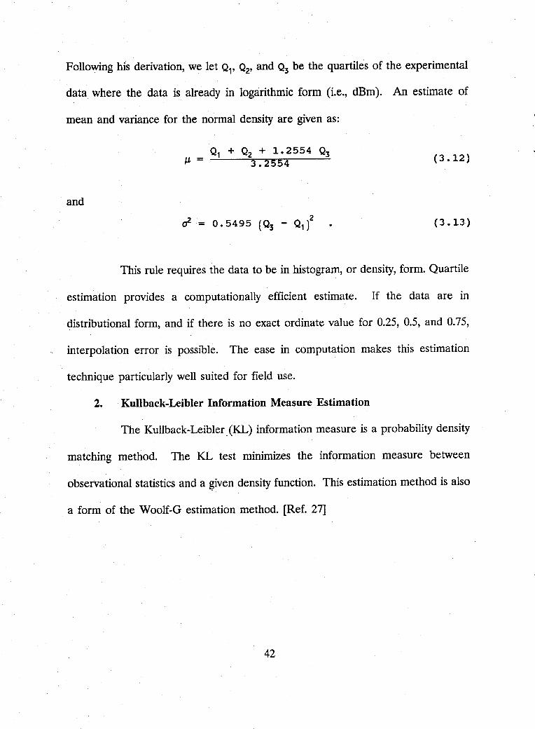
Following his derivation, we let Q" Qz' and Q3 be the quartiles of the experimental

data where the data is already in logarithmic form (i.e., dBm). An estimate of

mean and variance for the normal density are given as:

Q, + Qz + 1. 2554 Q3 J.L = 3.2554 (3.12)

and

(3.13 )

This rule requires the data to be in histogram, or density, form. Quartile

estimation provides a computationally efficient estimate. If the data are in

distributional form, and if there is no exact ordinate value for 0.25, 0.5, and 0.75,

interpolation error is possible. The ease in computation makes this estimation

technique particularly well suited for field use.

2. Kullback-Leibler Information Measure Estimation

The Kullback-Leibler(KL) information measure is a probability density

matching method. The KL test minimizes the information measure between

observational statistics and a given density function. This estimation method is also

a form of the Woolf-G estimation method. [Ref. 27]

42

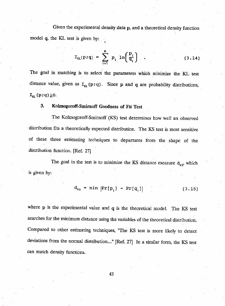
Given the experimental density data p, and a theoretical density function

model q, the KL test is given by:

m

IKL(p;q) = L Pi In( ~: ) i=1

(3.14)

The goal in matching is to select the parameters which minimize the KL test

distance value, given as IKL (p; q). Since p and q are probability distributions,

IKL (p; q) ~o.

3. KolmogorofT-SmirnofT Goodness of Fit Test

The Kolmogoroff-Smirnoff (KS) test determines how well an observed

distribution fits a theoretically expected distribution. The KS test is most sensitive

of these three estimating techniques to departures from the shape of the

distribution function. [Ref. 27]

The goal in the test is to minimize the KS distance measure d KS' which

is given by:

(3 • 15)

where p is the experimental value and q is the theoretical model. The KS test

searches for the minimum distance using the variables of the theoretical distribution.

Compared to other estimating techniques, "The KS test is more likely to detect

deviations from the normal distribution .... " [Ref. 27] In a similar form, the KS test

can match density functions.

43

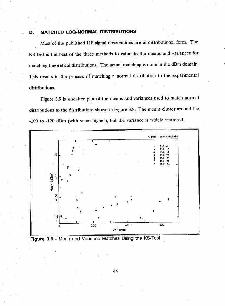
D. MATCHED LOG-NORMAL DISTRIBUTIONS

Most of the published HF signal observations are in distributional form. The

KS test is the best of the three methods to estimate the means and variances for

matching theoretical distributions. The actual matching is done in the dBm domain.

This results in the process of matching a normal distribution to the experimental

distributions.

Figure 3.9 is a scatter plot of the means and variances used to match normal

distributions to the distributions shown in Figure 3.8. The means cluster around the

-100 to -120 dBm (with some higher), but the variance is widely scattered.

GLOlT 13:35 8-Ft:B-90

I I I I I I

V + " nor. 4

+ • Rof. Ie 0 + + R"r. 19 'fr- V Ref. 20 -

+ Ror. 21 lJ. Rof.22

I- :t 0 Rof.24 -v

E'g r- v -~I V V ....., c 0 I- -III

::!:

0 0

~I- • • -I 0 • • + • •

l- • • -• • •

~ ~ • • i .. -I

I I 1 I I I

0 200 -100 GOO Variance

Figure 3.9 - Mean and Variance Matches Using the KS-Test

44

Most of the observations include day and night measurements. One should

expect a smaller daytime mean ancl a larger nighttime mean and variance.

One can define a dynamic range requirement as the one percent to the 99

percent points on the distribution. Figure 3.10 is an example distribution using a

-110 dBm mean and a variance of 100. This distribution leads to a design dynamic

range of about 55 dB, and it shows the relatively small dynamic range of the

received signals when one considers only signals of military interest.

C LOTI 13:54 e-fEB-90 ~~--~---.----r---~---.~--.----.---.----.---~

o~~~ __ ~ _____ ~ __ ~ __ ~ _____ ~ __ -L ___ ~ _____ ~ __ ~

-140 -120 -100 -80 -00 -40

Signol Level (dBm)

Figure 3.10 - Example Signal-ot-Interest Distribution

45

IV. HF NEW-ENERGY OBSERVATIONS

The generalized, search receiver observes the entire HF spectrum and detects

the presence of new energy. This new energy may be noise, a signal of interest,

or another signal. The search receiver screens new energies using generalized

parameters to create a set of new energies. These may include a subset consisting

of signals of interest.

The search receiver decides if new energy is present based on certain

measurements. Once screened, the search system assigns an analysis receiver to

identify the new energy as a possible signal of interest. There are so many rapidly

changing events in the HF spectrum that new-energy detection can, at times, be

unmanageable.

When viewed as a composite voltage seen by the receiver, a voltage change

alone is not an adequate indicator of a possible signal. The new-energy decision

requires changes in measurable parameters including:

• Amplitude change exceeding a programmed threshold

• Duration

• Center frequency

• Bandwidth

46

• Identifiable frequency components (i.e., two specific frequencies used in frequency-shift keying)

• Identifiable temporal variations (i.e., spacing of amplitude-shift keying).

A new-energy system observes the entire HF spectrum before making new-energy

decisions. The system usually uses an omnidirectional antenna system to allow

reception from all directions.

A wideband receiving system rapidly samples the entire 2 to 30 MHz band,

transforms the voltage into the frequency domain, and checks each frequency bin

against programmed parameters. If the latest observation meets certain criteria,

new energy is assumed to be present. There are usually many new energies present

in each observation. The wideband system then assigns an analysis receiver to each

new energy.

A narrowband new-energy system incorporates a different search approach.

The system tunes a narrow-bandwidth receiver to a specific frequency, determines

if a signal is present, and compares the frequency to a previously monitored

frequency list. The frequency of the narrowband receiver may come from an

established search list, or the frequency selection may be by a random process. If

new energy is present, the same receiver used for new-energy detection becomes

the analysis receiver by adding parameter recognizers as mentioned earlier.

The narrowband system can use either an omnidirectional or beam antenna

depending on how well one can a priori define the geographic search area. The

receiver component of the narrowband system is a typical HF communications

47

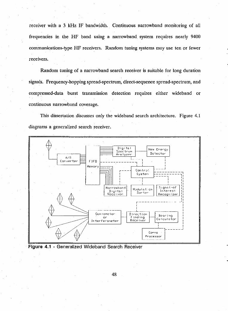
receiver with a 3 kHz IF bandwidth. Continuous narrowband monitoring of all

frequencies in the HF band using a narrowband system requires nearly 9400

communications-type HF receivers. Random tuning systems may use ten or fewer

receivers.

Random tuning of a narrowband search receiver is suitable for long duration

signals. Frequency-hopping spread-spectrum, direct-sequence spread-spectrum, and

compressed-data burst transmission detection requires either wideband or

continuous narrowband coverage.

This dissertation discusses only the wideband search architecture. Figure 4.1

diagrams a generalized search receiver.

AID Converter

Dig I to. I SpectruP'l Ano.lYZE'r

'----l FIFO ------------, I

I I I

GonloP'leter Or

Interf'E'rOP'letE'r

___ J

---------, ====::;-----'1 '----..----' I : I

I II ,------'-----, I I

Slgnol-of'11 Interest II

II Recogn I zer I I

II I

I---------------~I I I I I

I I

Beo.rlng I

Colculo.tor :

COP'lP'lS Processor

I I _____ ...1

Figure 4.1 - Generalized Wide band Search Receiver

48

A. EXAMPLES OF NEW ENERGIES REQUIRING SEARCH SCREENING

There are thousands of potential HF new energies per second. The following

are examples of potential new-energy events which require search screening. This

list represents the large class of new energies, and it includes many noise sources

discussed in Chapter II.

1. Sferics

Sferic is a term used to describe short burst of atmospheric

electromagnetic energy. Convective, cumulonimbus cloud thunderstorm discharges

account for nearly all sferics. Lightning associated with volcanic eruptions is the

other source of sferics.

The average duration of a lightning stroke is approximately 30 J,LS, and

each lightning flash averages four strokes. In a hemispheric satellite view, there is '

an average of 1000 thunderstorms visible, centered primarily in the tropics.

Worldwide, an estimated 400 lightning strokes occur each second. With an average

power per stroke of 1013 watts, each stroke can generate significant energy in the

HF spectrum. [Ref. 28]

Since more storms containing lightning occur in the tropics, sferic energy

is maximum in these regions. Sferic energy also propagates over ionospheric paths

to far distant receivers.

49

Sferics are broadband, and each event lasts about 100 to 200 ms. These

two characteristics, bandwidth and duration, can form a screening criteria in the

search receiver to minimize new-energy decisions from sferics.

2. Broadband Man-Made Noise

Chapter II discusses numerous types of broadband man-made noise.

The key to search screening is the broadband character. Broadband noise, from

any source, will increase the noise floor and prevent weak signal reception.

Of particular concern is switching noise generated by RF switching

systems employing digitally-controlled diode switches in matrix regimes. Switching

transients caused by turning on and off the diodes in the switching matrix appear

as new energy. For optimum performance, there should be no switching or other

transient generating devices between the antenna and the search receiver.

Switching noise is not necessarily broadband, so new-energy screening may be

difficult.

3. Industrial, Scientific, and Medical (ISM) Noise

International agreements permit the operation of ISM devices in certain

frequency bands. Yet, evidence shows that out-of-band ISM interference is

increasing at receiver sites throughout the world. Many ISM signals are propagated

by ionospheric modes to distant receiver sites.

A typical ISM signal appears as a repetitive signal which may sweep over

a frequency band. ISM signal bandwidths range from a few kHz to hundreds of

50

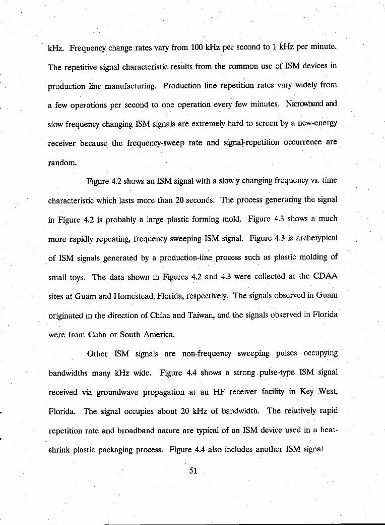
kHz. Frequency change rates vary from 100 kHz per second to 1 kHz per minute.

The repetitive signal characteristic results from the common use of ISM devices in

production line manufacturing. Production line repetition rates vary widely from

a few operations per second to one operation every few minutes. Narrowband and

slow frequency changing ISM signals are extremely hard to screen by a new-energy

receiver because the frequency-sweep rate and signal-repetition occurrence are

random.

Figure 4.2 shows an ISM signal with a slowly changing frequency vs. time

characteristic which lasts more than 20 seconds. The process generating the signal

in Figure 4.2 is probably a large plastic forming mold. Figure 4.3 shows a much

more rapidly repeating, frequency sweeping ISM signal. Figure 4.3 is archetypical

of ISM signals generated by a production-line process such as plastic molding of

small toys. The data shown in Figures ~.2 and 4.3 were collected at the CDAA

sites at Guam and Homestead, Florida, respectively. The signals observed in Guam

originated in the direction of China and Taiwan, and the signals observed in Florida

were from Cuba or South America.

Other ISM signals are non-frequency sweeping pulses occupying

bandwidths many kHz wide; Figure 4.4 shows a strong pulse-type ISM signal

received via groundwave propagation at an HF receiver facility in Key West,

Florida. The signal occupies about 20 kHz of bandwidth. The relatively rapid

repetition rate and broadband nature are typical of an ISM device used in a heat

shrink plastic packaging process. Figure 4.4 also includes another ISM signal

51

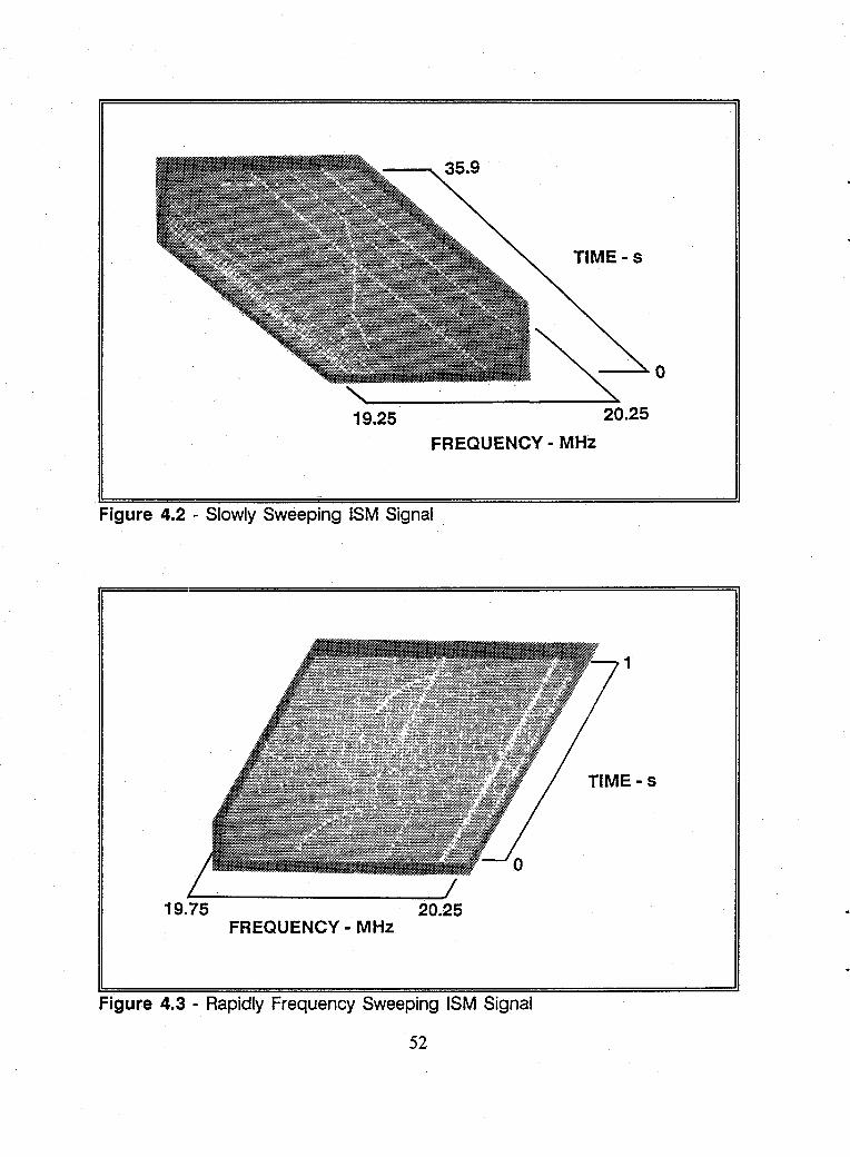
TIME - s

o

19.25 20.25

FREQUENCY - MHz

Figure 4.2 - Slowly Sweeping ISM Signal

1

TIME - s

19.75 20.25 FREQUENCY - MHz

Figure 4.3 - Rapidly Frequency Sweeping ISM Signal

52

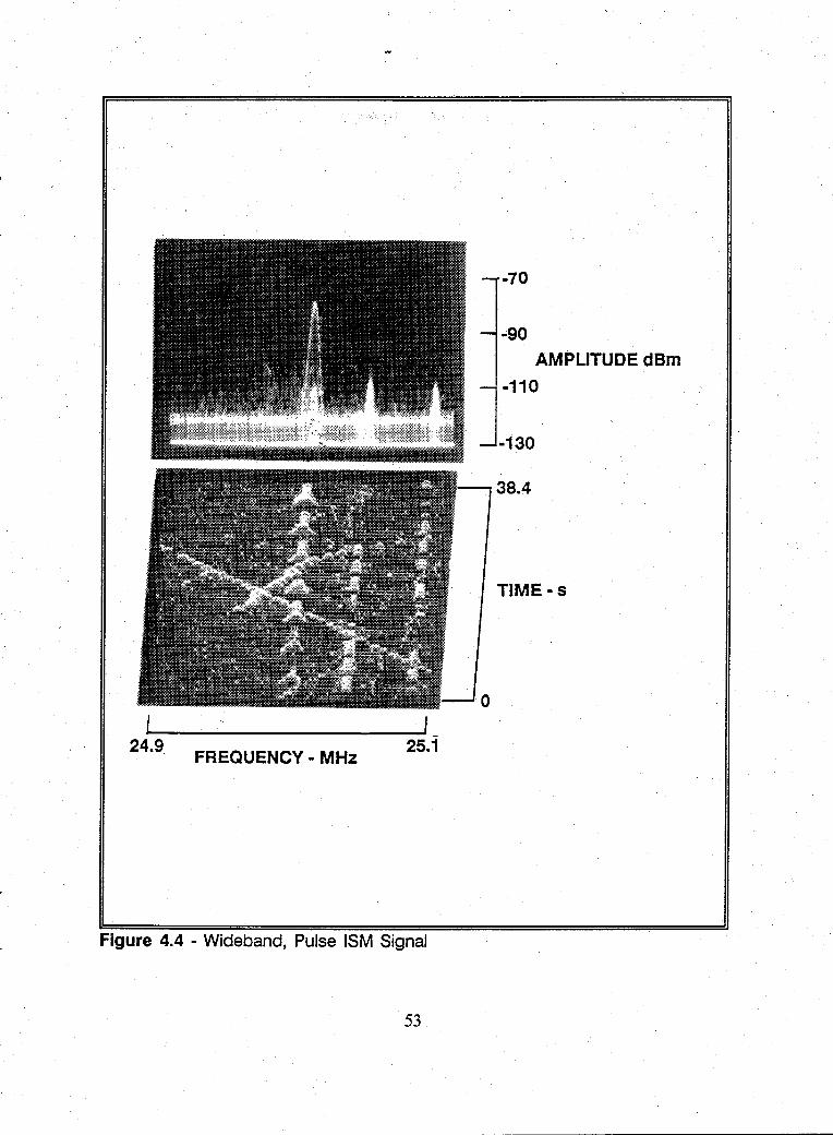
~------------------~'-24.9 FREQUENCY· MHz

25.1

Figure 4.4 - Wideband, Pulse ISM Signal

53

·70

·90 AMPLITUDEdBm

-110

·130

38.4

TIME -s

similar to that shown in Figure 4.3. The diagonal straight line in Figure 4.4 is a

signal from an ionospheric sounder which will be discussed in the next section.

One new-energy screening technique for ISM signals is to window search

coverage around the narrow ISM allocations since all ISM equipment is designed

to operate in lTV allocated bands. The HF ISM allocated bands are: [Ref. 2]

• 6780 klIz ± 15 klIz

• 13560 klIz ± 7 klIz

• 27120 klIz ± 163 klIz.

However, observations reveal that ISM interference exists throughout the HF band.

Many ISM signals are far removed from the ITV allocated bands. Note the

frequencies of the ISM signals in Figures 4.2 through 4.4. A likely reason for out

of-band operation is that ISM equipment users adjust the frequency of the

equipment to maximize production rather than comply with unenforced regulation.

4. Ionospheric Sounders

Ionospheric sounders deliberately transmit signals to measure the

propagation· characteristics of the ionosphere. The various types of ionospheric

sounders include: [Ref. 29]

• Vertical Pulse

• Oblique Pulse

• Linear Sweep (Chirp)

• Channel.

54

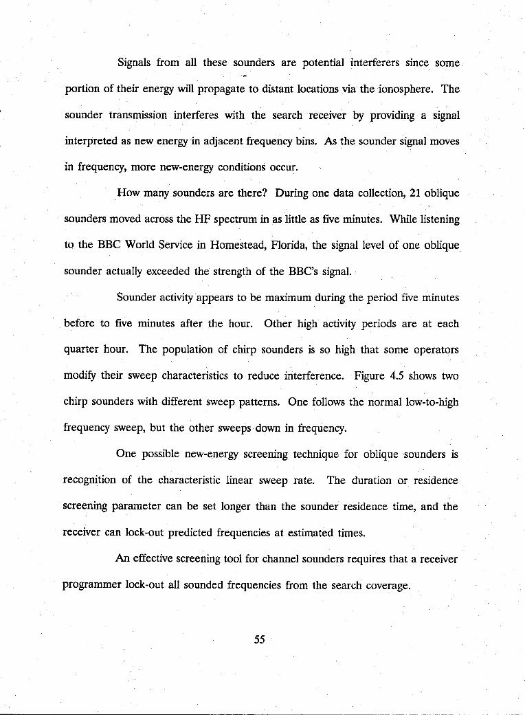
Signals from all these sounders are potential interferers since some

portion of their energy will propagate to distant locations via the ionosphere. The

sounder transmission interferes with the search receiver by providing a signal

interpreted as new energy in adjacent frequency bins. As the sounder signal moves

in frequency, more new-energy conditions occur.

How many sounders are there? During one data collection, 21 oblique

sounders moved across the HF spectrum in as little as five minutes. While listening

to the BBe World Service in Homestead, Florida, the signal level of one oblique

sounder actually exceeded the strength of the BBC's signal.

Sounder activity appears to be maximum during the period five minutes

before to five minutes after the hour. Other high activity periods are at each

quarter hour. The population of chirp sounders is so high that some operators

modify their sweep characteristics to reduce interference. Figure 4.5 shows two

chirp sounders with different sweep patterns. One follows the normallow-to-high

frequency sweep, but the other sweeps down in frequency.

One possible new-energy screening technique for oblique sounders is

recognition of the characteristic linear sweep rate. The duration or residence

screening parameter can be set longer than the sounder residence time, and the

receiver can lock-out predicted frequencies at estimated times.

An effective screening tool for channel sounders requires that a receiver

programmer lock-out all sounded frequencies from the search coverage.

55

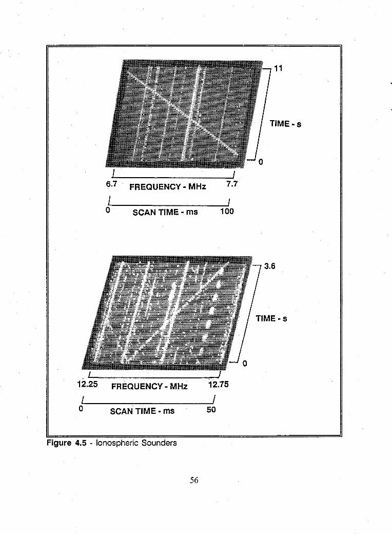
11

TIME - s

I 6.7 FREQUENCY _ MHz 7.7

I I o SCAN TIME - ms 100

3.6

. -

12.25 FREQUENCY - MHz 12.75

_1 ________ ~--------~1 o SCAN TIME· ms 50

Figure 4.5 - Ionospheric Sounders

56

5. Amplitude Keying

The most common form of HF amplitude modulation is the common

morse code transmission. Many morse code transmissions are signals of interest,

so search screening should not eliminate them. The on-off characteristic of the

signal will generate new-energy conditions, and the search process should recognize

the start of a morse code transmission.

To prevent continuous new-energy alarms, the signal decay time from

first new-energy detection should be longer than the spacing of slowly sent, manual

morse signals. This same process applies to any modulation type or transmission

profile which includes interrupted transmissions. However, a long decay parameter

may interfere with the detection of random frequency-hop signals. This is due to

the possibility of short frequency revisit times by the spread spectrum signal.

6. Spread-Spectrum Signals

Two frequency-hop spread-spectrum systems find use in the HF

spectrum. These are the coherent and non-coherent slow-frequency-hop regimes.

The second form is the more popular. HF slow-frequency-hop implies that the

residence time on one frequency exceeds the duration of one information bit [Ref.

30]. Observations of HF spread-spectrum transmissions find signals with residence

times exceeding 1 s.

The hopping spread is limited to a percentage of the maximum to

minimum propagation frequency range for the path of interest. The necessary

57

signal strength at the receiver site determines the percentage. In most cases, the

maximum frequency-hop range will be less than 1 MHz. Today's digital circuitry

makes it possible to use extremety long hopping patterns.

Each frequency transmitted generates a new-energy-present condition.

A single network of spread-spectrum, frequency-hopped stations could easily

inundate a new-energy receiver. Search receiver screening requires prior knowledge

of the specific hopping sequence and frequencies used.

B. HF NEW-ENERGY SURVEY

This author experimentally investigated the distribution of HF new-energy

events during the period 10 - 23 April 1989. The receiver site was the circularly

disposed antenna array, Wullenweber antenna, at Edzell, Scotland. The site is in

the single ionospheric hop footprint of all the major European international

broadcasting stations. Measurements during the period showed routine nighttime

maximum received signal strengths between 0 and -10 dBm. The strongest signals

were in the 49 and 31 meter international broadcast bands.

Because of the installation of an RF switching system, the new-energy survey

did not use the combined-omni antenna of the CDAA. Instead, a conical

monopole served as the omnidirectional search antenna.

1. System Description

Figure 4.6 is a block diagram of the search receiver system. The

receiver is a hybrid analog and digital system. The attenuation, frequency

58

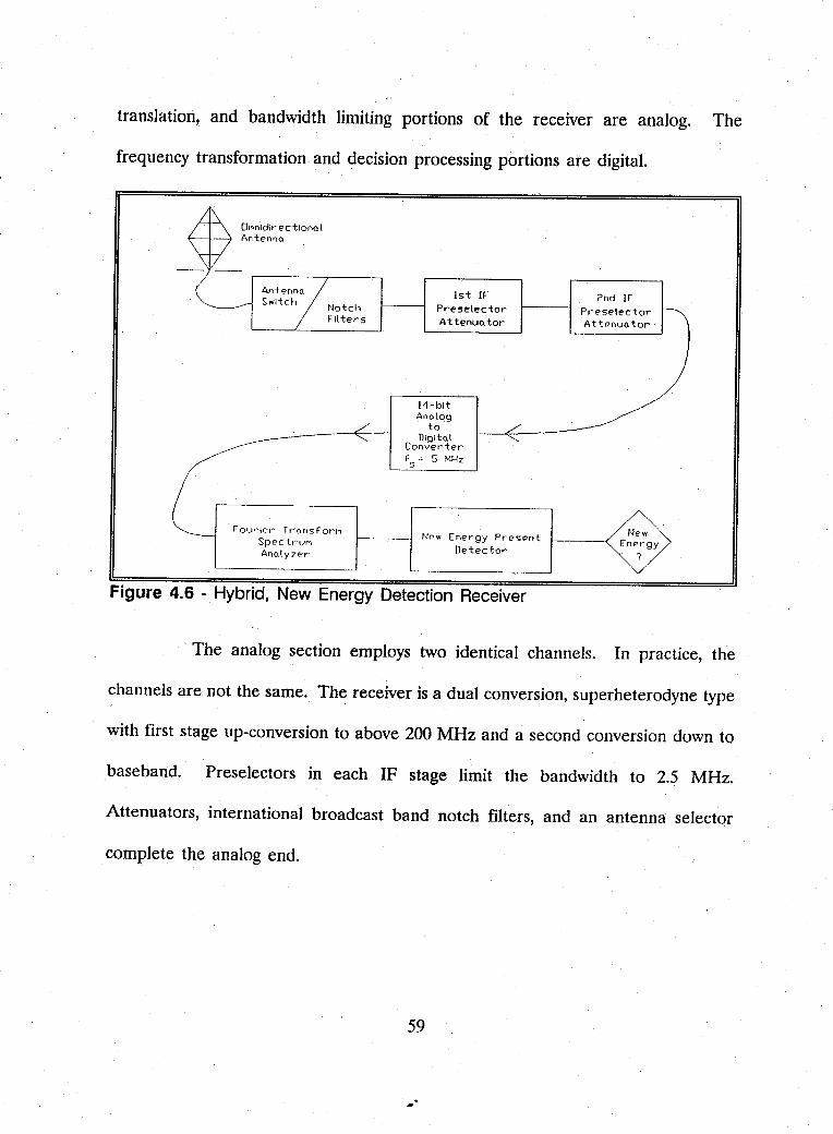
translation, and bandwidth limiting portions of the receiver are analog. The

frequency transformation and decision processing portions are digital.

O"nlclir eC tiona l An tenna

Ant'?nno SWitch Notch

Filters

rOut~ll?t'" Tt-onsforM SpectruM Analyzer

1st IF Preselector Attenuo tor

I4-blt Analog

to Digital

Converter r = 5 MHz s

New Energy Present Detecto,'

Figure 4.6 - Hybrid, New Energy Detection Receiver

2nd IF Preselector Attenuotor

New Energy

?

The analog section employs two identical channels. In practice, the

channels are not the same. The receiver is a dual conversion, superheterodyne type

with first stage up-conversion to above 200 MHz and a second conversion down to

baseband. Preselectors in each IF stage limit the bandwidth to 2.5 MHz.

Attenuators, international broadcast band notch filters, and an antenna selector

complete the analog end.

59

The key component in the receiver hardware is an Elsin 14-bit analog

to-digital converter operating at 5 MHz. The AID includes an integral sample

and-hold. The theoretical maximum dynamic range is 84 dB using the expression:

dynamic range in dB = 20n log10(2) ~ Sn (4.1)

where n is the number of bits of resolution in the analog-to-digital converter. The

actual dynamic range, by whatever measurement used, will always be less than the

theoretical value. A 12-bit Burr-Brown ADC-600 converter was also available as

an alternative NO device.

A single-tone measurement provided a 74 dB dynamic range for the

14-bit NO. Site personnel consistently measure a dynamic range in the mid

seventies for the Elsin converter. Single tone measurement provided a 66 to 68 dB

dynamic range for the Burr-Brown 12-bit converter.

The digital section includes a digital switching network, parallel Discrete

Fourier Transform spectrum analyzers, and new-energy-event detectors. The

Discrete Fourier Transform implementation is a Fast Fourier Transform algorithm

that includes a minimum 4-sample Blackman-Harris window. An overall process

controller manages detection identification, timing, control, and statistics. This

controller records each new~energy-present condition by time, center frequency, and

amplitude.

60

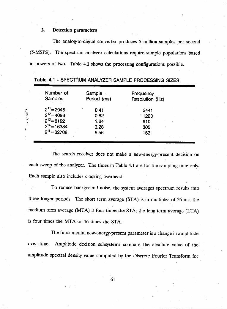
2. Detection parameters

The analog-to-digital converter produces 5 million samples per· second

(5-MSPS). The spectrum analyzer calculations require sample populations based

in powers of two. Table 4.1 shows the processing configurations possible.

Table 4.1 - SPECTRUM ANAL VZER SAMPLE PROCESSING SIZES

Number of Sample Frequency Samples Period (ms) Resolution (Hz)

Q 2"=2048 0.41 2441 Cl 2'2=4096 0.82 1220 l:;;

2'3=8192 1.64 610 . ~

., 2'4=16384 3.28 305 2':;=32768 6.56 153

The search receiver does not make a new-energy-present decision on

each sweep of the analyzer. The times in Table 4.1 are for the sampling time only.

Each sample also includes clocking overhead.

To reduce background noise, the system averages spectrum results into

three longer periods. The short term average (ST A) is in multiples of 26 ms; the

medium term average (MTA) is four times the STA; the long term average (LTA)

is four times the MTA or 16 times the STA.

The fundamental new-energy-present parameter is a change in amplitude

over time. Amplitude decision subsystems compare the absolute value of the

amplitude spectral density value computed by the Discrete Fourier Transform for

61

each frequency bin. As described in part A above, there are many potential

energies that are not of interest to the search process that the amplitude parameter

screening alone will not adequately eliminate. Amplitude screening by the search

receiver produces a first subset of the new energies present. To improve the

probability that the new energy is a signal of interest, additional parameter

screening is necessary. The two additional screening parameters are time and

bandwidth.

The time screening process requires that the new energy be present for

a programmable number of ST A's. Otherwise, it is not of interest. The time

parameter also screens repetitive new energies such as those from amplitude shift

keying or pulsed noise. Once a new energy disappears for at least one STA, the

receiver allows energy in that bin to decay. During the decay period of one LTA,

the receiver assumes that an amplitude change exceeding the new-energy threshold

in the same bin to be from the same source as the previous new energy.

The bandwidth screening process assumes that all signals of interest (i.e.,

communications signals) are bandwidth limited. This should screen out new

energies from lightning and impulsive noise which typically are several megahertz

wide. The bandwidth window must be large enough for data communications

using multiple tones and data rates as high as 1200 BAUD. Another bandwidth

screening requires a minimum bandwidth to reduce noise effects.

62

3. Data Collection

The data collection included a series of 34 individual sets ranging in time

duration from 15 minutes to 14~ hours. Data file oversize errors in the system

control processor resulted in losing four data sets before accomplishing histogram

processing, and the failure of one NO converter resulted in losing another data

set. In the remaining 29 data sets, 4,317,021 total new-energy-present conditions

were obtained. The largest collection period had 1,373,554 new energies, and the

smallest collection period had 1236 new energies. The receiver created a log of

each new-energy event.

The data collection used both NO channels, separate spectrum

analyzers, and separate detectors. In all cases, the same analog receiver portion

fed both NO's. The sets included daytime, transition, and nighttime periods.

Most sets used an 8 dB amplitude detection threshold level. A new

energy may be present when the ST A amplitude calculated for a given frequency

bin exceeds the amplitude level calculated in the last LTA for the same frequency

bin by an amount greater than the amplitude detection threshold level.

Data sets 1 through 7 used a single 14-bit NO converter. Sets 8

through 18 (daytime) and sets 19 through 26 (nighttime) used a 14-bit NO on one

channel and a 12-bit NO on the parallel channel. Sets 8 through 26 employed the

different word size NO's provided data to compare dynamic range and saturation

effects. Sets 27 through 34 utilized two 14-bit NO's. Tests 32 through 34 used an

63

8 dB amplitude detection threshold on one channel and a· 16 dB threshold on the

parallel channel. Data sets 3, 10, 27, 28, and 29 were lost.

In general, data set collection used the minimum preselector/lF stage

attenuation needed to prevent NO overload. The data sets comparing the

different word-length NO's varied the attenuation from test to test. The best

indicator of NO overload was a sudden jump in the new-energy activity.

To reduce the data, the control processor produced an amplitude

histogram for each data set from the new-energy-event log. The amplitude value

used in histogram production for each new energy was the maximum amplitude

spectral density value calculated for the MT A associated with that event. The

control processor also produced amplitude histograms of the new energies unique

to each channel and of new energies common to both channels. The control

processor performed all data reduction off-line.

4. Histogram Results

Figure 4.7 shows the histogram for data identified as set 34. Appendix

B contains histogram presentations of the data obtained for the remaining sets.

The shape of the probability density functions in the dBm domain

suggest a log.:.normal distribution of the received voltage amplitude. Following this

assumption, the dB-domain normal distribution estimation of mean and variance

were calculated using the three techniques described in Chapter III.

64

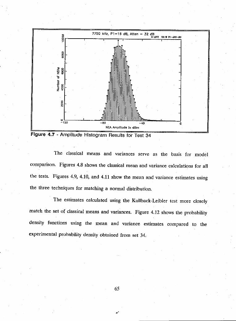
g 7750 kHz, P1 == 16 dB, Atten = 32 dB o LOTT 10;111 :ll-JA,'I-1I0

g~----~------~--~~-------r------r------'

... o .. .,

§ ID

.a 0 E 0 :::I 0 Z ....

o o ~

-

---

o L-~-"TiLJ.Wl.l.l.llllllLJ.Wl.l.l.lllll~~-----.I--120 -BO -oH) 0

NEA Amplitude In dBm

Figure 4.7 - Amplitude Histogram Results for Test 34

The classical means and variances serve as the basis for model

comparison. Figures 4.8 shows the classical mean and variance calculations for all

the tests. Figures 4.9, 4.10, and 4.11 show the mean and variance estimates using

the three techniques for matching a normal distribution.

The estimates calculated using the Kullback-Leibler test more closely

match the set of classical means and variances. Figure 4.12 shows the probability

density functions using the mean and variance estimates compared to the

experimental probability density obtained from set 34.

65

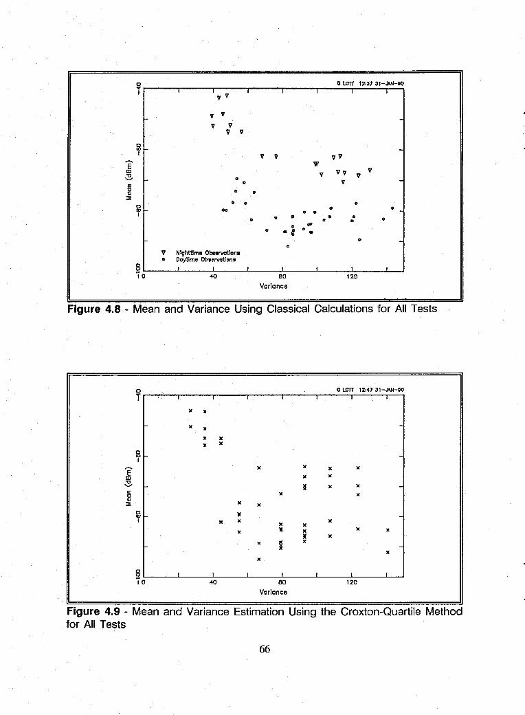
0 o l.C1T 12:37 Jl-JAN-gO

T V V

I I I I I

V V

V V V v

0 to I V V VV ......

VI E aJ

V Vv V 'll V ........ 0

c 0 V c 0 0 CII

::::;; 0 0 0

0 • 0

'" 00 0 0 I 0 D 0 0

0 0 0 0

0 <P 0 • « 0 •

0

0

V Nlghttlma Obaflrvctlona 0 Daytime Observations

c 0

'10 040 80 120

Variance

Figure 4.8 - Mean and Variance Using Classical Calculations for All Tests

0 o l.C1T 12:47 3'-JAN-DO

T I I

)( X

X X

X )(

X IC

0 ID I

E IC )( IC )(

aJ IC IC 'll ....... l! IC )(

c: )( )( c ., ::::;; IC )(

0 ,. -'" I )( )( )(

)( )(

)( .. )( )( x

II )(

)( B )(

x )(

c I 1 1 I 1 I I 0

'10 040 80 120

Variance

Figure 4.9 - Mean and Variance Estimation Using the Croxton-Quartile Method for All Tests

66

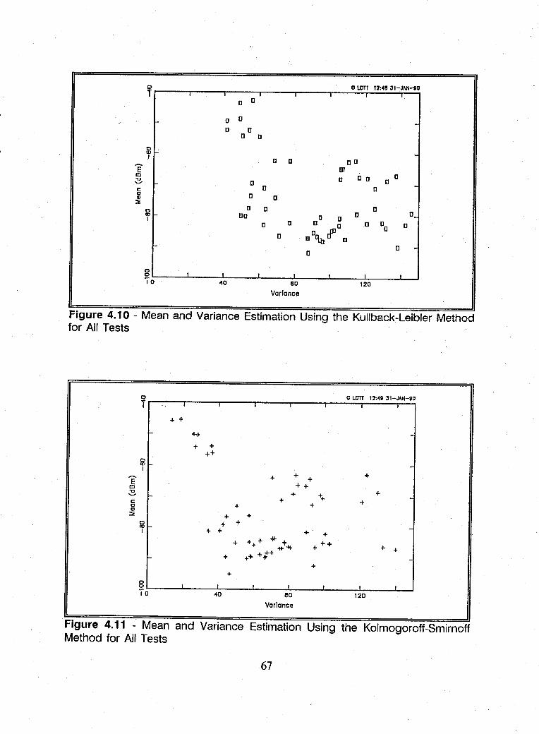
o I.D1T 12:~1I 31-JAN-OO I I Il I

I

[]

Il [] -[] Il

Il []

0 w -I [] [] DD

E IJI m [] D D Il v [] ...... f0- Il e D [] c [] [] .. :l:

IE: I-D [] []

[] IlD [] D

I [] [] [] o D 0 [] []

o,tP ° []

[]

[] []

0 _I 0 I I I I I I 10 "10 eo 120

Variance

Figure 4.10 - Mean and Variance Estimation Using the Kullback-Leibler Method for All Tests

E m '"0 ...... e c .. ::::

o 0 I.D1T 12:~9 Jl-JAN-SO T~~~----~----~--~-----r----~----o-I~

+ + I- ++

0 'fI-

l-

0 'fl-

f-

0 0

10

+ + ++

+ + +

+ + + +

+

+ + + + +

+ +

eo Variance

+

+ +

+ ++

+

+

+ +

+ +

I

120

Figure 4.11 - Mean and Variance Estimation Using the Kolmogoroff-Smirnoff Method for All Tests

67

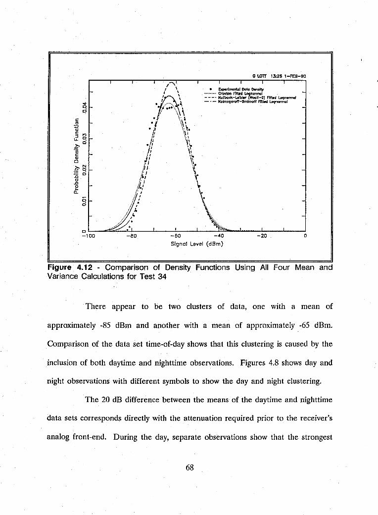
~ o c:i

o d

G LOTT 13:26 l-FEB-90

• "-rlm.ntal Data Don.1ty .......... CroxI<>n ntt.d lDvnormal - - -. Kullbod<-LAlblo, (Woolf-G) ntt.d lo9normal - • - Koimogorvff-Smlmotf F1tt~ lo9'1Om1QI

oL-__ ~~~~ __ _L ____ ~ __ ~ ____ ~~~ ____ ~ __ ~ ____ ~

-100 -80 -60 -40

Signol Level (dBm)

-20 o

Figure 4.12 - Comparison of Density Functions Using All Four Mean and Variance Calculations for Test 34

There appear to be two clusters of data, one with a mean of

approximately -85 dBm and another with a mean of approximately -65 dBm.

Comparison of the data set time-of-day shows that this clustering is caused by the

inclusion of both daytime and nighttime observations. Figures 4.8 shows day and

night observations with different symbols to show the day and night clustering.

The 20 dB difference between the means of the daytime and nighttime

data sets corresponds directly with the attenuation required prior to the receiver's

analog front-end. During the day, separate observations show that the strongest

68

signals were in the 19 and 17 meter international broadcast bands with peak levels

of -30 dBm. With the receiver dynamic range near 75 dB and without front-end

attenuation, distortion products would appear in the receiver if the receiver's

sensitivity was kept at the measured minimum sensitivity of -116 dBm. Thus

daytime receiver operation required 12 to 28 dB of front-end attenuation to prevent

the generation of distortion products.

At night, the strongest signals were in the 31 and 49 meter international

broadcast band with peak signal levels of 0 dBm. Nighttime receiver operation

required 36 to 54 dB of front-end attenuation to prevent distortion products.

Routine receiver operation proves that there is a 20 to 30 dB difference in receiver

front-end attenuation requirements between day and night operation.

The limited receiver dynamic range and the resulting receiver front-end

attenuation requirements prevents detection of the weakest signals. One can see

the result of lost receiver sensitivity in the sharp rise on the weaker signal side of

the experimental density functions. The weaker signals are there, but they are not

detectable by the system.

Even with this skew in the low end of the experimental density functions,

the log-normal assumption appears valid. In fact the less-steep weaker signal slope

of the theoretical densities fitted using the estimation techniques may more

accurately represent the true signal population. The less-steep slope would come

from a distribution with a larger variance.

69

An important point is that the distributions represent the population of

signals detectable by the receiver. Ideally, signals exist far below kTB noise levels,

but they are not detectable. The new-energy-survey distributions are for signals

which exceed the ambient noise levels by the specified amplitude threshold.

c. SUMMARY OF RESULTS

The log-normal signal amplitude distribution is a good model for new-energy

present conditions. This model matches the results from the overall HF signal

amplitude or channel occupancy surveys discussed in Chapter III. Figure 4.13

shows two theoretical signal amplitude probability distribution functions generated

using daytime and nighttime new-energy-detection data. Figure 4.14 shows the two

corresponding density functions.

General HF spectrum surveys, excluding international broadcasting, are valid

predictors of new-energy levels. There appears to be little signal population

difference between weekdays and weekends.

The shift in the mean signal level from day to night is significant enough to

warrant using different day and night system design criteria. The nighttime signal

population establishes the dynamic range requirements for the search system

excluding international broadcasting signals. Design should always incorporate the

best receiver sensitivity possible with practical values near -125 dBm. The new

energy signals alone require a receiver dynamic range of 85 dB (from -125 to -40

dBm). However, the overall dynamic range requirement (as shown in Chapters 2

70

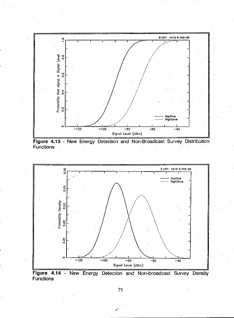
G LOTI 14:13 8-FEB-tO ~r----r----~--~----~--~----~---'----.-~~----, ..........................

1i a:J > ' 3 0

c c: 01

Vi ID .., d C c: 01

'iii .... o ..,. :5 d

g :0 c .c o N

D: 0

... .... :'

.r' ./ ,

" i

. '

/ :'

/ f

l /'

:/ !

" ... ~// _.- Daytime ............ Nighttime

o~--~--~~--~~~~--~ __ --~--~ ____ ~ __ ~ ____ ~ -120 -80 -60 -40

Signal Level (dBrn)

Figure 4.13 - New Energy Detection and Non-Broadcast Survey Distribution Functions

gr-__ -r ____ r-__ -r ____ ~--~----~--~--~C~LOTI~~1~4:~18~6~-~FE~D-~9~O

<of o d

o d

-- Oaytlmll ............ Nlghlllmll

//"."." .. \\ ! \

: .. ,

\., .. . ,/' "

.1 \ "

f \ . ...

................... . ................ . O~--~~--L--=~~ __ ~ __ ~~ __ ~~~ ____ ~ __ ~~ __ J

-120 -40

Signal Level (dBrn)

Figure 4.14 - New Energy Detection and Npn-broadcast Survey Density Functions

71

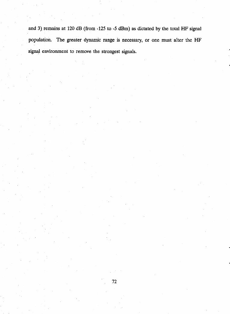
and 3) remains at 120 dB (from -125 to -5 dBm) as dictated by the total HF signal

population. The greater dynamic range is necessary, or one must alter the HF

signal environment to remove the strongest signals.

72

v. HF SITE PERFORMANCE CRITERIA

The distributions of standard HF signals and new signal energies provide a

basis to determine a site's ability to receive signals of interest. From distributions

of signal strengths, one can determine the effects of noise and signal attenuation

on the reception of signals of interest. Noise and signal path attenuation have

predictable and harmful effects on signal reception.

Signal attenuation and noise levels can be related to the percentage of signals

of interest lost. The signals of interest are usually the clandestine transmitters,

weak mobile transmitters, and stations using low power transmitters and inefficient

antennas. The search function rarely looks for international broadcast band signals.

Because of the search target characteristics, a signal distribution used to

measure site performance is misleading if it includes international broadcast

stations. However, the overall signal handling capability of the search receiver must

include these strong signals.

Site performance quantification began with the Navy's Signal-to-Noise

Enhancement Program (SNEP). Researchers at the Naval Postgraduate School

observed harmful interference at various HF receiver sites. Lead by Professors

Steve Jauregui and W. Ray Vincent, site noise surveys found many signals of

interest being obscured by various noise sources.

73

There are many Department of Defense programs to reduce interference

effects. These typically fall under the category of electromagnetic interference/radio

frequency interference (EMI/RFI). Noise and interference, from whatever the

source, reduces a receiver site's ability to perform its mission. Yet, rarely do

EMI/RFI programs try to quantify a level of degradation in signals or targets lost.

EMI/RFI programs do nothing to mitigate the signal path attenuation effects.

These programs tend to emphasize "noise reduction" rather than overall site

performance improvement.

SNEP research revealed that there is another, equally important side to site

performance improvement. Surveys found there is a baseline noise level within

the radio frequency path from antenna to receiver at almost all Navy CDAA sites.

This noise is the composite of externally and internally generated sources, and it

is present at all receivers in the facility. A typical figure is -120 dBm in a 3 kHz

bandwidth.

This noise level is present regardless of the signal attenuation characteristics

within the RF signal path. This noise floor is rarely below -125 dBm in a 3 kHz

bandwidth. The noise baseline varies with time-of-day, season, frequency, etc. The

variable noise level is always stronger than the baseline level. The instantaneous

value of the noise masks signals-of-interest. A long term average cannot truly

represent the base noise value.

74

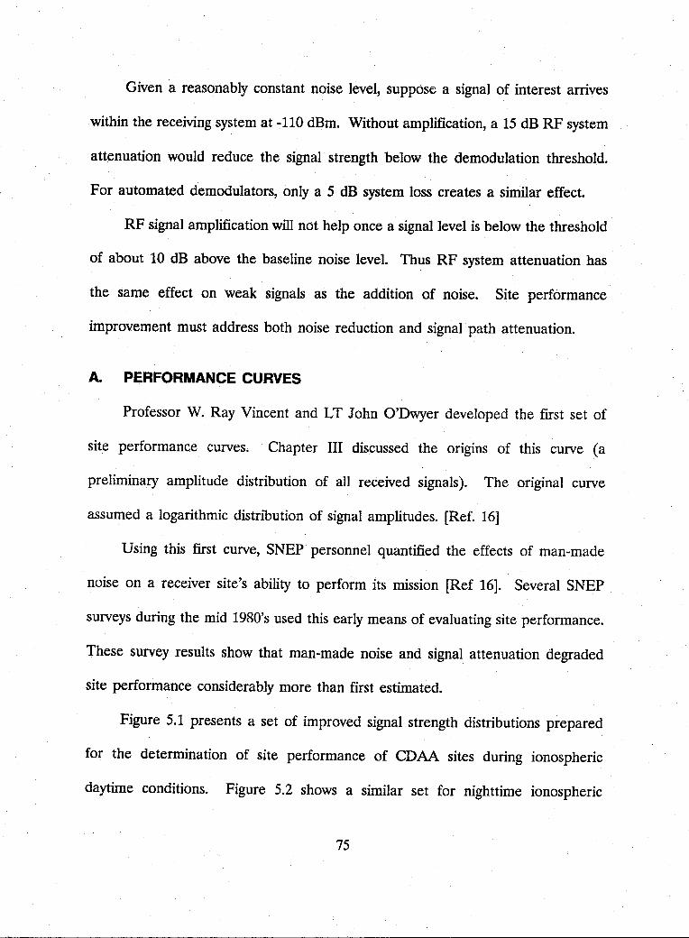
Given a reasonably constant noise level, suppose a signal of interest arrives

within the receiving system at -110 dBm. Without amplification, a 15 dB RF system

attenuation would reduce the signal strength below the demodulation threshold.

For automated demodulators, only a 5 dB system loss creates a similar effect.

RF signal amplification will not help once a signal level is below the threshold

of about 10 dB above the baseline noise level. Thus RF system attenuation has

the same effect on weak signals as the addition of noise. Site performance

improvement must address both noise reduction and signal path attenuation.

A. PERFORMANCE CURVES

Professor W. Ray Vincent and LT John O'Dwyer developed the first set of

site performance curves. Chapter III discussed the origins of this curve (a

preliminary amplitude distribution of all received signals). The original curve

assumed a logarithmic distribution of signal amplitudes. [Ref. 16]

Using this first curve, SNEP personnel quantified the effects of man-made

noise on a receiver site's ability to perform its mission [Ref 16]. Several SNEP

surveys during the mid 1980's used this early means of evaluating site performance.

These survey results show that man-made noise and signal attenuation degraded

site performance considerably more than first estimated.

Figure 5.1 presents a set of improved signal strength distributions prepared

for the determination of site performance of CDAA sites during ionospheric

daytime conditions. Figure 5.2 shows a similar set for nighttime ionospheric

75

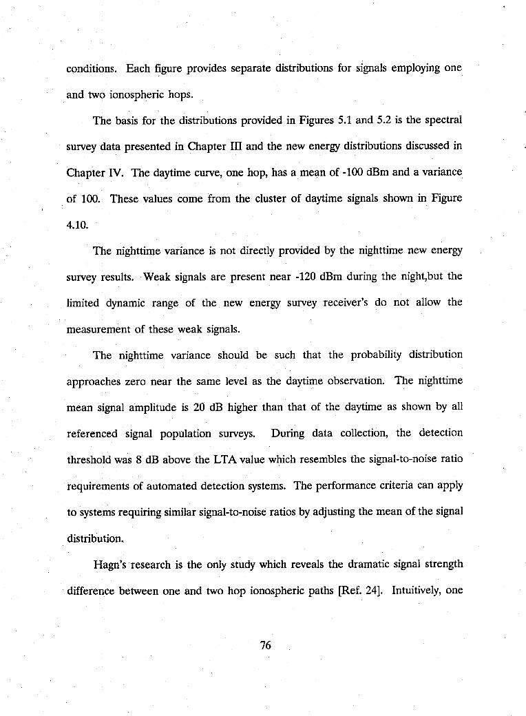
conditions. Each figure provides separate distributions for signals employing one

and two ionospheric hops.

The basis for the distributions provided in Figures 5.1 and 5.2 is the spectral

survey data presented in Chapter III and the new energy distributions discussed in

Chapter N. The daytime curve, one hop, has a mean of -100 dBm and a variance

of 100. These values come from the cluster of daytime signals shown in Figure

4.10.

The nighttime variance is not directly provided by the nighttime new energy

survey results. Weak signals are present near -120 dBm during the night,but the

limited dynamic range of the new energy survey receiver's do not allow the

measurement of these weak signals.

The nighttime variance should be such that the probability distribution

approaches zero near the same level as the daytime observation. The nighttime

mean signal amplitude is 20 dB higher than that of the daytime as shown by all

referenced signal population surveys. During data collection, the detection

threshold was 8 dB above the LTA value which resembles the signal-to-noise ratio

requirements of automated detection systems. The performance criteria can apply

to systems requiring similar signal-to-noise ratios by adjusting the mean of the signal

distribution.

Hagn's research is the only study which reveals the dramatic signal strength

difference between one and two hop ionospheric paths [Ref. 24]. Intuitively, one

76

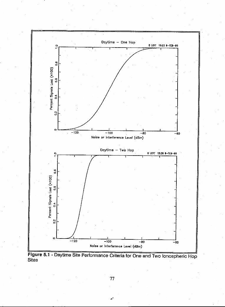
0' 0 ..-)( ........ .... III

.3

.!'l D t: 01 iii .... t: OJ U "-OJ Il.

0' 0

)( ........ .... III

.3 ., C t:

.2' III .... t:

tl "-OJ Il.

Daytime - One Hop C LC1TT 11l,2J IS-FEB-eO

~r------'r------'-------.-------.------~~=----r------~

IX)

d

CD d

"": 0

N d

I I I I I I I I

I I I I I I I I I I ..

o~--~~~----~------~------~------~------~------~ . -120 -100 -80 -60

Noise or Interference Level (dBm)

Daytime - Two Hop C um 11l:2!J a-FEB-eO

~r------'r------'~-----.-------.------~-------r------~

I I I

ID d

I CD d

..t-d

N d

I I I I

o~--~~~----~------~------~------~------~------~ -120 -100 -80 -60


Figure 5.1 - Daytime Site Performance Criteria for One and Two Ionospheric Hop Sites

77

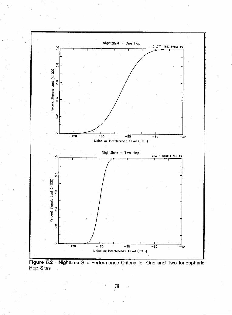
Nighttime - One Hop ~r-__ -'r-__ -.,-__ -, ____ -. ____ -. ____ ~ ____ ~G~lorr~~1~8:~27~8~-~IT=B~-'~O

III o

OL---~~~~~ __ ~~ __ ~ ____ ~ ____ ~ ____ ~ ____ -L ____ ~ -80 -60 -40


Nighttime - Two Hop o G lorr 115:215 IS-ITB-DO ~r-----r----.r----'----~----~----~-----r-----r----~

10 0

0' 0 .... )( '-" - CO III 0 0 --l

III 0 t:

.2' .t (IJ 0 .... c

B ... tl

0.

~

OL-__ ~~ ____ ~ __ ~ ____ ~ ____ ~ ____ ~ ____ ~ ____ _L ____ ~

-100 -BO -60 -40 Noise or Interference Level (dBm)

Figure 5.2 - Nighttime Site Performance Criteria for One and Two Ionospheric Hop Sites

78

would expect the two-hop signal to be weaker. The strongest two-hop signals

should be from international broadcast stations. Even in the two-hop signal case,

the weakest detectable signal must have a power level well above the instantaneous

noise floor during the measurement. These characteristics of two-hop signals result

in a lower mean, but the greatest effect is a smaller variance which is shown by an

increased slope of the performance curve. For example, if signal path conditions

result in increased signal levels, a two-hop site will hear relatively more signals than

a one hop site.

B. ESTIMATING PERFORMANCE FROM SITE MEASUREMENTS

There are five steps necessary to assess HF receiver site performance. These

are:

+ Determine the distance to typical transmitters-of-interest and international broadcasters and establish the resulting number of ionospheric hops.

+- Determine the strongest signals received.

+ Determine internally caused baseline noise levels as seen at a receiver.

+ Determine external noise levels and other factors which further degrade site performance.

+ Determine the RF distribution system signal attenuation.

1. Distance and Ionospheric Path

There are two signal path distances one must determine as the first step

to assess receiver site performance. One distance helps determine the maximum

signal strength of signals from international broadcasting stations to establish the

79

total system dynamic range requirements. The other distance determines which set

of performance curves to use.

The distance to international broadcasting stations requires identification

of those broadcasters which target the area where the receiver is situated. A

receiver site in Guam falls in the Northern Pacific Islands target area or the

broader Far East, Pacific, or Oceania target areas. The current edition of the

World Radio Television Handbook is an excellent guide for locating the international

broadcast station locations.

The Voice of America schedules transmissions to "Oceania" using relay

stations in the Philippines, Sri Lanka, and Thailand. The U.S.S.R. State Committee

for Television and Radio Broadcasting (Radio Moscow) extensively targets the

South East Asian and Pacific areas for HF coverage. Transmitter sites used for this

coverage include Chita (Aleksandrovka), Pettropavlovsk-Kamchatskiy, and

Vladivostok. The Australian Broadcasting Corporation (Radio Australia) uses

transmitters located in Darwin, Shepparton, and Carnarvon to beam programs to

East Asia, Northern Pacific Islands, and Paupa/New Guinea. Signals from all these

(and many other broadcast stations) are the strongest signals received at the

receiver site on Guam. [Ref. 3]

The distance from Guam to these sites is typically one ionospheric hop.

However, the major target areas for broadcasts to this region are the Philippines

and Indonesia. This is due to the population densities and the political situations

80

in the region. So Guam is on the periphery of the coverages. While signals will

be single hop, the actual signal strengths should not be exceedingly high because

of transmitting antenna beam effects. One could expect the strongest signals to be

broadcasts targeted for evening reception in the 31, 41 and 49 meter bands [Ref.

3].

Three field techniques are available to determine the path distances.

One is to take an inexpensive world globe available in most book stores. By using

a string, one can mark off distances between broadcast transmitters and a receiver

site along great circles centered on the receiver facility. This method provides an

excellent pictorial representation for operational personnel.

The second is to use one of the many ray tracing programs available for

small computers. There are several programs used by amateur radio operators that

can provide bearing and distance between specified points. By entering the location

of suspected transmitters-of-interest, the program can calculate the distances and

display the path on a map.

A third field technique is to use the PROPHET program developed by

the Naval Ocean System Center, San Diego. The specific program in PROPHET

Ver. 3.2 is Raytrace. This can provide not only distances, but it can determine if

the path is most likely one or two ionospheric hop. PROPHET can provide many

other estimates of path conditions. [Ref. 31]

81

2. Strongest Signal Measurements

To establish the strongest signals present at a receiver site, one must

measure the signal strengths at three locations. These are the antenna elements,

the outputs of the RF distribution system, and the antenna input terminal of a

typical HF receiver used in the facility.

During a visit to the Guam CDAA facility in September 1989, the SNEP

team investigated the potential interference from two international shortwave

broadcasting stations located on the island. KTWR, located near the town of

Merizo, uses four 100 kw transmitters and two large curtain array antennas.

Program target areas are China and South East Asia. KSDA, located near the

town of Agat, uses two 100 kw transmitters and two curtain arrays also beamed

towards South East Asia. Both transmitter sites are on the southwest end of

Guam. This is some 15 miles from the receiver site located in the northwest corner

of the island.

There are also two international broadcasting stations located on the

island of Saipan approximately 300 miles from the Guam receiver site. KFBS near

Marpi uses three 100 kw transmitters, and KYOI at Agingan Point uses one 100

kw transmitter. [Ref. 3]

This author monitored transmissions from these broadcasters throughout

their broadcast schedules. The signals received at the CDAA were not any stronger

than the average international broadcast signal received by ionospheric modes. The

82

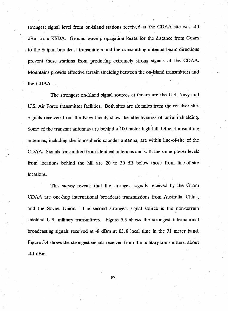
strongest signal level from on-island stations received at the CDAA site was -40

dBm from KSDA. Ground wave propagation losses for the distance from Guam

to the Saipan broadcast· transmitters and the transmitting antenna beam directions

prevent these stations from producing extremely strong signals at the CDAA.

Mountains provide effective terrain shielding between the on-island transmitters and

the CDAA.

The strongest on-island signal sources at Guam are the U.S. Navy and

U.S. Air Force transmitter facilities. Both sites are six miles from the receiver site.

Signals received from the Navy facility show the effectiveness of terrain Shielding.

Some of the transmit antennas are behind a 100 meter high hill. Other transmitting

antennas, including the ionospheric sounder antenna, are within line-of-site of the

CDAA. Signals transmitted from identical antennas and with the same power levels

from locations behind the hill are 20 to 30 dB below those from line-of-site

locations.

This survey reveals that the strongest signals received by the Guam

CDAA are one-hop international broadcast transmissions from Australia, China,

and the Soviet Union. The second strongest signal source is the non-terrain

shielded U.S. military transmitters. Figure 5.3 shows the strongest international

broadcasting signals received at -8 dBm at 0318 local time in the 31 meter band.

Figure 5.4 shows the strongest signals received from the military transmitters, about

-40 dBm.

83

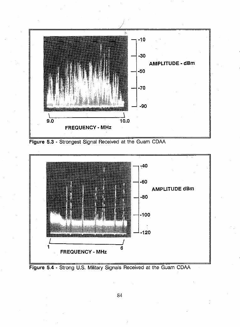
AMPLITUDE - dBm·

\ \ 9.0 10.0

FREQUENCY - MHz

Figure 5.3 - Strongest Signal Received at the Guam COM

~40

-60

AMPLITUDEdBm

-80

-100

-120 ~L ______________ ~I

1 6 FREQUENCY - MHz

Figure 5.4 - Strong U.S. Military Signals Received at the Guam COM

84

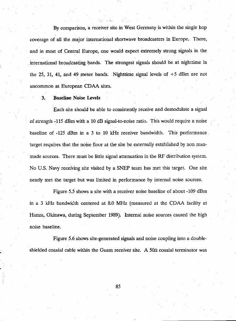
By comparison, a receiver site in West Germany is within the single hop

coverage of all the major international shortwave broadcasters in Europe. There,

and in most of Central Europe, one would expect extremely strong signals in the

international broadcasting bands. The strongest signals should be at nighttime in

the 25, 31, 41, and 49 meter bands. Nighttime signal levels of +5 dBm are not

uncommon at European CDAA sites.

3. Baseline Noise Levels·

Each site should be able to consistently receive and demodulate a signal

of strength -115 dBm with a 10 dB signal-to-noise ratio. This would require a noise

baseline of -125 dBm in a 3 to 10 kHz receiver bandwidth. This performance

target requires that the noise floor at the site be externally established by non man

made sources. There must be little signal attenuation in the RF distribution system.

No U.S. Navy receiving site visited by a SNEP team has met this target. One site

nearly met the target but was limited in performance by internal noise sources.

Figure 5.5 shows a site with a receiver noise baseline of about -109 dBm

in a 3 kHz bandwidth centered at 8.0 MHz (measured at the CDAA facility at

Hanza, Okinawa, during September 1989). Internal noise sources caused the high

noise baseline.

Figure 5.6 shows site-generated signals and noise coupling into a double

shielded coaxial cable within the Guam receiver site. A 50n coaxial terminator was

85

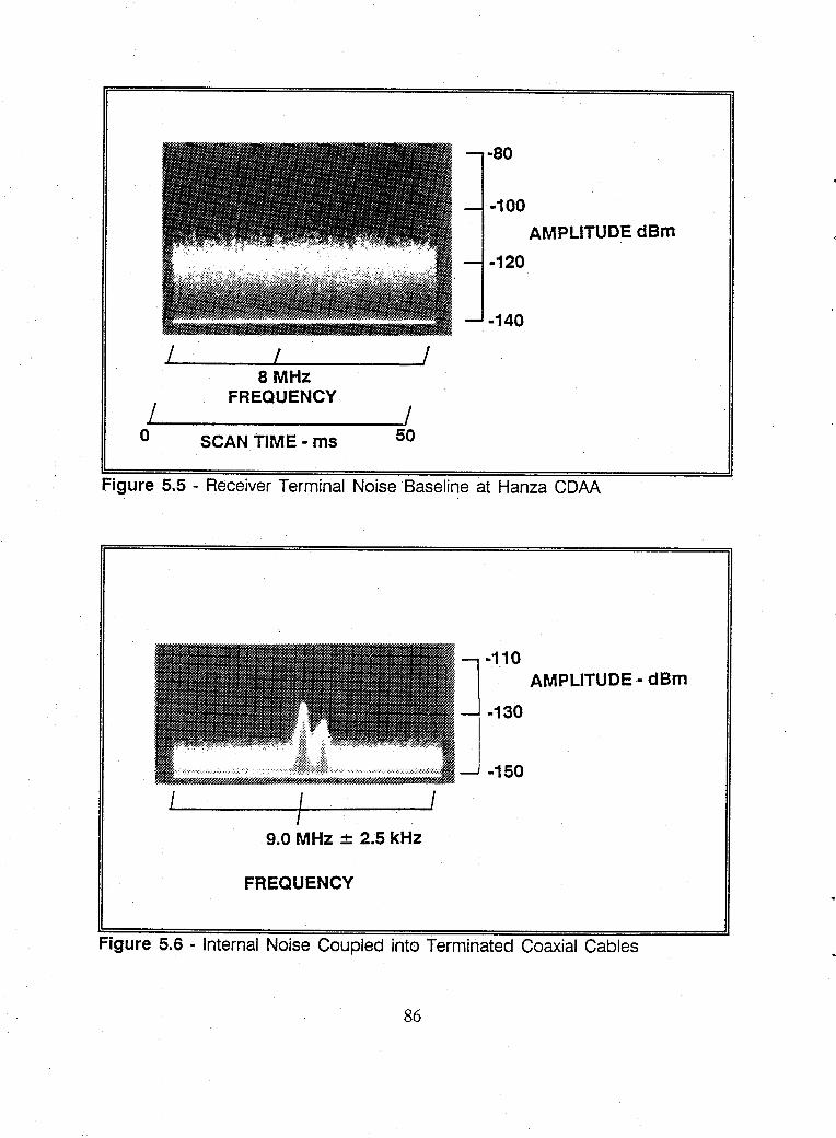
~/ ______ ~I ________ ~1 8MHz

FREQUENCY ~/--------------~/

o SCAN TIME - ms 50

-100

AMPLITUDE dBm

-120

-140

Figure 5.5 - Receiver Terminal Noise Baseline at Hanza COM

-110 AMPLITUDE - dBm

-130

-150

I , I

9.0 MHz ± 2.5 kHz

FREQUENCY

Figure 5.6 - Internal Noise Coupled into Terminated Coaxial Cables

86

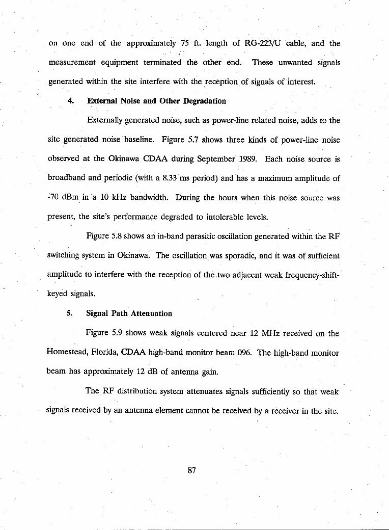
on one end of the approximately 75 ft. length of RG-2231U cable, and the

measurement equipment terminated the other end. These unwanted signals

generated within the site interfere with the reception of signals of interest.

4. External Noise and Other Degradation

Externally generated noise, such as power-line related noise, adds to the

site generated noise· baseline. Figure 5.7 shows three kinds of power-line noise

observed at the Okinawa CDAA during September 1989. Each noise source is

broadband and periodic (with a 8.33 ms period) and has a maximum amplitude of

-70 dBm in a 10 kHz bandwidth. During the hours when this noise source was

present, the site's performance degraded to intolerable levels.

Figure 5.8 shows an in-band parasitic oscillation generated within the RF

switching system in Okinawa. The oscillation was sporadic, and it was of sufficient

amplitude to interfere with the reception of the two adjacent weak frequency-shift

keyed signals.

5. Signal Path Attenuation

Figure 5.9 shows weak signals centered near 12 MHz received on the

Homestead, Florida, CDAA high-band monitor beam 096. The high-band monitor

beam has approximately 12 dB of antenna gain.

The RF distribution system attenuates signals sufficiently so that weak

signals received by an antenna element cannot be received by a receiver in the site.

87

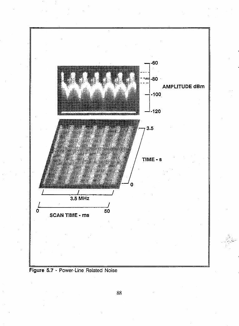
~/--------~/------~I 3,5 MHz

~/----------------~I o 50 SCAN TIME - ms

Figure 5,7 - Power-Line Related Noise

88

-60

AMPLITUDEdBm

-100

-120

3,5

TIME - s

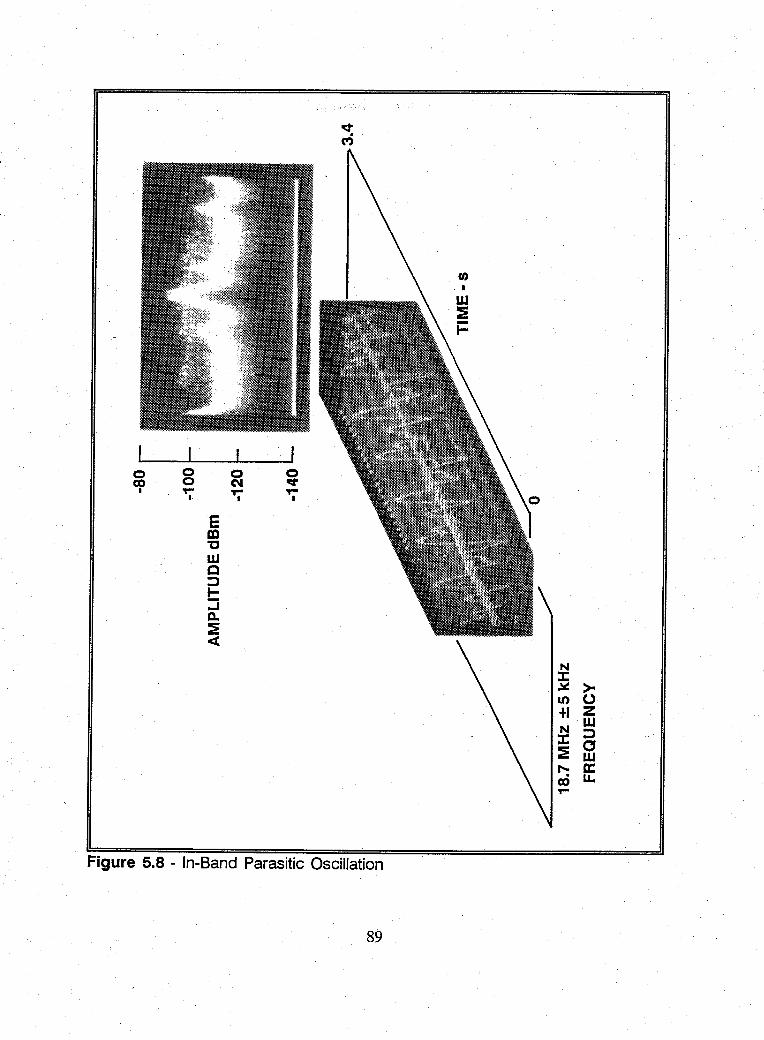
0 0 0 0 CO 0 C\I ~

I ,.. ,.. ,.. I, I I

E m 'C w c :::> I-::l D. :E «

N :t: ~ > It) 0 +1 Z N

W :::> :t:

" :E w ...... a: cO u. ,..

Figure 5.8 - In-Band Parasitic Oscillation

89

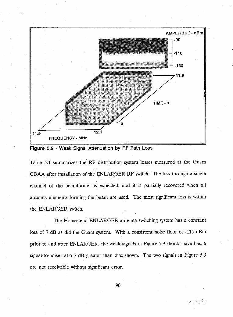
AMPLITUDE-dBm

·90

·110

·130

-----,11.9

TIME-s

11.9 12.1 FREQUENCY· MHz

Figure 5.9 - Weak Signal Attenuation by RF Path Loss

Table 5.1 summarizes the RF distribution system losses measured at the Guam

CDAA after installation of the ENlARGER RF switch. The loss through a single

channel of the beamformer is expected, and it is partially recovered when all

antenna elements forming the beam are used. The most significant loss is within

the ENLARGER switch.

The Homestead ENlARGER antenna switching system has a constant

loss of 7 dB as did the Guam system. With a consistent noise floor of -115 dBm

prior to and after ENLARGER, the weak signals in Figure 5.9 should have had a

signal-to-noise ratio 7 dB greater than that shown. The two signals in Figure 5.9

are not receivable without significant error.

90

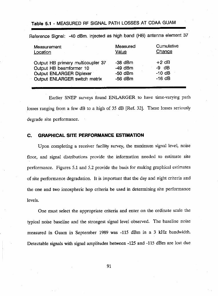
Table 5.1 - MEASURED RF SIGNAL PATH LOSSES AT CDAA GUAM

Reference Signal: -40 dBm. injected as high band (HB) antenna element 37

Measurement Location

Output HB primary multicoupler 37 Output HB beamformer 10 Output ENLARGER Diplexer Output ENLARGER switch matrix

Measured Value

-38 dBm -49 dBm -50 dBm -56 dBm

Cumulative Change

+2 dB -9 dB -10 dB -16 dB

Earlier SNEP surveys found ENLARGER to have time-varying path

losses ranging from a few dB to a high of 35 dB [Ref. 32]. These losses seriously

degrade site performance.

C. GRAPHICAL SITE PERFORMANCE ESTIMATION

Upon completing a receiver facility survey, the maximum signal level, noise

floor, and signal distributions provide the information needed to estimate site

performance. Figures 5.1 and 5.2 provide the basis for making graphical estimates

of site performance degradation. It is important that the day and night criteria and

the one and two ionospheric hop criteria be used in determining site performance

levels.

One must select the appropriate criteria and enter on the ordinate scale the

typical noise baseline and the strongest signal level observed. The baseline noise

measured in Guam in September 1989 was -115 dBm in a 3 kHz bandwidth.

Detectable signals with signal amplitudes between -125 and -115 dBm are lost due

91

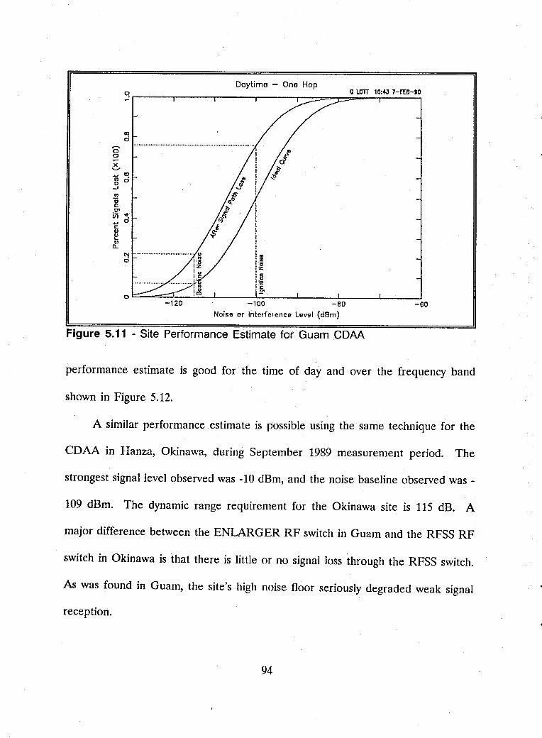
Daytime - One Hop G Lorr 10:43 7-fEB-90

qr-----.-----~------~----_r~~~~=---~----,

ID o 0' o .... )( '-'" .u ID

~ 0 -l

.!!! o c: 0' .- """ V1 •

.... 0 c: e III n.

o~~~~ __ ~~ ____ ~~ ____ _L ____ ~ ______ ~ ____ __l

-120 -80 -60 Noise or Interference Level (dBm)

Figure 5.11 - Site Performance Estimate for Guam CDM

performance estimate is good for the time of day and over the frequency band

shown in Figure 5.12.

A similar performance estimate is possible using the same technique for the

CDAA in Hanza, Okinawa, during September 1989 measurement period. The

strongest signal level observed was -10 dBm, and the noise baseline observed was -

109 dBm. The dynamic range requirement for the Okinawa site is 115 dB. A

major difference between the ENLARGER RF switch in Guam and the RFSS RF

switch in Okinawa is that there is little or no signal loss through the RFSS switch.

As was found in Guam, the site's high noise floor seriously degraded weak signal

reception.

94

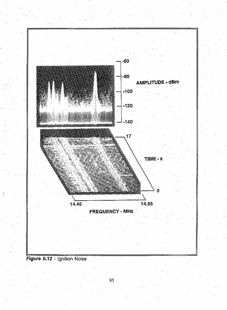
-60

AMPLITUDE - dBm

-100

TIME - s

-~o ,.

14.45 14.55

FREQUENCY - MHz .

Figure 5.12 - Ignition Noise

95

External noise from power-line related phenomena caused severe interference

at the Okinawa CDAA from 1.8 to 9 MHz. The worst power-line related noise

levels were near 3.5 MHz with an amplitude of -65 dBm. Using Figure 5.1, the site

cannot hear 100 percent of the daytime one hop signals of interest in the 2 to 6

MHz band while the power-line noise is present. The Hanza conditions result in

losing 90 percent of the nighttime one hop signals in the same band provided the

noise source was active at night. This power-line noise masks 100 percent of the

two hop signals in the frequency band from 2 to 6 MHz anytime the source is

active.

D. DISCUSSION

The site performance curves provide the field engineer and site personnel with

the first quantitative assessment of signals of interest lost due to RF system

deficiencies and noise. With performance estimates, one can prioritize problems

for correction. Fix-up programs can focus on the recovery of the maximum

quantity of signals lost. Site performance estimation has an important role in new

antenna site location decisions. All real estate considered for a new receiver site

requires a SNEP type survey before making a final site selection.

96

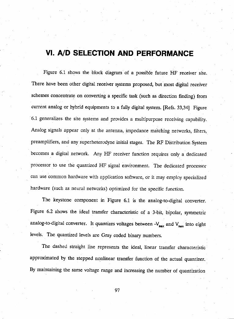
VI. AID SELECTION AND PERFORMANCE

Figure 6.1 shows the block diagram of a possible future HF receiver site.

There have been other digital receiver systems proposed, but most digital receiver

schemes concentrate on converting a specific task (such as direction finding) from

current analog or hybrid equipments to a fully digital system. [Refs. 33,34] Figure

6.1 generalizes the site systems and provides a multipurpose receiving capability.

Analog signals appear only at the antenna, impedance matching networks, filters,

preamplifiers, and any superheterodyne initial stages. The RF Distribution System

becomes a digital network. Any HF receiver function requires only a dedicated

processor to use the quantized HF signal environment. The dedicated processor

can use common hardware with application software, or it may employ specialized

hardware (such as neural networks) optimized for the specific function.

The keystone component in Figure 6.1 is the analog-to-digital converter.

Figure 6.2 shows the ideal transfer characteristic of a 3-bit, bipolar, symmetric

analog-to-digital converter. It quantizes voltages between -V max and V max into eight

levels. The quantized levels are Gray coded binary numbers.

The dashed straight line represents the ideal, linear transfer characteristic

approximated by the stepped n~nlinear transfer function of the actual quantizer.

By maintaining the same voltage range and increasing the number of quantization

97

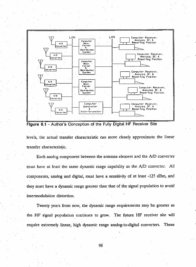
Conpl.Ater Be-on

forrler 8.

Distribution SysteM

COMputer BeOM

forMer 8.

Distribution Systel'l

COMput .. r Beol'l

rorne,.. 8.

Distribution SysteM

COMputer Gonloneter

8. InterferOME'tE'r

Figure 6.1 - Author's Conception of the Fully Digital HF Receiver Site

levels, the actual transfer characteristic can more closely approximate the linear

transfer characteris~.ic.

Each analog component between the antenna element and the NO converter

must have at least the same dynamic range capability as the NO converter. All

components, analog and digital, must have a sensitivity of at least -125 dBm, and

they must have a dynamic range greater than that of the signal population to avoid

intermodulation distortion.

Twenty years from now, the dynamic range requirements may be greater as

the HF signal population continues to grow. The future HF receiver site will

require extremely linear, high dynamic range analog-to-digital converters. These

98

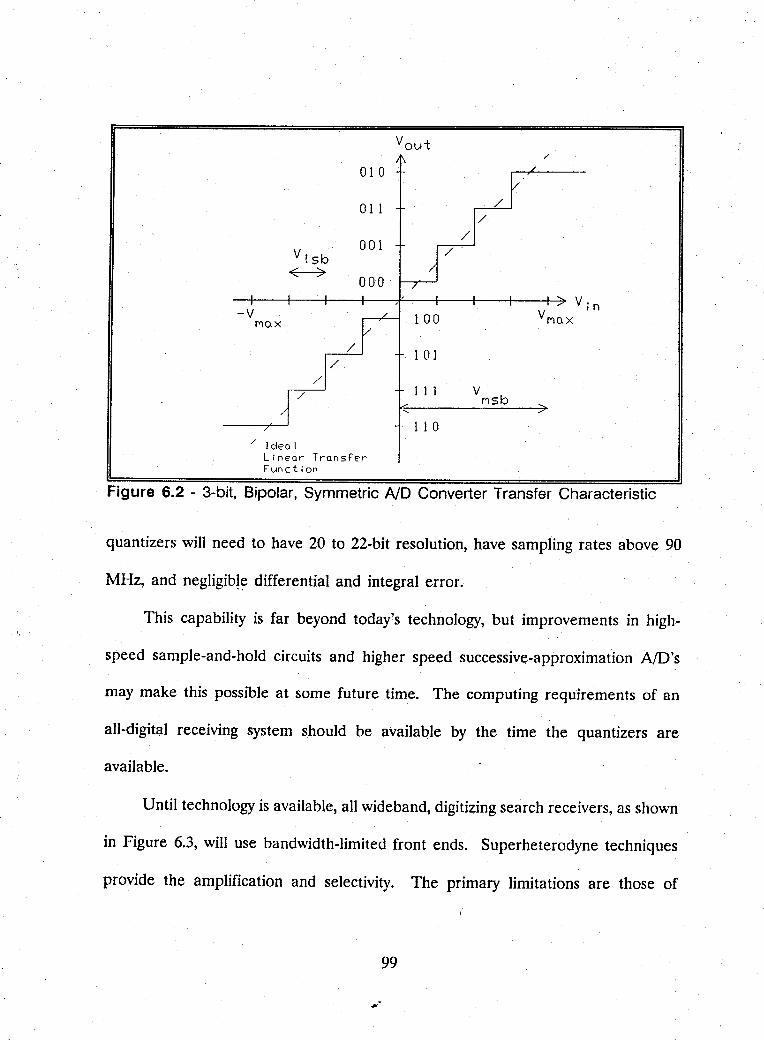
Voui: /

010

011

Vlsb 001

~ 000

-v --~--~--+---+---~--~---r--~---r~ Yin

VMOX MOX

/ I cleo t Llneor TronsFer Funct; on

100

1 01

111

1 1 0

V Msb

Figure 6.2 - 3-bit, Bipolar, Symmetric ND Converter Transfer Characteristic

quantizers will need to have 20 to 22-bit resolution, have sampling rates above 90

MHz, and negIigib!~ differential and integral error.

This capability is far beyond today's technology, but improvements in high-

speed sample-and-hold circuits and higher speed successive-approximation AID's

may make this possible at some future time. The computing requirements of an

all-digital receiving system should be available by the time the quantizers are

availabJe.

Until technology is available, all wideband, digitizing search receivers, as shown

in Figure 6.3, will use bandwidth-limited front ends. Superheterodyne techniques

provide the amplification and selectivity. The primary limitations are those of

99

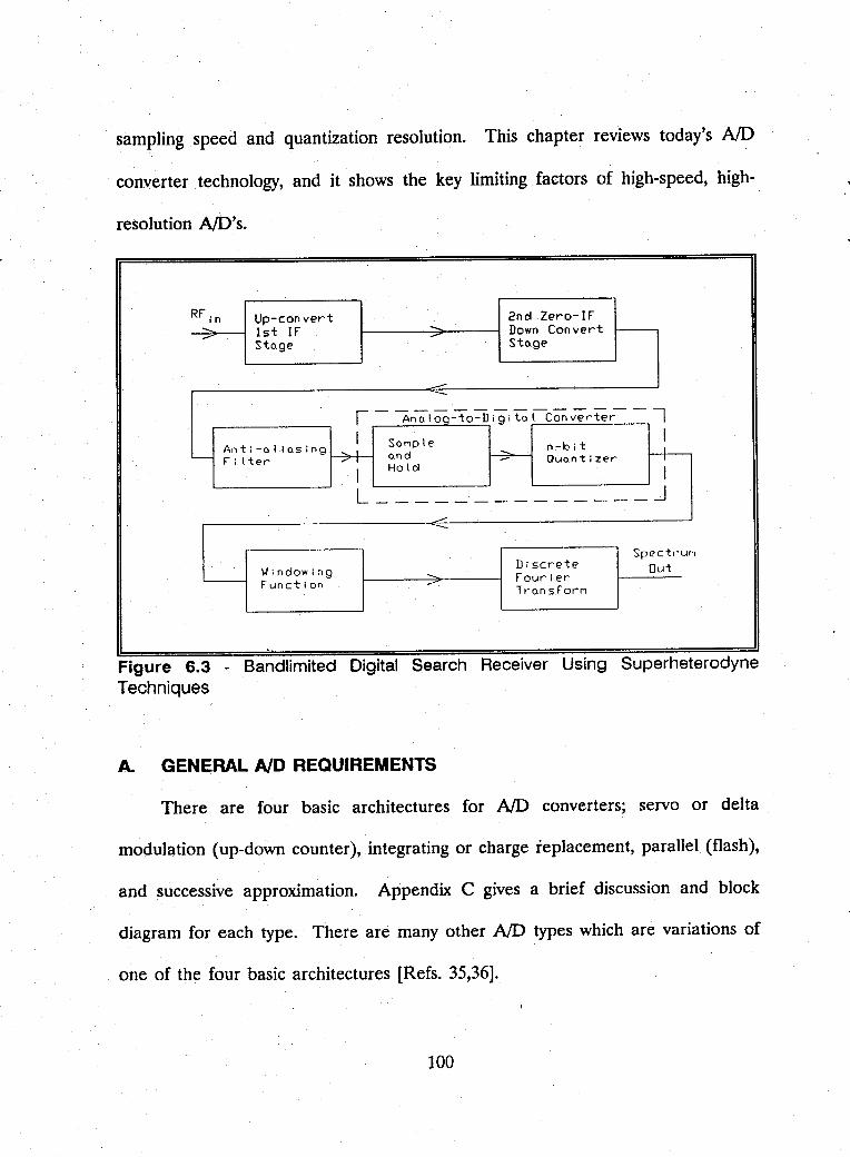
sampling speed and quantization resolution. This chapter reVIews today's AID

converter technology, and it shows the key limiting factors of high-speed, high-

resolution NO's.

RF;n Up-convert 2nd Zero-IF ..... 1st IF -. Down Convert - -Stage Stage

----1--------------, Anatoq-to-Digitot Converter

I SaMple n-bit I

Anti-at iasing f-+t-- ~ H-- r i I tel'" and Quantizer

I Hold I

L ______________ J

----Discrete

Spe Ct.-Uf"

Window i ng Out - ...... Fourier Function - lronsforM

Figure 6.3 - Bandlimited Digital Search Receiver Using Superheterodyne Techniques

A.. GENERAL AID REQUIREMENTS

There are four basic architectures for NO converters; servo or delta

modulation (up-down counter), integrating or charge replacement, parallel (flash),

and successive approximation. Appendix C gives a brief discussion and block

diagram for each type. There are many other NO types which are variations of

one of the four basic architectures [Refs. 35,36].

100

The requirements for an HF search receiver quantizerare:

• Large dynamic range

• Large value of sampling rate

• Excellent linearity.

Large dynamic range value equates to high resolution or to many bits in the

codeword which represents the input voltage. The highest resolution, off-the-shelf

converter is the 22-bit resolution Analog Devices Model AD1175K. It uses a multi

slope integrating technique. This converter ideally provides 133 dB dynamic range

with excellent linearity. [Ref. 37]

High-resolution quantization of HF signals requires receiver system

computational power with more bits to reduce the effects of round-off errors. High

speed 32-bit processors are just now becoming available to handle the processing

requirements.

Today's technology can provide only 10 to 16-bit resolution with conversion

speeds greater than 500 kHz. Rapid sampling is necessary to broaden the

bandwidth of each converter and to reduce the number of converters required to

cover the entire HF spectrum. The Nyquist sampling theorem requires a sampling

frequency twice the bandwidth coverage, but practice indicates that an all digital

receiving system requires a sampling frequency three to four times the bandwidth

coverage. The higher sampling frequency allows for better anti-aliasing filtering.

This is important since signals aliased into the passband reduce dynamic range.

101

Receiver coverage of the entire HF spectrum by dividing the 2 to 30 MHz

band into 8 to 15 bandwidth-limited segments is manageable both in equipment size

and overall control system requirements. This limited number of receivers requires

quantization of a bandlimited HF signal voltage by an NO converter sampling at

a frequency greater than 4 MHz. The single receiver performance limitation that

results from 22-bit quantizer resolution is a 10 kHz or less sampling frequency.

Receivers built using 22-bit NO converters may achieve the dynamic range needed

for today's HF signal population, but the resulting system requires as many

receivers as the narrowband search system mentioned in Chapter IV.

A high degree of NO converter linearity is necessary to prevent creation of

intermodulation (1M) products during quantization. 1M products are less of a

problem in narrowband digitizer schemes because most of the distorting signals will

appear outside the passband of the receiver .. In a wide bandwidth receiver, the 1M

products from many higher orders may fall in-band. This is particularly important

in an energy detection receiver where each in-band 1M product represents a new

. energy present condition.

With the HF spectrum's large number of signals, fading, extremely strong

signals, ionospheric effects, and strong man-made noise, the number of 1M products

by an NO converter without enough dynamic range could overwhelm a search

receiver system's ability to process all the new energies. The large signal

102

population may produce hundreds of IM products from only one strong station.

The result appears as broadband, white noise.

A dynamic-range-limited receiver system loses its weak signal detection

capability because in-band 1M products generate an increase in the system noise

floor. This broadband noise from 1M products increases the amplitude of the LTA

for each frequency bin. Weak signal amplitudes will no longer be greater than this

greater LTA value by the amount exceeding the amplitude screening threshold.

The resulting site performance degradation is the same as would be observed by

increasing the man-made noise level. The total noise voltage increase resulting

from ND nonlinearities must not exceed the voltage represented by the least

significant bit, or about 6 dB. In a 120 dB dynamic range system with a -125 dBm

noise floor, this equates to 1M products being less than one microvolt.

B. AID PERFORMANCE UMITATIONS

For the generalized HF new energy receiver, the following discussion assumes

that the system requires this level of performance:

• 120 dB dynamic range in a 1 kHz bandwidth

• 5 to 10 MHz sampling frequency

• Total nonlinearity related products no greater than one half of I-bit.

This section will discuss the bounds on receiver dynamic range performance

resulting from the quantization (ND conversion) process.

103

1. Aperture Uncertainty

The first device before the actual quantizer is a sample-and-hold (S/H).

The S/H is a type of voltage memory that retains the analog signal value while the

quantization process is underway. Much of the quantizing error results from

nonlinearities in the S/H [Ref. 38].

A simplified expression for the composite input signal voltage, with a

maximum frequency component fmax' as seen by the S/H is:

(6.1)

At the instant the sampling should take place, the incoming signal will be

changing at some rate. The slope of the incoming composite signal is:

The maximum slope occurs when:

where m is an integer.

t = (2m-1) 4fmax

(6.2)

(6.3)

In the S/H circuit, there are two operating modes, sample mode and

hold mode. During the sample mode, the output voltage ideally equals the input

voltage. The sample mode bandwidth of the S/H must be adequate to pass the

input signal without producing distortion. Otherwise the S/H is useless for that

104

application. During the hold mode, the output is held constant at the value of the

input signal at the instant when the SIH receives the hold command. [Ref. 39]

Aperture time is the duration of time from when the SIH receives the

command to switch from the sample mode to the hold mode to when the SIH

actually completes the transition and captures the input voltage level. The aperture

time will vary between devices, but it ideally should be a constant for a single

device. Actual SIH operation shows that the aperture time may vary within the

same device. This variability in aperture time is called aperture uncertainty. If the

input signal is changing rapidly, there can be a significant voltage change during the

aperture uncertainty period. The resulting error voltage is the difference between

the actual voltage level of the held signal from the voltage which was present when

the sample-to-hold transition should have been completed. [Ref. 39]

Aperture uncertainty is a random variable, but it has a maximum value

for a given physical device. This maximum time is the limiting value on the

resulting aperture uncertainty error.

Regardless of the statistics of the aperture uncertainty, the maximum

error should not exceed the voltage represented by one-half of the least-significant

bit (LSB) in the NO. The one-half LSB limit assumes that the input voltage is

uniformly distributed within one quantization interval.

The greatest error that can occur due to aperture uncertainty is that

occurring when the amplitude of the input signal is changing most rapidly. Let.,. a

105

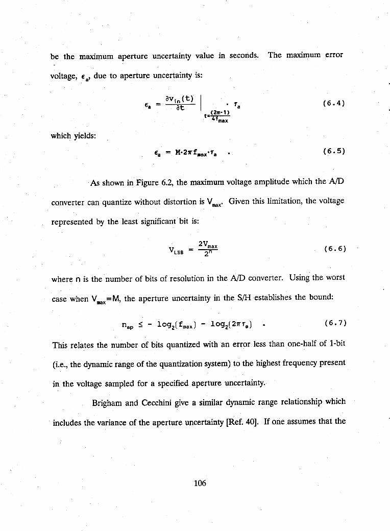
be the maximum aperture uncertainty value in seconds. The maximum error

voltage, € a' due to aperture uncertainty is:

(6.4)

which yields:

(6.5)

As shown in Figure 6.2, the maximum voltage amplitude which the NO

converter can quantize without distortion is V max' Given this limitation, the voltage

represented by the least significant bit is:

(6.6)

where n is the number of bits of resolution in the NO converter. Using the worst

case when V max = M, the aperture uncertainty in the S/H establishes the bound:

(6.7)

This relates the number of bits quantized with an error less than one-half of l-bit

(i.e., the dynamic range of the quantization system) to the highest frequency present

in the voltage sampled for a specified aperture uncertainty.

Brigham and Cecchini give a similar dynamic range relationship which

includes the variance of the aperture uncertainty [Ref. 40]. If one ,assumes that the

106

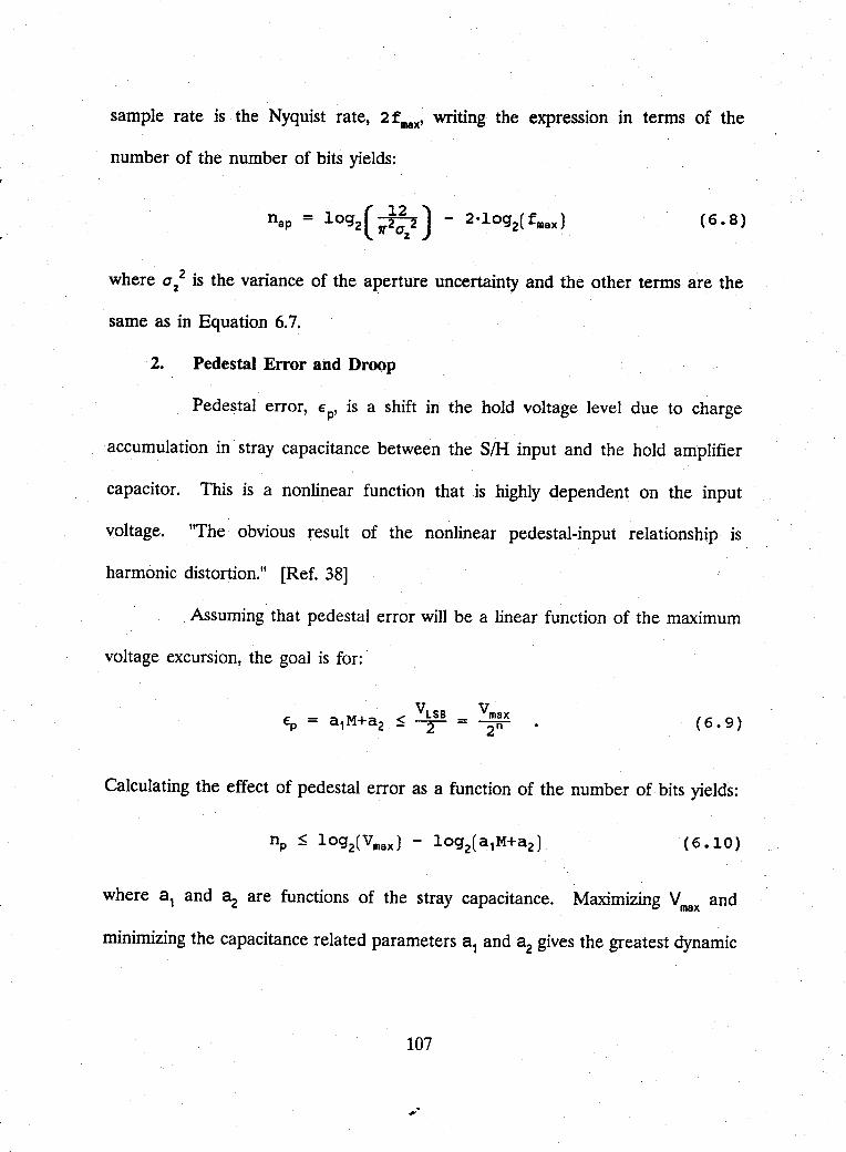
sample rate is the Nyquist rate, 2 fmax' writing the expression in terms of the

number of the number of bits yields:

(6.S)

where a z 2 is the variance of the aperture uncertainty and the other terms are the

same as in Equation 6.7.

2. Pedestal Error and Droop

Pedestal error, cp' is a shift in the hold voltage level due to charge

accumulation in stray capacitance between the S/H input and the hold amplifier

capacitor. This is a nonlinear function that is highly dependent on the input

voltage. "The· obvious result of the nonlinear pedestal-input relationship is

harmonic distortion." [Ref. 38]

Assuming that pedestal error will be a linear function of the maximum

voltage excursion, the goal is for:

(6.9)

Calculating the effect of pedestal error as a function of the number of bits yields:

where a, and a2 are functions of the stray capacitance. Maximizing V max and

minimizing the capacitance related parameters a, and a2 gives the greatest dynamic

107

-"

range. The bound established by pedestal error is not directly dependent on the

bandwidth .

. Droop error results from the gradual decay or change of the held analog

voltage. Many S/H devices use a charge storage device (i.e., a capacitor) to hold

the voltage level being quantized, and the stored voltage level will change with time.

The charge depletion results from finite resistances and parasitic capacitances to

ground associated with the hold circuit.

The entire NO conversion must occur before the droop error exceeds

one half of the ~B. Droop can cause significant error when used in conjunction

with slow conversion rate NO converters. Droop causes little error when used with

flash type converters since there is only one conversion cycle. Flash NO converters

are the type used in all high speed conversion systems like those in the broadband

HF receiver. Current design techniques can retain a stored voltage within one part

in 1 06 for a period less th~n 1 J.Ls. Therefore, the error resulting from droop in the

S/H is not a limitation on the HF receiver quantization process. [Ref. 38]

3. Analog Component Dynamic Range Limitations

Performance limitations in analog components which precede the S/H

and NO pair in a digitizing receiver can cause errors in the codeword generated

by the NO converter. A term used to describe this performance limitation of the

analog devices is spurious-free-dynamic-range (SFDR).

108

Understanding the performance bound resulting from analog component

nonlinearities requires the determination of two values. The first is minimum

detectable signal (MDS). MDS is the input power level to the quantizer due to

the kTB (thermal) noise voltage present; G, the analog front-end amplifier gain;

and, F, the analog front-end noise figure. The MDS is:

MDS = kTB·F·G (6.11)

where B is the bandwidth of the system feeding the S/H and NO pair. The MDS

value for the HFdigital search receiver should be less than -125 dBm.

The second value required is the third-order intercept point. This

number is used as an indicator of distortion resulting from the lumped effect of

nonlinearities in the active device. Determining the actual third-order intercept

point is usually done graphically. The third-order intercept point is the intersection

of the projection of the active device's linear gain characteristic and the linear

projection of the device's characteristic relating the power level of third-order 1M

products to the input signal power level. A device's manufacturer usually specifies

the third-order intercept point along with gain and noise figure.

By contrast, the values most often used to describe the lumped

nonlinearity errors in an NO converter alone are t~e differential error, the integral

error, and the effective number of bits [Refs. 41,42,43]. These three indicators of

NO performance are independent of the limitations of other devices.

109

In most systems, the third-order intermodulation products pro~uce the

greatest degradation in system dynamic range. This is true in a narrowband

superheterodyne receiver because the third-order 1M products are those that can

appear in-band and interfere with received signals. The third order intermodulation

product dynamic range is given as:

(6.12)

where DR3 is the third-order limited dynamic range and I30

is the third order

output intercept point [Ref. 44]. As shown before, the dynamic range of the

converter is 2" bits. Equating the two expressions yields:

2" = (6.13)

High dynamic range testing using a 1 Hz resolution bandwidth is an increasingly

common technique. The definition of SFDR for the analog devices is the ratio of

the third-order-output-intercept-point to the MDS in the 1 Hz bandwidth [Ref. 45].

The SFDR is not a directly measurable value since the third-order intercept point

is an extrapolated value. Using this definition, and changing the bandwidth B to

fmax' one can write the expression:

(6.14)

110

This expression equates the ideal dynamic range in bits to the

measurable dynamic range. This places another bound on dynamic range

performance as a function of the highest frequency sampled.

4. Quantization

Quantization error occurs because the quantization process maps a

continuous voltage into a subset of the integers. Figure 6.4 shows the error voltage

function resulting from the ideal NO transfer function. Between V max and -V max'

the error noise power of the ideal converter is due solely to quantization. The

quantization noise power, P q' in the uniform quantizer is:

Vmax

I ~(Vin) -Vmax

which when evaluated becomes:

2 VLSB

P = q 12

(6.15)

(6.16)

assuming that the voltage is uniformly distributed within each quantization step.

Gray and Zeoli developed an expression for NO quantization noise

based on the assumption that the input is Gaussian distributed with standard

deviation (] [Ref. 46]. By letting the value of (] times a positive integer k (k~ 1) be

111

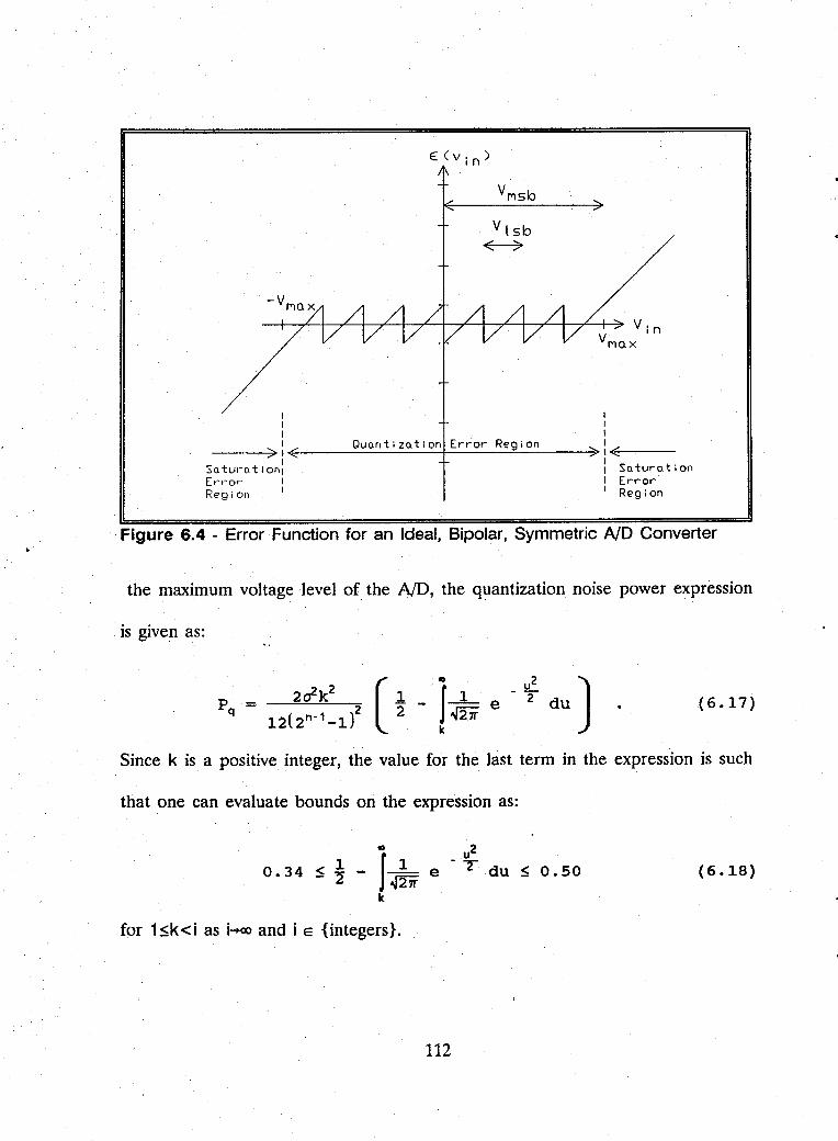
I I I I I I I Qunntizntion Error Region I

------~>I~----~~--~~~~~--~------~I~<------

Sntu.-otlon: : Soturntlon Error I I Error Region I I Region

Figure 6.4 - Error Function for an Ideal, Bipolar, Symmetric ND Converter

the maximum voltage level of the NO, the quantization noise power expression

is given as:

(6.17)

Since k is a positive integer, the value for the last term in the expression is such

that one can evaluate bounds ori the expression as:

1 0.34 :S "2 -

III

I~;7r k

for 1 :Sk<i as i-+oo and i E {integers}.

u2 -y

e du :S 0.50

112

(6.18)

For the ideal quantizer, where quantization noise and saturation are the

only limiting factors, the natural definition for dynamic range is the ratio of the

maximum power input to the NO without saturation, k2a 2, to the quantization

noise power, P q. Continuing with Gray and Zeoli's Gaussian input voltage

assumption, considering the case where n is large, and choosing the worst case from .

Equation 6.18, one can write the number of bits required to achieve a specified

dynamic range, DR, as:

1 "2 10g2 (DR) - 1. 07 = 0.167.DRdB - 1. 07 (6.19)

The effective number of bits is the same as in the ideal NO case, the

approximation of which was given in Equation 4.1. This function is a bound only

on the number of bits, and it is not a function of bandwidth.

In the HF signals case, the amplitude of the input signals are log-

normally distributed rather than being normally distributed as in the case above.

By assuming ideal, uniform. quantization, one can calculate the quantization noise

power for the HF signals as:

113

2 (In(xt r/ln)

2C7ln2 (6.20)

where {3 is the standard deviation of the distribution in Equation 3.9 and k{3 is the

voltage V max. In this case:

2

= (2~~ax) = (6.21)

resulting in the expression:

DR (6.22)

where

A (k{3) = (6.23)

One can then express the number of NO converter bits required as a function of

the specified dynamic range as:

(6.24)

or in dB as:

(6.25)

Since A(k{3):Sl, the last term in Equation 6.25 will reduce the effective

number of bits. For the case where A(k{3):::::l" the dynamic range changes at a rate

of 6 dB per bit which is the ideal case given in Equation 4.1.

114

5. Saturation

Saturation noise caused by overloading an NO converter is an important

consideration when working with signals in the HF band. Saturation severely

degrades system operation during nighttime at most HF receiver facilities. Today's

best amplifiers and multicouplers can barely process the daytime HF signal

population without producing intermodulation products. Since the HF signal levels

increase 20 to 30 dB at night, these stronger signals can easily exceed the input

voltage range for linear operation of the analog devices and the NO converter.

The devices become saturated, and the output noise level increases.

Saturation occurs when the amplitude of the input voltage being

quantized exceeds V max' Clipping is another term used to describe saturation.

While the quantization error voltage is a bounded, periodic value, the saturation

error voltage can grow without bounds. The limit on saturation is the total signal

capacity of the physical electronics before damage occurs.

By keeping the quantization step size small enough to reduce

quantization noise, the departure from a linear characteristic in the NO converter

transfer characteristic is kept small. While not truly a linear process, small

quantization step size minimizes the performance degradation resulting from

intermodulation products. Strong signal levels, which require a higher value of V max

for a given number of bits, result in greater quantization noise because the

115

quantization step size increases. Preventing saturation is a trade-off between

quantization and saturation noise for a fIxed quantizer resolution.

Figure 6.4 shows the region of input voltage values for which saturation

error occurs. The saturation error power is:

. (6.26)

By using symmetry, and writing the expression for the error voltage, the saturation

power becomes:

~ 2

Ps = 2· J ( v in - vmax { 1 - 2\ J) PVin(Vin) dVin

vmax

Further simplification of Equation 6.27 is possible when n is large.

(6.27)

Gray and Zeoli also developed an expression for NO saturation noise

using the same assumptions as in their quantization noise, case [Ref. 46]. Their

expression is:

(6.28)

116

Since saturation error is unbounded, simplification techniques used to

develop Equation 6.19 do not work with Equation 6.28. In the case of HF signals,

the saturation noise power for large values of n becomes:

II)

= 2· I (v in - kl3) 2

1 e kP vin ~27ra~n

(6.29)

As in the HF quantization noise case, there is no closed-form expression

deducible from Equation 6.29 to express the effective number of bits representing

true dynamic range as a function of saturation noise power. The best approach to

minimize the noise resulting from both quantization and saturation is to balance the

effects- through the optimal selection of the variable k. This can be done

numerically, and Gray and Zeoli did this for the Gaussian signal case [Ref. 46].

During the data collection described in Chapter IV, several data sets

were included to test the effects of NO saturation on the number of new energy

alarms. Figure 6.5 shows the equipment configuration used where paralleled 14-

bit and 12-bit NO converters quantized the same voltage. During the tests, strong

signal levels were present that would saturate either NO without adding some

front-end attenuation.

The experiment assumed that the number of new energies detected

during a 15 minute observation period would not change substantially from one

data set to another. This assumption requires the entire observation period to be

117

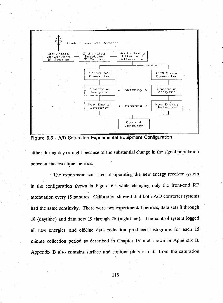
Conlcot-Monopote Antenno

1st Anolog Up-Conver:t IF Section

2nd Ano.tog Bo.sebo.nd

IF Section

____ no.tchlng _

____ no. tchlng ~

COMputer

Figure 6.5 - ND Saturation Experimental Equipment Configuration

either during day or night because of the substantial change in the signal population

between the two ti~e periods.

, The experiment consisted of operating the new energy receiver system

in the configuration shown in Figure 6.5 while changing only the front-end RF

attenuation every 15 minutes. Calibration showed that both NO converter systems

had the same sensitivity. There were two experimental periods, data sets 8 through

18 (daytime) and data sets 19 through 26 (nighttime): The control system logged

all new energies, and off-line data reduction produced histograms for each 15

minute collection period as described in Chapter IV and shown in Appendix B.

Appendix B also contains surface and contour plots of data from the saturation

118

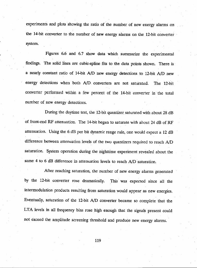
experiments and plots showing the ratio of the number of new energy alarms on

the 14-bit converter to the number of new energy alarms on the 12-bit converter

system.

Figures 6.6 and 6.7 show data which summarize the experimental

findings. The solid lines are cubic-spline fits to the data points shown. There is

a nearly constant ratio of 14-bit NO new energy detections to 12-bit NO new

energy detections when both NO converters are not saturated. The 12-bit

converter performed within a few percent of the 14-bit converter in the total

number of new energy detections.

During the daytime test, the 12-bit quantizer saturated with about 28 dB

of front-end RF attenuation. The 14-bit began to saturate with about 24 dB of RF

attenuation. Using the 6 dB per bit dynamic range rule, one would expect a 12 dB

difference between attenuation levels of the two quantizers required to reach NO

saturation. System operation during the nighttime experiment revealed about the

same 4 to 6 dB difference in attenuation levels to reach NO saturation.

After reaching saturation, the number of new energy alarms generated

by the 12-bit converter rose dramatically. This was expected since all the

intermodulation products resulting from saturation would appear as new energies.

Eventually, saturation of the 12-bit NO converter became so complete that the

LT A levels in all frequency bins rose high enough that the signals present could

not exceed the amplitude screening threshold and produce new energy alarms.

119

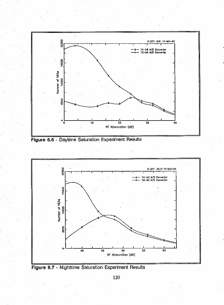
g o -,n ~

-6- 14-blt AID Converter -- 12-bit Io/D Connrter

°0~----~----~----~----~2~O----~----~30------~----~40

RF Attenuation (dB)

Figure 6.6 - Daytime Saturation Experiment Results

8 C LO"IT 10:17 17-t,t,\y-PO ~r--r---'----~---r----r---~---.----.r----r--~r---"

--tr- 14-bit AID Converhr -- 12-bit AID COllvsrier

OL-~ __ ~ ____ ~ __ ~ _____ ~ __ ~I ____ ~ __ -JI _____ L-__ ~ __ ~

40 ~ 50 55 60 RF Attenuation (dB)

Figure 6.7 - Nighttime Saturation Experiment Results

120

The 14-bit converter responded in a different way. During the daytime

test, the number of new energy alarms on the 14-bit system actually stabilized or

declined after saturation. Viewing the output spectrum from the receiver revealed

a different saturation phenomenon. The baseline noise level in the 12-bit converter

. gradually increased with each reduction of attenuation. This phenomenon

continued until there were no signals observable in the noise. However, the 14-

bit system had a marked jump in the baseline noise level upon reaching saturation.

This sudden addition of saturation noise caused the noise floor to increase by as

much as 20 to 30 dB. The result was a burst of new energy alarms activity upon

reaching saturation, but the LTA value for all frequency bins was already high

enough for no new alarms to occur.

The exact reason for the different saturation responses between the 12-

bit and 14-bit NO converters is not known, but one can hypothesize about the

causes. Both NO systems use different sample-and-hold amplifiers just prior to the

quantizer. If the compression rate of the S/H with the 14-bit converter's is greater

than that of the S/H with the 12-bit converter, the S/H with the 14-bit converter

would generate stronger 1M products of higher order than would the S/H amplifier

with the 12-bit converter. This would explain the sudden jump in the spectrum

with the 14-bit converter as explained above.

By measuring the slope of the lines in Figures 6.6 and 6.7 in the region

without NO saturation, one can write a simple expression for the change in the

121

number of new energy alarms as a function of added attenuation. When operating

without saturation, the rule-of-thumb is:

%~nea = o. 8'~RF Atten (dB) (6.30)

6. Aliasing

The performance of the lowpass filter which precedes the S/H and NO .

pair, as shown in Figure 6.3, places a limitation on the overall receiver system

dynamic range since the filter's out-of-band rejection is not infinite. Signals at

frequencies greater than one-half the sampling rate will be aliased into the receiver

passband unless attenuated by the anti-aliasing filter. A well designed filter can

substantially attenuate the voltage from the higher frequency signals, but the peak

out-of-band voltage levels must be no greater than one-half of the voltage

represented by the LSB, as shown in Figure 6.8. Otherwise, the aliased signals will

reduce system performance by interfering with weaker in-band signals.

In a digital search receiver, the final superheterodyne stage usually

translates the in-band signals to baseband (i.e., no frequencies greater than one half

the NO sampling rate). A receiver incorporating this superheterodyne method is

said to have a zero-IF final stage. In narrowband receiver design; " ... the anti-alias

filter requirements are generally more demanding in a digital radio than say for an

audio application where the signal energy above 15 kHz is small." [Ref. 47]

Traditional IF filter technology is adequate for narrowband receiver incorporating

122

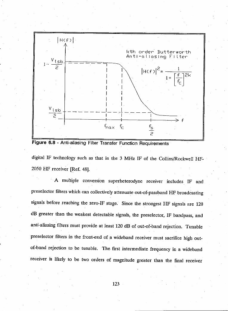
kth order Butterworth An t i -0. l i 0.5 i n 9 F i l ter

V l 5 b t-=~=-==-=~:-==-=::--_ 1- -2- --, 2 1

I /H(f)/ = ---: 1+ [:Jk I I I I I

Vlsb _______ I __ J. ____ _ I . I I

2 --+--------------+----~--------~------~_7.~ f

Figure 6.8 - Anti-aliasing Filter Transfer Function Requirements

digital IF technology such as that in the 3 MHz IF of the CollinslRockwell HF-

2050 HF receiver [~ef. 48].

A multiple conversion superheterodyne receiver includes IF and

preselector filters which can collectively attenuate out-of-passband HF broadcasting

signals before reaching the zero-IF stage. Since the strongest HF signals are 120

dB greater than the weakest detectable signals, the preselector, IF bandpass, and

anti-aliasing filters must provide at least 120 dB of mit-of-band rejection. Tunable

preselector filters in the front-end of a wideband receiver must sacrifice high out-

of-band rejection to be tunable. The first intermediate frequency in a wideband

receiver is likely to be two orders of magnitude greater than the final receiver

123

bandwidth, and realizable bandpass IF filters in such an up-conversion scheme lack

sufficiently steep skirts to provide the necessary out-of-band rejection. So the

greatest out-of-band filter rejection requirement in a wideband HF superheterodyne

receiver falls on the filter following the last frequency translation (the zero-IF

stage). This final filter is the anti-aliasing filter.

In addition to the out-of-band rejection requirement, Figure 6.8 also

shows that the anti-aliasing filter's passband ripple must be no greater than one-

half of V lsb. This places stringent requirements on Chebyshev, Bessel, and Elliptic

filter designs. To eliminate the ripple constraint from the analysis, the filter form

selected is the maximally-flat Butterworth form of a lowpass filter. The amplitude

transfer function for a Butterworth lowpass filter of order k is [Ref. 49]:

IH (f) I = 1

( f )2k

1+ -fc

(6.31)

Given a sampling frequency fs' the maximum out-of-band signal amplitude value

requirement is:

1

1+( 2~t) Vlsb < -- 2

124

(6.32)

In the filter passband, out to a frequency value of fmax' the transfer characteristic

must meet the condition that:

1

A special note is that fmax <fe'

Vlsb :S 1 - -2-

Rewriting Equation 6.32, with V max = 1, yields:

( f )2k

22n

- 1 = 2.:t

(6.33)

(6.34)

Substituting Equation 6.34 into Equation 6.33, and rearranging terms yields:

(6.35)

For a given sampling frequency and filter order, this expression provides the bound

on the dynamic range performance (in terms of the number of bits) as a function

of the bandwidth.

One can develop similar expressions for various filter forms using the

same criteria. Analysis of the elliptic, or Cauer, lowpass filter does not allow for

a closed form expression for the number of bits of dynamic range as given in

Equation 6.35. The Butterworth filter order, k, will be large to meet the 120 dB

dynamic range requirements. In practice, an exponential, Chebyshev, Bessel, or

Cauer form of anti-aliasing filter will be necessary.

125

For band-limited signal quantization, tt ••• a five-times sampling rate plus

a five-pole filter yields 0.5% aliasing error." [Ref. 50] This rule uses the natural

roll-off phenomenon to achieve the necessary out-of-band attenuation. In any case,

design should incorporate the highest sampling rate possible to further reduce

dynamic range limitations caused by the anti-aliasing filter.

7. Windowing and Round-ofT

Windowing places two limitations on the dynamic range performance of

the spectrum estimation form of the digital receiver. Sidelobes resulting from finite

sample lengths and main-lobe spreading resulting from the windowing function can

prevent detection of weak signals adjacent to strong signals. Rectangular windowing

does not produce small enough sidelobes for the required dynamic range.

There are two window functions which provide performance that

approaches the required sidelobe suppression. These are the Kaiser-Bessel (a=3.5)

and the Minimum 4-Sample Blackman-Harris windows. They provide 82 and 92

dB sidelobe suppression respectively. The tradeoff for dynamic range is that these

windowing functions produce main-lobe spreading. The equivalent noise bandwidth

is 1.93 and 2.00 bins respectively. [Ref. 51] Neither function provides the 120 dB

dynamic range necessary, so digital search receiver development must include

development of higher sidelobe suppressing window functions.

Finite register lengths for computing place dynamic range limitations on

the calculations required in the spectrum estimation portion of the digital search

126

receiver. These errors include the quantization of the windowing function itself,

the rounding or scaling of the FFf butterfly calculations, and the rounding of the

cosine and sine functions. There have been numerous studies of these effects .

. Computing power of today's processors allow 32 bit computations which provide

more than enough dynamic range. [Refs. 52,53]

C. COMBINED EFFECTS ON AID DYNAMIC RANGE

Several persons have developed methods for estimating the dynamic range of

an NO converter or a system which performs spectral estimation which has an NO

converter as a component part. Most of the estimating methods are in the form

of nomographs which allow rapid estimation of the dynamic range. Only Brigham

and Cecchini consider the entire system effect. [Refs. 40,54-57]

Figure 6.9 shows plots of the limiting effects on the number of bits (i.e.,

dynamic range) as given in Equations 6.8, 6.14, and 6.35 as a function of the

bandwidth (sampling rate) required. The lines drawn in Figure 6.9 are straight lines

connecting the data points calculated using the bounding equations. The shaded

region shows where today's technology is capable of operating. The desired

operating point marked is for a 2.5 MHz bandwidth (5 MHz sampling rate) and a

120 dB (20 bits) dynamic range. Steinbrecher performed a similar analysis of these

effects without considering the overall system performance requirements of the HF

digital receiver [Ref. 45]. Of the performance limiting effects mentioned in the

previous sections, only three, aperture uncertainty, analog component dynamic

127

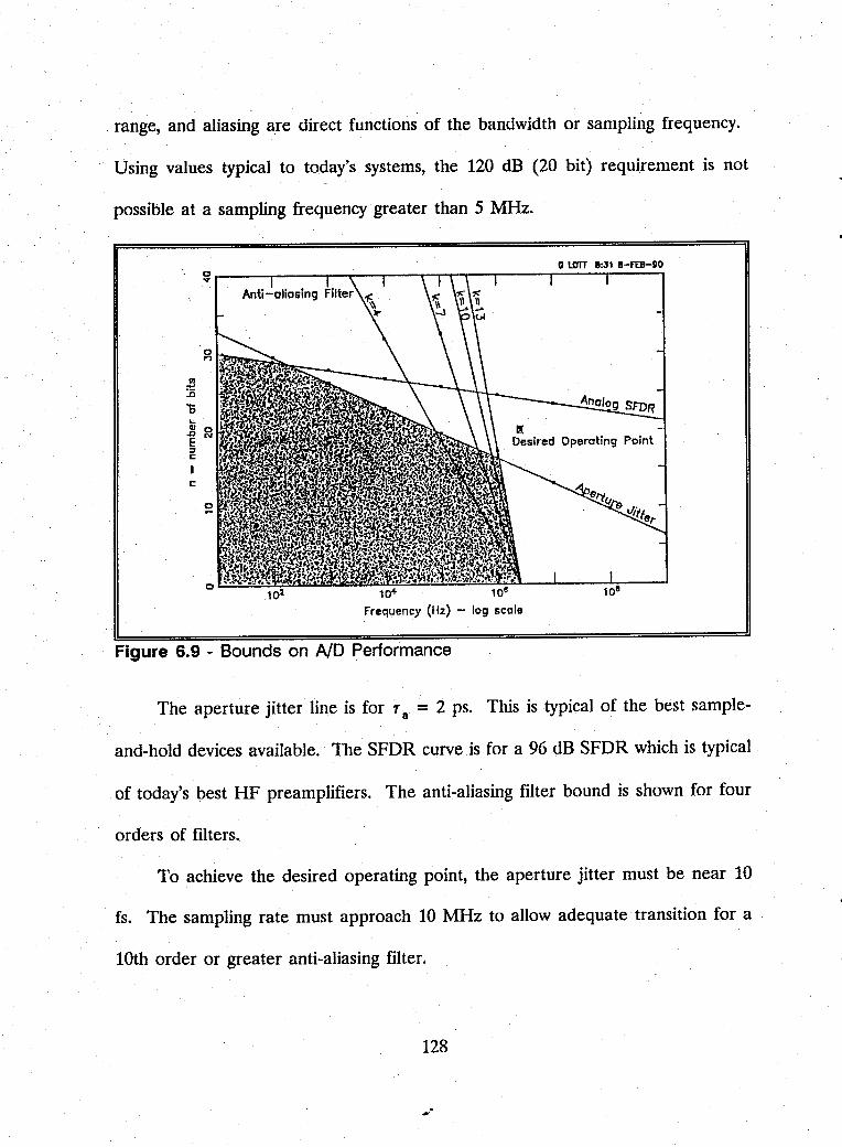
range, and aliasing are direct functions of the bandwidth or sampling frequency.

Using values typical to today's systems, the 120 dB (20 bit) requirement is not

possible at a sampling frequency greater than 5 MHz.

C LarT I!I:J 1 1!I-Ft:B-90 ~~--~----~-'---r---r~~--~----r---~~---'

~ ..c

(; ...

'0 n

Gl 0

E '" ::I c

104 108

Frequency (Hz) - log scale

Figure 6.9 - Bounds on ND Performance

The aperture jitter line is for r a = 2 ps. This is typical of the best sample-

and-hold devices available. The SFDR curve is for a 96 dB SFDR which is typical

of today's best HF preamplifiers. The anti-aliasing filter bound is shown for four

orders of filters.

To achieve the desired operating point, the aperture jitter must be near 10

fs. The sampling rate must approach 10 MHz to allow adequate transition for a

10th order or greater anti-aliasing filter.

128

Story performed a survey of NO conversion using an order-of-merit for each

type of converter. He concluded that the current performance limitations are at

70 dB with a 5 MHz sampling rate. Story's estimate closely matches the bounds

shown in Figure 6.9. His analysis shows about 2 dB of performance improvement

per year. [Ref. 58]

An analog-to-digital conversion system providing 120 dB dynamic range and

an adequate sampling rate is not likely to be available for some time. One must

explore ways to expand the dynamic range of today's technology.

129

VII. AID DYNAMIC RANGE EXTENSION METHODS

There is a continuing effort by both the Government and industry to produce

NO converters with high resolution and sampling rates greater than 1 MHz. A

rec~nt Government-sponsored research effort produced a 14-bit, 5-MSPS converter

[Ref. 59]. Commercial development produced a 12-bit, 10-MSPS converter which

received good trade reviews for RF signal processing applications [Refs. 60,61,62].

Hewlett-Packard has constructed a new NO converter and S/H combination which

provides lO-bits of resolution as 20-MSPS [Ref. 63]. There is even advance notice

of a 16-bit, 0.5-MSPS converter coming to the commercial market [Ref. 64].

U.S. Naval Ocean Systems Center researchers have achieved some success

with wider-bandwidth receiver systems which . incorporate high resolution NO

converters. One project considered the digitization of RF signals received by a

submarine towed-buoy antenna system. The quantized data from various sources,

including the antennas, is then time-division-multiplexed on a fiber-optic cable

connecting the towed buoy to the submarine. The project proposes with direct

conversion of VLF signals with frequencies up to 150 kHz and quantization of HF

signals within a 100 kHz bandwidth after being heterodyned to a lower intermediate

frequency. [Ref. 65]

130

The towed system uses a 12-bit, 5-MSPS Analog Devices NO and S/H

combination. Power consumption is an important consideration in the device

selection because of power limitations in the buoy, and the power consumption of

the Analog Devices pair is lower than others. Experimentation shows that aperture

jitter and spurious signal production from lumped nonlinearities in the NO limited

system performance.. Multiple-tone and notched-noise dynamic range testing

showed that the RF NO conversion system had a 67 dB dynamic range which is

within 5 dB (1-bit) of ideal device performance. [Ref. 65]

Today's hardware technology cannot produce the 20-bit, 5-MSPS converter

needed in the HF digital search receiver [Ref. 66]. How does one extend the

dynamic range of available conversion architectures? Is there a method which does

not require returning to a narrowband receiver structure?

A. GAIN-ADJUSTING AND FLOATING-POINT CONVERSION

The most common method used to expand NO dynamic range is that of gain

adjustment. In analog receiver technology, automatic-gain-control (AGe) is an

equivalent technique. The digitizing version usually takes either of two forms;

floating-point with scaling or parallel-scaled conversion.

Figure 7.1 shows the block diagram of a floating-point type NO converter.

The first quantization produces a number representing the exponent of the final

floating-point codeword. The second quantization produces the mantissa value.

The value from the exponent determines the programming of gain or attenuation

131

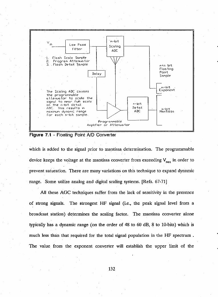
M-bit Low Po.ss

Fil ter 1---.---; Sco.ling 1---'----,

ADC

I. Flo. sh Sco.te So.Mple 2. Progro.M At tenuo. tor 3. Flosh Detoil SOMple

I Delo.y

TheScol~g ADC couses the progroMMo.ble ottenuo.tor to sco.le the Signo.l to neo.r full scole on the n-bit de to.il ADC. ThiS resul ts in MoxiMUM dynoMic ronge For eoch n-bit sOMple.

ProgrQMMo.ble AMplifier or Attenuo.tor

Figure 7.1 - Floating Point ND Converter

n-bit De to.il

ADC

M+n bit Flo 0. tlng POint SOMple

~M-bit . ~ponent -

n-bit - Mo.ntlssQ

which is added to the signal prior to mantissa determination. The programmable

device keeps the v~ltage at the mantissa converter from exceeding V max in order to

prevent saturation. There are many variations on this technique to expand dynamic

range. Some utilize analog and digital scaling systems. [Refs. 67-71]

All these AGe techniques suffer from the lack of sensitivity in the presence

of strong signals. The strongest HF signal (i.e., the peak signal level from a

broadcast station) determines the scaling factor. The mantissa converter alone

typically has a dynamic range (on the order of 48 to 60 dB, 8 to 10-bits) which is

much less than that required for the total signal population in the HF spectrum .

The value from the exponent converter will establish the upper limit of the

132

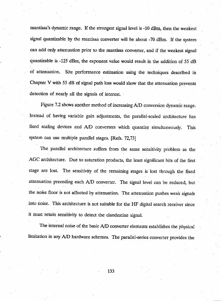
mantissa's dynamic range. If the strongest signal level is -10 dBm, then the weakest

signal quantizable by the mantissa converter will be about -70 dBm. If the system

can add only attenuation prior to the mantissa converter, and if the weakest signal

quantizable is -125 dBm, the exponent value would result in the addition of 55 dB

of attenuation. Site performance estimation using the techniques described in

Chapter V with 55 dB of signal path loss would show that the attenuation prevents

detection of nearly all the signals of interest.

Figure 7.2 shows another method of increasing ND conversion dynamic range.

Instead of having variable gain adjustments, the parallel-scaled architecture has

fixed scaling devices and NO converters which quantize simultaneously. This

system can use multiple parallel stages. [Refs. 72,73]

The parallel architecture suffers from the same sensitivity problem as the

AGC architecture. Due to saturation products, the least significant bits of the first

stage are lost. The sensitivity of the remaining stages is lost through the fixed

attenuation preceding each NO converter. The signal level can be reduced, but

the noise floor is not affected by attenuation. The attenuation pushes weak signals

into noise. This architecture is not suitable for the HF digital search receiver since

it must retain sensitivity to detect the clandestine signal.

The internal noise of the basic NO converter elements establishes the physical

limitation in any NO hardware schemes. The parallel-series converter provides the

133

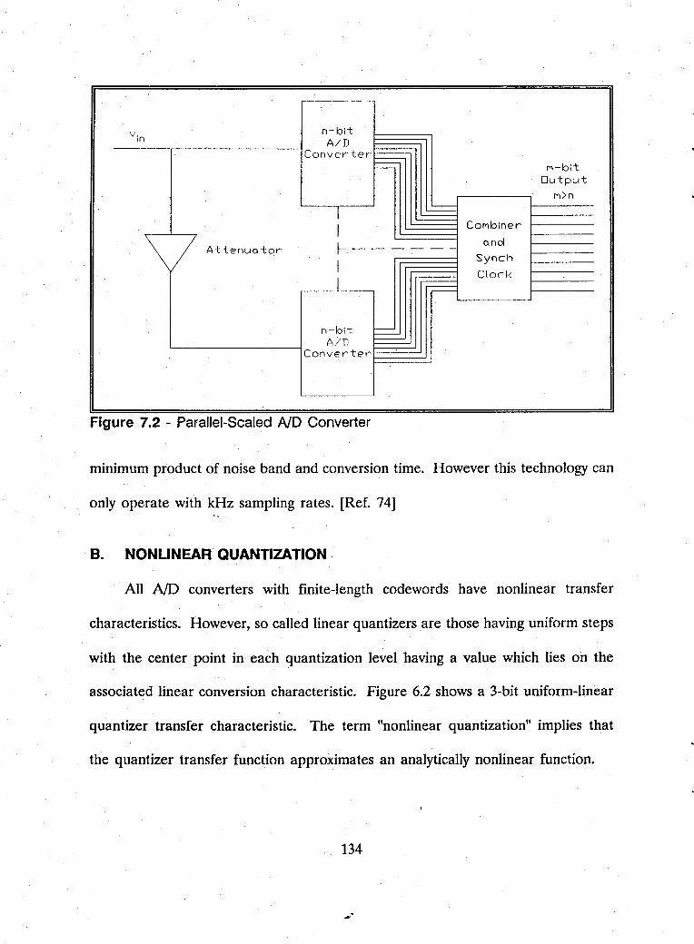
V in n-bit AID

Converter :::::=::-- M-bit

Output M>n

I --=== COMbiner I

\/ 1------- o.ncl Attenuo.tor

I Synch

I Clock

~

n-bit I AID I--

Converter

Figure 7.2 - Parallel-Scaled ND Converter

minimum product of noise band and conversion time. However this technology can

only operate with kHz sampling rates. [Ref. 74] "

B. NONLINEAR QUANTIZATION

AIl NO converters with finite-length codewords have nonlinear transfer

characteristics. However, so called linear quantizers are those having uniform steps

with the center point in each quantization level having a value which lies on the

associated linear conversion characteristic. Figure 6.2 shows a 3-bit uniform-linear

quantizer transfer characteristic. The term "nonlinear quantization" implies that

the quantizer transfer function approximates an analytically nonlinear function.

134

Nonlinear quantization has the analog equivalent of companding. Some

nonlinear quantization schemes incorporate a companding amplifier before a

uniform-linear NO. Another technique is to use linear quantization to precede a

digital nonlinear function converter stored as a look-up table in read-only-memory.

These two architectures are the easiest to implement. The more difficult technique

is direct nonlinear quantization where the nonlinear function is built directly into

the NO converter transfer characteristic through the implementation of variable

quantization step size. There are two basic techniques of direct nonlinear

quantization, fixed and adaptive.

Fixed, direct nonlinear converters have quantization step sizes which are set

in the hardware of the device. In an 8-bit square-root quantizer, the voltage step

which causes a change in the least significant bit at full scale is 55 dB more than

the voltage change causing a change in the least significant bit near zero [Ref. 75].

There have been many designs of nonlinear quantizers, and each has a

particular advantage for a specified application. "An analog-to-digital converter with

a square root transfer function will allow a maximum dynamic range with a fixed

number of data bits." The dynamic range covered by the quadratic converter is:

(7.1)

where n is the number of bits in the digital codeword. Transmitting video signals

from charged-coupled-device sensors over telemetry systems with limited data rates

135

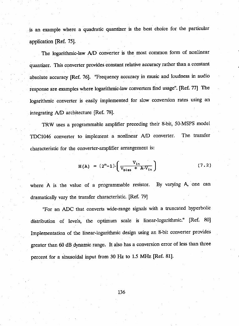
is an example where a quadratic quantizer is the best choice for the particular

application [Ref. 75].

The logarithmic-law NO converter is the most common form of nonlinear

quantizer. This converter provides constant relative accuracy rather than a constant

absolute accuracy [Ref. 76]. ''Frequency accuracy in music and loudness in audio

response are examples where logarithmic-law converters find usage". [Ref. 77] The

logarithmic converter is easily implemented for slow conversion rates using an

integrating NO architecture [Ref. 78].

TRW uses a programmable amplifier preceding their 8-bit, 50-MSPS model

TDC1046 converter to implement a nonlinear NO converter. The transfer

characteristic for the converter-amplifier arrangement is:

(7.2)

where A is the value of a programmable resistor. By varying A, one can

dramatically vary the transfer characteristic. [Ref. 79]

"For an ADC that converts wide-range signals with a truncated hyperbolic

distribution of levels, the optimum scale is linear-logarithmic." [Ref. 80]

Implementation of the linear-logarithmic design using an 8-bit converter provides

greater than 60 dB dynamic range. It also has a conversion error of less than three

percent for a sinusoidal input from 30 Hz to 1.5 MHz [Ref. 81].

136

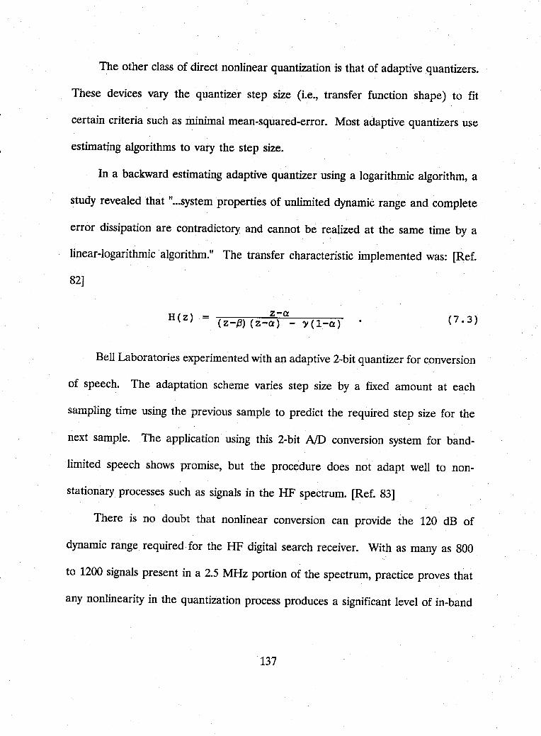
The other class of direct nonlinear quantization is that of adaptive quantizers.

These devices vary the quantizer step size (Le., transfer function shape) to fit

certain criteria such as minimal mean-squared-error. Most adaptive quantizers use

estimating algorithms to vary the step size.

In a backward estimating adaptive quantizer using a logarithmic algorithm, a

study revealed that 1I ••• system properties of unlimited dynamic range and complete

error dissipation are contradictory and cannot be realized at the same time by a

linear-logarithmic algorithm. II The transfer characteristic implemented was: [Ref.

82]

H(Z) = z-a (7.3) (z-~) (z-a) - Y(l-a)

Bell Laboratories experimented with an adaptive 2-bit quantizer for conversion

of speech. The adaptation scheme varies step size by a fixed amount at each

sampling time using the previous sample to predict the required step size for the

next sample. The application using this 2-bit AID conversion system for band-

limited speech shows promise, but the procedure does not adapt well to non-

stationary processes such as signals in the HF spectrum. [Ref. 83]

There is no doubt that nonlinear conversion can provide the 120 dB of

dynamic range required for the HF digital search receiver. With as many as 800

to 1200 signals present in a 2.5 MHz portion of the spectrum, practice proves that

any nonlinearity in the quantization process produces a significant level of in-band

137

intermodulation products that will mask weak signals. Any NO converter used in

an HF wideband receiver must have a transfer characteristic which is as close as

possible to a linear function. An NO converter with a uniform-symmetric transfer

function and small quantization step size (many bits) is the optimum choice for the

HF application.

c. OVERSAMPUNG

Oversampling is a technique in which one samples a signal at a rate which

is many times the Nyquist rate. By oversampling and decimation, one can extend

dynamic range of an NO converter by reducing quantization noise. Oversampling

spreads the quantization noise power evenly over a larger frequency interval, but

it does not alter the shape of the power spectrum of the noise. Decimation is an

averaging technique which acts as lowpass filtering of the higher frequency

quantization noise.

Practice shows that an effective dynamic range improvement of three to five

bits is possible with an oversampling factor in the range of 6 to 15. Figure 7.3

shows a plot of the gain in dynamic range in number of bits, nos' as a function of

the oversampling factor, fos' derived using Claasen's expression:

no. = - ~ 109,[ f:. ( 1 -

138

sin( -tJ 'ff

fos JJ (7.4)

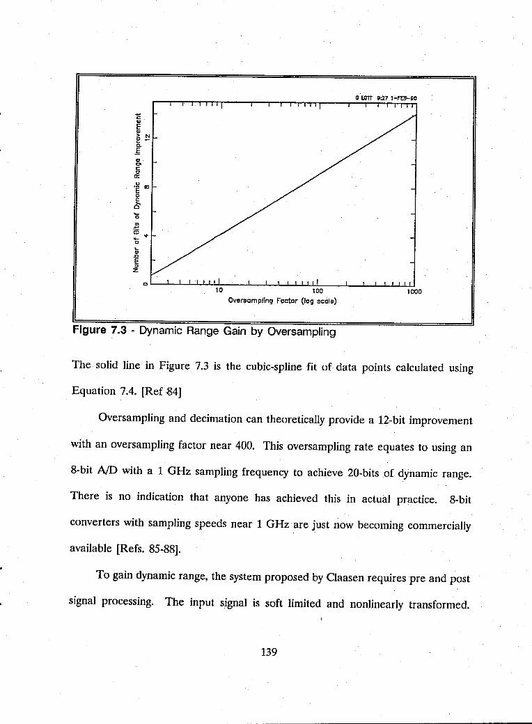
-c .. E .. > N 2 ~ Q.

f .. co c: o ct:

.~ CD E o

~ .... o

~ OJ ... .... c ... .. .s:J

E :2 Z

Overscmpllng Factor (log scale)

Figure 7.3 - Dynamic Range Gain by Oversampling

o lOTT 0:27 l-F'EB-OO

The solid line in Figure 7.3 is the cubic-spline fit of data points calculated using

Equation 7.4. [Ref -84]

Oversampling and decimation can theoretically provide a 12-bit improvement

with an oversampling factor near 400. This oversampling rate equates to using an

8-bit NO with a 1 GHz sampling frequency to achieve 20-bits of dynamic range.

There is no indication that anyone has achieved this in actual practice. 8-bit

converters with sampling speeds near 1 GHz are just now becoming commercially

available [Refs. 85-88].

To gain dynamic range, the system proposed by Claasen requires pre and post

signal processing. The input signal is soft limited and nonlinearly transformed.

139

After the NO conversion, the system takes first order differences followed by low

pass filtering in the form of decimation. [Ref. 84]

The oversampling reduces the quantization noise by a factor equal to fos. This

technique has worked in extending dynamic range in a 12-bit, 4-MSPS converter

[Ref. 89). In a narrow-band RADAR application, oversampling and decimation are

an effective dynamic range enhancing tool [Ref. 90). In each of these applications, .

the system processed a single signal and noise.

In a broadband HF receiver application, the pre-processing including soft

limiting and frequency modulation of the original signal will produce in-band

intermodulation products. These products are not noise in the sense of the

quantization noise, and they will appear in the output spectrum.

Oversampling also does not improve the sensitivity versus dynamic range. The

-125 dBm (0.2 IJ. V) sensitivity establishes the Il V requirement in the NO converter

(i.e., the voltage represented by the LSB). Even with quantization noise lowered

by oversampling, saturation of a limited dynamic range NO converter remains a

problem. There simply is no way to achieve a large signal handling capacity and

good sensitivity in an NO converter using Claasen's teChnique alone.

D. POST -CONVERSION PROCESSING

Extensive testing of NO converters reveals that the lumped effect of

nonlinearities within the device reduce the dynamic range. The lumped

nonlinearities include It ••• nonlinear distortion, quantization error, and random noise.1t

140

[Ref. 91] The value given as the effective number of bits better represents the

dynamic range of the system. For example, the Elsin AD1512, a 14-bit 5-MSPS

converter, loses 2-bits of dynamic range due to residual errors. [Refs. 92,93]

The El~in AD1512 was the NO converter in the receiver system used to

collect the data presented in Chapter IV. Ideally, a 14-bit NO converter should

have 84 dB of dynamic range using the six-dB-per-bit rule. Single-tone

measurements on the data collection system showed that the receiver had

approximately 73 dB (12-bits) of dynamic range. The performance measurement

closely matches the 12 effective bits for the Elsin converter measured by Lincoln

Labs [Ref. 92].

Linearization of the NO process recovers some of the information lost due

to unwanted distortion products. Compensation of the quantized signal

implemented through error table correction has proven as an effective means to

improve the number of effective bits. Conducting many discrete Fourier transforms

on the NO's output with a known signal input provides the statistical data needed

to determine the error table entries. [Ref. 94]

Error compensation on a Burr-Brown ADC600, 12-bit, 10-MSPS, improved

spurious-free-dynamic-range by 8 dB [Ref. 95]. Dent and Cowan proposed a

related correction technique for each NO before it leaves the factory [Ref. 96].

This method of dynamic range extension will bring converter performance closer

to the ideal.

141

Error compensation is a process with potential to improve the quantization

dynamic range in a digital search receiver. It will not, however, improve operation

to take today's NO technology to that required for the HF environment.

E. OTHER TECHNIQUES

The digital new energy receiver makes signal detection decisions based on

frequency domain representation of the input signal. Kay and Sudhaker presented

a method of spectrum estimation based on the measurements of the signal's zero

crossings. The computation speed requirements for the zero-crossing system are

within the speed capability of today's processors because the number of calculations

is similar to that required in the FFf algorithm. The system does not have the

limited amplitude dynamic range and slow conversion rates of a conventional NO.

There is no indication of the required precision of the zero-crossing measurement

needed for 120 dB dynamic range. There does not appear to be a published

implementation using this spectral estimation technique in any HF spectrum search

program, and it warrants further investigation since it is input signal amplitude

independent. [Ref. 97]

There have been many methods derived for quantization which minimize

mean squared quantization error by proper selection or adjustment of step size

[Refs. 98,99]. Bounds on optimal quantizer performance are well understood for

these 'cases [Refs. 100,101]. They do not always satisfy the sensitivity requirement,

especially when symmetric-uniform quantization is a requirement.

142

Sasaki and Hataoka propose a method of quantization which mInImIZeS

intermodulation distortion when the number of signals and number of quantization

levels is small. This technique does not work well with a large number of

quantization levels as required for adequate sensitivity in an HF receiver. It

provides no gain over the uniform-symmetric quantizerfor large numbers of bits.

[Ref. 102]

Other techniques under investigation include:

• digital Josephson circuits (SQUIDS) that do not latch into the voltage state [Ref. 103]

• photo conductor switched AID converters [Ref. 104]

• linear prediction with oversampling techniques [Ref. 104], and

• spectral estimation through hard clipping circuits[Ref. 105].

None of these techniques show direct application in the near-term to the HF search

receiver problem.

F. SUMMARY

. Dynamic error compensation is the dynamic range enhancing technique best

suited for implementation in an HF wideband receiver. Oversampling can improve

dynamic range, but the resulting intermodulation distortion will negate the

improvement. The HF receiver's performance requirements prohibit designs using

floating-point, AGe, and nonlinear quantization.

143

Converters with 14-bits and 20-MSPS are the next high dynamic range

improvements. 16-bit, 1-MSPS converters will also be available in the next few

years. Neither of these hardware improvements alone solves the HF new energy

receiver problem.

144

VIII. STRONG SIGNAL ELIMINATION

Chapters VI and VII show there are no NO techniques available today which

can achieve the performance required for the HF digital new energy re~eiver. The

strongest international broadcasting signal which sometimes reaches 0 dBm, the

amplitude of the weak clandestine signal-of-interest which is often near -125 dBm,

and the need for a sampling speed of at least 5 MHz in order to keep the

receiver's complexity manageable combine to place extreme demands on NO

performance.

The receiver sensitivity requirement is directly related to the signals of

interest, and the rapid sampling rate is necessary for a receiver system which is

economically realizable. Of the three extremes, only the high dynamic range

requirement caused by strong broadcast signals does not result from performance

needed to improve the detection of signals of interest. As proven by the results

given in Chapters III and IV, if the strongest signals were not present, the dynamic

range of the NO converter could be reduced substantially without loss of detection

performance.

How much of the international broadcasting energy must one remove to

reduce the dynamic range requirements? During Signal-to-Noise Enhancement -

Program site surveys, it is SNEP team practice to examine the overall HF signal

145

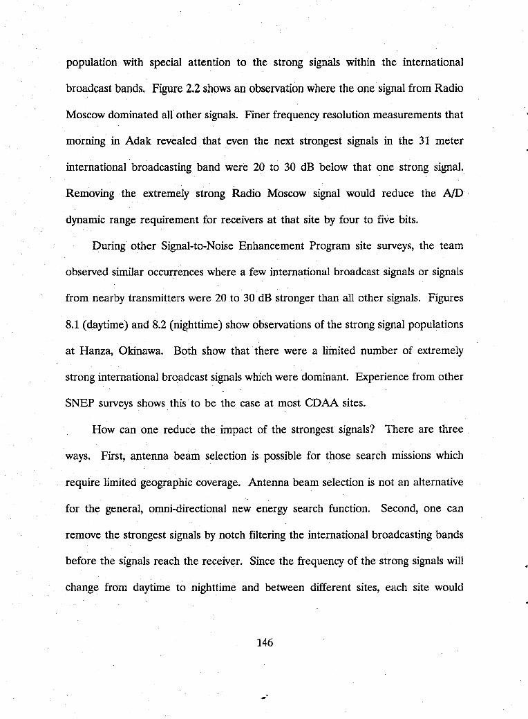
population with special attention to the strong signals within the international

broadcast bands. Figure 2.2 shows an observation where the one signal from Radio

Moscow dominated all other signals. Finer frequency resolution measurements that

morning in Adak revealed that even the next strongest signals in the 31 meter

international broadcasting band were 20 to 30 dB below that one strong signal.

Removing the extremely strong Radio Moscow signal would reduce the ND·

dynamic range requirement for receivers at that site by four to five bits.

During other Signal-to-Noise Enhancement Program site surveys, the team

observed similar occurrences where a few international broadcast signals or signals

from nearby transmitters were 20 to 30 dB stronger than all other signals. Figures

8.1 (daytime) and 8.2 (nighttime) show observations of the strong signal populations

at Hanza, Okinawa. Both show that there were a limited number of extremely

strong international broadcast signals which were dominant. Experience from other

SNEP surveys shows this to be the case at most CDAA sites.

How can one reduce the impact of the strongest signals? There are three

ways. First, antenna beam selection is possible for those search missions which

require limited geographic coverage. Antenna beam selection is not an alternative

for the general, omni-directional new energy search function. Second, one can

remove the strongest signals by notch filtering the international broadcasting bands

before the signals reach the receiver. Since the frequency of the strong signals will

change from daytime to nighttime and between different sites, each site would

146

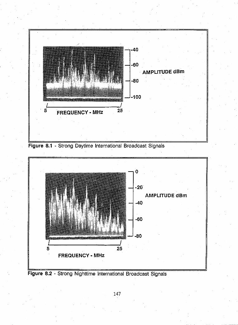
-40

-60 AMPLITUDE dBm

-80

-100

~/------------------~/ 5 FREQUENCY. MHz 25

Figure 8.1 - Strong Daytime International Broadcast Signals

o

·20'

AMPLITUDE dBm

·40

-60

·80

FREQUENCY - MHz

Figure 8.2 - Strong Nighttime International Broadcast Signals

147

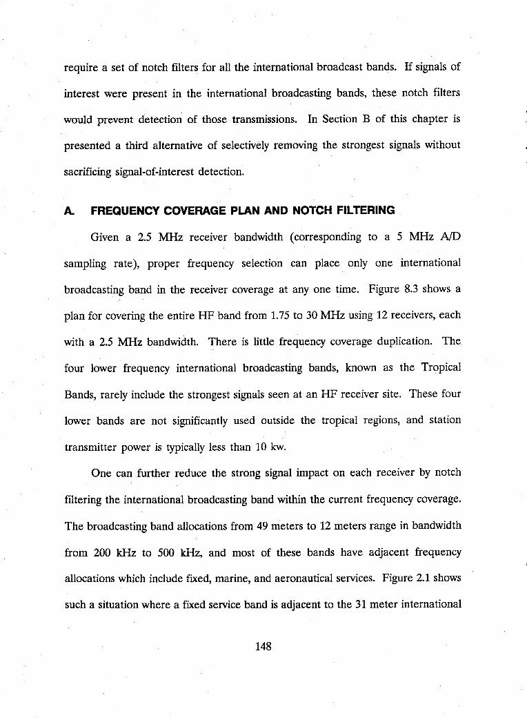
require a set of notch filters for all the international broadcast bands. If signals of

interest were present in the international broadcasting bands, these notch filters

would prevent detection of those transmissions. In Section B of this chapter is

presented a third alternative of selectively removing the strongest signals without

sacrificing signal-of-interest detection.

A. FREQUENCY COVERAGE PLAN AND NOTCH FILTERING

Given a 2.5 MHz receiver bandwidth (corresponding to a 5 MHz NO

sampling rate), proper frequency selection can place only one international

broadcasting band in the receiver coverage at anyone time. Figure 8.3 shows a

plan for covering the entire HF band from 1.75 to 30 MHz using 12 receivers, each

with a 2.5 MHz bandwidth. There is little frequency coverage duplication. The

four lower frequency international broadcasting bands, known as the Tropical

Bands, rarely include the strongest signals seen at an HF receiver site. These four

lower bands are not significantly used outside the tropical regions, and station

transmitter power is typically less than 10 kw.

One can further reduce the strong signal impact on each receiver by notch

filtering the international broadcasting band within the current frequency coverage.

The broadcasting band allocations from 49 meters to 12 meters range in bandwidth

from 200 kHz to 500 kHz, and most of these bands have adjacent frequency

allocations which include fixed, marine, and aeronautical services. Figure 2.1 shows

such a situation where a fixed service band is adjacent to the 31 meter international

148

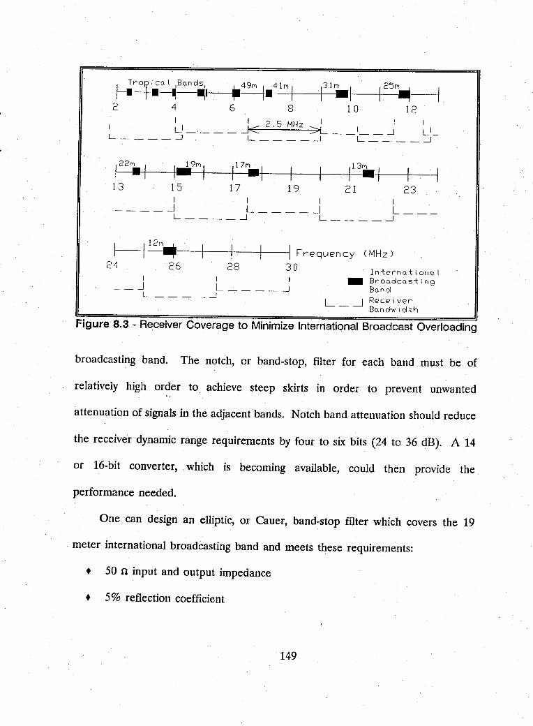
~~~~Bond~I ___ " 491'1 I_ 4_1--jM 1---j1f--31-11_--11----I--12-5�'1_----1 2 4 6 8 10 12

122.+I-~11-1~91'1~1 __ ~ll-7~I'1.HI--~~-~1-13~ •• 41--~~ 13 15 17 19 21 23

I I I I ____ ~ L ____ ~ L __ _ L ____ ~ L ____ ~

r---~--_+--~I Frequency (MHz) 24 28 30

I I I __ J L ____ ~

L ____ ~ -International Broadcasting Band

L I Rece i vel'" - ---1 Bandw i dth

Figure 8.3 - Receiver Coverage to Minimize International Broadcast Overloading

broadcasting band. The notch, or band-stop, filter for each band must be of

relatively high order to achieve steep skirts in order to prevent unwanted "

attenuation of signals in the adjacent bands. Notch band attenuation should reduce

the receiver dynamic range requirements by four to six bits (24 to 36 dB). A 14

or 16-bit converter, which is becoming available, could then provide the

performance needed.

One can design an elliptic, or Cauer, band-stop filter which covers the 19

meter international broadcasting band and meets these requirements:

• 50 n input and output impedance

• 5% reflection coefficient

149

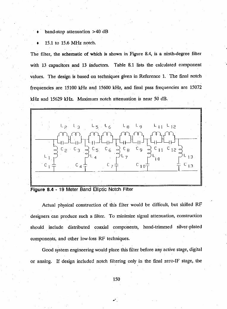
• band-stop attenuation >40 dB

• 15.1 to 15.6 MHz notch.

The filter, the schematic of which is shown in Figure 8.4, is a ninth-degree filter

with 13 capacitors and 13 inductors. Table 8.1 lists the calculated component

values. The design is based on techniques given in Reference 1. The final notch

frequencies. are 15100 kHz and 15600 kHz, and final pass frequencies are 15072

kHz and 15629 kHz. Maximum notch attenuation is near 50 dB.

L 5. L 6 L 11 L 12

Figure 8.4 - 19 Meter Band Elliptic Notch Filter

L 13

T C 13

Actual physical construction of this filter would be difficult, but skilled RF

designers can produce such a filter. To minimize signal attenuation, construction

should include distributed coaxial components, hand-trimmed silver-plated

components, and other low-loss RF techniques.

Good system engineering would place this filter before any active stage, digital

or analog. If design included notch filtering only in the final zero-IF stage, the ,

150

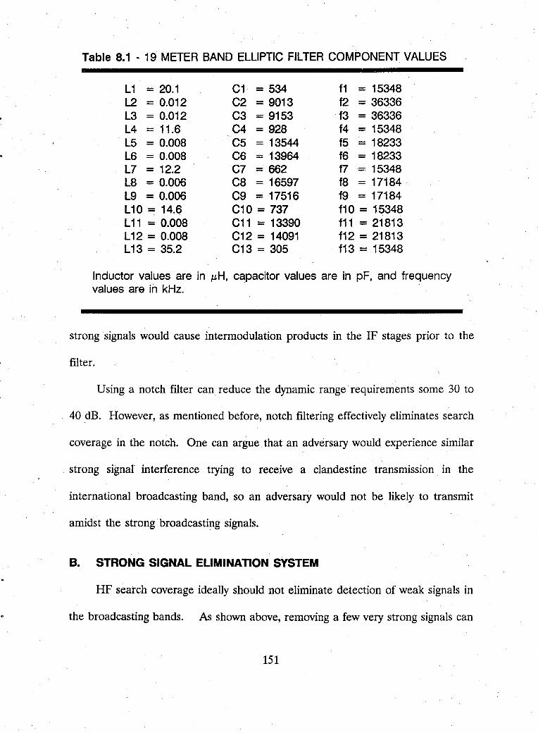
Table 8.1 - 19 METER BAND ELLIPTIC FILTER COMPONENT VALUES

L1 = 20.1 L2 = 0.012 L3 = 0.012 L4 = 11.6 L5 = 0.008 L6 = 0.008 L7 = 12.2 L8 = 0.006 L9 = 0.006 L10 = 14.6 L11 = 0.008 L12 = 0.008 L13 = 35.2

C1 = 534 C2 = 9013 C3 = 9153 C4 = 928 C5 = 13544 C6 = 13964 C7 = 662 C8 = 16597 C9 = 17516 C10 = 737 C11 = 13390 C12 = 14091 C13 = 305

f1 = 15348 12 = 36336 f3 = 36336 f4 = 15348 f5 = 18233 f6 = 18233 f7 = 15348 f8 = 17184 f9 = 17184 f10 = 15348 f11 = 21813 f12 = 21813 f13 = 15348

Inductor values are in J1.H, c~pacitor values are in pF, and frequency values are in kHz.

strong signals would cause intermodulation products in the IF stages prior to the

filter.

Using a notch filter can reduce the dynamic range requirements some 30 to

40 dB. However, as mentioned before, notch filtering effectively eliminates search

coverage in the notch. One can argue that an adversary would experience similar

strong signal interference trying to receive a clandestine transmission in the

international broadcasting band, so an adversary would not be likely to transmit

amidst the strong broadcasting signals.

B. STRONG SIGNAL ELIMINATION SYSTEM

HF search coverage ideally should not eliminate detection of weak signals in

the broadcasting bands. As shown above, removing a few very strong signals can

151

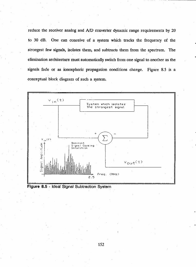
reduce the receiver analog and NO converter dynamic range requirements by 20

to 30 dB. One can conceive of a system which tracks the frequency of the

strongest few signals, isolates them, and subtracts them from the spectrum. The

elimination architecture must automatically switch from one signal to another as the

signals fade or as ionospheric propagation conditions change. Figure 8.5 is a

conceptual block diagram of such a system.

V. (f') ,n

OJ U :; +'

o c 0>

(/)

SysteM which iso\o.tes the strongest signo.\

DOMinont S;gnol Cous;ng Saturation

2.5

+

f'req. (MHz)

Figure 8.5 - Ideal Signal Subtraction System

152

In most cases, the strongest signal will be a double-sideband, with carrier, AM

signal from an international broadcasting station. Given this, one can represent the

composite HF voltage, vin{t), as:

(8.1)

where va{t), the strongest signal, is:

(8.2)

and vb{t), the sum of the remaining HF signals, is:

(8.3)

The ideal circuit design would allow for the isolation and complete elimination

of the strongest signal leaving the remaining components of the HF spectrum intact.

There will always be some error voltage since no system can reproduce va(t) exactly.

The elimination system must generate a carrier frequency signal in phase with the

carrier of the strongest signal. Isolation of the strongest signal also requires

detection of the signal's envelope with minimal corruption from the other signals.

1. Carrier Reconstruction

Some device in the strong signal elimination system must reproduce a

signal in-phase with the carrier of the strongest signal. Prof. Glen A. Myers has

developed such a phase tracking system [Ref. 106]. The complete system includes

153

--------------------------------------------------------------------------------~----

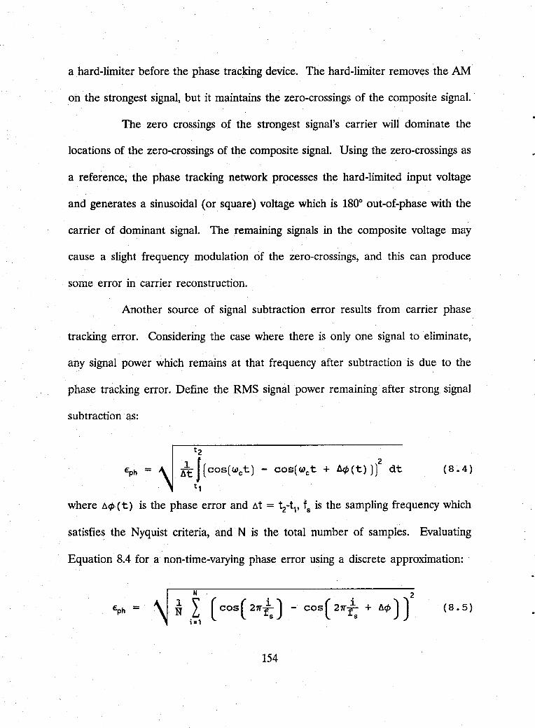
a hard-limiter before the phase tracking device. The hard-limiter removes the AM

on the strongest signal, but it maintains the zero-crossings of the composite signal.

The zero crossings of the strongest signal's carrier will dominate the

locations of the zero-crossings of the composite signal. Using the zero-crossings as

a reference, the phase tracking network processes the hard-limited input voltage

and generates a sinusoidal (or square) voltage which is 1800 out-of-phase with the

carrier of dominant signal. The remaining signals in the composite voltage may

cause a slight frequency modulation of the zero-crossings, and this can produce

some error in carrier reconstruction.

Another source of signal subtraction error results from carrier phase

tracking error. Considering the case where there is only one signal to eliminate,

any signal power which remains at that frequency after subtraction is due to the

phase tracking error. Define the RMS signal power remaining after strong signal

subtraction as:

tz

~\ J (cos(wet ) z

- cos( we t + ~¢ (t»)) dt (8.4)

t1

where t.¢·(t) is the phase error and t.t = tz-tl' fs is the sampling frequency which

satisfies the Nyquist criteria, and N is the total number of samples. Evaluating

Equation 8.4 for a non-time-varying phase error using a discrete approximation:

(8.5)

154

provides a simple rule for the amount of unwanted signal power which remains in

the single signal case. If one expresses the phase error in dB as:

(8.6)

the unwanted signal power which remains, in dBW, calculated using Equation 8.5

is:

(8.7)

Using the rule given in Equation 8.7 requires O<Llcp$O.1 radians. Using

Equation 8.5, a constant phase difference, Llcp, of 0.01 radians, is a phase difference

of -40 dB. The unwanted signal power which remains after subtraction is -43.1

dBW.

Since the goal of the strong signal elimination system is to decrease the

AID dynamic range requirements of the receiver by about 6 bits, the phase

reconstruction must be within 0.01 radians of the phase of the carrier of the

strongest signal. Testing proves that the device can lock well within the 0.01 radian

requirement when the signal is 10 dB or more greater than any other signal.

Can a filtered hard-limiter output alone adequately track the phase of

the strongest signal? If so, the circuit would be much simpler. Appendix D shows

a MATHCAD work sheet which simulates the complete large-signal-elimination

system using only a filtered hard-limiter output. Using a scaling value of 0.776 with

155

the hard limiter, the model showed that the filtered hard-limiter system could not

adequately remove the strongest signal. The weaker signal which was 20 dB down

remained undetectable because of the remaining unwanted signal energy. An

iterative process minimizing the error power identified the scaling factor of 0.776

as the value which produced the best subtraction of the strong signal.

2. Envelope Reconstruction

The second half of the strong signal reconstruction process is to isolate

the envelope of the strongest signal, A(t). This voltage is present in, but not easily

isolatable from, the composite signal envelope, E(t).

A preferred method requires an AM detector which exhibits capture

similar to that found in an FM detector. Then the output would allow construction

of A(t) alone. Yet there are no amplitude detectors developed which exhibit

capture.

Another method is to tune to the strongest signal using a conventional

AM receiver. Fading and multipath will result in the strongest signal changing

between several stations, so this electronically-tuned narrowband receiver would

need an extremely rapid tuning system.

156

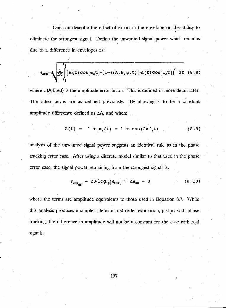
One can describe the effect of errors in the envelope on the ability to

eliminate the strongest signal. Define the unwanted signal power which remains

due to a difference in envelopes as:

t2

€amp= A\ I (A (t) cos( we t )-( l-€(A, B,cf>, t) )oA (t) cos( We t))2 dt (808)

t1

where €(A,B,cf>,t) is the amplitude error factor. This is defined in more detail later.

The other terms are as defined previously. By allowing € to be a constant

amplitude difference defined as flA, and when:

A(t) = 1 + rna (t) = 1 + cos (21Tfat) (8.9)

analysis of the unwanted signal power suggests an identical rule as in the phase

tracking error case. After using a discrete model similar to that used in the phase

error case, the signal power remaining from the strongest signal is:

(8.10 )

where the terms are amplitude equivalents to those used in Equation 8.7. While

this analysis produces a simple rule as a first order estimation, just as with phase

tracking, the difference in amplitude will not be a constant for the case with real

signals.

157

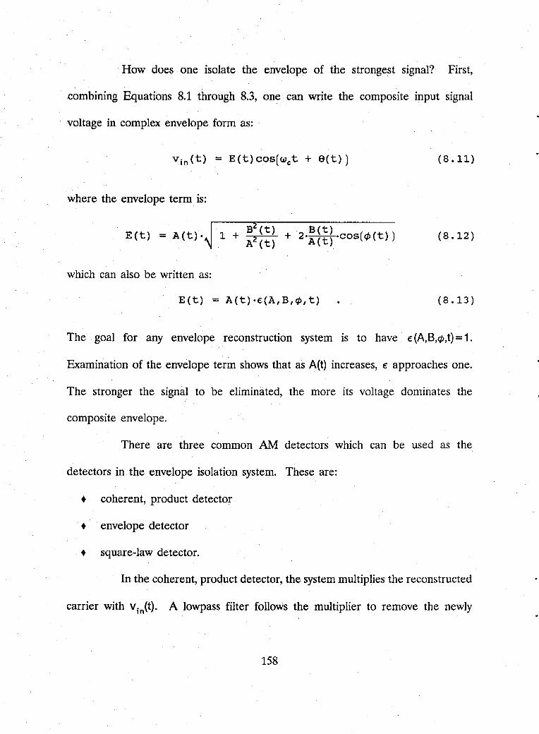
How does one isolate the envelope of the strongest signal? First,

combining Equations 8.1 through 8.3, one can write the composite input signal

voltage in complex envelope form as:

(8.11)

where the envelope term is:

E (t) = A (t)· B(t)

+ 2·A (t) .cos(cp(t) ) (8.12)

which can also be written as:

E(t) = A(t)·€(A,B,cp,t) (8.13)

The goal for any envelope reconstruction system is to have €(A,B,cp,t)=1.

Examination of the envelope term shows that as A(t) increases, € approaches one.

The stronger the signal to be eliminated, the more its voltage dominates the

composite envelope.

There are three common AM detectors which can be used as the

detectors in the envelope isolation system. These are:

+ coherent, product detector

+ envelope detector

• square-law detector.

In the coherent, product detector, the system multiplies the reconstructed

carrier with vin(t). A lowpass filter follows the multiplier to remove the newly

158

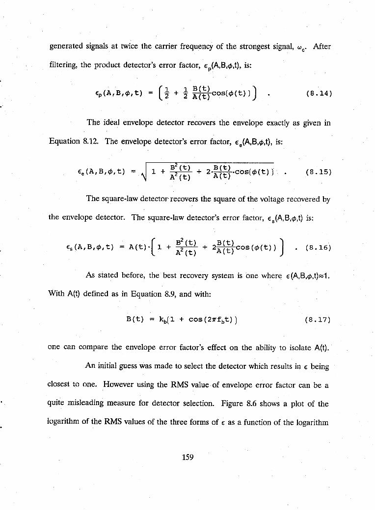
generated signals at twice the carrier frequency of the strongest signal, w c. After

filtering, the product detector's error factor, €p(A,B,¢,t), is:

(1 1 B(t) ) €p(A,B,¢,t) = 2" + 2" A(t) cos(¢(t») (8.14)

.'

The ideal envelope detector recovers the envelope exactly as given in

Equation 8.12. The envelope detector's error factor, €e(A,B,¢,t), is:

€e (A, B , ¢, t) = (8. 15)

The square-law detector- recovers the square of the voltage recovered by

the envelope detector. The square-law detector's error factor, €s(A.B,¢,t) is:

(8.16 )

As stated before, the best recovery system is one where € (A.B,¢,t)~1.

With A(t) defined as in Equation 8.9, and with:

(8.17)

one can compare the envelope error factor's effect on the ability to isolate A(t).

An initial guess was made to select the detector which results in € being

closest to one. However using the RMS value of envelope error factor can be a

quite misleading measure for detector selection. Figure 8.6 shows a plot of the

logarithm of the RMS values of the three forms of € as a function of the logarithm

159

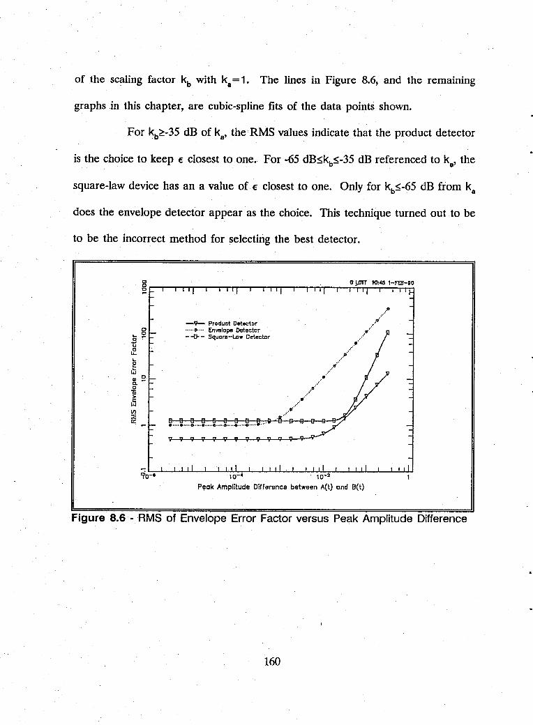
of the scaling factor kb with ka = 1. The lines in Figure 8.6, and the remaining

graphs in this chapter, are cubic-spline fits of the data points shown.

For kb~-35 dB of ka' the RMS values indicate that the product detector

is the choice to keep € closest to one. For -65 dB~kb~-35 dB referenced to ka' the

square-law device has an a value of € closest to one. Only for kb~-65 dB from ka

does the envelope detector appear as the choice. This technique turned out to be

to be the incorrect method for selecting the best detector.

. .•••••• 0

.••• 0

o ... 0 o ~

~ Product Detector ·····0···· Envslope Detector - -0- - Squc",-Law Detector

.... ,rt···

1:1 ~ .....

] QI ~ C. o Gi

~ VI ::z 0:: .····.····o>····o·····o·····o···· .. ····~···· "

.............. 0.

.•••• <1

.•.... If'

.• /<1

......•. ...... p .

90-- 10-4 10-2

Peak Amplitude Difference between A(t) and B(t)

Figure 8.6 - RMS of Envelope Error Factor versus Peak Amplitude Difference

160

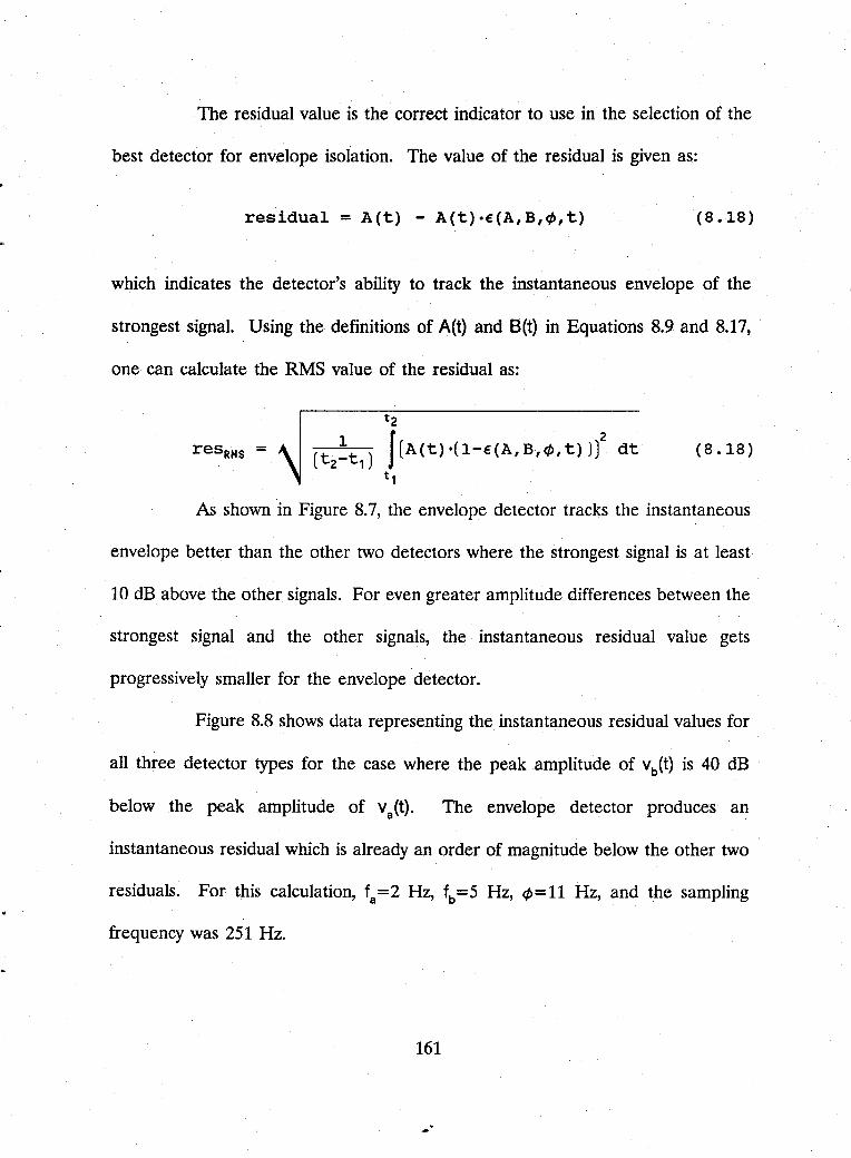
The residual value is the correct indicator to use in the selection of the

best detector for envelope isolation. The value of the residual is given as:

residual = A(t) - A(t)·~(A,B,¢,t) (8.18)

which indicates the detector's ability to track the instantaneous envelope of the

strongest signal. Using the definitions of A(t) and 8(t) in Equations 8.9 and 8.17, .

one can calculate the RMS value of the residual as:

resRMS = 1

t2

J(A(t).(1-~(A,B,¢,t»))2 dt

t, (8.18)

As shown in Figure 8.7, the envelope detector tracks the instantaneous

envelope better than the other two detectors where the strongest signal is at least

10 dB above the other signals. For even greater amplitude differences between the

strongest signal and the other signals, the instantaneous residual value gets

progressively smaller for the envelope detector.

Figure 8.8 shows data representing the instantaneous residual values for

all three detector types for the case where the peak amplitude of vb(t) is 40 dB

below the peak amplitude of Va (t). The envelope detector produces an

instantaneous residual which is already an order of magnitude below the other two

residuals. For this calculation, fa=2 Hz, fb=5 Hz, ¢=11 Hz, and the sampling

frequency was 251 Hz.

161

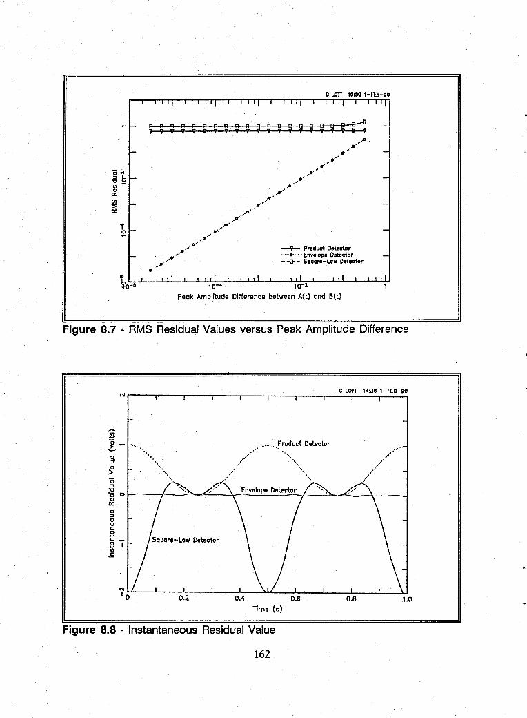
c u:m 10:50 1-ft8-;O I I I I I I I I I

-f- a 8 8 8 8 8 8 8 8 8 8 8 8 e 8 e 8 8 e e-S -V i V i i V i i i i V i i i i i i i V V V

.I>

r-.... 0···· -.'

C'-.••..•. 0 ............

0

.••••

~~ r- -VI •..... 0···· QI !l: .0····· V) .. ' :::;: r- .. ' -!l:

.0 .• ···"·····"

.. '

t -.••• 0 •• ••••••••

--.0'

~ Produd Detector f- •••••• 0 ••• ··0' .... •••••

·····0···· Envelop. ONdor -- -Go - Square-Law D..t.ctor

~-, t I I I I I I 10-4 10-2 1

Peck Amplitude Difference between A(t) and B(t)

Figure 8.7 - RMS Residual Values versus Peak Amplitude Difference

Nr-__ -.~---r ____ ._----r-__ -,-----r----,_ __ G~larr~~1~~'~38~1~-~rr=B~-~VO

,..... .l'.l

.~ - ~ ................ . ~ .......•

.........

CII ::I o III r: .B r:: ~I .E

. ........................ f.7.~.~ct Dutector

.................. . ................ .

TIme (s)

Figure 8.8 - Instantaneous Residual Value

162

0.8

.................. . ••.•...

. ....... .

1.0

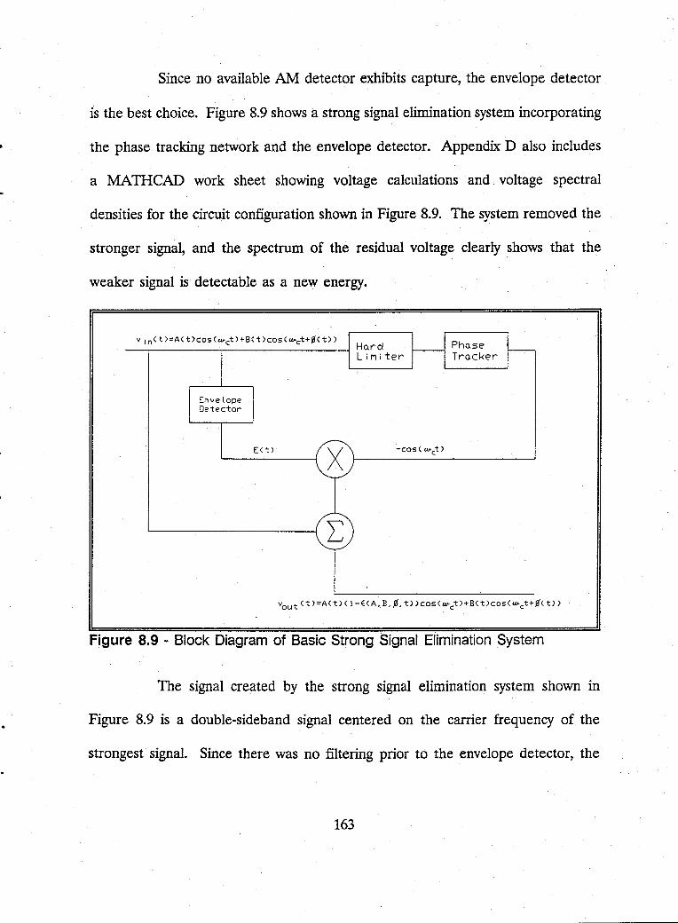
Since no available AM detector exhibits capture, the envelope detector

is the best choice. Figure 8.9 shows a strong signal elimination system incorporating

the phase tracking network and the envelope detector. Appendix D also includes

a MATH CAD work sheet showing voltage calculations and. voltage spectral

densities for the circuit configuration shown in Figure 8.9. The system removed the

stronger signal, and the spectrum of the residual voltage clearly shows that the

weaker signal is detectable as a new energy.

v In (t)=A( t)coS(Wct) +B( t )cos (W-ct+.a< t» Ho.rd Pho.se LiMiter

!---Tro.cker

i-----

Envelope Detector

E(t) X -cos (""ct)

L

Figure 8.9 - Block Diagram of Basic Strong Signal Elimination System

The signal created by the strong signal elimination system shown in

Figure 8.9 is a double-sideband signal centered on the carrier frequency of the

strongest signal. Since there was no filtering prior to the envelope detector, the

163

--------~-----

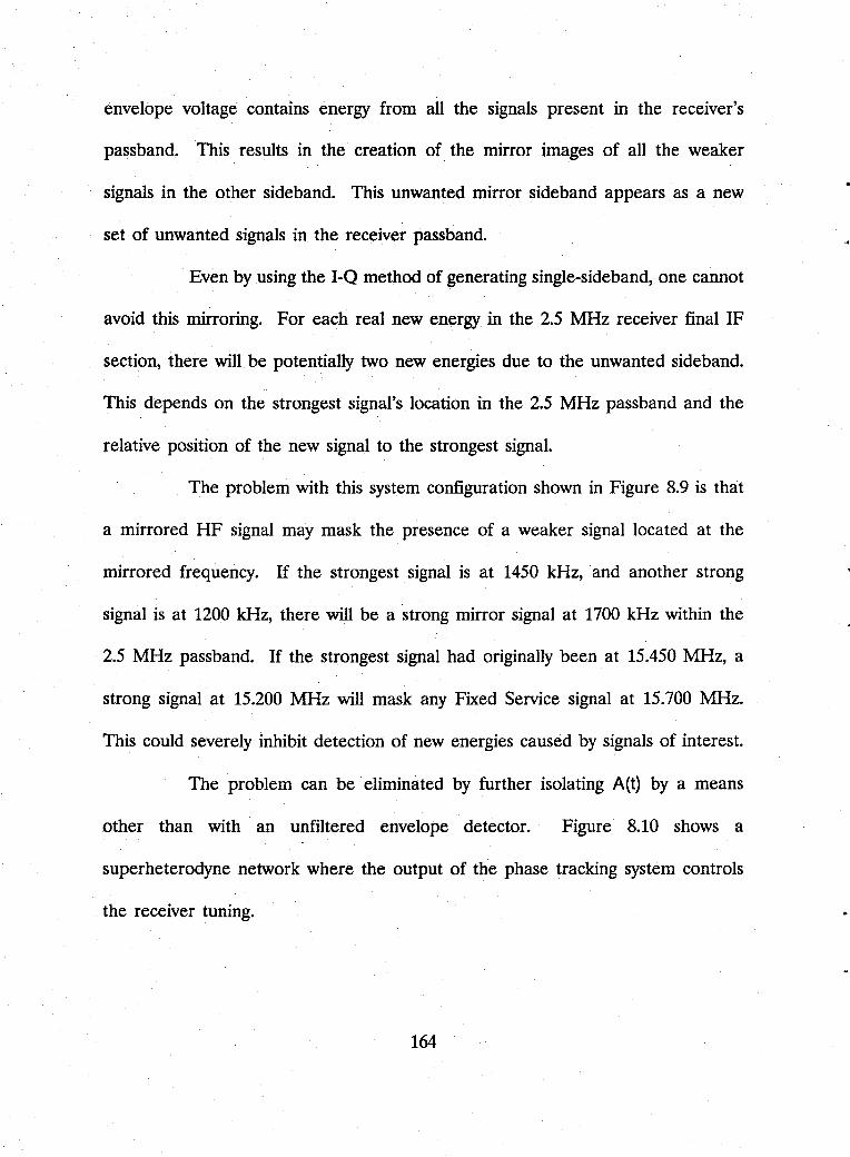
envelope voltage contains energy from all the signals present in the receiver's

passband. This results in the creation of the mirror images of all the weaker

signals in the other sideband. This unwanted mirror sideband appears as a new

set of unwanted signals in the receiver passband.

Even by using the I-Q method of generating single-sideband, one cannot

avoid this mirroring. For each real new energy in the 2.5 MHz receiver final IF

section, there will be potentially two new energies due to the unwanted sideband.

This depends on the strongest signal's location in the 2.5 MHz passband and the

relative position of the new signal to the strongest signal.

The problem with this system configuration shown in Figure 8.9 is that

a mirrored HF signal may mask the presence of a weaker signal located at the

mirrored frequency. If the strongest signal is at 1450 kHz, and another strong

signal is at 1200 kHz, there will be a strong mirror signal at 1700 kHz within the

2.5 MHz passband. If the strongest signal had originally been at 15.450 MHz, a

strong signal at 15.200 MHz will mask any Fixed Service signal at 15.700 MHz.

This could severely inhibit detection of new energies caused by signals of interest.

The problem can be eliminated by further isolating A(t) by a means

other than with an unfiltered envelope detector. Figure 8.10 shows a

superheterodyne network where the output of the phase tracking system controls

the receiver tuning.

164

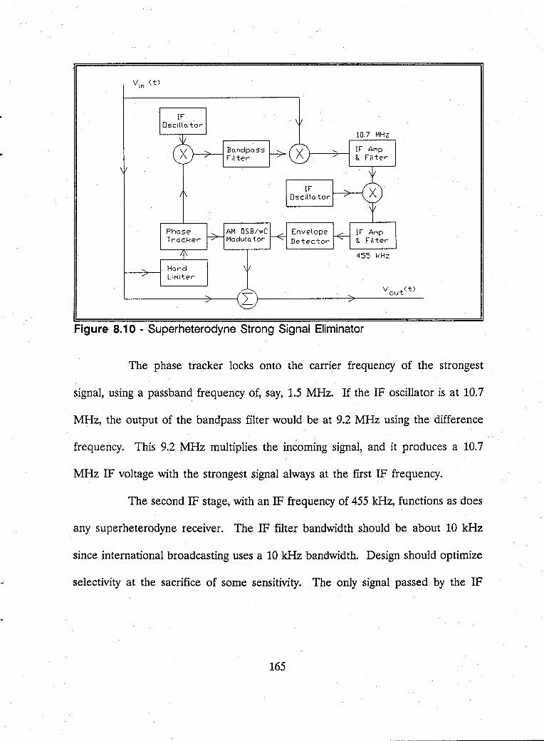
Figure 8.10 - Superheterodyne Strong Signal Eliminator

The phase tracker locks onto the carrier frequency of the strongest

signal, using a passband frequency of, say, 1.5 MHz. If the IF oscillator is at 10.7

MHz, the output of the bandpass filter would be at 9.2 MHz using the difference

frequency. This 9.2 MHz multiplies. the incoming signal, and it produces a 10.7

MHz IF voltage with the strongest signal always at the first IF frequency.

The second IF stage, with an IF frequency of 455 kHz, functions as does

any superheterodyne receiver. The IF filter bandwidth should be about 10 kHz

since international broadcasting uses a 10 kHz bandwidth. Design should optimize

selectivity at the sacrifice of some sensitivity. The only signal passed by the IF

165

stage will be the strongest signal. -There are many high-order filters available for

both the intermediate frequencies mentioned.

After the heterodyning and filtering, the envelope detector sees a voltage

which should contain only the IF form of va(t) and little, if any, other voltage

additionally from the other signals. The voltage from the envelope detector ideally

would be A(t).

The remaining design for subtraction is the same as shown in Figure 8.9.

The system reconstructs va(t) and subtracts it from the composite voltage vin(t).

There may be a phase error added due to delay in the IF circuits. If so, the

system may require an RF delay before the RF summer.

The system acts as the fast tuning receiver proposed earlier where the

tuning is slaved to the phase tracker. There is an order of magnitude increase in

the system's complexity, but there will be no mirroring of other signals. This system

can remove the strongest signal with little or no corruption of the other signals.

c. MULTIPLE-5TAGE STRONG SIGNAL EUMINATION

Figure 8.11 shows the application of multiple levels of strong signal elimination

in the RF system. The RF signals pass around the entire system until the peak

voltage level exceeds a threshold. The system switches in the strong signal

eliminators until the peak RF voltage drops below the saturation level. This system

can effectively expand the dynamic range of the digital receiver by altering the HF

signal environment before quantization takes place.

166

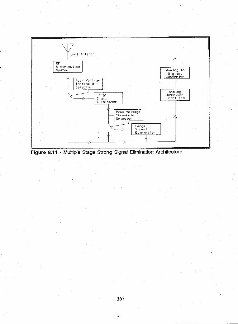
OMni Antenna.

Rr Distribution SysteM

Figure 8.11 - Multiple Stage Strong Signal Elimination Architecture

167

IX. CONCLUSIONS AND RECOMMENDATIONS

HF signal amplitudes are log-normally distributed. Their mean is 30 dB

higher at night than in the daytime. The nighttime variance is also higher. The

nighttime variance will range from about 40 to 140 depending on many variables.

Results from general HF spectrum surveys which target non-broadcasting

bands provide a good statistical description of the amplitude distribution of military

signals-of-interest. During daytime at a CDAA receiver facility, the mean level of

non-broadcast signals will be about -100 dBm. The nighttime mean will be near

-85 dBm. The probability distribution function for the military signals of interest

shows that the daytime signal amplitudes range over some 50 dB (-125 dBm to -

75 dBm), and the nighttime signal amplitudes range over 70 dB (-125 dBm to -55

dBm). Since the receiver front-end will receive energy from the international

broadcasting stations, the actual dynamic range required of an HF receiver is much

greater than that required only by the signals of interest. The receiver's dynamic

range must be at least 120 dB.

International broadcasting operations continue to grow, and broadcasting

signals are clearly the strongest signals in the spectrum. The strongest international

broadcasting signals will be 30 to 50 dB stronger than the strongest non

broadcasting signals. Intermodulation products in the RF Distribution System and

168

receivers resulting from these strongest signals corrupt the nighttime RF

environment at every Navy CDAA facility.

New energy receivers require a sensitivity of -125 dBm (0.2 J.l-V). The same

receiver must simultaneously process -5 dBm signals without intermodulation

distortion. Current receivers require large front-end attenuation to prevent

overload, and this attenuation causes a substantial performance loss.

The distribution of HF signal amplitudes provides a method of measuring HF

receiver site performance. Noise, interference, and signal path attenuation cause

poor performance. The peak value of noise and interference determines the

number of signals lost. Noise levels, temporally averaged, do not indicate the level

of degradation caused by man-made noise. RF Distribution System signal loss from

the antenna to the receiver should be kept to a minimum since it will reduce site

performance in a manner similar to increasing the external noise level.

In a digital, new-energy receiver, design should minimize the number of analog

devices (Le., amplifiers, switches) prior to the analog-to-digital converter. There

should be no electronic switching systems anywhere in the RF path as these

generate noise or attenuate the incoming signals. Where essential, analog systems

require special design to maximize their dynamic range in order to exceed the

dynamic range capability of the NO converter. Otherwise, 1M distortion will be

present when the input voltage is quantized. These 1M products can interfere with

actual signal detection.

169

Aperture uncertainty, saturation, aliasing, and intermodulation products bound

the performance capability in NO converters used in wideband HF receiver

applications. There currently exist NO converters with adequate dynamic range

for the HF spectrum, but these have slow sampling rates. Within the next ten

years, a 16-bit 5-MSPS converter will be available. A system built around a 16-bit

converter will have a 90 to 94 dB dynamic range.

Every quantizer in the new energy system should include dynamic error

compensation networks. Oversampling using the 1 GHz sampling converters will

reduce the quantization noise, but oversampling cannot provide the sensitivity and

dynamic range required in the HF new energy receiver.

Today, the only way to improve weak signal detection is to operate at the

NO converter performance threshold and to alter the HF signal environment.

Notch filtering can whiten the HF spectrum. Attenuating the international

broadcasting band signals by 40 dB reduces the dynamic range to about 80 dB.

However, weak signals of interest in the notched frequency bands are also

attenuated. So using notch filtering removes new-energy search coverage within the

stopband.

Altering the HF signal environment is the preferred way to improve

performance. Surveys show that a few signals constitute the front-end and NO

converter overloading. Frequency coverage should include only one international

broadcasting band within the receiver passband.

170

Large signal elimination is possible using a superheterodyne system. By

detecting the strongest signal's envelope, one can subtract the strongest signal

before quantization.

Many areas for research remain in this area. Future research should include:

• HF path-specific amplitude distribution studies. These should concentrate on polar, auroral, and trans-equatorial paths. There should be more work on the differences in one- and two-hop distributions.

• HF signal-specific amplitude distribution studies. The goal should be to create a subset of the non-broadcast signals including only military signalsof-interest.

• HF receiver site performance improvement verification. Studies should select one or two HF receiver sites which have measured poor performance. Work should identify and correct the problems. Operators should keep careful logs before and after the work. The experiment should define two or three operational performance indices. Using the performance curves in Chapter V, one should compare the operational indices to verify the improvement.

• Installation of broadcast band notch filters at a CDAA site. Studies should look carefully at before and after intermodulation products present in the receiver.

• Construction and testing of the large signal eliminator system.

171

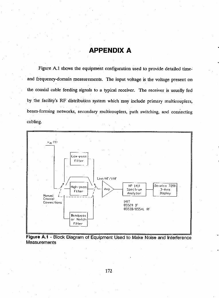
APPENDIX A

Figure A.l shows the equipment configuration used to provide detailed time-

and frequency-domain measurements. The input voltage is the voltage present on

the coaxial cable feeding signals to a typical receiver. The receiver is usually fed

by the facility's RF distribution system which may include primary multicouplers,

beam-forming networks, secondary multicouplers, path switching, and comlecting

cabling.

Low-pass r-- rilter t----

U.~ ~_~line8>-/HF/VHr HP 14!T Develco 7200 High-pass A

/ f--/ Mp SpectrUM - 3-AxiS I rilter I Ano.lyzer Displo.y

Mo.nuoJ L __________ -1

Coaxio.l 14!T Connections

Bo.ndpo.ss - or Notch t---

rilter

8552B Ir 8553B!8554L RF

Figure A.1 - Block Diagram of Equipment Used to Make Noise and Interference Measurements

172

While measurements are made with the spectrum analyzer connected directly

to the RF distribution system, filters and amplifiers can modify the input voltage.

The filters commonly used include a lowpass filter with a cutoff frequency of 1

MHz, a highpass filter with a 35 MHz cutoff frequency, and a bank of bandpass

filters designed to pass non-international broadcast bands from 2 to 30 MHz.

Strong signals may require the use of an external attenuator.

The amplifiers include a low frequency (10 Hz to 500 kHz) line amplifier, an

HF amplifier (such as the Olektron Model B-HIA-ll-HF, 500 kHz to 50 MHz),

and a VHF amplifier (50 MHz to 500 MHz). The line and VHF amplifiers are

used primarily to make intermodulation products measurements above and below

the HF spectrum. The HF amplifier must have a large dynamic range, requiring

a third order intercept point of at least + 52 dBm.

As shown in Figure A.l, the Hewlett-Packard (HP) Model 140/141 spectrum

analyzer acts as a scanning receiver. Along with the HP 141 T Display Section,

typical HF measurements require two plug-in modules, the HP 8552B Intermediate

Frequency Section and the HP 8553B RF Section. The operator can adjust the RF

attenuation, scan rate, scan width, IF gain, IF bandwidth, and other controls to give

the best presentation of the noise or signal under observation.

The Develco 7200 3-axis display provides a real time display of noise and

signals received with the spectrum analyzer. As shown in Figure A.2, the three

axes are usually frequency (horizontal axis), signal or noise power (vertical axis),

173

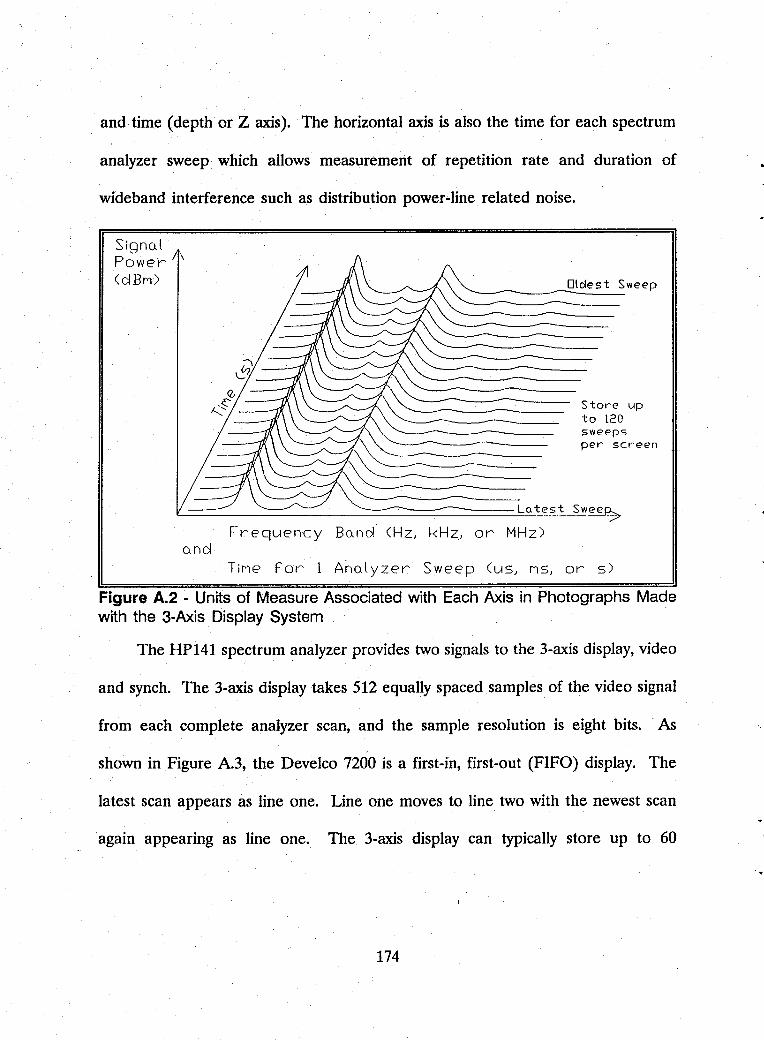
and time (depth or Z axis). The horizontal axis is also the time for each spectrum

analyzer sweep which allows measurement of repetition rate and duration of

wide band interference such as distribution power.;.line related noise.

Signed Power (clBf')

o.ncl

Oldest Sweep

Store up to 120 sweeps per screen

Latest Swee

Frequency Bo.ncl (Hz, KHz, or MHz)

Tif')e For 1 Ano.lyzer Sweep (us> f')S, or S)

Figure A.2 - Units of Measure Associated with Each Axis in Photographs Made with the 3-Axis Display System

The HP141 spectrum analyzer provides two signals to the 3-axis display, video

and synch. The 3-axis display takes 512 equally spaced samples of the video signal

from each complete analyzer scan, and the sample resolution is eight bits. . As

shown in Figure A.3, the Develco 7200 is a first-in, first-out (FIFO) display. The

latest scan appears as line one. Line one moves to line two with the newest scan

again appearing as line one. The 3-axis display can typically store up to 60

174

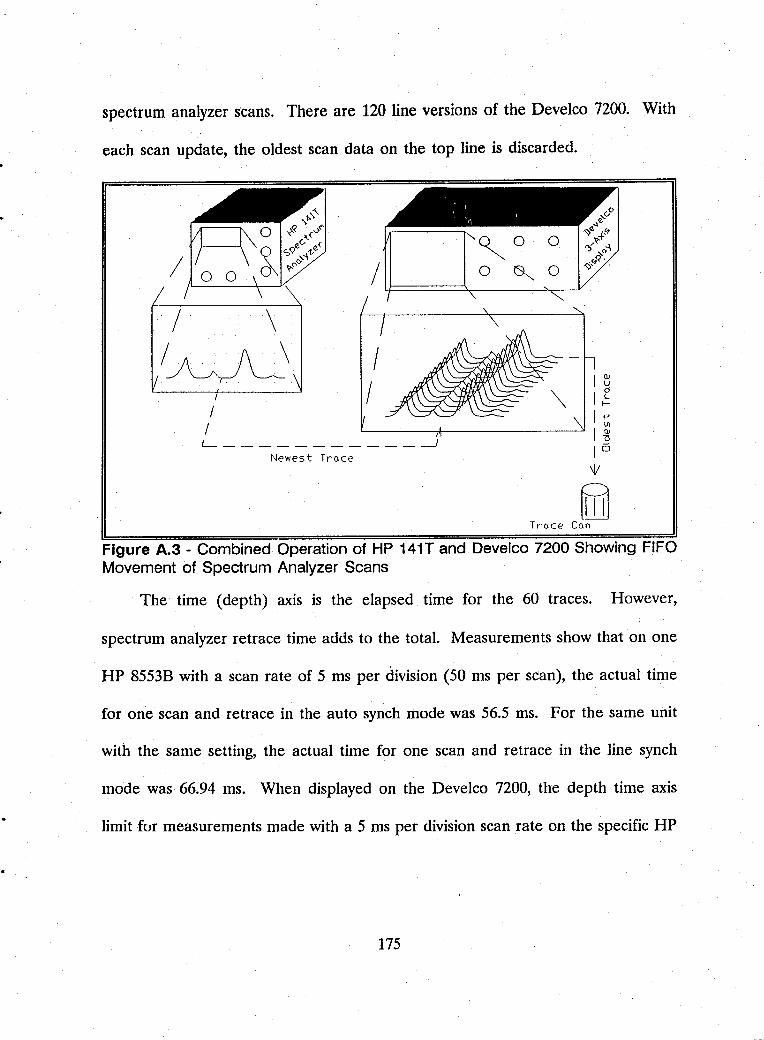
spectrum analyzer scans. There are 120 line versions of the Develco 7200. With

each scan update, the oldest scan data on the top line is discarded.

/ \ I~ I

I

Figure A.3 - Combined Operation of HP 141 T and Develco 7200 Showing FIFO Movement of Spectrum Analyzer Scans

The time (depth) axis is the elapsed time for the 60 traces. However,

spectrum analyzer retrace time adds to the total. Measurements show that on one

HP 8553B with a scan rate of 5 ms per division (50 ms per scan), the actual time

for one scan and retrace in the auto synch mode was 56.5 ms. For the same unit

with the same setting, the actual time for one scan and retrace in the line synch

mode was 66.94 ms. When displayed on the Deve1co 7200, the depth time axis

limit for measurements made with a 5 ms per division scan rate on the specific HP

175

8553B are 60 times the actual time for one scan plus retrace, or 3.4 sand 4.0 s

respectively.

There is no simple expression that one can use to determine the actual scan

time as a function of the instrument control scan rate. Prior to making

measurements, the operator must measure the actual scan times for each scan rate

in both the auto and line synch modes. The actual scan times will be different for

each HP 8553B, and experience shows that the times will change each time a unit

undergoes calibration.

Measurements require accurate frequency, amplitude, and time calibrations

for use as standards for manually scaling the photographs taken of the 3-axis

display'S screen. Calibrations include the total scan time measurements and a 10

dB step amplitude calibration photograph. Calibrations are good only for the

specific instruments used. Operators should make daily checks to ensure that the

calibration photographs are accurate. Changing the oscilloscope camera may

require a new amplitude calibration photograph because image compression may

occur due to small differences in the camera lens.

Figure A.4 shows a sketched example for 25 spectrum analyzer scans as

displayed on the Develco 7200. The figure shows the temporal changes for six

signals in the 50 kHz part of the HF spectrum. Actual signal identification for

some modulation types is difficult using only the 3-axis display. To make signal

identification easier, a separate HF communications receiver augments the

measurement system.

176

"'e 0. I-< FSK Signo.l

Two Stronger PSI-< Signo.ls

/~/---------------------------

12,55 Frequency (MHz) 12,60

On-Off Keying Morse Code

"'ide Bo.ndwidth Voice, FAX, Multitone

7 17,5

Tine (5)

Figure A.4 - Example of 3-Axis Display of HF Signals

The 3-axis display controls allow for:

• freezing the data in memory for photographing or detailed viewing

"

• changing amplitude compression

• changing the elevation and azimuth of the depth axis

• adjusting the background level.

To make photographs for amplitude measurements, the display elevation and

azimuth are set to zero. This results in viewing all 60 traces as if they were

superimposed into one trace. Using a card made from the 10 dB calibration step

photograph, knowing the equipment settings, and using the trace baseline as a

reference, one can manually scale the amplitude photographs.

177

Controls also allow for the selection and display of subsets of the 60 spectrum

analyzer scans stored in 3-axis display memory. Experience using the 3-axis display

while viewing various types of signals and noises results in the operator being able

to adjust the 3-axis display controls to optimize the presentation. A typical

measurement requires two photographs, one for amplitude measurement and one

with. the time (depth) axis elevated to show temporal variations.

178

APPENDIX B

This appendix contains histograms from data sets collected at the CDAA HF

receiver facility in Edzell, Scotland, during the period 10 - 22 April 1989. The main

discussion of this data is found in Section B of Chapter IV. Immediately after the

data set number are the date and the starting and ending times (both in UTe) of

the observation. The other parameters for the observation are identified as:

• CF - center frequency of the 2.5 MHz passband

• AT - receiver front-end attenuation

• ADT - Amplitude Detection Threshold

• b - number of bits in the ND codeword (either 14 or 12)

• NEAs - number of New Energy Alarms

• CSF - Cubic-spline fit to data points

Figures 6.6 and 6.7 summarize the results given in Figures B. 7 through B.42.

179

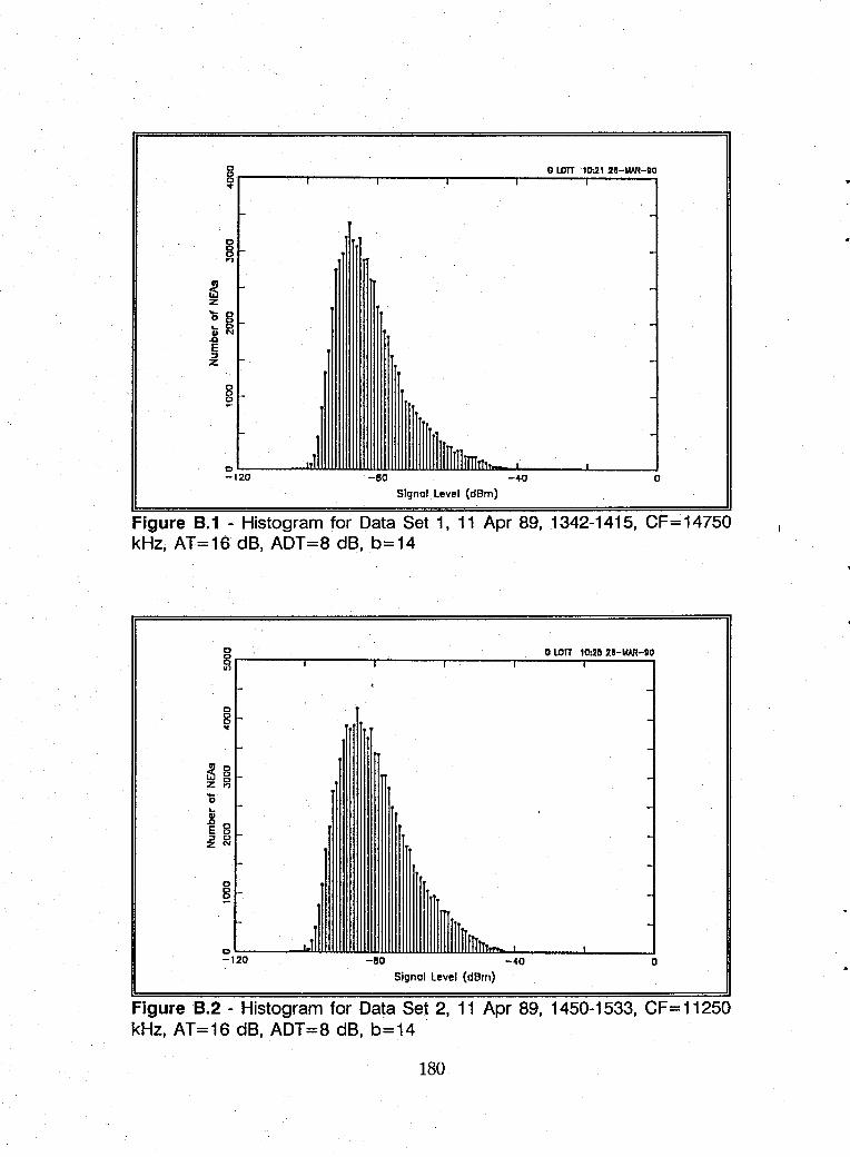
gr-____ -r ______ r-____ -r ______ r-~O~wrr~1~~~21~2e~-~Mm~-~DO !f I I

-

-

illllfrrlTITmnl. ~,·~20------~~WW~-~80~WW~~WW~--~~------L-I-----JO

-

Signal Level (dBm)

Figure B.1 - Histogram for Data Set 1,11 Apr 89,1342-1415, CF=14750 kHz, AT=16 dB, ADT=8 dB, b=14

o 0 LOTT 10:2D 2e-Mm-DO 8r------r------~----~------~~~~~~~ ~I

... II

o o o v

.Q 0 E 0 :J a ZN

Signal Level (dBm)

Figure B.2 - Histogram for Data Set 2, 11 Apr 89, 1450-1533, CF = 11250 kHz, AT=16 dB, ADT=8 dB, b=14

180

•

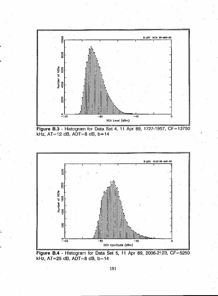
o lDTT 10:~1 2e-IM/I-IO 0 0 g ~

-0 g -III

-~ g Z g -'0 -L. .. .0 0 E 0

£ ~

0 0

~

0 IllllflrrTT~

-120 -BO -40 o NEA level (dBm)

Figure B.3 - Histogram for Data Set 4, 11 Apr 89, 1727-1957, CF=13750 kHz, AT=12 dB, ADT=8 dB, b=14

o ~r

o ~ -

~ Z 0

'O~ L. .. .0 E :J 0 Z g

g U)

o lDTT 10:33 28-1M/1-90 I T

.

-BO -40 o NEA Apmlltude (dBm)


181

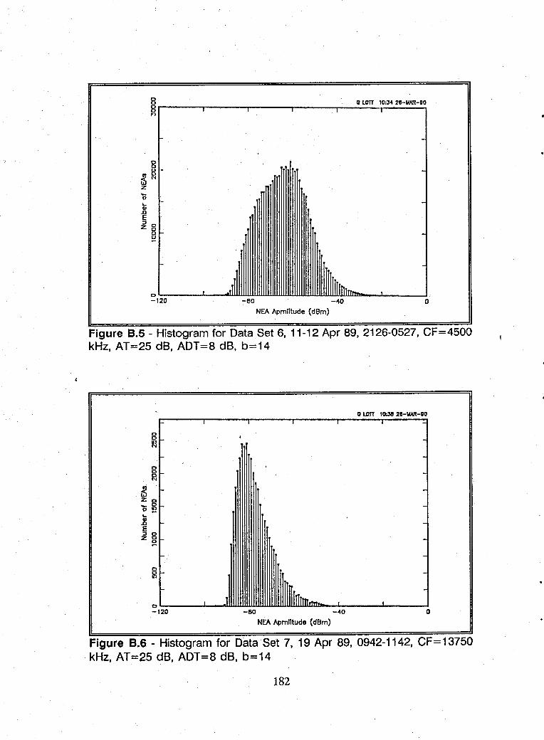
... CIJ .c E :f g

g

~1~2o~----~~~WJ~IWW_~eo~wmww~~lliWJilll_llillwrrn~ITh-~--~--__ ~O NEA Apmlltude (dBm)

Figure 8.5 - Histogram for Data Set 6, 11-12 Apr 89, 2126-0527, CF=4500 kHz, AT=25 dB, ADT=8 dB, b=14

~ z 0 .... 0 o ~ ... CIJ .c E ::l 0 zg

o LDTT lD:~ U-\AAR-ID T

J ,lmrrrfTTTrm I ~1~2~O----~--~ww_~eowwwwww~wm~-_~40------~-----Jo

NEA Apmlltude (dBm)


182

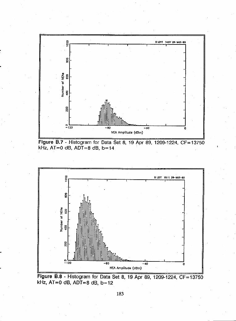
o 8r------r------.-----~------_r------r_~--_,

o 55

~8 z III

... CI

.1J E 0

£~

~1~20------~--ww~-~BWOillW~WW~~----~~------~----~0

NEA Amplitude (dl3m)

Figure B.7 - Histogram for Data Set 8, 19 Apr 89, 1209-1224, CF = 13750 kHz, AT=O dB, ADT=8 dB, b=14

o LOTT le:ll 20-UM-80 0 0

~ I I I

f- -0 0 III

~ 8 z ID

'0 ... -CI

.1J E 0 :J C Z ...

-o C -N -

ffimllJlrlTTT .....

- , C _,I

-I

-120 -BO -40 o NEA Amplitude (dBm)

Figure B.8 - Histogram for Data Set 8, 19 Apr 89, 1209-1224, CF = 13750 kHz, AT=O dB, ADT=8 dB, b=12

183

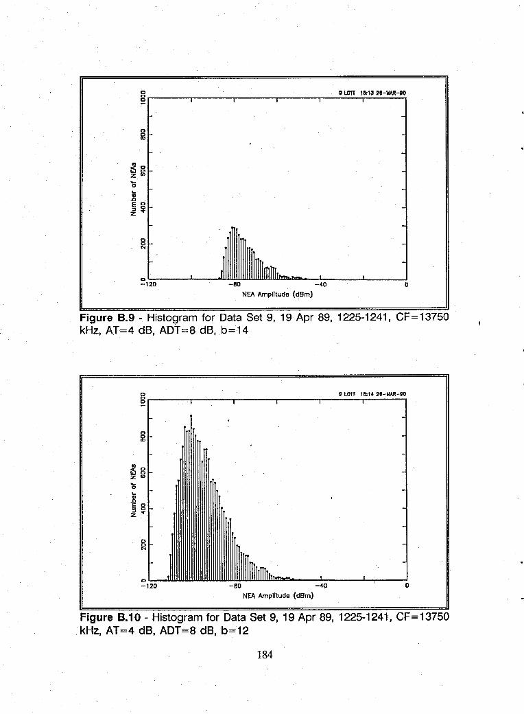
gr-____ -. ______ ~----_,------_r--~o~~~T'a;~1~~2~e-~WR~-ao

~8 z ID

L. II .0

§ ~ -z

~t~20~----~--~~-~B~0~Will~wm~~--~~~~----~-----J0

NEA Amplitude (dBm)


o lOTT le:t4 :l8-MAR-GO 0 0

~ I I I I I

-0 0 -IX)

~ 8 z ID

'0 -L. II .0 E 0

~~ -I- -

81-N

I-

0 -, I

-t20 -BO -w o NEA Amplitude (dBm)


184

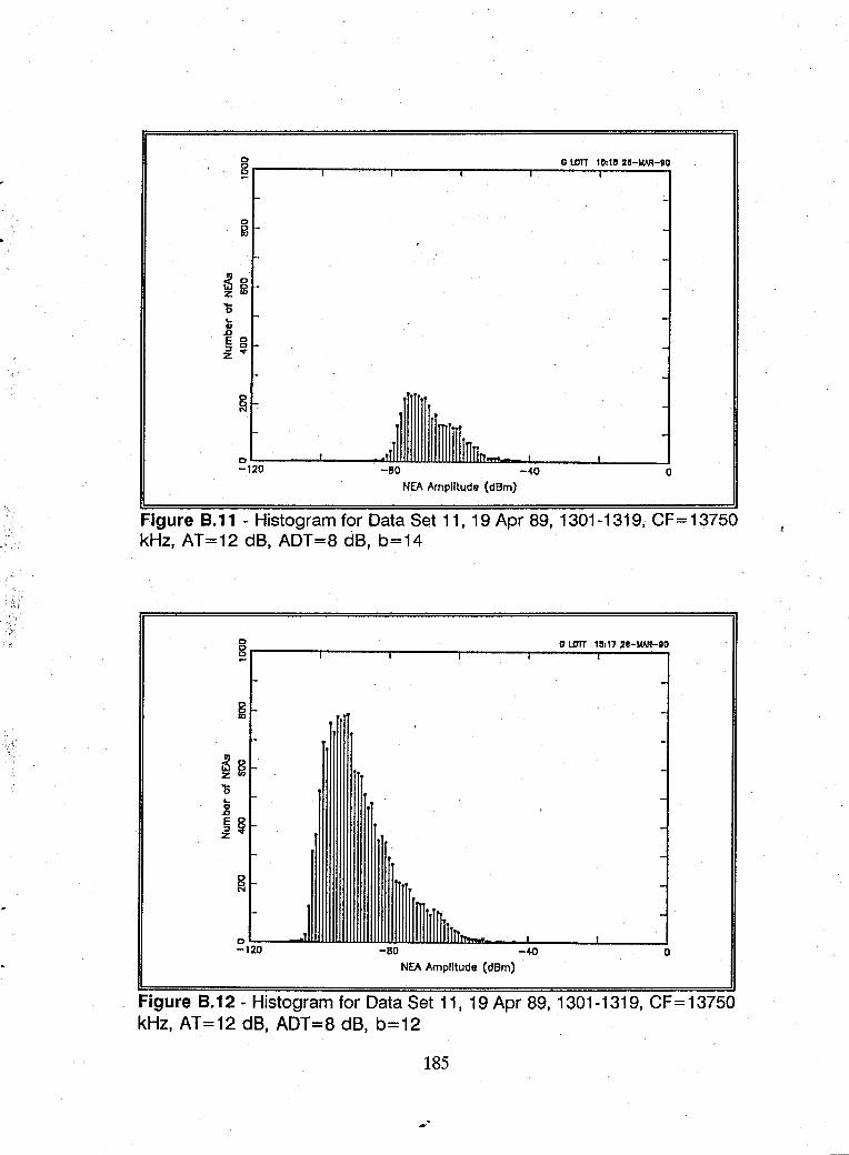
'i.

~1.';::20:;----'----~e~o WULWULlllW.W1U!moII-_L...40----ll...----l

0 NEA Amplitude (dBm)

Figure B.ll - Histogram for Data Set 11, 19 Apr 89, 1301-1319, CF = 13750 kHz, AT=12 dB, ADT=8 dB, b=14

o lDTT 111,1728-MAR-80 0 0 ~ I I I

0

16

-~ ~r -'0 r .. 1: ~ § z

0 0 N , 0

_,1 I -120 -eo -40 o

NEA Amplitude (dBm)


185

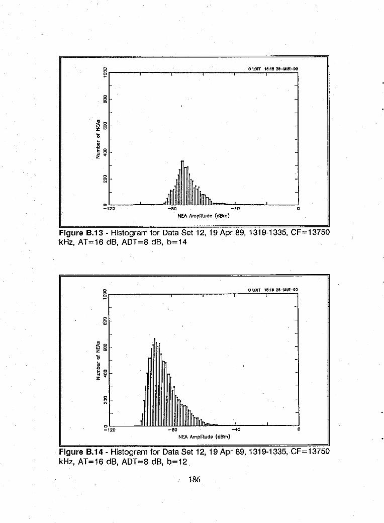
r:, 0 LOTT le:1!! 2e-MAR-DO gr------r------r------r------r-~~_r~~~

~8 z ID

... II

.D E 0 :l 0 Z ..,.

~ 1 .... 20---'-----n1lJ._8IlJ.OJJl.1ll"-llllWllLJJ.WJ~--_.l...40----"-----'O

NEA Amplitude (dBm)

Figure 8.13 - Histogram for Data Set 12, 19 Apr 89, 1319-1335, CF = 13750 kHz, AT=16 dB, ADT=8 dB, b=14

o 0 LOTT 111:111 2e-MAR-IIO 8r------r----r-----r----r-1-----r-,----~

-81-ID

I- -~8 z ID

'0 ... 1l E 0

~ 'Ii --

8 N

-ri IllllmllTT~ I oL-___ -WJJI.1lI"-llllWllLJJI.1lI~llJ.IlJ.wm~ ____ .!...-____ ~ __ ~

-120 -80 -40 0

NEA Amplitude (dBm)


186

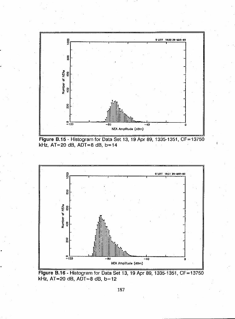
c o LOTT 111:20 28-WR-IO 0 CJ I -

-8 - -II>

-

~ ~ -'0 ... -II

.£I

E 8 £v

-0 CJ N

c _,11 IlmrlrJln ...

-120 -80 -40 0

NEA Amplitude (dBm)

Figure 8.15 - Histogram for Data Set 13,19 Apr 89,1335-1351, CF=13750 kHz, AT=20 dB, ADT=8 dB, b=14

o LOfT 1l),21 28-WR-1IO c 0 ~ I

-0 0 -II>

~ 0 z g '0 ... II .£I E 0 ::J 0 z v

-C 0 N

~ 1'::20:----L ... JolLWl.wwL.W1L_8~OJ.W.U.wIIL.W1LllrrrnLWJ.l1r"-----40'-----'----.lo NEA Amplitude (dBm)


187

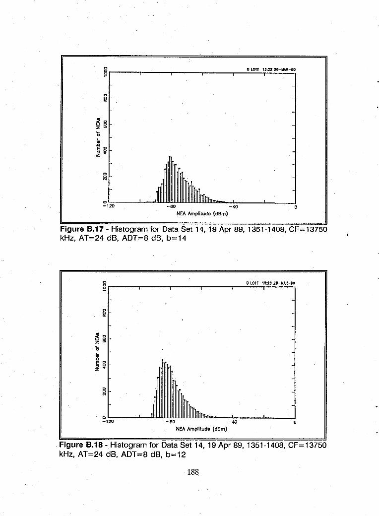
o C lDTT 18:22 28-\lAR-OO 8r------r------r------r----~~--~~~~~

~ 8-z w

~1~20~----~~www-~80~wmww~~~--~~------~----~O

NEA Amplitude (dBm)

Figure 8.17 - Histogram for Data Set 14, 19 Apr 89,1351-1408, CF=13750 kHz, AT=24 dB, ADT=8 dB, b=14

o C lDTT 18:23 n-\lAR-oo

8~----~------~----~------~-----r----~

~o z 16

~1~20~----.L..--uLw.w.W-~80.uWJw.w.WUlllJ.Ill----4.~-----J..-----JO

NEA Amplitude (dBm)


188

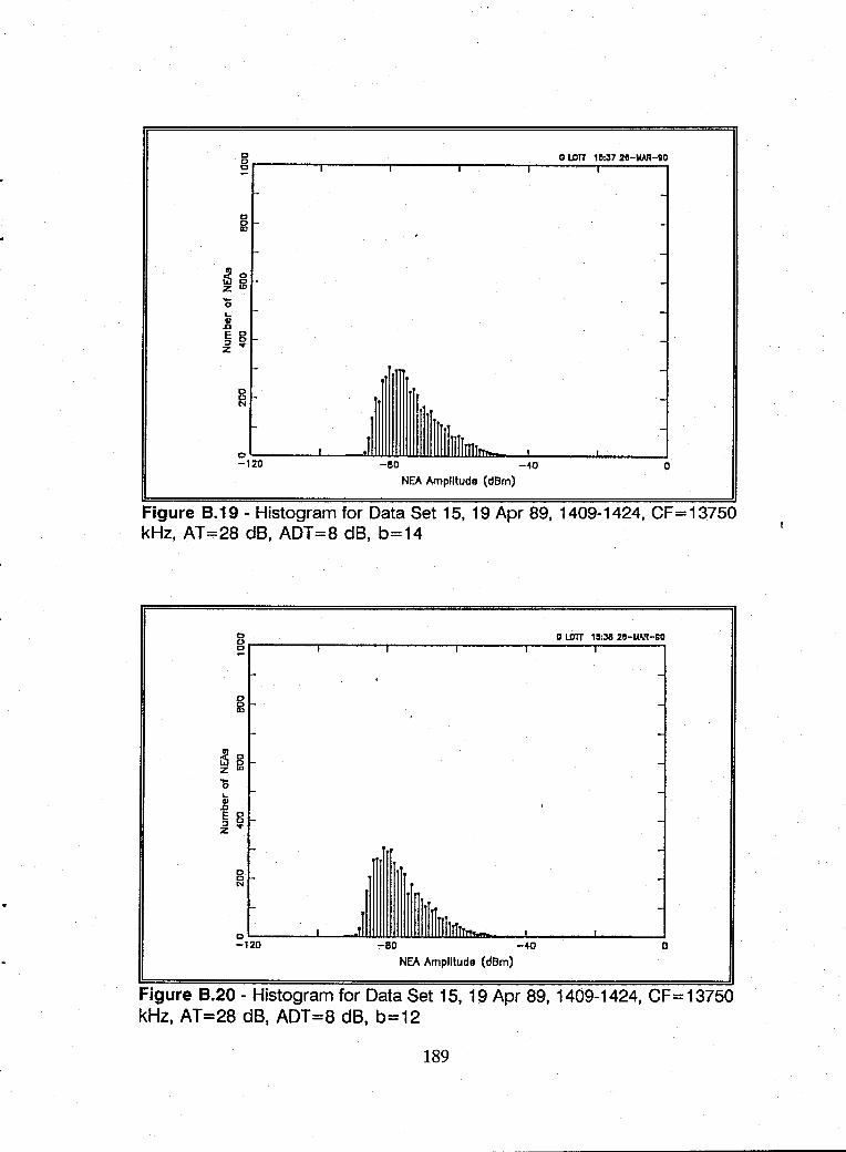
~8 z ID

'0 ... 1l E 8 ~ ...

~'~20~----~--~W_WBO~~WW~~---_~~------~----~O

NEA Amplitude (dBm)


0 o l.OTT 1!!:J8 2e-\Wl-90 0

~ I I I

I- ,

0 0 -II)

~ 8 z ID

'0 ... Q .c E 0 :l 0 Z ..,.

0 o -N

I Ilr~nhll~ 0 _,I

-120 -BO -~ 0

NEA Amplitude (dBm)


189

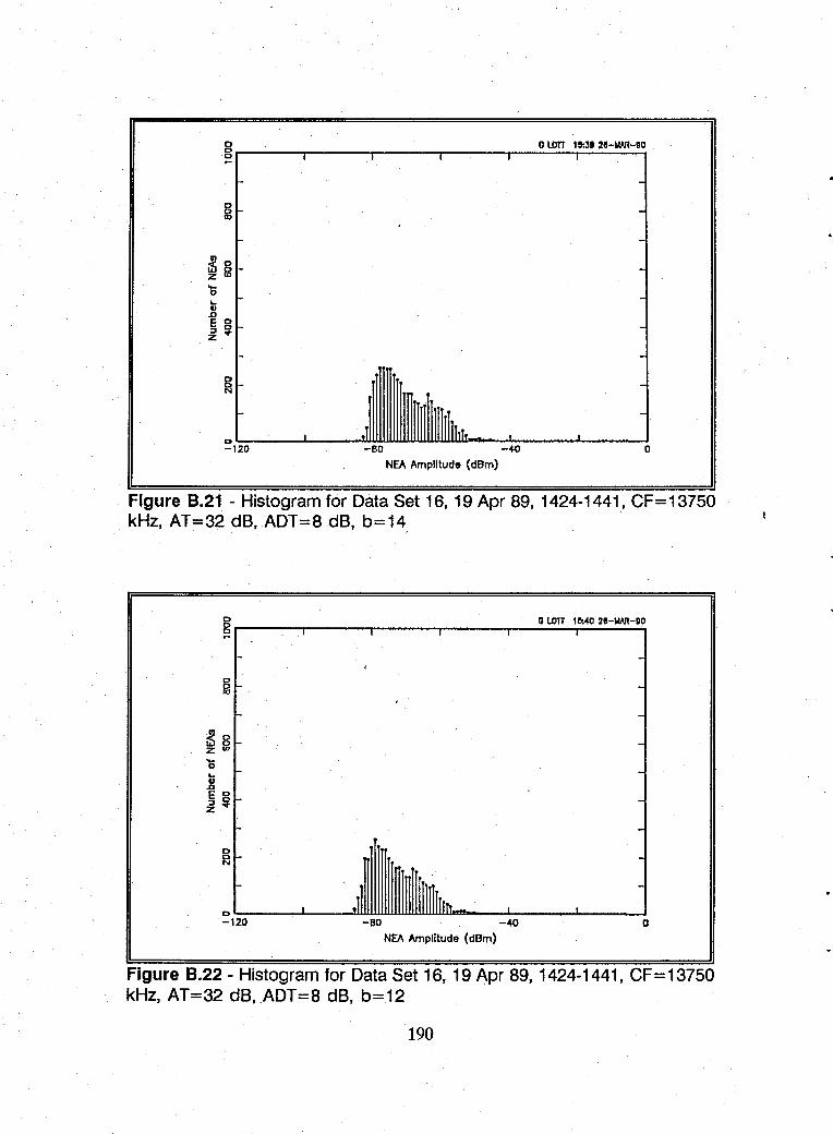
o 0 lO1T 1 1l:39 28-IoIAR-DO gr------r------r------r------r------r----~

L.. II ..0 E 0 :l 0 Z ..,.

D~ ____ ~ ____ -m~~wwmw~~ __ ~ ____ ~ ____ ~ -120 -BO --«) a

NEA Amplitude (dBm)


0 o lO1T 115:40 28-WJt-DO 0 0 I ~

I

-, 0 0 -ID

-~ g Zw -'0 L.. -II ..0 E 0 -:l 0 Z ..,.

-0 0 -N

, 1~llmhlfi. -

0 I _,11 _I _L

-120 -80 --«) 0 NEA Amplitude (dBm)


190

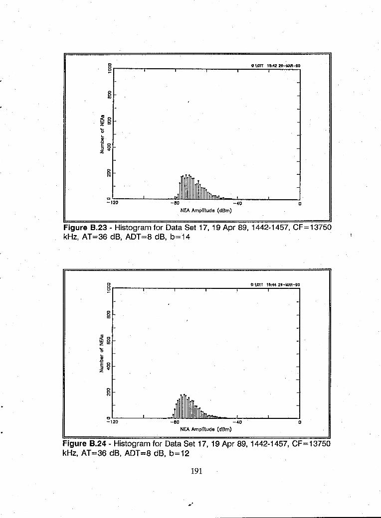
D o lO1T 1~:42 28-1AA/1-90 0 e I I

-D 0 II) -

-~8 z In -.... 0 .. 1/ .c E 0

~ ~

~

D J Illffillflm'T_. -120 -BO -40 0

NEA Amplitude (dBm)

Figure 8.23 - Histogram for Data Set 17,19 Apr 89, 1442-1457, CF=13750 kHz, AT=36 dB, ADT=8 dB, b=14

D 0 lO1T 111:44 28-1AA/1-90 g.------r------r------r------r---~~~~~

~ 0 z!6 '0 .. 1/ .c E D :l 0 Z ...

~,~20------~----~-wBO~~wwwm~----~W------~----~O

NEA Amplitude (dBm)


191

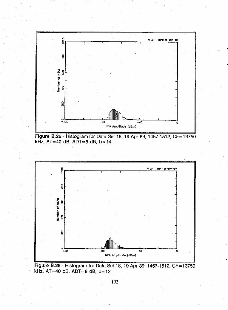
§r-____ -r ____ -. ______ ~----_.--~O=~~1~e:~~2e~-MAA~-OO

~1~20~--~~-----~8~0~wwwwwm-----~W------~--~0

NEA Amplitude (dBm)


o 0 LDTT 111:47 :ZO-MAA-SO g~----~----~------~----~--~~~~~

~g Z 10

L. 01

.fJ E g _ £ ....

o~ ____ -L _____ ~~illWillWmh~ __ ~ ______ ~ ____ ~

-120 -BO -4<) o NEA Amplitude (dBm)


192

.~.

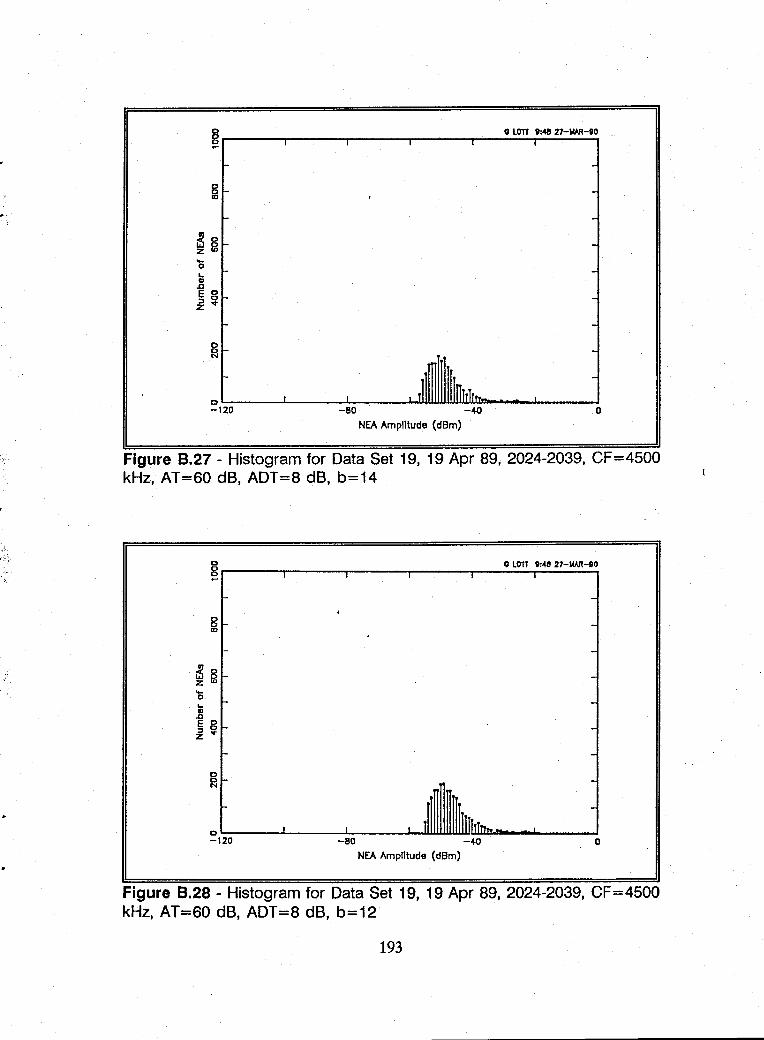
0 o LOTI ':48 27-IoIAR-eO 0 c I I I ~

g ,

~O Z ~ -'0 .. -CI .a

~ ~ -Z

-0 C -N

J11 IlfIITIT1TTT--

0 I -120 -BO -40 0

NEA Amplitude (dBm)

Figure B.27 - Histogram for Data Set 19, 19 Apr 89, 2024-2039, CF =4500 kHz, AT=60 dB, ADT=8 dB, b=14

0 o LOTI ':41! 27-IoIAR-BO 0 8 I I

, 0 0 ID

~8 z ID

'0 .. -CI

.D E 0 j C

Z ...

-0 C -N

Tfl lrIUI,Tn". -

0 I

-120 -BO -40 0 NEA Amplitude (dBm)


193

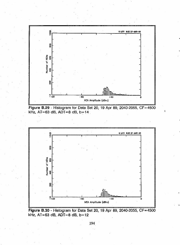
o gr------r------r------.------r-~~~~~~

~ 0 zl6 '0 ... 1l E g :f ...

~1~20~----~------~80------L-~IDW~-~Wmru~--~-----J0

NEA Amplitude (dBm)

Figure 8.29 - Histogram for Data Set 20, 19 Apr 89, 2040-2055, CF=4500 kHz, AT=63 dB, ADT=8 dB, b=:=14

c 0 LOfT ',iIJ 27-IMR-OO g~----_r------r-----_r------r-----_r----__,

~ 0 zl6 '0 ... IJ .0

~ ~ -z

cL-____ -L ______ L-____ -L-illWill~mm~ __ ~ ____ ~ -120 -BO -w o

NEA Amplitude (dBm)

Figure 8.30 - Histogram for Data Set 20, 19 Apr 89, 2040-2055, CF=4500 kHz, AT=63 dB, ADT=8 dB, b=12

194

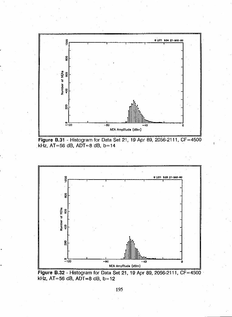
o LOTT 11:54 27-1oWt-;O 0 0 ~ I I

0

fi5

~8 z w

'0 ... .. .D E 0 :;, 0 z ..

-8 '"

0 I

1 rllllrnT~ -120 -BO -4C o

NEA Amplitude (dBm)


0 o LOTT 'II:1!a 27-1oWt-1IO 0 c I I ~

, -0

fi5 -

~o z III -0 ... .8 E 0 -:;, c Z ..

8 '"

0 I ,II l~lft'hT~. -120 -BO -40 0

NEA Amplitude (dBm)


195

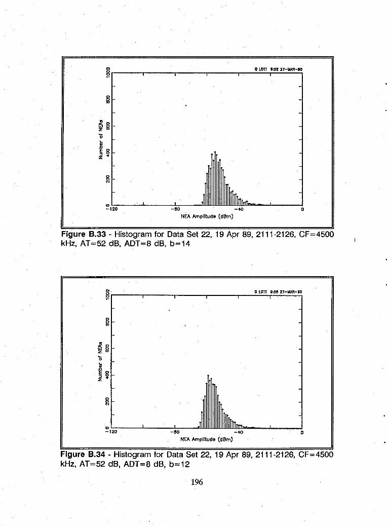
0 o lim ':118 27-WR-'O 0 ~

0

~ .

~g -Z ID

"-0 -.. .8 E g ~ .. -

-0 f;l -

1 Ir~lllnrn1. -c . .-'- I _,1 -120 -80 -4<) 0

NEA Amplitude (dBm)

Figure 8.33 - Histogram for Data Set 22, 19 Apr 89, 2111-2126, 'CF=4500 kHz, AT=52 dB, ADT=8 dB, b=14

0 o LorT D:I!S 27-WR-DO 0 ~ I

. -~ -

-~g -'0 ... -II .a

~ ~ -z

-0 f;l -

011 IlllirIrrTm~ -0 I I

-120 -80 -40 0

NEA Amplitude (dBm)

Figure 8.34 - Histogram for Data Set 22, 19 Apr 89, 2111-2126, CF =4500 kHz, AT=52 dB, ADT=8 dB, b=12

196

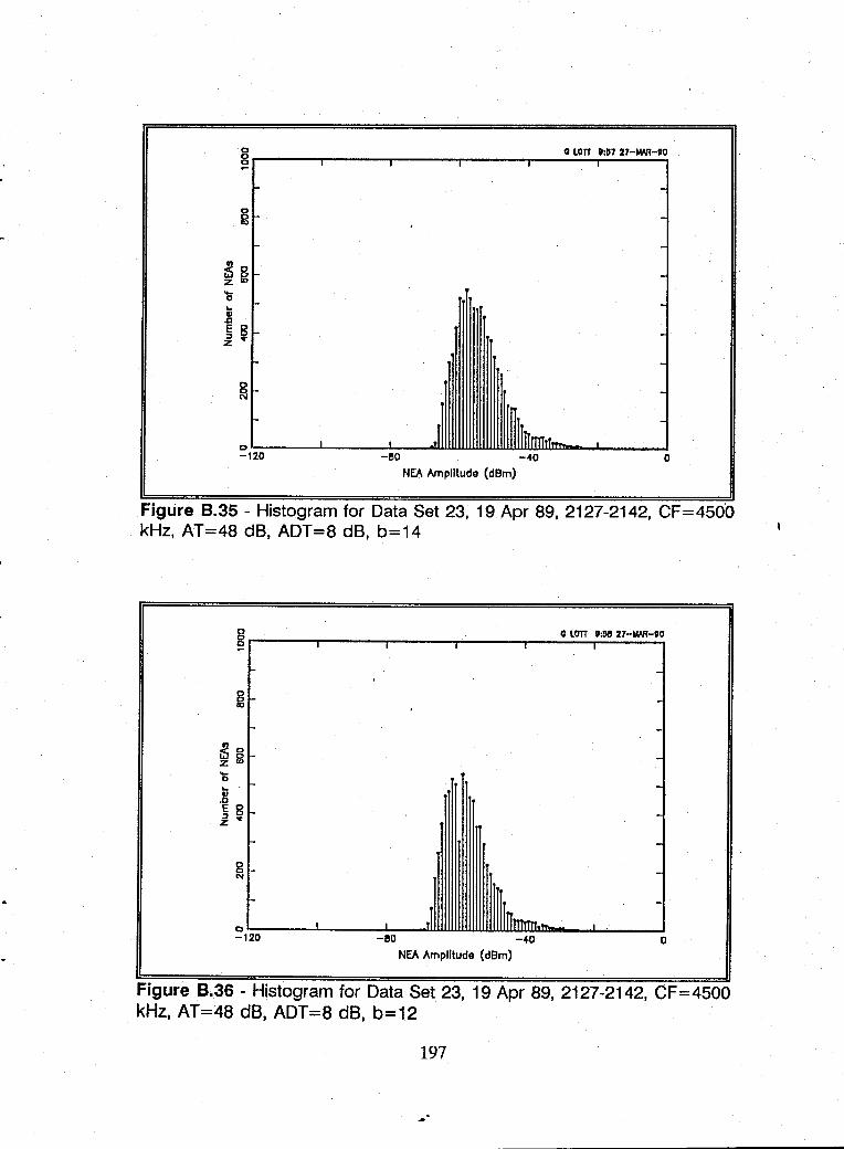
o 0 LOrr ',D7 27-IWI-IIO 8r-~--,-----~1------r-1-----,r-----~1------,

L.. II

.D E 0 ;;, 0 z ....

-BO -40

NEA Amplitude (dBm)

-

-

-

-

o

Figure B.35 - Histogram for Data Set 23, 19 Apr 89, 2127-2142, CF=450'O kHz, AT=48 dB, ADT=8 dB, b=14

0 o Lorr ',51! 27-UAR-OO 8 I I

-8 -OJ

r -~8 -z tD

'0 -L..

.8 ~ § f- -z

-8 -N

'r

_TJ Ilr ITTlTTTntth

-0

, , -120 -BO -40 0

NEA Amplitude (dBm)


197

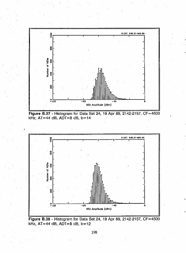
0 o tOil 11;511 27-\oIAR-1I0 0 !:! , , , ,

-gr- -

f- -~ 0 r-z 16 '0 r-.. 1l E 8 f-£~

0 C -N

0 I J IIllnrrTTTn. -T20 -BO -40 0

NEA Amplitude (dBm)


o 0 tOil 1I;1l1l 27-\oIAR-1I0

8~----~------~----~------~-----r----~ ~ "

-

-

.. 1l E 0

£~

-

-BO -.ro o NEA Amplitude (dBm)

Figure B.38 - Histogram for Data Set 24, 19 Apr 89,2142-2157, CF=4500 kHz, AT=44 dB"ADT=8 dB, b=12

198

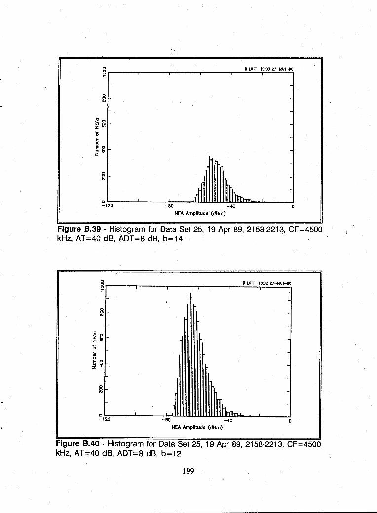
o 0 lDTT 10:00 27-MAR-DO gr-----~----~------~----_r--~~~~~ -

~ 0 z/6 '0 ... 1l § g z ...

~1~20~--~------_~e-o----~wmwmww_wwww~~~--~o

NEA Amplitude (dBm)


o lDTT 10:02 21-MAR-DO 0 0 ~ I

-gf- -

I- -~g z 10

'0 ... II .0 E 0

:£ ~

-0 0 N -

I- -I

0 I _.1 ~ I

-120 -eo -40 o NEA Amplitude (dBm)


199

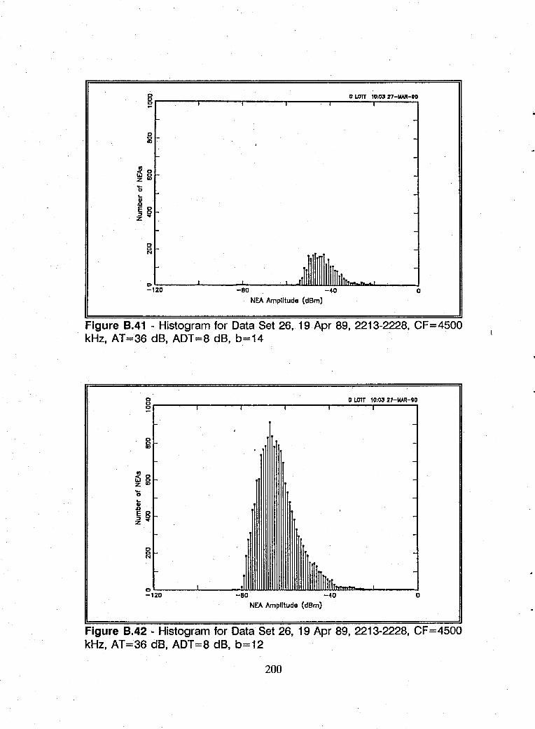
8~ ____ -r ______ ~ ____ ~ ______ ~~o~um~I~D~~27~-MM~-~OO

o oII>

~o z f6 b

~1~20~----L------_~eo------~~WWw_w~~~~~----~o

NEA Amplituda (dBm)


o 0 um 10:OJ 27-iAAR-OO g~----~------~----~------~~~-~I~~~

---

~g z '"

-b -.. .8 E 0

£!f --

-BO -40 o NEA Amplitude (dBm)


200

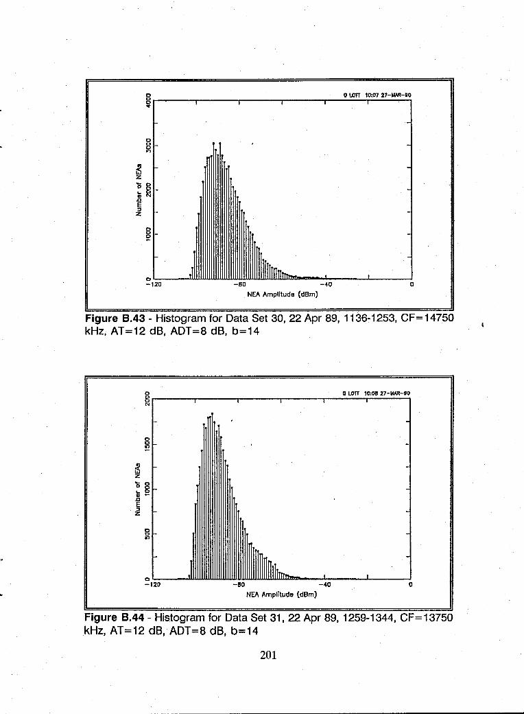
~~ ____ ~ ____ ~ ______ ~ ____ -r __ ~o~wrr 10:07 27-\Wt-aO -r

~ z '0 8 ... C II N .a E ;;J z

g -

-

-

-

-

I

-BO -40 0

NEA Amplitude (dBm)

Figure 8.43 - Histogram for Data Set 30, 22 Apr 89, 11 kHz, AT=12 dB, ADT=8 dB, b=14

36-1253, CF=14750

o owrr 8~----~----~------~----'~----N

~ z

~ § II .... .a E ;;J z

8 In

o~ __ ~~wmwmWillWillWIDwwmm~ __ ~ __ __ -120 -BO -40

NEA Amplitude (dBm)

Figure 8.44 - Histogram for Data Set 31, 22 Apr 89, 125 kHz, AT=12 dB, ADT=8 dB, b=14

201

10:011 27-\Wt-DO

--

-

-

--

I

0

9-1344, CF = 13750

..

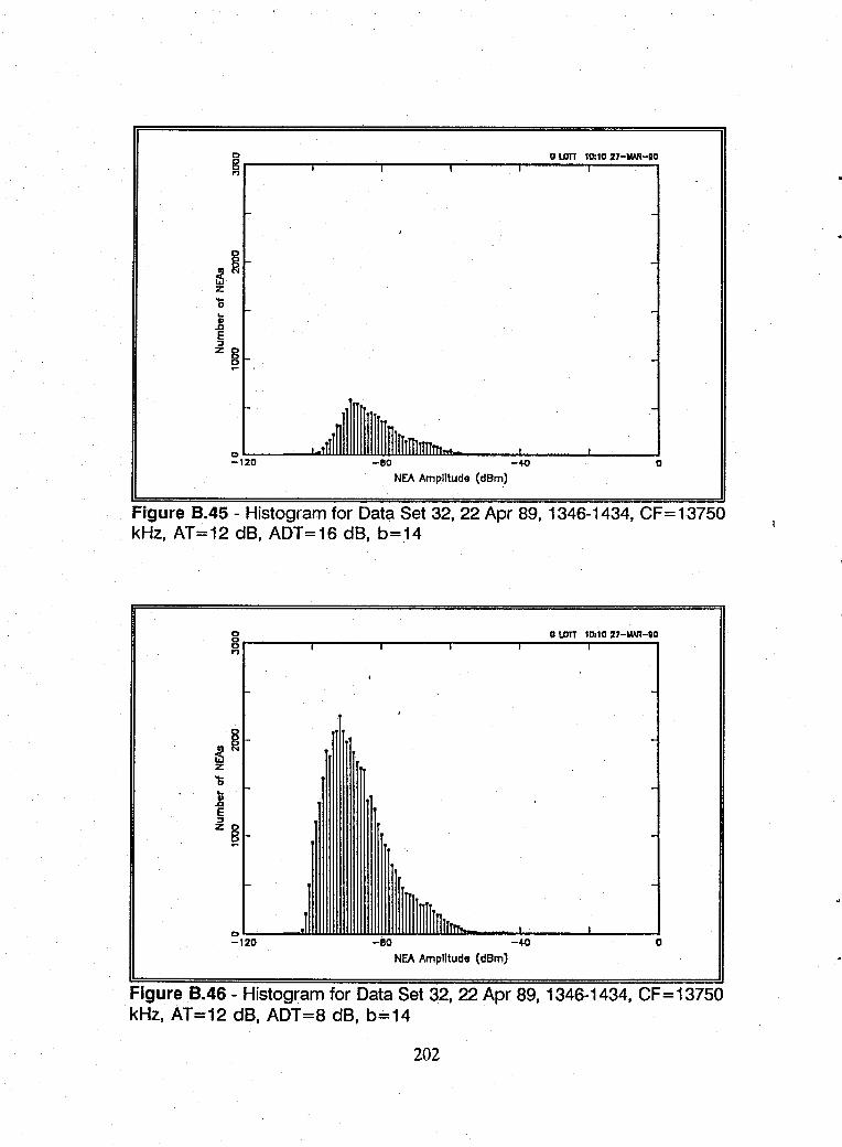
o OLDTT 10:10 27-1MR-IO ~r-----'-----~------~-----r----~r-----'

8 ~~ z '0 ... 1: E :J Z 8

o -

~'~20~--~~wwwm_meWomwlliW~------_~~------~------~O

NEA Amplitude (dBm)

Figure 8.45 - Histogram for Data Set 32, 22 Apr 89, 1346-1434, CF=13750 kHz, AT=12 dB, ADT=16 dB, b=.14

D 0 LDTT 10:10 27-1MR-IO g~----~----~------~-----r----~r-----' n

D~ ___ ~~WW~wmwmwwwwwm ____ ~ ______ ~ _____ ~ -120 -BO -4() 0

NEA Amplitude (dBm)


202

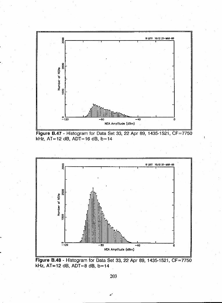
o 0 lD'IT 10:12 27-IWHIO R~----~----~------r-----~----~----~

-BO -40 o NEA Amplitude (dBm)


... .8 E ::I

8r-____ ,-____ ~------r_----_r--O~lD'IT~,I~~.1~22~7-~~~-gO ~) I I I

-

Z 0 8 -

-

~17.20~--~_~w,llwwwwww-~BO~~~~)ffi~TIrJ~~---~~----~I------Jo NEA Amplitude (dBm)


203

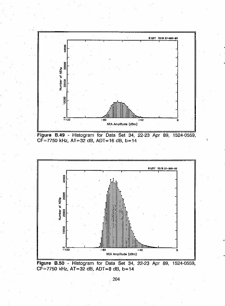
g 8 ~

-110 -40

NEA Amplitude (dBm)

o lDTT 10:111 27-IWHIO

o

Figure B.49 - Histogram for Data Set 34, 22-23 Apr 89, 1524-0559, CF=7750 kHz, AT=32 dB, ADT=16 dB, b=14

Figure B.50 - Histogram for Data Set 34, 22-23 Apr 89, 1524-0559, CF=7750 kHz, AT=32 dB, ADT=8 dB, b=14

204

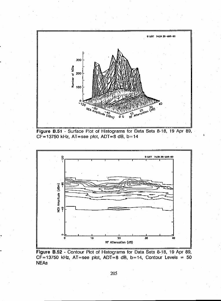
300

~ z '0 200

] § z 100

o lDTT 14:24 28-IoIAR-II0

Figure B.51 - Surface Plot of Histograms for Data Sets 8-18, 19 Apr 89, CF=13750 kHz, AT=see plot, ADT=8 dB, b=14

o 0 lDTT 14:;'11 28-IoIAR-OO ~r---~----~--~----~----~--~----~--~ I

o~ __ ~ ____ ~ __ ~ ____ ~ ____ ~ __ ~ ____ ~ __ ~ o w ~ ~

RF Attenuation (dB)

Figure B.52 - Contour Plot of Histograms for Data Sets 8-18, 19 Apr 89, CF=13750 kHz, AT=see plot, ADT=8 dB, b=14, Contour Levels = 50 NEAs

205

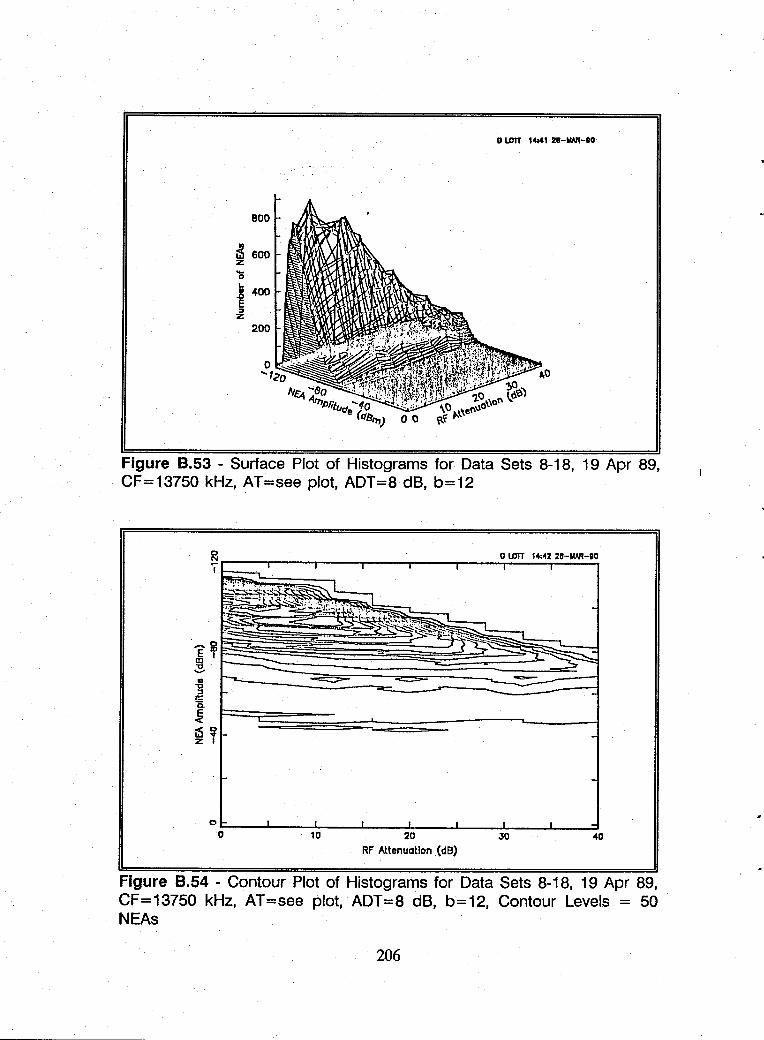
BOO

~ 600 z 'D .x 400 E :J

Z

200

o urn 14;41 28-ilAR-IO

Figure 8.53 - Surface Plot of Histograms for Data Sets 8-18, 19 Apr 89, CF=13750 kHz, AT=see plot, ADT=8 dB, b=12

o I.OlT 14;42 28-ilAR-DO

o~ __ ~ ____ ~ __ ~~ __ ~ ____ ~ __ ~ ____ ~ __ ~ o 10 20 3D 40

RF Attenuation (dB)

Figure 8.54 - Contour Plot of Histograms for Data Sets 8-18, 19 Apr 89, CF=13750 kHz, AT=see plot, ADT=8 dB, b=12, Contour Levels = 50 NEAs

206

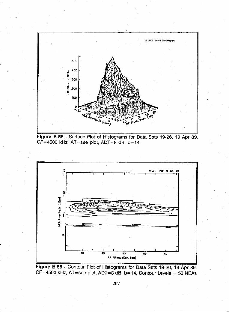
500

~ -400 z '0 300 .. 1l E 200 :J

Z

100

o IDlT 14<48 211-MAR-OO

Figure B.S5 - Surface Plot of Histograms for Data Sets 19-26, 19 Apr 89, CF=4500 kHz, AT=see plot, ADT=8 dB, b=14

o 0 IDlT 14;M 211-iAAR-OO 7,-~,--,-,--r---r-~r-~,r--',---,,---,,---~,--~,

o

-I I I I I I I I I

40 "" 50 55 60

RF Attenuation (dB)

Figure B.S6 - Contour Plot of Histograms for Data Sets 19-26, 19 Apr 89, CF=4500 kHz, AT=see plot, ADT=8 dB, b=14, Contour Levels = 50 NEAs

207

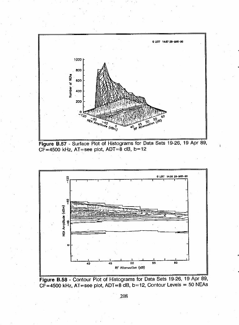
o LOTT 14:117 28-1oIAR-'O

1000

800

~ z 600 ~ "-II .a 400 E :> z

Figure B.57 - Suriace Plot of Histograms for Data Sets 19-26, 19 Apr 89, CF=4500 kHz, AT=see plot, ADT=8 dB, b=12

o LOTT 14:511 28-MAR-DO

0 IX> ,

E -. II) "0 ..... ., "0

,g~ c., .If is z

0

<40 45 50 55

RF Attenuat10n (dB)

Figure B.58 - Contour Plot of Histograms for Data Sets 19-26, 19 Apr 89, CF=4500 kHz, AT=see plot, ADT=8 dB, b=12, Contour Levels = 50 NEAs

208

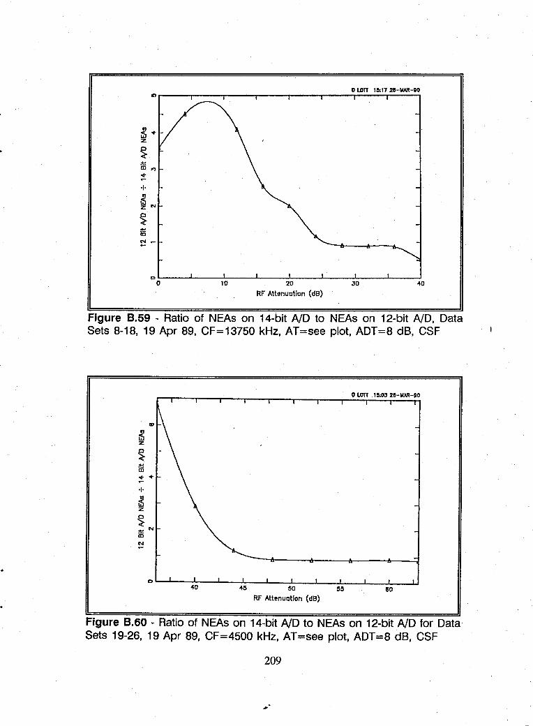
o lDTT 1e:17 2S-ioCAR-80

°O~--~--~1~O--~----~20----~--~----~--~40

RF Attenuation (dB)

Figure 8.59 - Ratio of NEAs on 14-bit NO to NEAs on 12-bit NO, Data Sets 8-18, 19 Apr 89, CF=13750 kHz, AT=see plot, ADT=8 dB, CSF

O~~~~~--~--~ __ ~ __ L-~~-L __ -L __ -U 40 45 50 55

RF Attenuation (dB)

Figure 8.60 - Ratio of NEAs on 14-bit NO to NEAs on 12-bit NO for Data Sets 19-26, 19 Apr 89, CF=4500 kHz, AT=see plot, ADT=8 dB, CSF

209

APPENDIX C

There are four main classifications of NO converters. These are:

• Servo or delta modulation

• Integrating or charge replacement

• Parallel threshold

• Successive approximation.

The earliest patent filing for a practical electronic NO converter was in 1948 for

an integrating type. There are many variations on these basic structures. This

appendix provides an overview of the basic types by combining descriptions from

multiple references. [Refs. 35,36,43,107,108]

Figure C.1 diagrams the structure of a servo or delta modulation type NO

converter. Upon each clock pulse, the counter counts up or down depending on

the difference between the input voltage and the output of the digital-to-analog

CD/A) converter. When the count stops, the counter output is the parallel

codeword for that voltage level. This converter scheme is most efficient for

monitoring a single signal, and it is simple to implement. The main disadvantage

is the slow conversion rate. For a 14-bit converter, conversion could require up

to. 16384 clock cycles. D/A errors will propagate through the system and appear

as codeword errors.

210

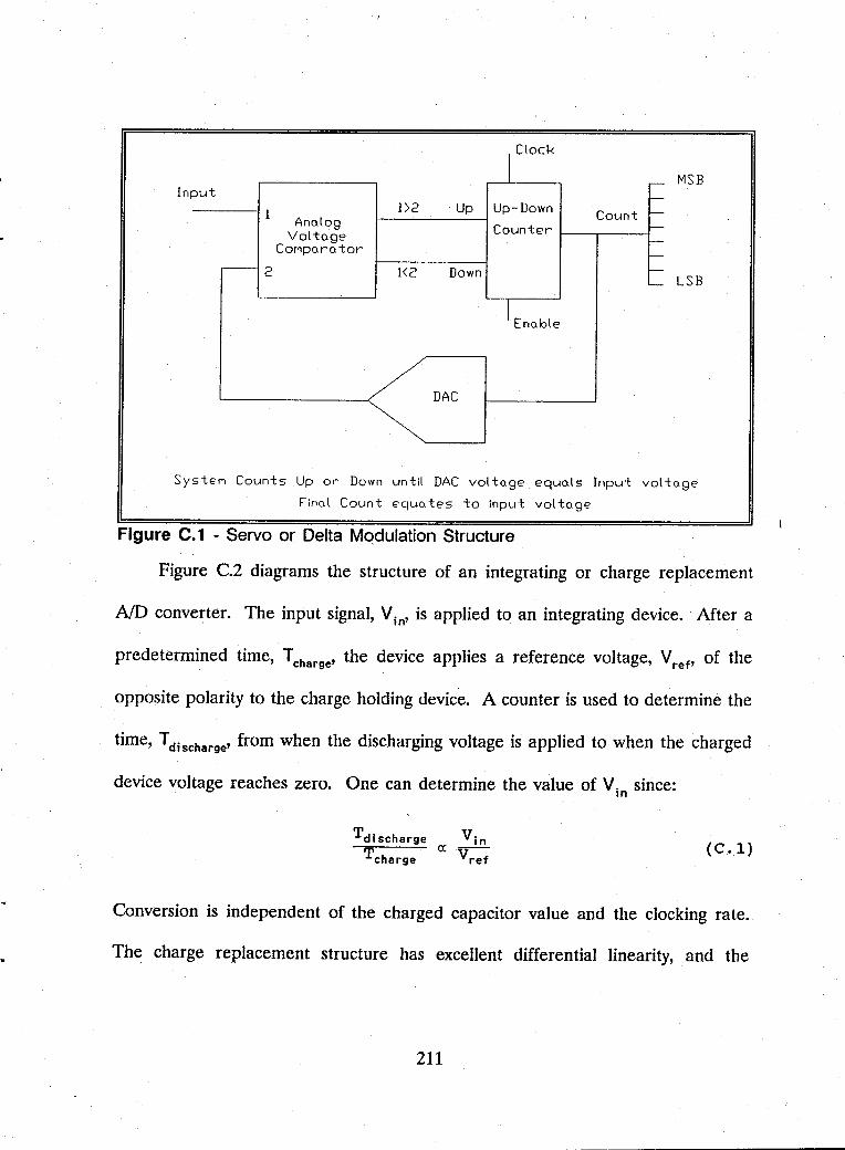
Clock

I r- MSB In put l-

I 1>2 Up Up-Down Count I-

Analog Counter r--Voltage r--

COMparator r--.---- 2 1<2 Down r-

~ LSB

I Eno.ble

DAC

SysteM Counts Up or Down until DAC vol to.ge equals Input voltage

Final Count equo.tes to input volto.ge

Figure C.1 - Servo or Delta Mqdulation Structure

Figure C.2 diagrams the structure of an integrating or charge replacement

NO converter. The input signal, Vin, is appJied to an integrating device. Mter a

predetermined time, T charge' the device appJies a reference voltage, V ref' of the

opposite polarity to the charge holding device. A counter is used to determine the

time, TdisCharge' from when the discharging voltage is appJied to when the charged

device voltage reaches zero. One can determine the value of V in since:

Tdischarge

Tcharge (C .1)

Conversion is independent of the charged capacitor value and the clocking rate.

The charge replacement structure has excellent differential linearity, and the

211

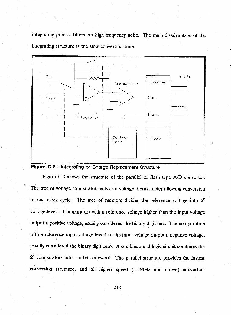
integrating process filters out high frequency noise. The main disadvantage of the

integrating structure is the slow conversion time.

L, Vin

I n bits

COMparator Counter

I I

Vref' Stop I

+ +

I I Start I Integra tor

I I I I L L _______ Control Clock Logic

Figure C.2 - Integrating or Charge Replacement Structure

Figure C.3 shows the structure of the parallel or flash type AID converter.

The tree of voltage comparators acts as a voltage thermometer allowing conversion

in one clock cycle. The tree of resistors divides the reference voltage into 2n

voltage -levels. Comparators with a reference voltage higher than the input voltage

output a positive voltage, usually considered the binary digit one. The comparators

with a reference input voltage less than the input voltage output a negative voltage,

usually considered the binary digit zero. A combinational logic circuit combines the

2" comparators into a n-bit codeword. The parallel structure provides the fastest

conversion structure, and all higher speed (1 MHz and above) converters

212

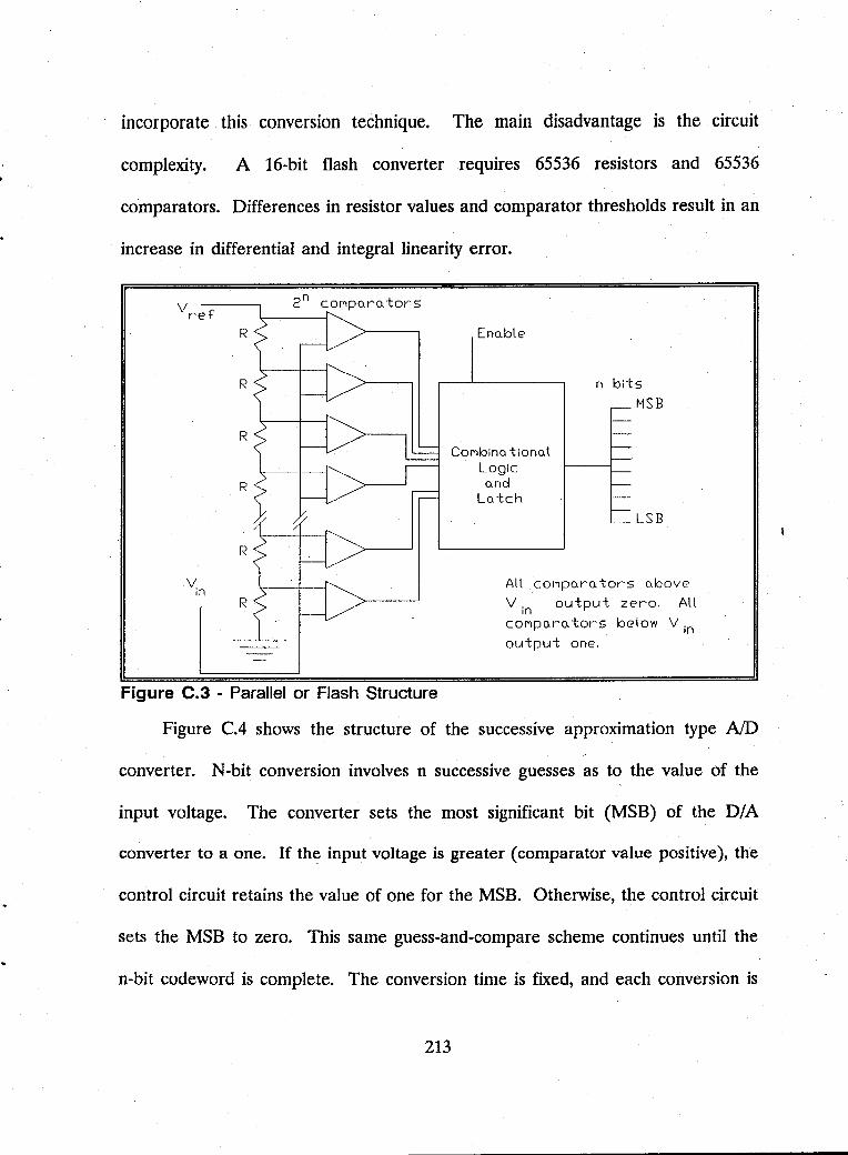
incorporate this conversion technique. The main disadvantage is the circuit

complexity. A 16-bit flash converter requires 65536 resistors and 65536

comparators. Differences in resistor values and comparator thresholds result in an

increase in diffe.rential and integral linearity error.

V ref R Eno.ble

R n bits MSB

R COl"lbina tiono.l

Logic R o.nd

Lo.tch LSB

R

Vin All cOl"lpo.ro.tors above R V, In output zero, All

cOMparators below V in output one,

Figure C.3 - Parallel or Flash Structure

Figure CA shows the structure of the successive approximation type NO

converter. N-bit conversion involves n successive guesses as to the value of the

input voltage. The converter sets the most significant bit (MSB) of the D/A

converter to a one. If the input voltage is greater (comparator value positive), the

control circuit retains the value of one for the MSB. Otherwise, the control circuit

sets the MSB to zero. This same guess-and-compare scheme continues until the

n-bit codeword is complete. The conversion time is fixed, and each conversion is

213

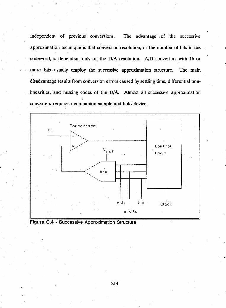
independent of previous conversions. The advantage of the successive

approximation technique is that conversion resolution, or the number of bits in the

codeword, is dependent only on the D/A resolution. AID converters with 16 or

more bits usually employ the successive approximation structure. The main

disadvantage results from conversion errors caused by settling time, differential non-

linearities, and missing codes of the D/A. Almost all successive approximation

converters require a companion sample-and-hold device.

V ln

COrlPQI~Q tor

~ .--V Control

V ref

I LogiC

D/A

Msb lsb ClOCK

n bits

Figure C.4 - Successive Approximation Structure

214

APPENDIX D

This appendix contains two work sheets developed using the IBM-PC software

MATHCAD, Ver. 2.5. The discussion about the systems modeled in the work

sheets is found in Chapter VIII.

215

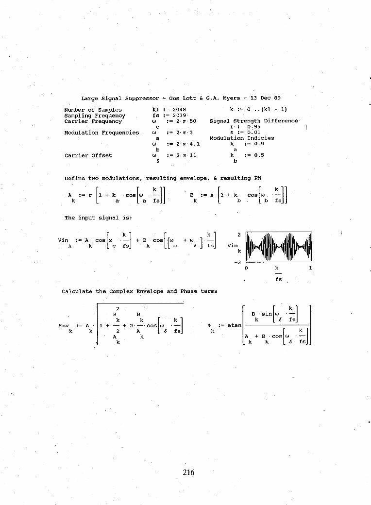
Large signal Suppressor - Gus Lett & G.A. Myers - 13 Dec 89

Number of Samples Sampling Frequency Carrier Frequency

Modulation Frequencies

carrier Offset

kl :=2048 fs := 2039 w := 2·.".·50

c w := 2·.".·3

a w := 2·",,·4.1

b w := 2·.".· 11

6

k := 0 .. (k1 - 1)

Signal Strength Difference r := 0.95 s := 0;01

Modulation Indicies k := 0.9

a k := 0.5

b

Define two modulations, resulting envelope, & resulting PM

The input signal is:

Calculate the Complex Envelope

2 B B k 2.~.COS[w Env := A· 1 + -+

k k 2 A 6 A k

k

and Phase terms

.~] 4> fs k

216

:=

2

vin k

-2

atan

0 k

fs

B .sin[w .~] k 6 fs

+ B . cos [(~ . ~] A k k 6 fs

1

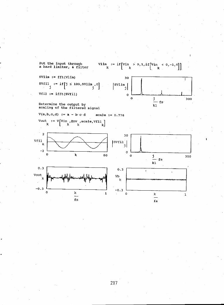
Put the input through a hard limiter, & filter

SVlim := fft(Vlim)

vlim k

SVfilj := if[j ~ lOO,SVlimj,O]

Vfil := ifft(SVfil)

Determine the output by scaling of the filtered signal

V(a,b,c,d) := a - b·c·d scale := 0.776

Vout := V[Vin ,Env ,scale,Vfil ] k k k k

o k 80

vo:~: ~ '~-~f4r'~ .) -0.3 - J

o k 1

fs

0.3

Vb k

-0.3

217

o j 300 _. fs kl

o j 300 _. fs kl

t·· ...... tI.\ .... ...... w .......

o k 1

fs

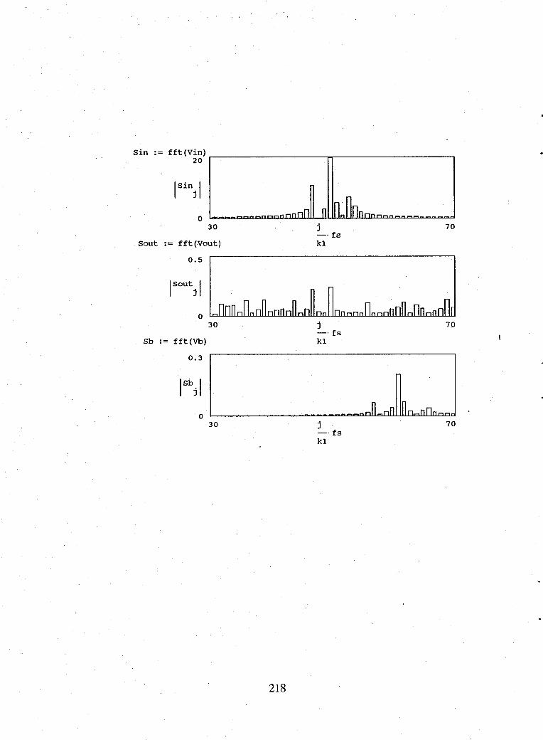
sin := fft(Vin) 20

ISinjl

0 30 j 70

_. fs " Sout := fft(Vout) kl

0.5

Isoutjl

0 30 j 70

_. fs Sb := fft(Vb) kl

0.3

ISbjl

0 30 j 70

_. fs kl

218

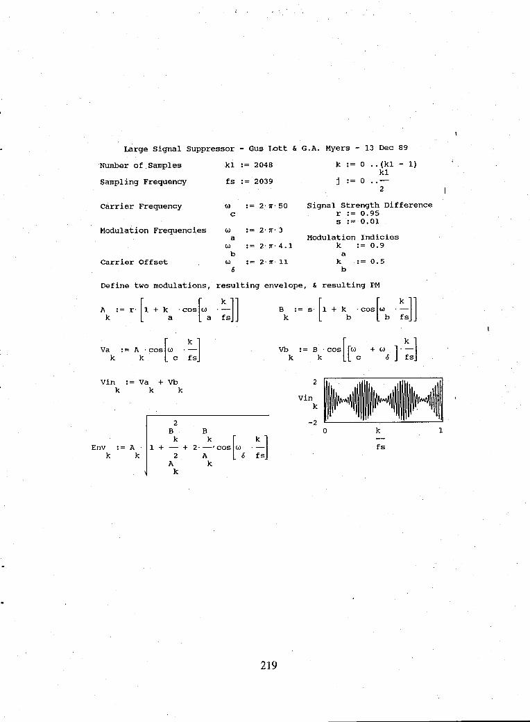
Large Signal Suppressor - Gus Lott & G.A. Myers - 13 Dec 89

Number of Samples k1 := 2048 k := 0 •• (k1 - 1) k1

Sampling Frequency fs := 2039 j := 0 2

Carrier Frequency W := 2'7r'50 Signal strength Difference c r := 0.95

s := 0.01 Modulation Frequencies W := 2'7r'3

a Modulation Indicies W := 2'7r'4.1 k := 0.9

b a Carrier Offset W := 2'7r'11 k := 0.5

6 b

Define two modulations, resulting envelope, & resulting PM

A := r' [1 + k ,cos[W ' :s]] k a a

B := s' [1 +kb

'cos[Wb ' :J] k

Va := A ,cos[W ' :s] k k C

Vb := B k' cos [ [(,) C + (,) ], :J k 6

Vin := Va + Vb 2 k k k

Vin k

2 -2 B B 0 k 1

k 2'~'COS[(') ,~] Env := A, 1 + - + k k 2 A 6 fs

fs

A k k

219

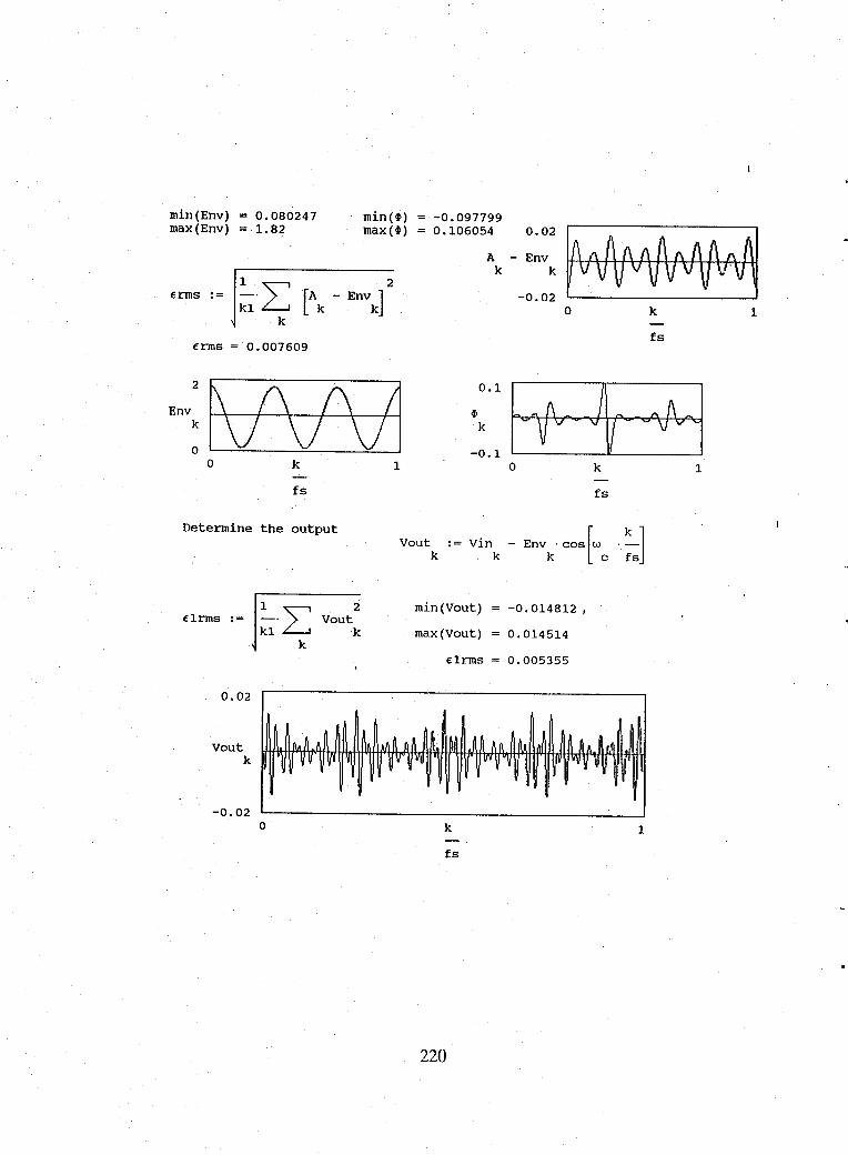
min(Env) max (Env)

0.080247 1.82

fnns = 0.007609

o k

fs

Detennine the output

1 f1nns :=

k1°L: Vout

k

0.02

Vout k

-0.02 0

min (it) max(it)

1

2

k

-0.097799 0.106054 0.02

A - Env k k

-0.02 o

0.1

-0.1 o

min (Vout) -0.014812 I

max (Vout) 0.014514

f1nns 0.005355

k

fs

k

fs

k 1

fs

220

1

1

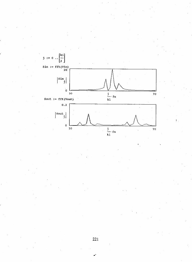
j := 0 .. [:1] Sin := fft(Vin)

20

/Sin j /

0 30

Sout := fft(Vout)

0.2

/SOU\/

0 30

221

j -. fs k1

j -. fs k1

70

70

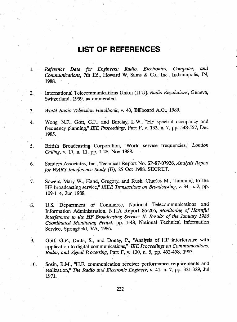
LIST OF REFERENCES

1. Reference Data for Engineers: Radio, Electronics, Computer, and Communications, 7th Ed., Howard W. Sams & Co., Inc., Indianapolis, IN, 1988.

2. International Telecommunications Union (ITU), Radio Regulations, Geneva, Switzerland, 1959, as ammended.

3. World Radio Television Handbook, v. 43, Billboard A.G., 1989.

4. Wong, N.F., Gott, G.F., and Barclay, L.W., "HF spectral occupancy and frequency planning," lEE Proceedings, Part F, v. 132, n. 7, pp. 548-557, Dec 1985.

5. British Broadcasting Corporation, "World service frequencies," London Calling, v. 17, n. 11, pp. 1-28, Nov 1988.

6. Sanders Associates, Inc., Technical Report No. SP-87-07926, Analysis Report for WARS Interference Study (U), 25 Oct 1988. SECRET.

7. Sowers, Mary W., Hand, Gregory, and Rush, Charles M., "Jamming to the HF broadcasting service," IEEE Transactions on Broadcasting, v. 34, n. 2, pp. 109-114, Jun 1988.

8. U$. Department of Commerce, National Telecommunications and Information Administration, NTIA Report 86-206, Monitoring of Harmful Interference to the HF Broadcasting Service: II Results of the January 1986 Coordinated Monitoring Period, pp. 1-48, National Technical Information Service, Springfield, VA, 1986.

9. Gott, G.F., Dutta, S., and Donay, P., "Analysis of HF interference with application to digital communications," lEE Proceedings on Communications, Radar, and Signal Processing, Part F, v. 130, n. 5, pp. 452-458, 1983.

10. Sosin, B.M., "H.F. communication receiver performance requirements and realization," The Radio and Electronic Engineer, v. 41, n. 7, pp. 321-329, Jul 1971.

222

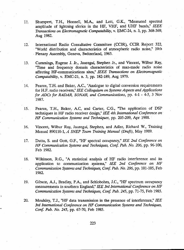
11. Shumpert, T.H., Honnell, M.A, and Lott, G.K., "Measured spectral amplitude of lightning sferics in the HF, VHF, and UHF bands," IEEE Transactions on Electromagnetic Compatability, v. EMC-24, n. 3, pp. 368-369, Aug 1982.

12. International Radio Consultative Committee (CCIR), CCIR Report 322, "World distribution and characteristics of atmospheric radio noise," 10th

. Plenary Assembly, Geneva, Switzerland, 1963.

13. Cummings, Eugene J. Jr., Jauregui, Stephen Jr., and Vincent, Wilbur Ray, ''Time and frequency domain characteristics of man-made radio noise affecting HF-communications sites," IEEE Transactions on Electromagnetic Compatability, v. EMC-21, n. 3, pp. 182-189, Aug 1979.

14. Pearce, T.H. and Baker, A.C., "Analogue to digital conversion requirements for H.F. radio receivers," lEE Colloquium on Systems Aspects and Applications for ADCs for RADAR, SONAR, and Communications, pp. 4-1 - 4-5, 3 Nov 1987.

15. Pearce, T.H., Baker, A.C, and Carter, c.G., "The application of DSP techniques in HF radio receiver design," lEE 4th International Conference on HF Communication Systems and Techniques, pp. 205-209, Apr 1988.

16. Vincent, Wilbur Ray, Jauregui, Stephen, and Adler, Richard W., Training Manual 890110-1, A SNEP Team Training Manual (Draft), May 1989.

17. Dutta, S. and Gott, G.F., "HF spectral occupancy," lEE 2nd Conference on HF Communication Systems and Techniques, Conf. Pub. No. 206, pp. 96-100, Feb 1982.

18. Wilkinson, R.G., "A statistical analysis of HF radio interference and its application to communication systems," lEE 2nd Conference on HF Communication Systems and Techniques, Conf. Pub. No. 206, pp. 101-105, Feb 1982.

19. Gibson, A.J., Bradley, P.A., and Schlobohm, J.c., "HF spectrum occupancy measurements in southern England," lEE 3rd International Conference on HF Communication Systems and Techniques, Conf. Pub. 245, pp. 71-75, Feb 1985.

20. Moulsley, T.J., "HF data transmission in the presence of interference," lEE 3rd International Conference on HF Communication Systems and Techniques, Conf. Pub. No. 245, pp. 67-70, Feb 1985.

223

21. Gibson, A.J. and Arnett, L., "New HF spectrum occupancy measurements in southern England," lEE 4th International Conference on HF Radio Systems and Techniques, Conf Pub. No. 284, pp. 159-164, Apr 1988.

22. Laycock, P.J. and others, "A model for HF spectral occupancy," lEE 4th International Conference on HF Communication Systems and Techniques, Conf. Pub. No. 284, pp. 165-171, Apr 1988.

23. Perry, B.D, and Abraham, L.G., "A wideband HF interference and noise model based on measured data," lEE 4th International Conference on HF Communication Systems and Techniques, pp. 172-176, Apr 1988.

24. Hagn, George H., Stehle, Roy H., and Harnish, Lawrence 0., "Shortwave broadcasting band spectrum occupancy and signal levels in the continental United States and western Europe," IEEE Transactions on Broadcasting, v. 34, n. 2, pp. 115-125, Jun 1988.

25. Aitchison, J. and Brown, J.A.C., The Lognormal Distribution, Cambridge University Press, London, 1957.

26. Croxton, Fredrick E., Cowden, Dudley J., Klein, Sidney, Applied General Statistics, 3rd Ed., Prentice-Hall, Englewood Cliffs, NJ, 1967.

27. Sachs, Lothar, Applied Statistics, a Handbook of Techniques, 5th Ed., Springer-Verlag, NY, 1982.

28. Hart, William C. and Malone, Edgar W., Lightning and Lightning Protection, Don White Consultants, Inc., Gainnesville, VA, 1979.

29. Maslin, Nicholas M., HF Communications: A Systems Approach, Plenum Press, NY, 1987.

30. Ziemer, Rodger E. and Peterson, Roger L., Digital Communications and Spread Spectrum Systems, Macmillan Publishing Co., NY, 1985.·

31. IWG Corp. Report IWG-FR-087-12, Operators Manual for the United States Coast Guard Advanced PROPHET System, prepared for Naval Ocean Systems Center (Code 542), San Diego, CA, pp. 96-102,201-202, 1 Nov 1987.

32. Harthcock, Clyde T.,An Examination of the Radio Frequency Switching Matrix at U.S. Army Field Station Augsburg, U.S. Army Field Station Berlin, and U.S. Naval Security Group Activity Edzell, Master's Thesis, Naval Postgraduate School, Monterey, CA, Sep 1989.

224

33. Hurley, J.M. Jr., HF Digital Subcarrier Receiver System, Master's Thesis, Naval Postgraduate School, Monterey, CA, Dec 1985.

34. Carson, M.H., Consideration for an All-Digital HFDF System, Master's Thesis, Naval Postgraduate School, Monterey, CA, Dec 1982.

35. Jenkins, A., "D-A and A-D conversion," Microelectronics and Reliability, v.21, n. 3, pp. 329-341, 1981.

36. Gordon, Bernard M., "Linear electronic analog/digital conversion architectures, their origins, parameters, limitations, and applications," IEEE Transactions on Circuits and Systems, v. CAS-25, pp. 391-418, Jul 1978.

37. Schweber, B. and Labs, W., "AID converters: 16-bit resolution isn't always enough," Chilton's IC&S (USA), v. 61, n. 2, pp. 51-52, Feb 1988.

38. Little, AI and Burnett, Bob, "S/H amp-ADC matrimony provides accurate sampling," EDN, v. 33, n. 3, pp. 153-166, 4 Feb 1988.

39. Tewksbury, Stuart K. and others, "Terminology related to the performance of S/H, AID, and D/A circuits," IEEE Transactions on Circuits and Systems, v. CAS-25, pp. 419-426, Jul 1978.

40. Brigham, E.O. and Cecchini, L.R., "A nomogram for determining FFT system dynamic range," Proceedings of the IEEE International Conference on Acoustics, Speech, and Signal Processing, Hartford, CT, pp. 623-627, 9-11 May 1977.

41. Doernberg, Joey, Lee, Hae-Seung, and Hodges, David A., "Full-speed testing of AID converters," IEEE Journal of Solid-State Circuits, v. SC-19, n. 6, pp. 820-827, Dec 1984.

42. Naylor, Jim R., "Testing digital/analog and analog/digital converters," IEEE Transactions on Circuits and Systems, v. CAS-25, pp. 526-538, Jul 1978.

43. Sheingold, D.H., Analog-Digital Conversion Hankbook, Analog Devices, Inc., 1972.

44. Aiken Advanced Systems, Technical Note SDS-101, Output Intercept Point Calculations, pp. 1-4, not dated.

225

45. Steinbrecher, Donald H., "Fundamental limitations on Accuverter performance," unpublished internal Steinbrecher Corporation, Woburn, MA, paper discussed with author during interview at the Naval Postgraduate School, Monterey, CA, on 4 Nov 1988.

46. Gray, G.A. and Zeoli, G.W., "Quantization and saturation noise due to analog-to-digital conversion," IEEE Transactions on Aerospace and Electronic Systems, Jan 1971.

47. Gaskell, P.S., "Evaluating ADC's for zero-IF digital radios," lEE Colloquium on Systems Aspects and Applications of ADC's for RADAR, SONAR, and Communications, pp. 5-1 - 5-4, 3 Nov 1987.

48. Anderson, D.T. and Whikehart, "A digital signal processing HF receiver," lEE 3rd International Conference on HF Communication Systems and TechnUjues, Conf. Pub. No. 245, pp. 89-93, Feb 1985.

49. Ghausi, M.S. and Laker, K.R.; Modern FilterDesign, Prentice-Hall, 1981.

50. Morgan, S. Kent, "Modem dataaquisition is complex," Electronic Design, v. 22, pp. 60-66, 25 Oct 1977.

51. Harris, F.J., "On the use of windows for harmonic analysis with the discrete Fourier transform," IEEE Proceedings, v. 66, n. 1, pp. 51-83, Jan 1978.

52. Oppenheim, A.V. and Weinstein, C.J., "Effects of finite register length in digital filtering and fast Fourier transform," IEEE Proceedings, v. 60, n. 8, pp. 957-976, Aug 1972.

53. Welch, Peter D., "A fixed point fast Fourier transform error analysis," IEEE Transaction on Audio and Electroacoustics, pp. 151-157, Jun 1969.

54. Tarver, Raymond J., "Graphs aid selection of A-D converters," Electronics, v. 47, n. 4, pp.ll0-ll1, 21 Feb 1974.

55. Hariharan, P.R., "Note on dynamic range of quantizers," IEEE Transactions on Aerospace and Electronic Systems, v. AES-5, n. 5, pp. 875-877, 5 Sep 1969.

56. Fogarty, John D., "Know your AID converter's dynamic range," Electronic Design, v. 23, n. 3, pp. 76-78, 1 Feb 1975.

226

•

57. Labutin, V.K., "Nomogram for finding the parameters of an analog-digital signal converter," Telecommunications and Radio Engineering, v. 35-36, n. 3, pp. 108-109, Mar 1981.

58. Story, M.J., "Hardware costs of systems aspects of ADCS," lEE Colloquium on Systems Aspects and Applications of ADCs for RADAR, SONAR, and Communications, pp. 1-1 - 1-9, 3 Nov 1987.

59. deGraaf, K., Air Force Wright Aeronautical Laboratories, Technical Report AFW AL-TR-83-1090, High Speed AID Converter Development Phase I, Jun 1983.

60. Burr-Brown Inc., Technical Data Sheet ADC600, 12-Bit Ultra-High Speed AID Converter, pp. 1-18, 1987.

61. Albaugh, Neil, "New ADCs for RF signal processing," RF Design, v. 10, n. 12, pp. 33-38, Nov 1987.

62. Breed, G.A. "High speed NO and DIA conversion," RF Design, v. 11, n. 1, pp. 39-40, Jan 1988.

63. Muto, Arthur S., Peetz, Bruce E., and Rehner, Robert c., "Designing a tenbit, twenty-megasample-per-second analog-to-digital converter system," Hewlett-Packard Journal, v. 33, n. 11, pp. 9-20, Nov 1982.

64. Burr-Brown Inc., Advance Technical Data Sheet ADC70l/SHC702, High Speed 16-bit Sampling AID Converter System, p. 1, Dec 1987.

65. Althouse, E.L., Mesias, S., and Kopp, D.M., Naval Research Laboratory, Memorandum Report 5518, The Use of a High-Speed 12-bit AID Converter for Digital Sampling of Communication Signal Carriers, 31 Dec 1984.

66. Bagwell, D.J. and Considine, V., "Digital processing architectures for HF radio receivers," lEE 3rd International Conference on HF Communication Systems and Techniques, Conf. Pub. No. 245, pp. 86-88, Feb 1985.

67. Burrier, Richard and others, "Floating-point converter used hardware to get a 20-bit dynamic range," Electronic Design, v. 32, n. 18, pp. 175-186, 6 Sep 1984.

68 . Davies, Kirk E., Floating-Point AID and DIA Converter, U.S. Patent 4,393,369, 12 Jul 1983.

227

69. Lacy, James and McMullin, Finbarr, "Enhancing the dynamic range of an AID converter," Electronic Engineering (GB) , v. 55, n. 680, pp.49-52, Aug 1983.

70. Nguyen, Chieu, "Digital autQmatic level control for analog-to-digital conversion," paper presented at the 76th Convention of the Audio Engineering Society, New York City, NY, 8-11 Oct 1984.

71. Morgan, Dennis R., "AGC extends the range of AID converters," Electronic Design, n. 22, pp. 108-110, 25 Oct 1975.

72. Carpenter, Robert J. and Yee, Kenneth W., High Speed, WuIe Dynamic Range Analog-to-Digital Conversion, U.S. Patent 4,129,864, 12 Dec 1978.

73. Carpenter, Robert J. and Yee, Kenneth W., High Speed, WuIe Dynamic Range Analog-to-Digital Conversion, U.S. Patent 4,069,479, 17 Jan 1978.

74. V'yukhin, V.N. and Kasperovich, A.N., "Designing analog-to-digital converters for an extremely large number of digits," Optoelectron Instrumentation and Data Processing, n. 5, pp. 1-10, 1985.

75, Harrison, D.C. and Staples, M.H., "A quadratic analog-to-digital converter," IEEE Transactions on Nuclear Science, v. NS-27, n. 1, pp. 396-398, Feb 1980.

76. Cantarano, S. and Pallottino, G.V., "Logarithmic analog-to~digital converters: a survey," IEEE Transactions on Instrumentation and Measurement, v. IM-22, n. 3, pp. 201-213, Sep 1973.

77. Nimmo, R., "Companding D/A and AID converters," Microelectron Reliability, v. 21, n. 3, pp. 343-353, 1981.

78. Ferrie, Ronald, "Analog-to-digital converter produces logarithmic output," Electronics, v. 46, n. 14, pp. 98-99, 5 Jul 1973.

79. Friend, Brian W., "Extending the dynamic range of flash AID converters," New Electronics, v. 12, n. 22, pp. 47-48, 11 Nov 1986.

80. Doroshev, V.P. and others, "Wide-range high-speed analog-to-digital converter," Instruments and Experimental Techniques, v. 28, n. 1, pt. 1, pp. 106-110, Jan 1985.

228

81. Doroshev, V.P., Belov, A.M., and Yamnyi, V.E., "High-speed analog-to-digital converter with 6O-dB dynamic range," Instruments and Experimental Techniques, v. 28, n. 5, pt. 1, pp. 1082-1085, Sep 1985.

82. Einarsson, G6ran H., "Dynamic range and error dissipation of adaptive quantizers," IEEE Transactions on Acoustics, Speech, and Signal Processing, v. ASSP-33, n. 4, pp. 1073-1075, Oct 1985.

83. Mitra, Debasis, "Mathematical analysis of an adaptive quantizer," The Bell System Technical Journal, v. 53, n. 5, pp. 867-898, May-Jun 1974.

84. Claasen, Theo A.C.M. and others, "Signal processing method for improving the dynamic range of AID and D/A converters," IEEE Transactions on Acoustics, Speech, and Signal Processing, v. ASSP-28, n. 5, pp. 529-537, 5 Oct 1980.

85. Corcoran, J.J., Poulton, K., and Knudsen, K.L., "A one-gigasample-per-second analog-to-digital converter," Hewlett-Packard Journal, v. 39, n. 3, pp. 59-66, Jun 1988.

86. Cake, Brian, Ems, Stephen, and Lentsch, David W., "Waveform digitizer snares single-shot events at 1.348 Gsamples/s," Electronic Design, v. 34, n. 5, pp. 117 .. 126, 6 Mar 1986.

87. Tektronix Bipolar Products Data Sheet TKAD20C, 250 MSPS 8-bit AID Converter with Track-and-Hold, pp. 1-16, 1987.

88. Frohring, Brian J. and others, "Waveform recorder design for dynamic performance," Hewlett-Packard Journal, v. 39, n. 1, pp. 39-48, Feb 1988.

89. Gee, Alvert, and Young, Ronald W., "Signal conditioning and analog-todigital conversion for a 4-MHz, 12-bit waveform recorder," Hewlett-Packard Journal, v. 39, n. 1, pp. 15-22, Feb 1988.

90. BradseU, P., "Analogue-Digital converter requirements for RADAR systems," lEE Colloquium on Systems Aspects and Applications of ADCs for RADAR, SONAR, and Communications, pp. 7-1 - 7-4, 3 Nov 1987.

91. Asta, D., Lincoln Laboritories, Project Report AST -5, Evaluation of HighSpeed Waveform Digitizers for Spectral Analysis Applications, 14 Jun 1988.

92. Spencer, N.W., Lincoln Laboratories, Project Report AST-4, Comparrison of State-of-the-Art Analog-to-Digital Converters, 4 Mar 1988.

229

93. Irons, F.H. and Rebold, T.A, Lincoln Laboratories, Project Report AST-2, Characterization of High-Frequency Analog-to-Digital Converters for Spectral Analysis Applications, 28 Nov 1986.

94. Rebold, T.A. and Irons, F.H., "A phase-plane approach to the compensation of high-speed analog-to-digital converters," Proceedings of the IEEE International Symposium on Circuits and Systems, pp. 455-458, 4-7 May 1987.

95. Asta, Daniel and Irons, Fred H., "Dynamic error compensation of Analogto-Digital Converters," The Lincoln Laboratory lournal, v. 2, n. 2, pp. 161-182, Summer 1989.

96. Dent, A.C. and Cowan, C.F.N., "High linearity, high resolution analogue to digital conversion for telecommunications," lEE Colloquium on Systems Aspects and Applications for ADCs for RADAR, SONAR, and Communications, pp.2-1 - 2-5, 3 Nov 1987.

97. Kay, Steven M. and Sudhaker, R., "A zero crossing-based spectrum analyzer," IEEE Transactions on Acoustics, Speech, and Signal Processing, v. ASSP-34, n. 1, pp. 96-104, 1 Feb 1986.

98. Lu, Fu-Sheng and Wise, Gary L., "A simple approximation for minimum mean-square error symetric uniform quantization," IEEE Transactions on Communications, v. COM-32, n. 4, pp. 470-474, Apr 1984.

99. Max, Joel, "Quantizing for minimum distortion," IRE Transactions on Information Theory, v. IT-6, n. 1, pp. 7-12, Mar 1960.

100. Elias, Peter, "Bounds and asymptotes for the performance of multivariate quantizers," The Annals of Mathematical Statistics, v. 41, n. 4, pp. 1249-1259, 1970.

101. Elias, Peter, "Bounds on performance of optimum quantizers," IEEE Transactions on Information Theory, v. IT-16, n. 2, pp. 172-184, Mar 1970.

102. Sasaki, Tai, and Hataoka, Hiroshi, "Quantization for mImmum intermodulation distortion," International Journal on Electronics (GB), v. 57, n. 3, pp. 361-369, Sep 1984.

103. Hurrell, John P., Pridmore-Brown, David C., and Silver, Arnold H., "Analogto-digital conversion with unlatched SQUID's," IEEE Transactions on Electron Devices, v. ED-27, n. 10, Oct 1980.

230

•

104. McKnight, W.H. and others, Naval Ocean Systems Center, Technical Document 1034, Wuie-Dynamic-Range Analog-to-Digital Conversion for HFDF, Nov 1986.

105. DePrimo, John G., Naval Underwater Systems Center, Technical Report 5769, Measurements of Noise, Signal, and Signal-Plus-Noise Spectra through a 5-Bit-Plus-Sign AID Converter,S Jan 1978.

106. Myers, Glen A. and Petersen, Stephen c., Method and Apparatus for Frequency Independent Phase Tracking of Input Signals in Receiving Systems and the Like, U.S. Patent Application, number not yet assigned.

107. Hnatek, Eugene R., A User's Handbook of D/A and AID Converters, Robert E. Krieger Publishing Co., 1988.

108. Hoeschele, David F. Jr., Analog-to-DigitaIIDigital-to-Analog Conversion Techniques, John Wiley & Sons, Inc., 1968 .

231

BIBLIOGRAPHY

Assard, Gerald A,A/D Dynamic Range Enhancing Technique, U.S. Patent 4,352,095, 28 Sep 1982.

Bedmarek, Chris, "Dynamic characterization of NO converters," Handshake, Tektronix Corp., pp. 8-11, Summer 1988.

Brierley, S.K., Rome Air Development Center, Technical Report No. RADC-TR-78-237, High Speed High Dynamic Range A/D Converter, Nov 1978.

Chapman, P.S., "Comparison of 10 BPS MODEM with man-read morse," lEE 3rd International Conference on HF Communication Systems and Techniques, pp. 136-145, Feb 1985.

CNR, INC., Naval Research Laboratory, Final Technical Report for Contract No. N00173-79-C-0090, Wzdeband HF Channel Analyzer, Jan 1981.

Dybitskiy, L.A., Shvetskiy, B.I., and Yuzevich, Yu.V., "Ways for providing a highspeed analog-to-digital converter with wide dynamic range," edited translation of Regional'nyy Nauchno-Tekhnicheskiy Seminar po Statisticheskomu Analizu, Modelirovaniyu 1 Avotmatizatski Kontrolya Ob'yektov a Konstruktivno Slozhnoy Strukuroy, nr. 6, pp. 86-90, 1972.

Fast, Saul, Air Force Avionics Laboratory, Final Technical Report AF AL-TR-76-265, Advanced Receiver Modeling Methods, pp. 2-10, Sep 1977.

Garrett, Patrick H., Analog I/O Design, Aquisition; Conversion; Recovery, Reston Publishing Co., Inc., 1981.

Gerace, G.c., Spectral Analysis of Digital Radio Frequency Memory and Its Effects on a Superheterodyne RF Receiver, Master's Thesis,' Air Force Institute of Technology, Air University, Wright Patterson AFB, OH, Dec 1985.

Howarth, G.L., Fourier Analysis of Broadband, Low-Level Signals using Switched Inputs, Engineer's Thesis, Naval Postgraduate School, Monterey, CA, Jun 1981.

232

•

•

Jain, V.K., Rome Air Development Center, Final Technical Report, RADC-TR-80-343, Advanced Techniques for Black Box Modeling (Effect of Signal Quantization; Multirate Sampling of Wuleband Systems, Nov 1980.

Jenq, Y.c., "Asynchronous dynamic testing of NO converters," Handshake, Tektronix Corp., v. 13., n. 2, pp. 4-7, Summer 1988.

Luiz, R., Defense Research Establishment Ottawa, Technical Note 81-17, "HFNHF spectrum surveillance ESM receiver," pp. 1-25, Sep 1981.

Natali, Francis D. and Magill, David T., Rome Air Development Center, Technical· Report No. RADC-TR-68-163, Digital Processing Receiver Study, May 1968.

O'Dwyer, John Mark, Power Line Noise Models and Energy Detection in the High Frequency Radio Band, Ph.D. Dissertation, Naval Postgraduate School, Monterey, CA, J un 1986.

Pearce, T.H. and Rogers, S.D., "Design considerations for an HF digital radio receiver," Proceedings from the lEE Conference on Radio Receivers and Associated Systems, conference 09506, publication n. 68, pp. 207-212, 1-4 Jul 1986.

Pickands III, J., Raghavachari, M., "Exact and asymptotic inference for the size of a population," Biometrika, v. 74, n. 2. pp. 355-363, 1987.

Ramirez, Robert W., The FFT: Fundamentals and Concepts, Prentice-Hall, Inc., 1985.

Susskind, Alfred K. editor, Notes on Analog-Digital Conversion Techniques, MIT Press, 1957.

Sylvan, J., "Monolithic DAC for RF signal processing," RF Design, v. 11, n. 1, pp. 44-46, Jan 1988.

Telsa, D.D., "A method of channel occupancy monitoring in adaptive HF systems," lEE 3rd International Conference on HF Communication Systems and Techniques, Con! Pub. No. 245, pp. 76-80, Feb 1985.

Watson, A.W.D, Simpson, S.H.W., and Jackson, T., "Digital conversion and signal processing for high performance communications receivers," Proceedings of the International Conference on Digital Processing of Signals in Communications, Loughborough, England, pp. 367-373, 22-26 Apr 1985 .

233

Wise,G.L., Air Force Office of Scientific Research, Interim Report No. AFOSRTR-84-1184, The Study of Certain Aspects of ProbabiJity with Applications in Communications Theory, 28 Nov 1984.

234

INITIAL DISTRIBUTION LIST

l. Defense Technical Information Center 2 Cameron Station Alexandria, VA 22304-6145

2. Library, Code 0142 2 Naval Postgraduate School Monterey, CA 93943-5002

3. Superintendent 1 Naval Postgraduate School Attn: Director of Research Administration, Code 012 Monterey, CA 93943-5000

4. Superintendent 1 Naval Postgraduate School Attn: Chairman, Department of Electronic and Computer

Engineering, Code EC Monterey, CA 93943-5000

5. Superintendent 5 Naval Postgraduate School Attn: Prof. S. Jauregui, Code EC/Ja Monterey, CA 93943-5000

6. Superintendent 1 Naval Postgraduate School Attn: Prof. R. Adler, Code EC/Ab Monterey, CA 93943-5000

7. Superintendent 2 Naval Postgraduate School Attn: Prof. R. Vincent, Code EC/J a Monterey, CA 93943-5000

•

235

8. Superintendent 2 Naval Postgraduate School Attn: Prof. R. Myers, Code EC/Mv Monterey, CA 93943-5000

9. Superintendent 2 Naval Postgraduate School Attn: Prof. P. Moose, Code EC/Me Monterey, CA 93943-5000

10. Superintendent 1 Naval Postgraduate School Attn: Prof. H. Fredricksen, Code MA/Fr Monterey, CA 93943-5000

II. Superintendent 1 Naval Postgraduate School Attn: Prof. M. Zyda, Code CS/Zy Monterey, CA 93943-5000

12. Commander 2 Space and Naval Warfare Systems Command Attn: Code PMW-143 Washington, DC 20360

13. Commander 2 Space and Naval Warfare Systems Command Attn: Code PMW-144 Washington, DC 20360

14. Commander 1 Naval S~curity Group Command Attn: G40 3801 Nebraska Ave., N.W. Washington, DC 20390

15. Commander 2 Naval Security Group Command Attn: G433 3801 Nebraska Ave., N.W. Washington, DC 20390

•

236




19. Commander 1 Naval Electronic Systems Security Engineering Center Attn: Code 042 3801 Nebraska Ave., N.W. Washington, DC 20390

20. Commander 1 Naval Surface Warfare Center Code F32, Attn: Dave Hovey Ft. George G. Meade, MD 20755

21. Director 1 National Security Agency Attn: R641/Dr. Jeff Friedhoffer Ft. George G. Meade, MD 20755

22. Director 1 National Security Agency Attn: R6 Ft. George G. Meade, MD 20755

23. Commander 1 Naval Ocean Systems Center Attn: Code 772 (R.B. Rose) San Diego, CA 92152-5000

237

Documents

High Frequency (HF) radio signal amplitude characteristics