1

High Fidelity Modeling and Simulation of Tracked Elements for

Off-Road Applications Using MSC/ADAMS

Justin Madsen

Contributors: Makarand Datar, Professor Dan Negrut

ME 491 Independent Study

Date Submitted: 7/03/07

Abstract

This paper is based on an independent study which had two goals. First was to apply the

principles of dynamics to understand the behavior of complex mechanical systems.

Within this theoretical framework, the Automatic Dynamic Analysis of Mechanical

Systems (ADAMS) software package was used to make virtual models and accurate

simulations of these systems. This part of the project was mainly a learning experience;

the only objective was to gain experience with the virtual prototyping process and

become proficient with the ADAMS package.

Phase two of the study involved applying the modeling and simulation methods learned

on a tracked vehicle model (in this case, a hydraulic excavator model). An in-depth

description of the modeling process is provided. The goal was to investigate how the

response of the model changed when the running conditions and methods of propulsion

were varied. Results of the model’s responses are provided, with analysis of the driving

torque, forward velocity, bushing shearing stress and the idler tensioning system. The

results are followed by a conclusion of the independent study which focuses on the

challenges and possibilities that tracked vehicle simulations present.

2

Contents

1 Introduction.................................................................................................................. 3

2 MSC/ADAMS Software Package ............................................................................... 3

3 Tracked Model Methodology...................................................................................... 4

3.1 Hydraulic Excavator Description.......................................................................... 4

3.2 Hydraulic Excavator Model.................................................................................. 5

4 Virtual Testing Conditions.......................................................................................... 7

5 Results ........................................................................................................................... 8

5.1 Description of Measures ....................................................................................... 8

5.2 Analysis of Measures.......................................................................................... 10

5.2.1 Driving Torque........................................................................................... 10

5.2.2 Forward Velocity ....................................................................................... 12

5.2.3 Modeled Bushing Shear Stress .................................................................. 14

5.2.4 Idler Tensioning System ............................................................................ 15

6 Conclusions................................................................................................................. 17

7 Acknowledgements .................................................................................................... 17

8 References ................................................................................................................... 18

9 Appendices.................................................................................................................. 19

9.1 Torque plots ........................................................................................................ 19

9.2 Velocity Plots...................................................................................................... 20

9.3 Idler Tensioning System Plots ............................................................................ 20

3

1 Introduction

One of the most important steps in any engineering design process is to test the proposed

design under various operating conditions. Traditionally, this entails creating one or

more prototypes and conducting laboratory/field testing to determine if the design

achieves its performance goals. An engineer will want to do as much testing as is

necessary to produce the design that minimizes the number of changes that have to be

made later on in the design process since these can be extremely expensive. However,

creating many prototypes with many testing conditions becomes cost and time

prohibitive. This is why engineers have embraced modeling and simulation in the form

of virtual prototyping. It costs next to nothing to create and test a virtual design

compared to building and testing a physical prototype. The continuous increase in

computer processing speed affords the opportunity to model and simulate increasingly

complex mechanical systems.

The objective of this independent study was to learn how to use the virtual prototyping

package ADAMS, and implement this knowledge to investigate the behavior of a

complex model consisting of tracked elements. A model of a hydraulic excavator was

provided by Holger Haut [1], which was used as a basis for the investigation of tracked

elements in ADAMS. The model was driven over a flat surface and a small obstacle

using different propulsion methods. The propulsion methods include applying a constant

rotational motion and applying a constant torque at the rear sprocket. Both driving force

methods were varied between high and low values. Responses to the various simulation

conditions were observed and important characteristics are calculated and discussed, such

as: displacement of the suspension system, shear stress in the connecting pins and the

forward velocity of the model.

2 MSC/ADAMS Software Package

At the time this paper was written, there were no available courses or training programs

at the University of Wisconsin-Madison that taught a modeling and simulation

environment such as ADAMS or DADS (Dynamic Analysis and Design System). As

such, the first step to investigate anything in a virtual prototyping package is to learn how

to use the software. Through a combination of the User Manual, Online tutorials, the

MSC online forum and fellow students working in the Simulation Based Engineering Lab

(SBEL, [2]), the author was able to build a strong foundation of knowledge about using

the ADAMS package. This paper does not go into details about the individual learning

exercises, but rather will give a general overview of the ADAMS/View, Solver and

Postprocessor programs.

The ADAMS/View program is a 3-D interactive environment in which the parametric

properties of the mechanical system are defined. Constraints between individual parts

can be applied so that the resulting motion of the system mocks that of its physical

counterpart. Forces, torques and motions can be applied so the system moves in a

particular fashion. It is also possible to implement control systems. The user only needs

to define the parametric data; the equations of motion are automatically applied when the

4

finalized model is sent to the Solver program. Program scripts can be utilized by the

Solver program to customize and guide the simulation process. The Solver automatically

integrates the equations of motion for a certain time step which is determined by the

Solver and outputs data in the form of result sets for each time step. After the simulation

is complete the result sets can be accessed by the Postprocessor and the data can be

viewed in the form of plots. If geometric shells are supplied for the parts, three-

dimensional animations of the simulations can be created and visually inspected as well.

It should be noted that this is an extremely general description of the ADAMS program.

Each step in the simulation process is customizable; measures, sensors and user-defined

subroutines are only a few of the ways the program can be manipulated to increase the

accuracy and fidelity of the model and simulation.

3 Tracked Model Methodology

3.1 Hydraulic Excavator Description

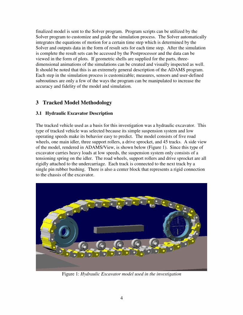
The tracked vehicle used as a basis for this investigation was a hydraulic excavator. This

type of tracked vehicle was selected because its simple suspension system and low

operating speeds make its behavior easy to predict. The model consists of five road

wheels, one main idler, three support rollers, a drive sprocket, and 45 tracks. A side view

of the model, rendered in ADAMS/View, is shown below (Figure 1). Since this type of

excavator carries heavy loads at low speeds, the suspension system only consists of a

tensioning spring on the idler. The road wheels, support rollers and drive sprocket are all

rigidly attached to the undercarriage. Each track is connected to the next track by a

single pin rubber bushing. There is also a center block that represents a rigid connection

to the chassis of the excavator.

Figure 1: Hydraulic Excavator model used in the investigation

5

3.2 Hydraulic Excavator Model

The physical model of a hydraulic excavator was implemented in ADAMS using the

following methods. Each individual track was connected to its two adjacent tracks by

means of a revolute joint about the center of each pin hole, with coulomb friction in the

joint to represent the behavior of a single pin rubber bushing. Contact forces between

each track solid and each contact body were created. Each track comes into contact with:

five road wheels, the idler, three support rollers, each of the three solids comprising the

drive sprocket, and the ground block. Therefore, there are 45*13 or 585 contact forces in

the model. Calculating contact forces is very computationally demanding; they create

very large reaction forces, which results in motion that requires very small time steps to

resolve accurately. Simulating the large number of contact forces present throughout the

simulation is the major bottleneck in tracked vehicle simulations. In the past, tracked

vehicle simulations have used a super-element to describe the behavior of the track

system because of the lack of computer power to represent each track and its

representative contact forces individually. This method has many drawbacks, including

the necessity of testing a physical model to get the data to convert the track system into a

super-element, and the inability to change the design of the track system once a super-

element has been created. Creating a super-element in place of the track system defeats

the purpose of virtual-prototyping and must be avoided if computer modeling and

simulation is to be used effectively in the design process of tracked vehicles.

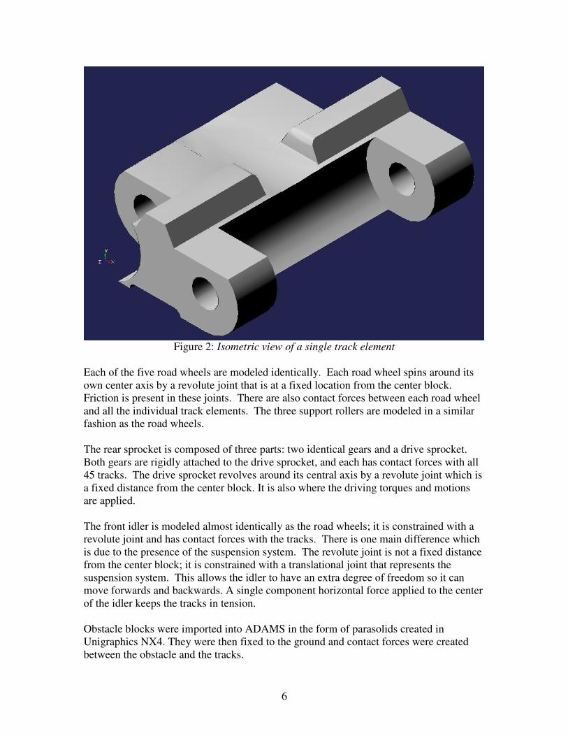
All of the track parts use the same geometry and therefore have the same parameters.

The material of the track is steel; using the density associated with steel and the volume

of an individual track, the calculated mass is approximately 498 kg. The overall width,

depth and length are: 625mm, 275mm and 900mm, respectively. Width, depth and

length correspond to the X, Y and Z directions, respectively, in Figure 2. It is apparent

from Figure 2 shown below that the modeled bushing pin is loaded under double shear.

The diameter of each hole is 100mm.

6

Figure 2: Isometric view of a single track element

Each of the five road wheels are modeled identically. Each road wheel spins around its

own center axis by a revolute joint that is at a fixed location from the center block.

Friction is present in these joints. There are also contact forces between each road wheel

and all the individual track elements. The three support rollers are modeled in a similar

fashion as the road wheels.

The rear sprocket is composed of three parts: two identical gears and a drive sprocket.

Both gears are rigidly attached to the drive sprocket, and each has contact forces with all

45 tracks. The drive sprocket revolves around its central axis by a revolute joint which is

a fixed distance from the center block. It is also where the driving torques and motions

are applied.

The front idler is modeled almost identically as the road wheels; it is constrained with a

revolute joint and has contact forces with the tracks. There is one main difference which

is due to the presence of the suspension system. The revolute joint is not a fixed distance

from the center block; it is constrained with a translational joint that represents the

suspension system. This allows the idler to have an extra degree of freedom so it can

move forwards and backwards. A single component horizontal force applied to the center

of the idler keeps the tracks in tension.

Obstacle blocks were imported into ADAMS in the form of parasolids created in

Unigraphics NX4. They were then fixed to the ground and contact forces were created

between the obstacle and the tracks.

7

4 Virtual Testing Conditions

In order to gain a better understanding of the mechanics involved in tracked vehicle

simulations, the model was tested under multiple conditions. The three independent

variables chosen to create different operating conditions were: the ground block, the

propulsion method, and the rate of the propulsion method. Eight trial simulations were

run to be able to judge the effect of the interactions between the independent variables.

Using both a flat running surface and one with an obstacle gave insight into how the

reaction forces affect performance on non-flat surfaces. This kind of testing is ideal for

any vehicle that is designed to operate in off-road conditions. The obstacle used in place

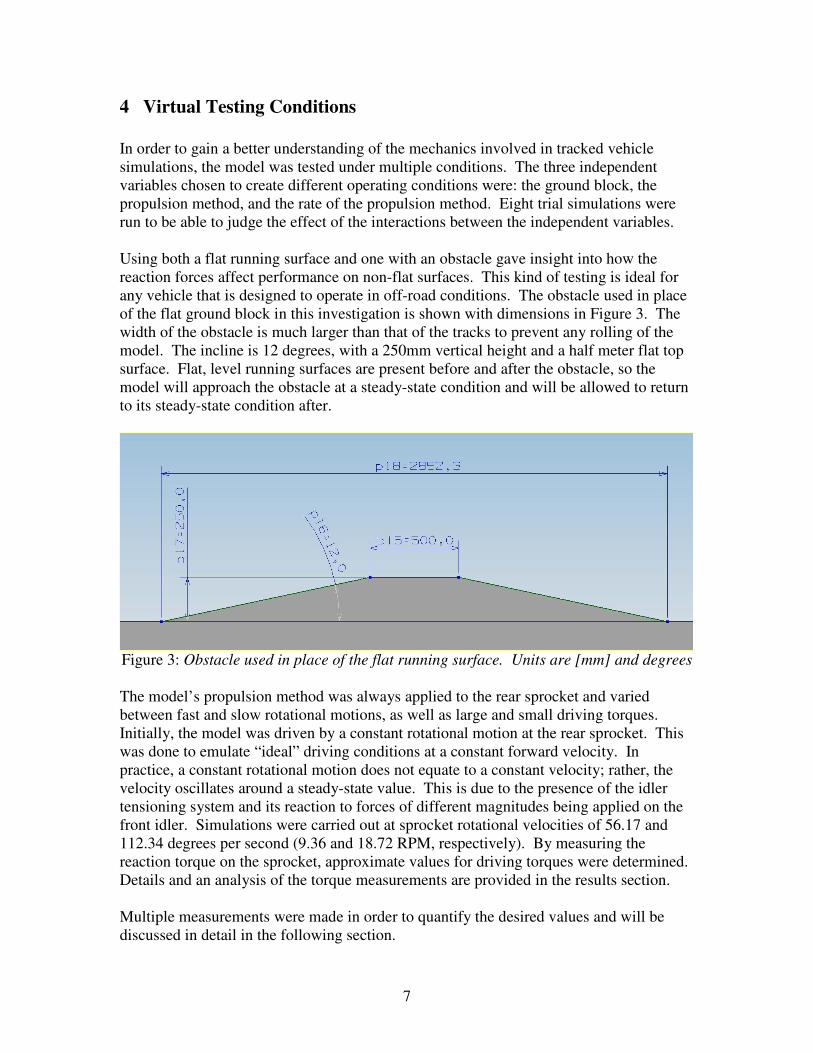
of the flat ground block in this investigation is shown with dimensions in Figure 3. The

width of the obstacle is much larger than that of the tracks to prevent any rolling of the

model. The incline is 12 degrees, with a 250mm vertical height and a half meter flat top

surface. Flat, level running surfaces are present before and after the obstacle, so the

model will approach the obstacle at a steady-state condition and will be allowed to return

to its steady-state condition after.

Figure 3: Obstacle used in place of the flat running surface. Units are [mm] and degrees

The model’s propulsion method was always applied to the rear sprocket and varied

between fast and slow rotational motions, as well as large and small driving torques.

Initially, the model was driven by a constant rotational motion at the rear sprocket. This

was done to emulate “ideal” driving conditions at a constant forward velocity. In

practice, a constant rotational motion does not equate to a constant velocity; rather, the

velocity oscillates around a steady-state value. This is due to the presence of the idler

tensioning system and its reaction to forces of different magnitudes being applied on the

front idler. Simulations were carried out at sprocket rotational velocities of 56.17 and

112.34 degrees per second (9.36 and 18.72 RPM, respectively). By measuring the

reaction torque on the sprocket, approximate values for driving torques were determined.

Details and an analysis of the torque measurements are provided in the results section.

Multiple measurements were made in order to quantify the desired values and will be

discussed in detail in the following section.

8

5 Results

As was stated previously, eight simulations were conducted with the tracked vehicle

model under different operating conditions. Measures were created to gauge different

aspects of the vehicle’s performance throughout the simulations. Some measures were

specific to certain independent variables, such as the angle of incline of the track as it

encounters an obstacle. Others were applicable to all the simulations; the force present in

the revolute joint between tracks is an example of this. Each measure will be described

and analyzed in detail in the subsequent sections.

5.1 Description of Measures

Before a torque could be applied as the driving method of the model, an appropriate

numerical value for the torque needed to be determined. For the simulation to succeed,

the torque needed to be large enough to overcome static friction; however, an excessively

large value would make the model move faster than it does in reality. The goal was to

apply a torque that would result in a comparable forward velocity as was attained when a

constant angular velocity was applied to the drive sprocket. This desired value was

obtained by measuring the torque on the rear sprocket’s revolute joint. It should be noted

that the torque varied substantially; between 0 and 7.43*105 N-m. This large variance

was investigated and appropriate values for the constant driving torque were determined.

The average values were obtained for the slow and fast motions and used for the trials

involving the model being driven by a torque.

The forward velocity of the model was of particular interest for two reasons. First, when

a constant driving torque is applied, the time it takes the model to reach its steady state

velocity marks the point in which the friction forces in the model have completely

transitioned from their static to dynamic values. The rate of this transition on flat ground

is examined. Second, it can show how substantially an impact with obstacles affects the

speed of the vehicle. The center marker of the central block was used to measure the

model’s velocity in the forward (negative x) direction.

When designing tracked vehicles that operate at high velocities, such as the M1A1

Abrams tank, the shearing stresses experienced by the bushings between the tracks

becomes very important. The strength and reliability of these components can become a

limiting factor as far as maximum vehicle speed is concerned. In order to determine the

shear stress in the bushings, a measurement of the magnitude of the force in the revolute

joint between track one and track two was made. This revolute joint was chosen because

it explores all the probable points of maximum stress. It begins the simulation

underneath one of the road wheels, is pulled around the sprocket, and moves some

distance across the top portion of the track. A picture of the joint described is shown in

Figure 4 below. The cross sectional area of the joint was then utilized to compute the

shear stress from the forces present in the joint. Values of the shear stress measurements

do not have any significance apart from their relative magnitude. In order to compute

shear stresses that correlate to actual values, an entire hydraulic excavator model or a

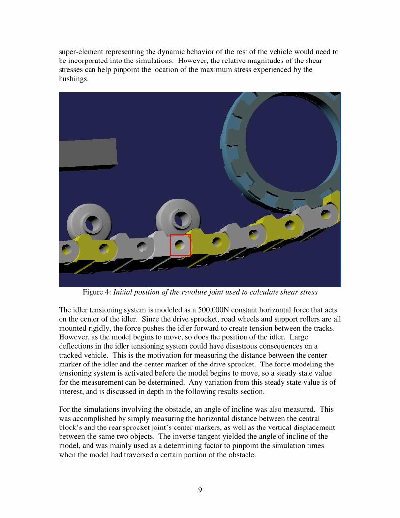
9

super-element representing the dynamic behavior of the rest of the vehicle would need to

be incorporated into the simulations. However, the relative magnitudes of the shear

stresses can help pinpoint the location of the maximum stress experienced by the

bushings.

Figure 4: Initial position of the revolute joint used to calculate shear stress

The idler tensioning system is modeled as a 500,000N constant horizontal force that acts

on the center of the idler. Since the drive sprocket, road wheels and support rollers are all

mounted rigidly, the force pushes the idler forward to create tension between the tracks.

However, as the model begins to move, so does the position of the idler. Large

deflections in the idler tensioning system could have disastrous consequences on a

tracked vehicle. This is the motivation for measuring the distance between the center

marker of the idler and the center marker of the drive sprocket. The force modeling the

tensioning system is activated before the model begins to move, so a steady state value

for the measurement can be determined. Any variation from this steady state value is of

interest, and is discussed in depth in the following results section.

For the simulations involving the obstacle, an angle of incline was also measured. This

was accomplished by simply measuring the horizontal distance between the central

block’s and the rear sprocket joint’s center markers, as well as the vertical displacement

between the same two objects. The inverse tangent yielded the angle of incline of the

model, and was mainly used as a determining factor to pinpoint the simulation times

when the model had traversed a certain portion of the obstacle.

10

5.2 Analysis of Measures

This section provides a detailed analysis of each of the measures described above. The

relative magnitudes of the measures rather than the values themselves is what will be

examined since this investigation only models the tracked propulsion system of a

hydraulic excavator, and not the entire vehicle. Nevertheless, an improved understanding

of the behavior of a simulated tracked vehicle can be achieved, which will help guide

future work and research in this field.

5.2.1 Driving Torque

As was stated in the previous section, an approximate value for the torque needed to be

determined before a constant torque could be applied as the propulsion method. Not only

did the torque need to be large enough to overcome static friction, but it would also need

to be sufficient to drive the model over an obstacle. Thus, it was decided that torque

measurements from the obstacle simulations where a constant sprocket angular velocity

driving method would be used. The average and RMS values of both the high and low

speed rotational motion simulations were computed in ADAMS/PostProcessor, for

1≤t≤10, where t is the simulation time in seconds. The values are calculated starting at

one second because the step functions describing the force on the idler tensioning system

and the rotational motion on the rear sprocket reach their final values after one second of

simulation time.

The average and root mean squared (RMS) values of the measured torque during the slow

rotational motion simulation were 7.83E7 and 9.56E7 N-mm, respectively. The average

and RMS values of the torque during the fast rotational motion simulation were 8.67E7

and 1.07E8 N-mm, respectively. Using these average and RMS values, it was decided to

use torques of 8E7 and 1E8 N-mm on the driving sprocket when the rotational motion

was deactivated and the driving torque was used as a propulsion method. Both torque

plots are shown below and the substantial variance in values as stated in section 5.1 can

be easily noticed.

11

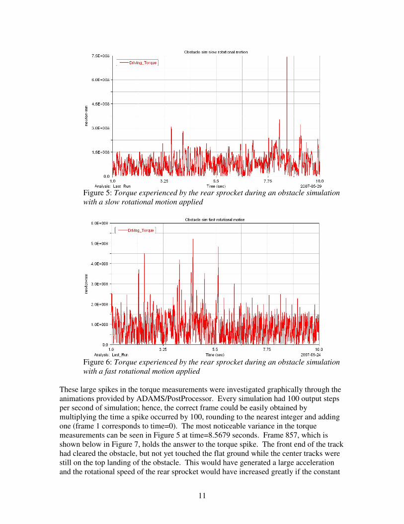
Figure 5: Torque experienced by the rear sprocket during an obstacle simulation

with a slow rotational motion applied

Figure 6: Torque experienced by the rear sprocket during an obstacle simulation

with a fast rotational motion applied

These large spikes in the torque measurements were investigated graphically through the

animations provided by ADAMS/PostProcessor. Every simulation had 100 output steps

per second of simulation; hence, the correct frame could be easily obtained by

multiplying the time a spike occurred by 100, rounding to the nearest integer and adding

one (frame 1 corresponds to time=0). The most noticeable variance in the torque

measurements can be seen in Figure 5 at time=8.5679 seconds. Frame 857, which is

shown below in Figure 7, holds the answer to the torque spike. The front end of the track

had cleared the obstacle, but not yet touched the flat ground while the center tracks were

still on the top landing of the obstacle. This would have generated a large acceleration

and the rotational speed of the rear sprocket would have increased greatly if the constant

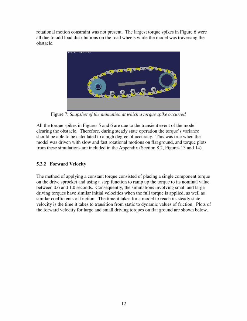
12

rotational motion constraint was not present. The largest torque spikes in Figure 6 were

all due to odd load distributions on the road wheels while the model was traversing the

obstacle.

Figure 7: Snapshot of the animation at which a torque spike occurred

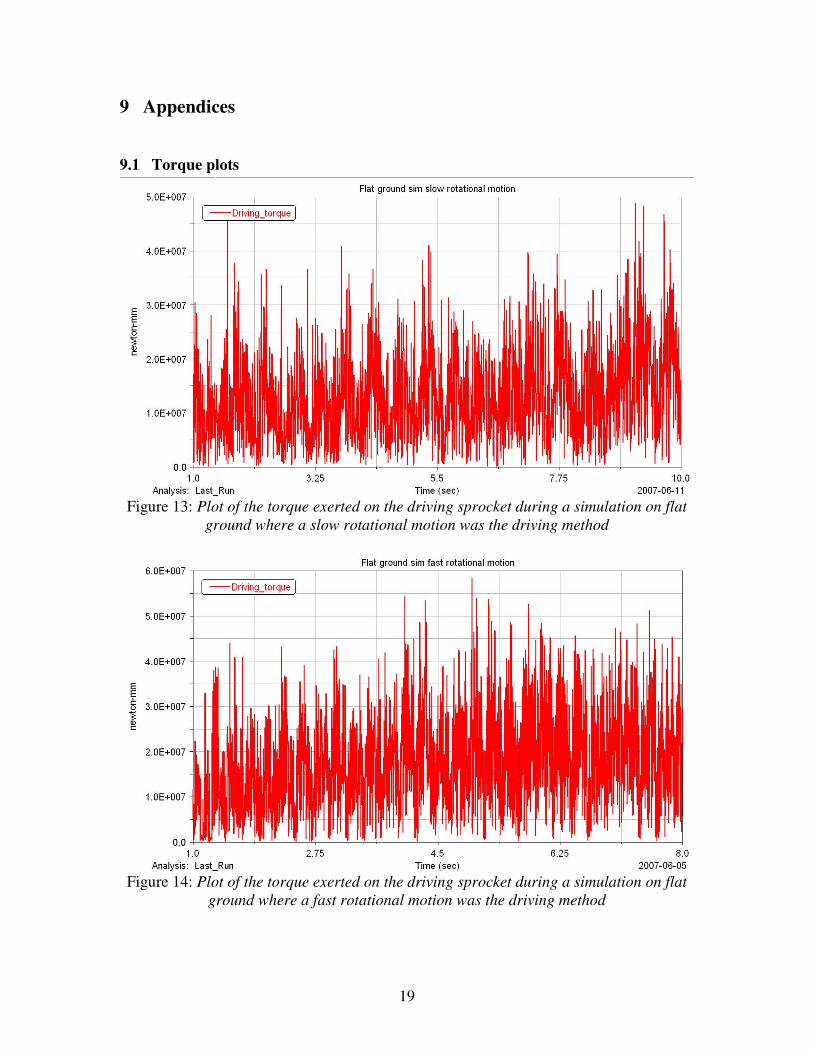
All the torque spikes in Figures 5 and 6 are due to the transient event of the model

clearing the obstacle. Therefore, during steady state operation the torque’s variance

should be able to be calculated to a high degree of accuracy. This was true when the

model was driven with slow and fast rotational motions on flat ground, and torque plots

from these simulations are included in the Appendix (Section 8.2, Figures 13 and 14).

5.2.2 Forward Velocity

The method of applying a constant torque consisted of placing a single component torque

on the drive sprocket and using a step function to ramp up the torque to its nominal value

between 0.6 and 1.0 seconds. Consequently, the simulations involving small and large

driving torques have similar initial velocities when the full torque is applied, as well as

similar coefficients of friction. The time it takes for a model to reach its steady state

velocity is the time it takes to transition from static to dynamic values of friction. Plots of

the forward velocity for large and small driving torques on flat ground are shown below.

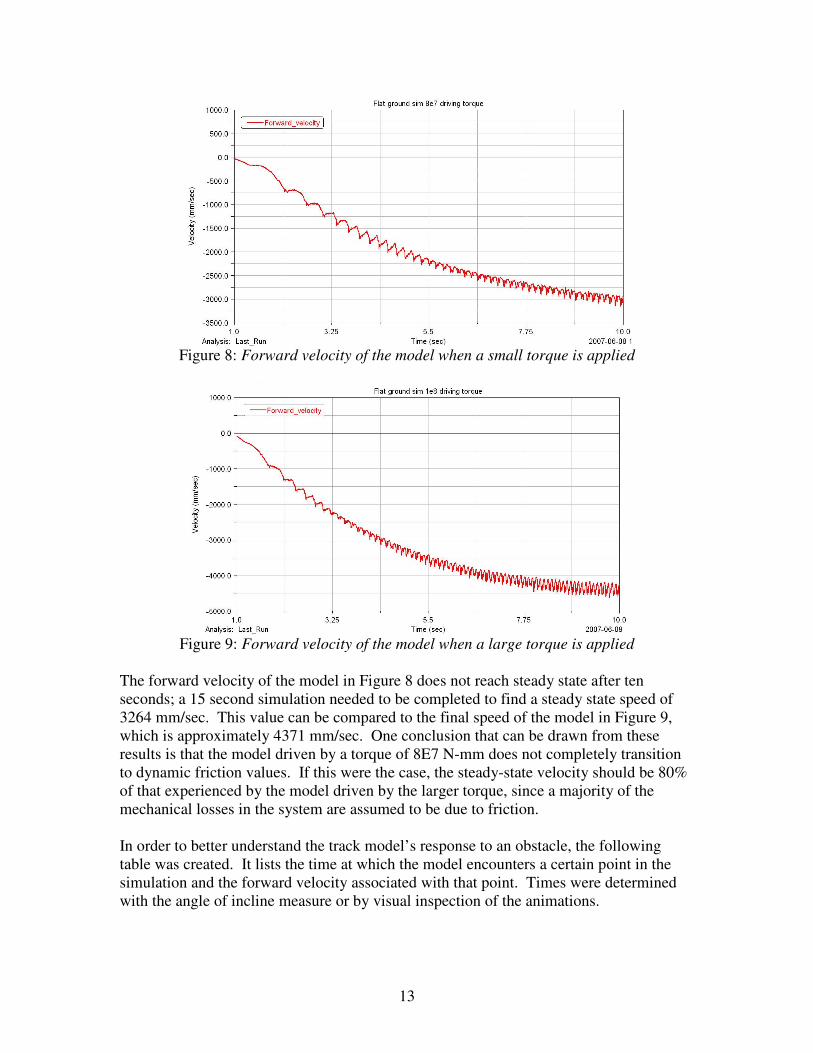
13

Figure 8: Forward velocity of the model when a small torque is applied

Figure 9: Forward velocity of the model when a large torque is applied

The forward velocity of the model in Figure 8 does not reach steady state after ten

seconds; a 15 second simulation needed to be completed to find a steady state speed of

3264 mm/sec. This value can be compared to the final speed of the model in Figure 9,

which is approximately 4371 mm/sec. One conclusion that can be drawn from these

results is that the model driven by a torque of 8E7 N-mm does not completely transition

to dynamic friction values. If this were the case, the steady-state velocity should be 80%

of that experienced by the model driven by the larger torque, since a majority of the

mechanical losses in the system are assumed to be due to friction.

In order to better understand the track model’s response to an obstacle, the following

table was created. It lists the time at which the model encounters a certain point in the

simulation and the forward velocity associated with that point. Times were determined

with the angle of incline measure or by visual inspection of the animations.

14

Table 1: Simulation time of certain events, and associated forward velocities

Model engages obstacle Model at peak of

obstacle

Model disengages

obstacle

Driving

Torque

[N-mm]

Simulation

time [s]

Velocity

[mm/sec]

Simulation

time[s]

Velocity

[mm/sec]

Simulation

time[s]

Velocity

[mm/sec]

8*107 3.67 1431 6.03 1434 7.68 2597

1*108 2.86 1842 4.47 2238 5.71 3510

This table shows that the smaller driving torque is just large enough for the model to

maintain its forward velocity when encountering the obstacle and can be proved with the

forward velocity plot for this simulation (Appendix 8.2). Once static friction is

overcome, the model has no problems traversing a small obstacle.

5.2.3 Modeled Bushing Shear Stress

Even though actual bushings were not used in this simulation, revolute joints with

corresponding frictional forces were used to approximate their behavior. Thus, the forces

being transferred through the revolute joints are the same forces that would be applied to

the bushings. The shear stresses resulting from these forces were analyzed for the flat

ground simulation when a small and large constant torque was applied. Using a bushing

diameter of approximately 100 mm, and knowing the loading case is double shear (See

Figure 2), the area used for shear stress calculations is 0.01571 m2. The following table

lists the simulation times at which the revolute joint is at a location where large shear

stresses are likely. Times were obtained graphically from the animations and are not

exact.

Table 2: Simulation time of certain positions of measured joint

Driving

Torque [N-

mm]

Encounters

road wheel [s]

Engages drive

sprocket [s]

Disengages drive

sprocket [s]

Encounters first

support roller [s]

8*107 2.01 3.39 4.85 5.49

1*108 1.62 2.63 3.77 4.24

Shearing stresses at the listed times can be calculated by dividing the force in the joint at

the given time by the cross sectional area calculated above.

Table 3: Calculated Shear Stress at Various Joint Positions

Driving

Torque [N-

mm]

Encounters road

wheel [MPa]

Engages drive

sprocket [MPa]

Disengages drive

sprocket [MPa]

Encounters first support

roller [MPa]

8*107 17.70 18.40 15.02 15.79

1*108 19.42 19.03 13.88 17.76

15

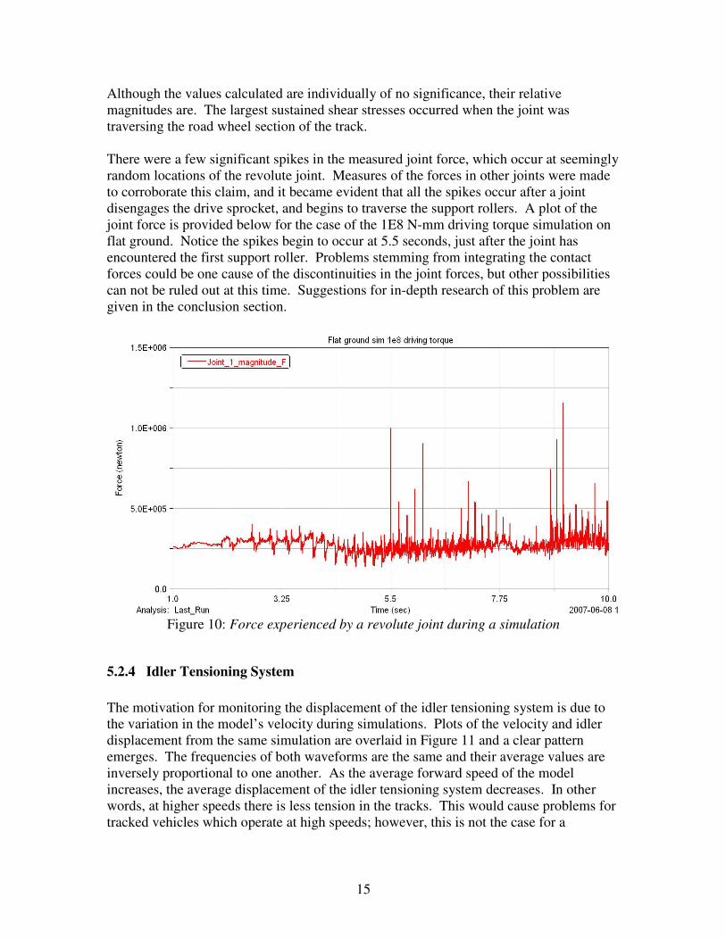
Although the values calculated are individually of no significance, their relative

magnitudes are. The largest sustained shear stresses occurred when the joint was

traversing the road wheel section of the track.

There were a few significant spikes in the measured joint force, which occur at seemingly

random locations of the revolute joint. Measures of the forces in other joints were made

to corroborate this claim, and it became evident that all the spikes occur after a joint

disengages the drive sprocket, and begins to traverse the support rollers. A plot of the

joint force is provided below for the case of the 1E8 N-mm driving torque simulation on

flat ground. Notice the spikes begin to occur at 5.5 seconds, just after the joint has

encountered the first support roller. Problems stemming from integrating the contact

forces could be one cause of the discontinuities in the joint forces, but other possibilities

can not be ruled out at this time. Suggestions for in-depth research of this problem are

given in the conclusion section.

Figure 10: Force experienced by a revolute joint during a simulation

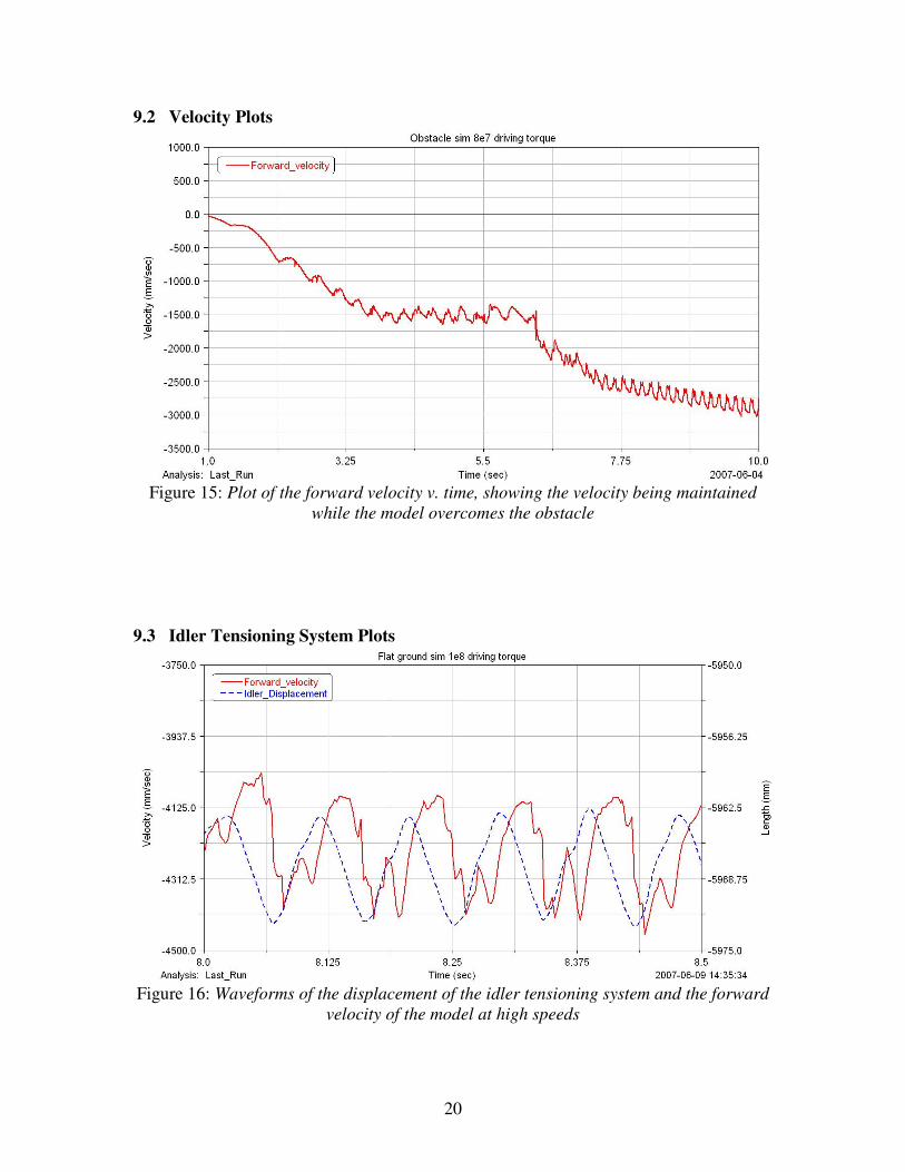
5.2.4 Idler Tensioning System

The motivation for monitoring the displacement of the idler tensioning system is due to

the variation in the model’s velocity during simulations. Plots of the velocity and idler

displacement from the same simulation are overlaid in Figure 11 and a clear pattern

emerges. The frequencies of both waveforms are the same and their average values are

inversely proportional to one another. As the average forward speed of the model

increases, the average displacement of the idler tensioning system decreases. In other

words, at higher speeds there is less tension in the tracks. This would cause problems for

tracked vehicles which operate at high speeds; however, this is not the case for a

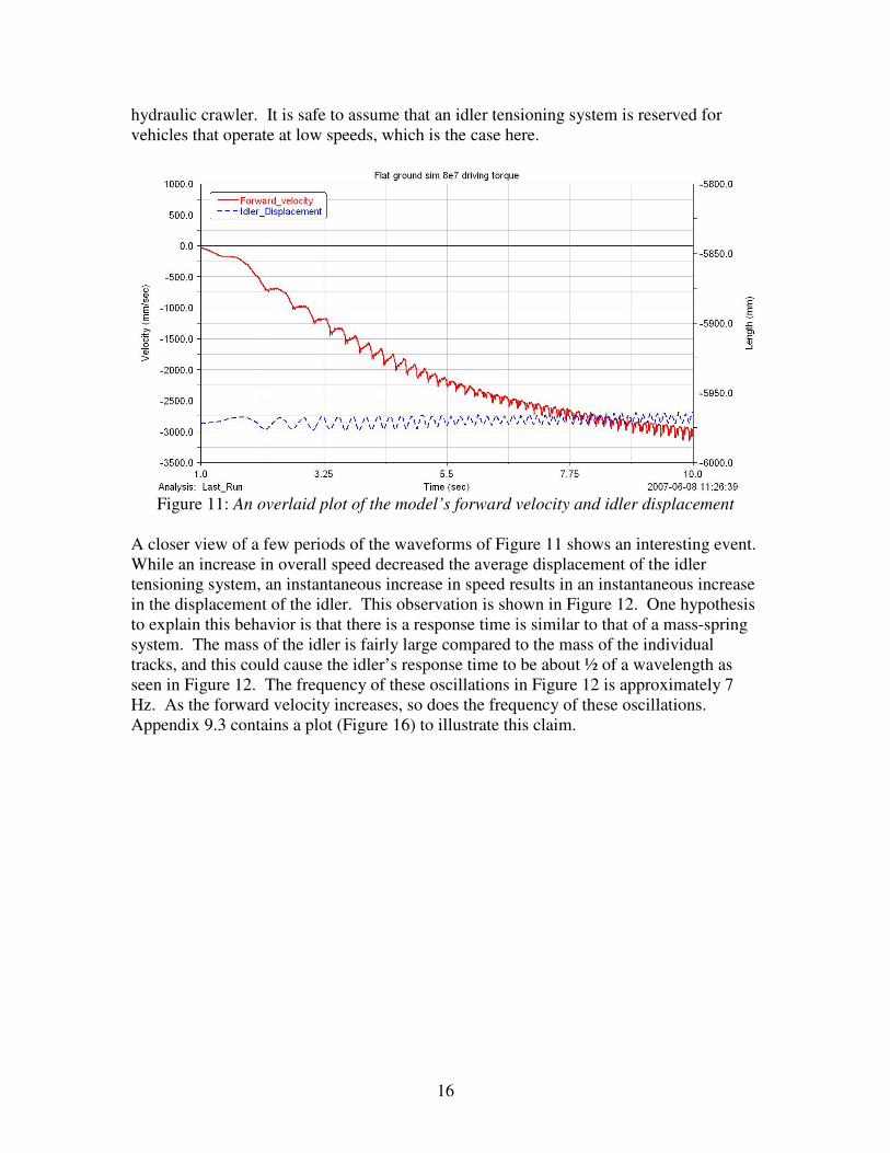
16

hydraulic crawler. It is safe to assume that an idler tensioning system is reserved for

vehicles that operate at low speeds, which is the case here.

Figure 11: An overlaid plot of the model’s forward velocity and idler displacement

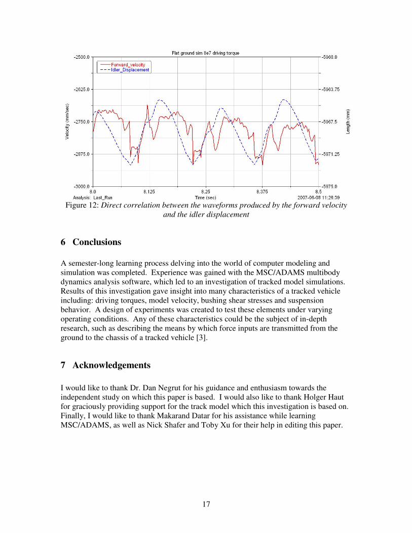
A closer view of a few periods of the waveforms of Figure 11 shows an interesting event.

While an increase in overall speed decreased the average displacement of the idler

tensioning system, an instantaneous increase in speed results in an instantaneous increase

in the displacement of the idler. This observation is shown in Figure 12. One hypothesis

to explain this behavior is that there is a response time is similar to that of a mass-spring

system. The mass of the idler is fairly large compared to the mass of the individual

tracks, and this could cause the idler’s response time to be about ½ of a wavelength as

seen in Figure 12. The frequency of these oscillations in Figure 12 is approximately 7

Hz. As the forward velocity increases, so does the frequency of these oscillations.

Appendix 9.3 contains a plot (Figure 16) to illustrate this claim.

17

Figure 12: Direct correlation between the waveforms produced by the forward velocity

and the idler displacement

6 Conclusions

A semester-long learning process delving into the world of computer modeling and

simulation was completed. Experience was gained with the MSC/ADAMS multibody

dynamics analysis software, which led to an investigation of tracked model simulations.

Results of this investigation gave insight into many characteristics of a tracked vehicle

including: driving torques, model velocity, bushing shear stresses and suspension

behavior. A design of experiments was created to test these elements under varying

operating conditions. Any of these characteristics could be the subject of in-depth

research, such as describing the means by which force inputs are transmitted from the

ground to the chassis of a tracked vehicle [3].

7 Acknowledgements

I would like to thank Dr. Dan Negrut for his guidance and enthusiasm towards the

independent study on which this paper is based. I would also like to thank Holger Haut

for graciously providing support for the track model which this investigation is based on.

Finally, I would like to thank Makarand Datar for his assistance while learning

MSC/ADAMS, as well as Nick Shafer and Toby Xu for their help in editing this paper.

18

8 References

[1] Holger Haut, http://www.multibodysimulation.com

[2] Simulation Based Engineering Laboratory, University of Wisconsin-Madison,

http://sbel.wisc.edu/

[3] Allen, P., “Models for the dynamic simulation of tank track components.” PhD

Thesis, Cranfield University, 2006.

[4] Letherwood, D., Gunter, D. D., “Ground vehicle modeling and simulation of

military vehicles using high performance computing.” Parallel Computing 27

(2001) 109-140.

[5] Rubinstein, D., Hitron, R., “A detailed multi-body model for dynamic simulation

of off-road tracked vehicles.” Journal of Terramechanics 41 (2004) 163-173.

[6] Gunter, D., et al. “Using 3D multi-body simulation to evaluate future truck

technologies.” SAE paper 2005-01-0934.

[7] Gorsich, D., et al. “Terrain roughness standards for mobility and ultra-reliability

prediction.” SAE paper 2003-01-0218.

[8] MSC.ADAMS 2005, “Basic ADAMS/Solver training guide.”

19

9 Appendices

9.1 Torque plots

Figure 13: Plot of the torque exerted on the driving sprocket during a simulation on flat

ground where a slow rotational motion was the driving method

Figure 14: Plot of the torque exerted on the driving sprocket during a simulation on flat

ground where a fast rotational motion was the driving method

20

9.2 Velocity Plots

Figure 15: Plot of the forward velocity v. time, showing the velocity being maintained

while the model overcomes the obstacle

9.3 Idler Tensioning System Plots

Figure 16: Waveforms of the displacement of the idler tensioning system and the forward

velocity of the model at high speeds