Embed Size (px)
Citation preview

High Efficiency Electric Generator for Chain-less
Bicycleby
Fernando Alvarez Gonzalez
Submitted to the Department of Electrical Engineering, Electronics,Computers and Systems
in partial fulfillment of the requirements for the degree of
Electrical Energy Conversion and Power Systems
at the
UNIVERSIDAD DE OVIEDO
July 2014
c© Universidad de Oviedo 2014. All rights reserved.
Author . . . . . . . . . . . . . . . . . . . . . . . . . . . . . . . . . . . . . . . . . . . . . . . . . . . . . . . . . . . . . .
Certified by. . . . . . . . . . . . . . . . . . . . . . . . . . . . . . . . . . . . . . . . . . . . . . . . . . . . . . . . . .Pablo Garcıa Fernandez
Associate ProfessorThesis Supervisor
Certified by. . . . . . . . . . . . . . . . . . . . . . . . . . . . . . . . . . . . . . . . . . . . . . . . . . . . . . . . . .Chris Gerada
ProfessorThesis Supervisor

2

High Efficiency Electric Generator for Chain-less Bicycle
by
Fernando Alvarez Gonzalez
Submitted to the Department of Electrical Engineering, Electronics, Computers andSystems
on July 25, 2014, in partial fulfillment of therequirements for the degree of
Electrical Energy Conversion and Power Systems
Abstract
In this thesis, an electric generator for a chain-less bicycle was designed, optimizedand studied in detail. Following a design methodology and employing powerful soft-ware tools, the different characteristics were tested through simulation and taken tothe limit of its efficiency. Optimization curves were developed for the main parame-ters and simulation results were provided and studied both analytically and throughsoftware analysis. A final satisfactory model was provided and will be manufacturedin a near future.
The entire project has been developed within the PEMC (Power Electronics andMachine Control) group at the University of Nottingham.
Thesis Supervisor: Pablo Garcıa FernandezTitle: Associate Professor
Thesis Supervisor: Chris GeradaTitle: Professor
3

4

Acknowledgments
This project has been entirely developed within the PEMC (Power Electronics and
Machine Control) group at the University of Nottingham and it couldn’t have been
possible without the collaboration of this institution and its members, especially
Professor Chris Gerada and research fellow Puvan Arumugam.
Special thanks to all PEMC group members who welcomed me without hesitation
and managed to make me feel at home.
5

6
Contents
Glossary 14
1 Introduction 17
1.1 Objectives . . . . . . . . . . . . . . . . . . . . . . . . . . . . . . . . . 18
1.2 State of the art . . . . . . . . . . . . . . . . . . . . . . . . . . . . . . 18
1.2.1 Generators for electric bicycles . . . . . . . . . . . . . . . . . . 19
1.2.2 Chain-less electric bicycles . . . . . . . . . . . . . . . . . . . . 20
2 Generator design 21
2.1 Constraints . . . . . . . . . . . . . . . . . . . . . . . . . . . . . . . . 21
2.1.1 Size . . . . . . . . . . . . . . . . . . . . . . . . . . . . . . . . 22
2.1.2 Torque . . . . . . . . . . . . . . . . . . . . . . . . . . . . . . . 22
2.1.3 Voltage . . . . . . . . . . . . . . . . . . . . . . . . . . . . . . 22
2.1.4 Others . . . . . . . . . . . . . . . . . . . . . . . . . . . . . . . 22
2.2 Initial model search . . . . . . . . . . . . . . . . . . . . . . . . . . . . 23
2.2.1 Topologies comparison . . . . . . . . . . . . . . . . . . . . . . 23
2.2.2 Configuration comparison . . . . . . . . . . . . . . . . . . . . 24
2.2.3 Initial values . . . . . . . . . . . . . . . . . . . . . . . . . . . 26
2.3 Design methodology . . . . . . . . . . . . . . . . . . . . . . . . . . . 29
2.3.1 Software tools . . . . . . . . . . . . . . . . . . . . . . . . . . . 29
3 Model optimization 33
3.1 Major parameter changes . . . . . . . . . . . . . . . . . . . . . . . . . 33
7

3.1.1 Number of turns and supply current . . . . . . . . . . . . . . 33
3.1.2 Magnet thickness . . . . . . . . . . . . . . . . . . . . . . . . . 34
3.1.3 Magnet angle . . . . . . . . . . . . . . . . . . . . . . . . . . . 36
3.1.4 Rotor diameter . . . . . . . . . . . . . . . . . . . . . . . . . . 37
3.1.5 Tooth Width Ratio . . . . . . . . . . . . . . . . . . . . . . . . 37
3.2 Parametric changes . . . . . . . . . . . . . . . . . . . . . . . . . . . . 39
3.2.1 Slot opening . . . . . . . . . . . . . . . . . . . . . . . . . . . . 40
3.2.2 Slot wedge angle . . . . . . . . . . . . . . . . . . . . . . . . . 41
3.2.3 Tooth tip height . . . . . . . . . . . . . . . . . . . . . . . . . 44
4 Characteristics study 47
4.1 Air-gap flux density . . . . . . . . . . . . . . . . . . . . . . . . . . . . 47
4.2 Phase flux linkage . . . . . . . . . . . . . . . . . . . . . . . . . . . . . 49
4.3 Back EMF . . . . . . . . . . . . . . . . . . . . . . . . . . . . . . . . . 51
4.4 Torque . . . . . . . . . . . . . . . . . . . . . . . . . . . . . . . . . . . 52
4.4.1 Average torque . . . . . . . . . . . . . . . . . . . . . . . . . . 52
4.4.2 Cogging torque . . . . . . . . . . . . . . . . . . . . . . . . . . 53
4.4.3 Torque ripple . . . . . . . . . . . . . . . . . . . . . . . . . . . 54
4.5 Current density . . . . . . . . . . . . . . . . . . . . . . . . . . . . . . 55
4.6 Copper Losses . . . . . . . . . . . . . . . . . . . . . . . . . . . . . . . 57
4.7 Iron Losses . . . . . . . . . . . . . . . . . . . . . . . . . . . . . . . . 58
4.7.1 Hysteresis . . . . . . . . . . . . . . . . . . . . . . . . . . . . . 59
4.7.2 Eddy Current . . . . . . . . . . . . . . . . . . . . . . . . . . . 59
4.8 Demagnetization and variation with temperature . . . . . . . . . . . 61
4.8.1 Remanent flux density . . . . . . . . . . . . . . . . . . . . . . 61
4.8.2 Coercivity . . . . . . . . . . . . . . . . . . . . . . . . . . . . . 62
4.9 Radial forces . . . . . . . . . . . . . . . . . . . . . . . . . . . . . . . . 62
5 Conclusion 65
5.1 Future Work . . . . . . . . . . . . . . . . . . . . . . . . . . . . . . . . 65
8

Bibliography 67
9

10
List of Figures
1-1 Bicycle Concept Example . . . . . . . . . . . . . . . . . . . . . . . . 18
2-1 Inset Permanent Magnet Generator Example . . . . . . . . . . . . . . 24
2-2 Surface Permanent Magnet Generator Example . . . . . . . . . . . . 25
2-3 MagNet Software Winding Phase A . . . . . . . . . . . . . . . . . . . 28
2-4 Motor Solve Software Tool Example . . . . . . . . . . . . . . . . . . . 30
2-5 Motor Solve Software Tool Results . . . . . . . . . . . . . . . . . . . 31
2-6 MagNet Software Tool Flux Results . . . . . . . . . . . . . . . . . . . 32
2-7 MagNet Software Finite Element Mesh . . . . . . . . . . . . . . . . . 32
3-1 Magnet Thickness versus Efficiency . . . . . . . . . . . . . . . . . . . 35
3-2 Magnet Thickness versus Torque . . . . . . . . . . . . . . . . . . . . . 36
3-3 Magnet Thickness versus Voltage . . . . . . . . . . . . . . . . . . . . 36
3-4 Tooth Width Ratio equal to 0.5 . . . . . . . . . . . . . . . . . . . . . 38
3-5 Tooth Width Ratio equal to 0.7 . . . . . . . . . . . . . . . . . . . . . 38
3-6 Tooth Width Ratio versus Efficiency . . . . . . . . . . . . . . . . . . 39
3-7 Tooth Width Ratio versus Torque . . . . . . . . . . . . . . . . . . . . 39
3-8 Slot Opening versus Efficiency . . . . . . . . . . . . . . . . . . . . . . 40
3-9 Slot Opening versus Torque . . . . . . . . . . . . . . . . . . . . . . . 41
3-10 Slot Opening equal to 0.5 . . . . . . . . . . . . . . . . . . . . . . . . 41
3-11 Slot Opening equal to 5 . . . . . . . . . . . . . . . . . . . . . . . . . 42
3-12 Slot Opening versus Voltage . . . . . . . . . . . . . . . . . . . . . . . 42
3-13 Slot wedge angle equal to 5 . . . . . . . . . . . . . . . . . . . . . . . 43
3-14 Slot wedge angle equal to 35 . . . . . . . . . . . . . . . . . . . . . . . 43
11

3-15 Slot Wedge Angle versus Efficiency . . . . . . . . . . . . . . . . . . . 44
3-16 Slot Wedge Angle versus Torque . . . . . . . . . . . . . . . . . . . . . 44
4-1 Flux Density . . . . . . . . . . . . . . . . . . . . . . . . . . . . . . . 48
4-2 Flux Density Detailed . . . . . . . . . . . . . . . . . . . . . . . . . . 48
4-3 Flux Linkage due to Permanent Magnets . . . . . . . . . . . . . . . . 50
4-4 Total Flux Linkage . . . . . . . . . . . . . . . . . . . . . . . . . . . . 50
4-5 Back Electromotive Force . . . . . . . . . . . . . . . . . . . . . . . . 52
4-6 Torque . . . . . . . . . . . . . . . . . . . . . . . . . . . . . . . . . . . 53
4-7 Cogging Torque . . . . . . . . . . . . . . . . . . . . . . . . . . . . . . 54
4-8 Current Density . . . . . . . . . . . . . . . . . . . . . . . . . . . . . . 56
4-9 Half Slot Copper Losses . . . . . . . . . . . . . . . . . . . . . . . . . 57
4-10 Magnet Eddy Current Losses . . . . . . . . . . . . . . . . . . . . . . 60
12

List of Tables
2.1 Windings Table . . . . . . . . . . . . . . . . . . . . . . . . . . . . . . 27
5.1 Final Model Characteristics . . . . . . . . . . . . . . . . . . . . . . . 66
5.2 Final Model Results . . . . . . . . . . . . . . . . . . . . . . . . . . . 66
13

14

Glossary
SPM Surface Permanent Magnet
IPM Interior Permanent Magnet
B Flux Density
Br Remanent Flux Density
λ Flux Linkage
Hc Coercivity
µr Magnet Relative Permeability
Lg Air-gap Length (also g)
Lm Magnet Length or Thickness
φ Flux
A Electrical Loading
J Current Density
f Frequency
Lstk Stack or Axial Length
Nph Number of Turns per Phase
m Number of Phases
p Number of Pole Pairs
Pa Air-gap Permeance
Psl Slot Leakage Permeance
Irms Effective Value of Current Supply
Aslot Slot Area
Fslot Slot Fill Factor (also Kfill)
ρcu Electrical Resistivity of Copper
15

16
Chapter 1
Introduction
Since the invention of electric bicycle in the 1890’s the vast majority of progress have
due to the evolution of existing batteries, electronics and electric motors technology.
Very little has been innovated with regard to the concept of electric bicycle.
The market for electric bicycles is clearly on the rise both in the European Union
and beyond its borders. It is a novel alternative that promotes the protection of the
environment, the reduction of the carbon footprint, allows riding the bicycle with less
effort, making an intelligent management of electrical energy and enabling innovation
on their use as a mobile power source. Undoubtedly the evolution of the electric
bicycle will continue to create opportunities for development and business.
As it will be extensively presented later in the “state of the art” section, nowa-
days a great number of electric bicycles are based on the use of batteries to store a
limited amount of energy and then either assist a conventional mechanical connection
pedaling system or propel the bike for a limited time and distance.
The concept raised here radically changes the way an electric bike is understood.
In this system, the mechanical connection is eliminated as seen in figure 1-1 because
it has been taken to the limit of its cost-effective efficiency.
Instead, the connection is fully electrically made, the energy obtained from a
high-efficiency generator, manage by a power converter and used to power an electric
motor that will be the sole mean of propulsion for the bicycle for an unlimited time
or distance, as long as the user keeps pedaling. It is then, a pure electric bicycle.
17

Figure 1-1: Bicycle Concept Example
Through this thesis, the subject of study has been the high-efficiency generator
which for obvious reasons accounts for one of the crucial aspects of the system, being
the source for all power. The generator type chosen is a permanent magnet one in
order to reduce maintenance to the minimum as it avoids the frequent exchange of
brushes. Reducing maintenance is another of the crucial aspects which empowers
the realization of this project as mechanical transmissions require often a revision or
exchange of its pieces.
1.1 Objectives
The objectives of this project are to design a high-efficiency generator that fits the
constraints specified in chapter two, to develop and follow a design methodology which
allows optimizing the final model and to provide a detailed study of its characteristics.
1.2 State of the art
Although the concept of electric bicycle is not new, nowadays the vast majority of
bicycles of this type consist on bulky systems based on the use of batteries. This is in
fact nothing but a conventional bicycle with pedal assistance employing batteries and
usually a low power electric motor. This vehicles are commonly known as Pedelec.
18

The problem with most current bicycles is that they are transformations of con-
ventional ones with the addition of some electric systems, which is usually known
as hybrid-electric bicycles. Examples of this are well known manufacturers on the
field such as “LaFree”, “Panasonic” or the disappeared “Tidalforce”. The proposed
system is a full electrical design.
Regarding the legal status of electric bicycles, the European Union directive
2002/24/EC exempts vehicles with the following definition from type approval: “Cy-
cles with pedal assistance which are equipped with an auxiliary electric motor having
a maximum continuous rated power of 0.25 kW, of which the output is progressively
reduced and finally cut off as the vehicle reaches a speed of 25 km/h (16 mph) or if
the cyclist stops pedaling.” Based on this definition it is possible to affirm that the
proposed system is exempt as the lack of batteries will cause it to stop moving if the
cyclist stops pedaling.
Previously, some electric bicycle manufacturers were presented, some others are
displayed below:
• AVE Bikes
• Beixo
• BH E-Motion
• BIOBIKE Motoriza-
ciones
• Coluer
• Goes
• Grace Bikes
• Haibike
• Hercules
• Kettler
• Lapıerre
• Legend e-bikes
• Moustache Bikes
• Pedego
• Quipplan
• Wisper
• Yamimoto
• Urban Biker
1.2.1 Generators for electric bicycles
Due to the above specified legal issues most commercial electric bicycles nowadays
present brushless motors of 250W but it is not unusual to find power ratings between
120W like “Flebi’s Original” and 500W like most heavy or high speed electric bicycles
19

such as “A2B’s Shima”. One of the most seen companies involved in the electric
bicycle motors market is “Bosch”. Its machines are present in several designs from
different manufacturers. These bicycles usually employ Lithium-ion batteriesin the
range from 24-36V and 8-10Ah.
1.2.2 Chain-less electric bicycles
Nowadays one of the only known commercial electric chain-less bicycle is “Mando’s
Footloose” which, although has this revolutionary feature of having no chain, does
not get rid of the batteries and has a limited 20-mile operation range. This leaves
space in an unexplored market where it is intended to introduce the system under
study.
20

Chapter 2
Generator design
This section presents the first steps taken in the process of designing a generator. The
different constraints, topologies and model comparison methodology are introduced
in this chapter.
2.1 Constraints
Regarding design constraints, there are mainly three characteristics that were con-
sidered as crucial for the correct operation of the machine: Size, torque and voltage.
Each of them is presented independently below.
These constraints are a result of previous works regarding a whole electric bicycle
focused on mechanical design and power electronics. Size is crucial as it was a result
of the mechanical design, in case the outer size differs from the constraints, it would
not fit within the frame. Torque is another of the crucial aspects given that it is used
to obtain the total output power extracted from the generator and thus present on
the whole system, and finally voltage is important due to the power converter stage
which requests a certain value and also to avoid as much as possible having to boost
up it.
21
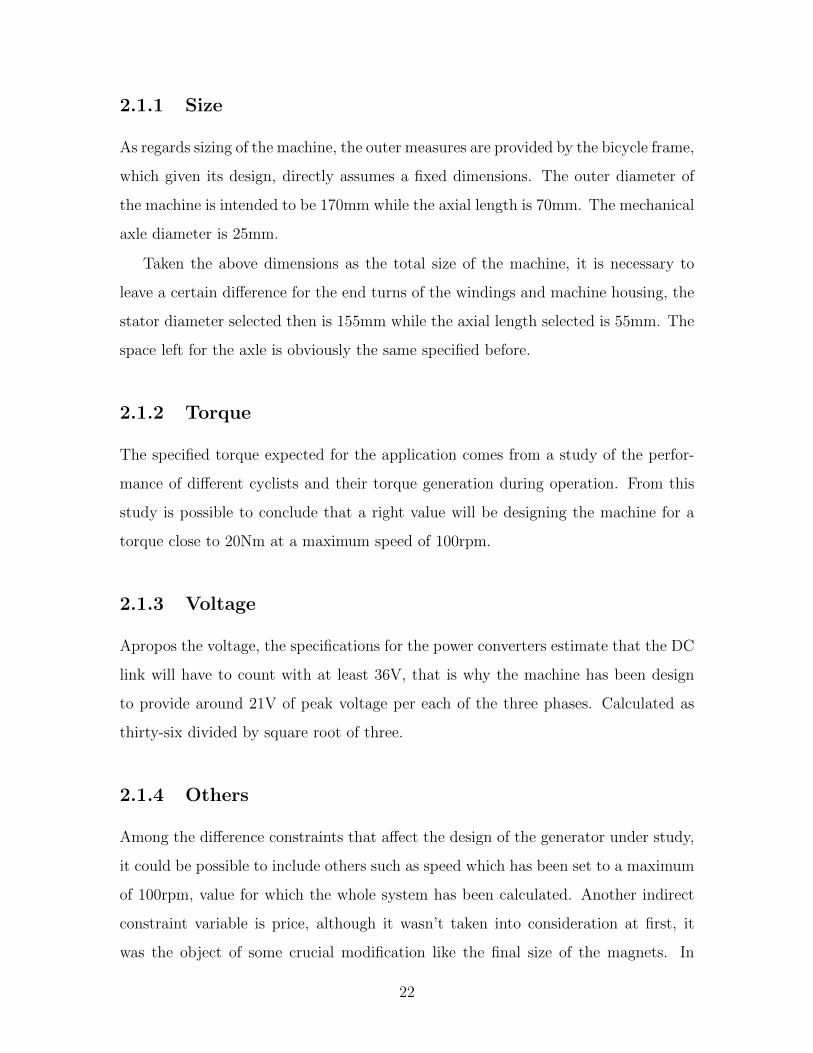
2.1.1 Size
As regards sizing of the machine, the outer measures are provided by the bicycle frame,
which given its design, directly assumes a fixed dimensions. The outer diameter of
the machine is intended to be 170mm while the axial length is 70mm. The mechanical
axle diameter is 25mm.
Taken the above dimensions as the total size of the machine, it is necessary to
leave a certain difference for the end turns of the windings and machine housing, the
stator diameter selected then is 155mm while the axial length selected is 55mm. The
space left for the axle is obviously the same specified before.
2.1.2 Torque
The specified torque expected for the application comes from a study of the perfor-
mance of different cyclists and their torque generation during operation. From this
study is possible to conclude that a right value will be designing the machine for a
torque close to 20Nm at a maximum speed of 100rpm.
2.1.3 Voltage
Apropos the voltage, the specifications for the power converters estimate that the DC
link will have to count with at least 36V, that is why the machine has been design
to provide around 21V of peak voltage per each of the three phases. Calculated as
thirty-six divided by square root of three.
2.1.4 Others
Among the difference constraints that affect the design of the generator under study,
it could be possible to include others such as speed which has been set to a maximum
of 100rpm, value for which the whole system has been calculated. Another indirect
constraint variable is price, although it wasn’t taken into consideration at first, it
was the object of some crucial modification like the final size of the magnets. In
22

this sense, the machine has been designed paying attention to cost-effective aspects.
Finally but not of lesser importance, avoiding saturation has played a relevant role
when undertaking upgrades for the final model. The variables that help against the
occurrence of saturation have been commented on chapter three.
2.2 Initial model search
In order to obtain a valid design model, the first step consists on providing an initial
case which, fulfilling constraints, serves as starting point for the design process. For
this purpose, different software tools, presented in detailed through design method-
ology’s section, have been employed in order to compare between several topologies
or configuration and choose.
2.2.1 Topologies comparison
While the initial thought was to design directly a surface mounted permanent mag-
net(SPM) generator, once started the process of selecting an initial model, it was seen
as useful to establish a shallow comparison with a topology of magnets located inside
the rotor, more specifically an inset permanent magnet generator.
Inset machines weren’t studied in detail as the main objective was to compare
certain features. It is possible to conclude that although this type of machine require
less number of turns allowing saving material they are better configured for higher
speeds than that of the application declared on the last section of constraints.
An example of possible configuration for this type of machine is presented in figure
2-1, which presents an inset 24/20 slot/pole configuration.
If compared to a surface permanent magnet generator, it is possible to notice also
that the complexity of the first one is greater which may come as another reason for
not selecting it. Also with the data obtained from simulation it would be possible to
affirm that at the current speed of operation, the efficiency for the surface machine
will be bigger. In order to visually allow that comparison declared previously, in
figure 2-2 it is possible to see the aspect that the final chosen model (also a 24/20
23

Figure 2-1: Inset Permanent Magnet Generator Example
slot/pole combination) presents.
2.2.2 Configuration comparison
By configuration, the referred design variable is the number of slots and poles, usu-
ally known as slot/pole combination. The number of slots and poles has a crucial
importance in a motor or generator. It is well known that for low speed applica-
tions the number of slots and poles tends to increase as it may be seen on the bigger
type of wind turbines been installed offshore in recent years. One reason for this is
the possibility of generating a more constant supply of torque and thus power while
maintaining low speed values. For high speed systems it is not necessary to include
a huge number of slots and poles as the interruptibility will be compensated by the
rapid rotation.
Initial models at the beginning of this project development presented a configu-
24

Figure 2-2: Surface Permanent Magnet Generator Example
ration of 12/10 slot/pole combination, as this is a very well tested and very usual
configuration which has been proven to work over the years. For many cases the
obtained models were proven to present a very good behavior, satisfying design con-
straints and proving successful when looking at its results. In fact, this configuration
could be satisfactory for the case under study as well. The reason why it wasn’t cho-
sen at the end is because as the maximum speed is 100rpm, truly, operation speed will
tend to be lower, in which case a machine with a higher number of slots and poles will
remain valid while the behavior of this one will, at some point, start decaying much
faster. In other terms there wouldn’t be much difference as well, for instance for price
as the size and the amount of conducting material would be necessarily maintained.
Apart from 12/10 and 24/20, which was presented on previous section, another
extremely similar configuration was compared, 24 slots and 22 poles. The reason
for comparing these three is not arbitrary as they all present good characteristics
for low speed as good winding factor and good pull-out torque [1]. Also the three
are diametrically symmetric which contrary to non-symmetric machines, increases
25

bearing life and reduces acoustic noise and vibration. Finally, 24/20 was chosen
over 24/22 for being considered as a slightly safer machine in terms of control and
recommended by advice of one of the project supervisors. In fact there is controversy
about which machine presents better characteristics.
Finally it is important to point out that at a very early stage of this project, a
vast number of slot/pole configurations were rejected for having variables far worse
than the one presented above. Among them there were the following:
• 12 slots / 14 poles
• 15 slots / 10 poles
• 15 slots / 14 poles
• 18 slots / 10 poles
• 24 slots / 28 poles
• 30 slots / 28 poles
2.2.3 Initial values
Initial values for most characteristics were obtained in most cases employing one of
the software tools which will be presented in following sections and then compared
to the values obtained through expressions in order to test its validity.
For instance, although it is possible to obtain the number of turns through various
expressions, it is much faster to provide an estimated value, simulate the system and
from there calculate in what measure will the obtained torque or voltage seem reduce
in relation with that value.
Once the results are approximated, it is easy to provide initial design variables
such as the current supply been given that in order to maintain the torque constant,
the result of multiplying number of turns and supply current must be maintained. In
this way, once the torque is at a valid point, lets say 20 newton-meter, the number of
turns and supply current can be modified to reduce losses, increase voltage or others
by for instance reducing that current and increasing the number of turns.
In this way, giving general initial values like a number of turns equal to 44, a supply
current equal to 10 amperes, a magnet thickness or height equal to 6 millimeters
it is possible to rapidly obtain and initial model which would, following a design
26

methodology, allow a further optimization with the consequent obtainment of a final
satisfactory model.
Windings
Winding type chosen is a two layer side-by-side one. Initially, the type over-under
was tested but rapidly discarded as it was proven that would lead to a less efficient
winding.
The winding process has been carried out by comparing the windings automati-
cally generated by one of the software tools, MotorSolve with the examples provided
at the end of reference [3].
Phase A Phase B Phase CIn Out In Out In Out1 2 9 10 17 186 7 14 15 22 238 7 16 15 24 2313 12 21 20 5 413 14 21 22 5 618 19 2 3 10 1120 19 4 3 12 111 24 9 8 17 16
Table 2.1: Windings Table
Once a configuration has been chosen it is performed according to table 2.1 which
indicates the starting and ending point of each winding, this is, the coil goes from in
to out repeatedly until the whole phase is formed. The numbers in the table refer to
the slots which go from 1 to 24 starting from the slot on the right hand part of the
model, just above the imaginary line that would divided the machine horizontally in
two. PhaseA winding can bee seen selected on figure 2-3.
27

Figure 2-3: MagNet Software Winding Phase A
Materials
Regarding materials employed for simulation, four different ones were used for all
parts fo the models. Stator and rotor yokes are made of “non-oriented EN10106 fully
processed silicon steel”, more specifically M250 − 35A which main characteristics
are a lamination thickness of 0.35mm mass density of 7600kg/m3, a specific heat of
490J/(kg◦C) and a thermal conductivity of 25W/(m◦C). The gaps between layers of
this material are usually filled with epoxy resin.
The shaft is made of non-magnetic stainless steal “304” which main characteristics
are a lamination thickness of 0.35mm mass density of 8190kg/m3, a specific heat of
500J/(kg◦C) and a thermal conductivity of 16.2W/(m◦C).
The magnets are made of neodymium iron boron “48/11” which is one of the
combinations with a highest remanent flux density and good enough thermal behavior.
Finally, the conductive material employed for the software model is “Copper:
100%IACS”. Although generator’s housing has not been taken into account for Mag-
Net simulation, a possible material for it could be “CR 10: Cold rolled 1010 Steel”.
28

2.3 Design methodology
During the development of this project, a design methodology was applied in order
to arrive at the solution design in the shortest possible time. The process followed
consisted on first, familiarizing with the concepts which were mostly new for reasons of
previous author’s background. Secondly, taking into account size design constraints,
an initial and not very accurate model was provided, allowing to apply the primary
aspect of this methodology, which has been model optimization. Finally, once the
model was optimized, a detailed study was perform in order to study the obtained
results and to provide the project with a deeper and more scientific compound.
2.3.1 Software tools
In order to fulfill the design methodology, software tools played a crucial role, allowing
the basics for this project which are simulation and results post-processing. Among
the tools employed three stand for their importance: MotorSolve, MagNet and
MATLAB.
MATLAB
Been MATLAB a very well known software tool, a wide explanation of its capabilities
is not necessary. MATLAB was employed mainly for two different purposes. The
first one was to serve as a script shooter which put together different V isualBasic
codes that allow one of the other two tools, MagNet, to automatically generate and
simulate a model based on an already defined variables.
The other purpose for the employment of MATLAB was the post-processing of
the results obtained when simulating with the other two softwares employed.
Motor Solve
MotorSolve is one of Infolytica’s software tools which allows rapidly defining, gen-
erating and simulating a motor or generator model. This tool is quite useful for
29

obtaining an estimated idea of a certain configuration or topology. For this reason it
was crucial at an early stage of this project.
The best about this software is that been a very intuitive and easy tool to employ
it is possible to create a model stipulating a few constraints, generating MotorSolve
values for the pending elements. Also, once the model has been generated and after
any number of simulations have been performed, it is possible to modify any variable.
The main drawback about it is that when compared with MagNet, another
Infolytica’s software tool, its results are generally not trusted as totally accurate.
Also, modifying one variable may end up with the automatic correction of several
other ones.
Figure 2-4: Motor Solve Software Tool Example
MotorSolve presents itself a good display of values allowing study its simulation
results without necessarily needing another tool as MATLAB. An example of the
aspect that MotorSolve presents has been shown in figure 2-4. The aspect that the
results present when provided directly by MotorSolve in graphic form after a motion
analysis simulation are also presented in figure 2-5.
30

Figure 2-5: Motor Solve Software Tool Results
MagNet
MagNet is the main tool employed for fulfilling the objectives of this project. It is
a well trusted powerful finite element software that allows obtaining very accurate
results with the possibility of generating the models through script, allowing a rapid
generation, simulation and post-processing of models.
The main drawback of this software is that once the model has been built, it is
not easy to modify one variable, in fact, when working through script it is usually
easier to generate a whole new model.
As it doesMotorSolve, MagNet also presents a numeric results displaying window
but it is usually needed to perform a post-processing in order to obtain average
values or reorganize the values. On the other hand, it also allows looking at several
parameters directly displayed on the model surface such as flux lines or flux density
as it is shown inf figure 2-6.
In order to have an average idea of the finite element division or mesh developed
by the software, figure 2-7 provides a glimpse of it, on which on the only information
needed from the user is the division size, in the scale under use (millimeters for the
31

Figure 2-6: MagNet Software Tool Flux Results
case under study), for each part.
Figure 2-7: MagNet Software Finite Element Mesh
32
Chapter 3
Model optimization
In order to achieve satisfactory features that meet the needs of design, a model opti-
mization process has been pursued divided mainly into two well differentiated stages,
mayor changes affecting vital elements in the generator such as the magnet thick-
ness or the rotor diameter and parametric changes that affect minor features used to
perform a finer adjust of the system.
3.1 Major parameter changes
Among the mayor parameter changes it is possible to find the number of turns, supply
current, magnet thickness and span angle, tooth width ratio or rotor diameter.
3.1.1 Number of turns and supply current
The two parameters displayed on the title of this section are put together as their
values are intrinsically linked, this is, the parameter taken into account for the design
was the product of these two. In this sense, every time one of the two values was
modified, the product of both variables was kept constant by increasing the other one
in accordance.
The reason for modifying one or the other could for instance the look for a higher
value of voltage in which case, in order to maintain the torque constant, the number
33
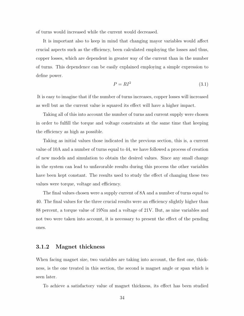
of turns would increased while the current would decreased.
It is important also to keep in mind that changing mayor variables would affect
crucial aspects such as the efficiency, been calculated employing the losses and thus,
copper losses, which are dependent in greater way of the current than in the number
of turns. This dependence can be easily explained employing a simple expression to
define power.
P = RI2 (3.1)
It is easy to imagine that if the number of turns increases, copper losses will increased
as well but as the current value is squared its effect will have a higher impact.
Taking all of this into account the number of turns and current supply were chosen
in order to fulfill the torque and voltage constraints at the same time that keeping
the efficiency as high as possible.
Taking as initial values those indicated in the previous section, this is, a current
value of 10A and a number of turns equal to 44, we have followed a process of creation
of new models and simulation to obtain the desired values. Since any small change
in the system can lead to unfavorable results during this process the other variables
have been kept constant. The results used to study the effect of changing these two
values were torque, voltage and efficiency.
The final values chosen were a supply current of 8A and a number of turns equal to
40. The final values for the three crucial results were an efficiency slightly higher than
88 percent, a torque value of 19Nm and a voltage of 21V. But, as nine variables and
not two were taken into account, it is necessary to present the effect of the pending
ones.
3.1.2 Magnet thickness
When facing magnet size, two variables are taking into account, the first one, thick-
ness, is the one treated in this section, the second is magnet angle or span which is
seen later.
To achieve a satisfactory value of magnet thickness, its effect has been studied
34

following the design methodology employed for most of the variables. It is easy to
come to the conclusion that up to a reasonable value, the bigger the magnet, the
better the results. This is true, in fact the best results were achieved for a value
of 11mm magnet thickness but there is a there is an important reason that advises
against using that size, price.
Given that magnetic materials are usually the most expensive part of the machine,
a new value of 5mm is proposed taking into account a huge change on price but a
minor one in results. Again, there wouldn’t be much difference between selecting 5mm
or a value a bit lower but the chosen one complies well enough with the cost-effective
aspect.
Paying attention to figures 3-1, 3-2 and 3-3, it is possible to see that efficiency,
torque and voltage are at its highest point at the value of 11mm indicated before but
it is also easily seen than the values vary between relatively similar values.
Figure 3-1: Magnet Thickness versus Efficiency
Another factor that advices against selecting a bigger value of magnet thickness
is the possible magnetic saturation present on the stator teeth.
35

Figure 3-2: Magnet Thickness versus Torque
Figure 3-3: Magnet Thickness versus Voltage
3.1.3 Magnet angle
When talking about magnet angle the referred variable can be considered the width
but taking into account that the magnet is located on top of a the rotor surface it is
more convenient to talk about angle.
The value chosen for this variable is based on similar premises than the previous
36
one but in this case saturation comes as even more important than price as it is
necessary to avoid the presence of flux lines ”jumping” between poles.
From the initial value presented in chapter 3, only few modifications have been
needed to select the final one. Been 15 degrees the initial one for the topology and
slot/pole combination under study, 16.5 degrees is the final one. The reason is simply
that above that value flux lines incur in behaviors not wanted due to the increased
proximity between poles.
It is possible to affirm that the bigger the magnets, the better the results within
the range previously described.
3.1.4 Rotor diameter
Given as constraint the outer stator diameter, the value of the inner and thus rotor
diameter is another variable that must be set. Rotor diameter has been selected in
order to maximize the resulting torque. It has been obtained as most suitable a value
of 95mm.
As in most cases and most engineering problems the selection of rotor diameter
is an exchange that must be balanced, this is, if increased a lot, it would reduce the
slot area incurring in possible constraints to the amount of copper conductors which
affects mainly the generated voltage. In case of decreasing it too much, torque will
be dramatically reduced.
3.1.5 Tooth Width Ratio
Tooth width ratio is a characteristic that express the width of the slot teeth with a
value varying from 0 to 1. In reality 0 and 1 are never going to be acceptable values
and real applications will be usually in the range from 0.5 to 0.7.
The main effect of the modification of this variable is the increase or reduction of
the amount of copper conductor as seen on figures 3-4 and 3-5, for this reason, the
smaller the value, the higher the torque and the voltage while, the bigger it is set,
the better the efficiency will be as a reaction of reducing the amount of copper and
37

thus the its main source of losses.
Figure 3-4: Tooth Width Ratio equal to 0.5
Figure 3-5: Tooth Width Ratio equal to 0.7
As it was done for most characteristics, the values were modified and tested for
ten different cases from 0.5 to 0.725 in steps of 0.25. This study pointed out that a
satisfying value could be 0.6 which is the one chosen for the final model. The graphs
summarizing the effect of this changes has been displayed on figures 3-6 and 3-7.
Perhaps this variable stands for the obvious opposition in their graphs where it
can be seen how choosing between one value or another should be taken based on an
election that compromises one of the results. For the case under study, it has been
decided to promote often and up to a maximum value of 20Nm, the torque.
38
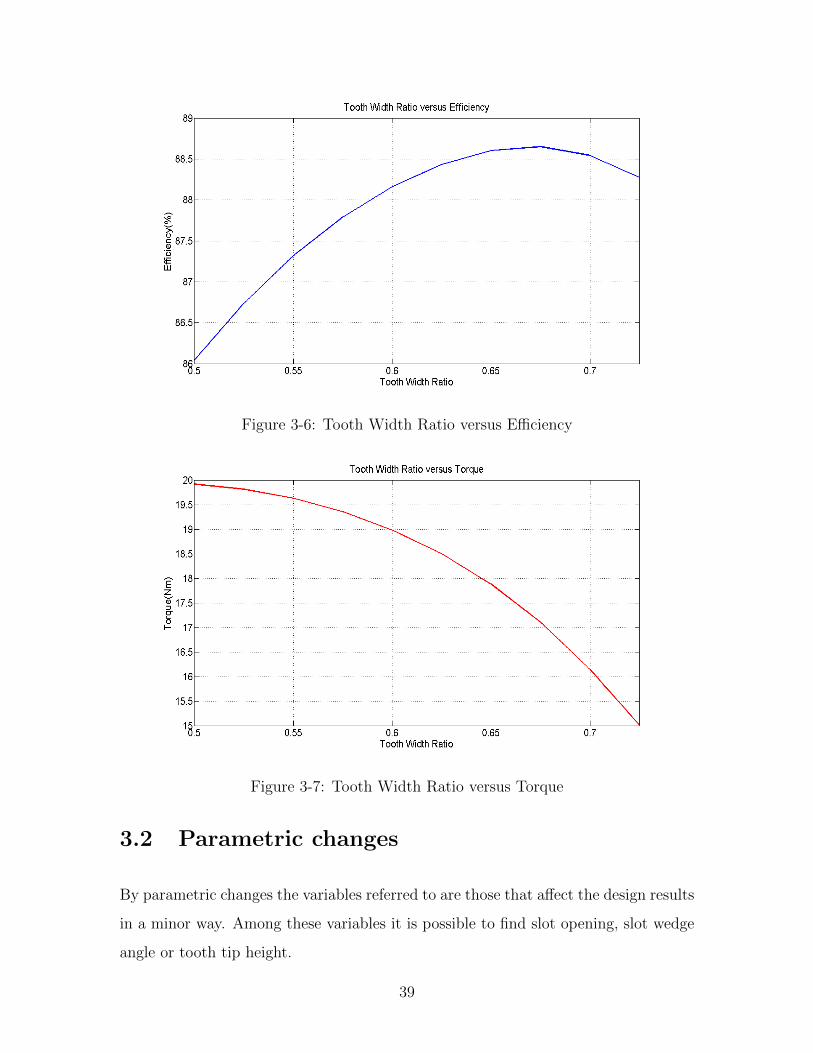
Figure 3-6: Tooth Width Ratio versus Efficiency
Figure 3-7: Tooth Width Ratio versus Torque
3.2 Parametric changes
By parametric changes the variables referred to are those that affect the design results
in a minor way. Among these variables it is possible to find slot opening, slot wedge
angle or tooth tip height.
39
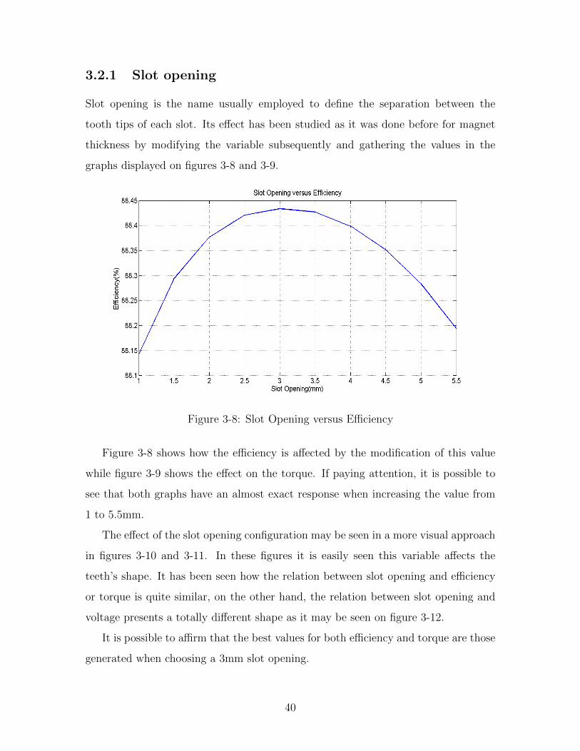
3.2.1 Slot opening
Slot opening is the name usually employed to define the separation between the
tooth tips of each slot. Its effect has been studied as it was done before for magnet
thickness by modifying the variable subsequently and gathering the values in the
graphs displayed on figures 3-8 and 3-9.
Figure 3-8: Slot Opening versus Efficiency
Figure 3-8 shows how the efficiency is affected by the modification of this value
while figure 3-9 shows the effect on the torque. If paying attention, it is possible to
see that both graphs have an almost exact response when increasing the value from
1 to 5.5mm.
The effect of the slot opening configuration may be seen in a more visual approach
in figures 3-10 and 3-11. In these figures it is easily seen this variable affects the
teeth’s shape. It has been seen how the relation between slot opening and efficiency
or torque is quite similar, on the other hand, the relation between slot opening and
voltage presents a totally different shape as it may be seen on figure 3-12.
It is possible to affirm that the best values for both efficiency and torque are those
generated when choosing a 3mm slot opening.
40

Figure 3-9: Slot Opening versus Torque
Figure 3-10: Slot Opening equal to 0.5
3.2.2 Slot wedge angle
Slot wedge angle is a variable that affects visibly the shape of the stator teeth. In
order to illustrate this, figures 3-13 and 3-14 show the huge visual difference that
changing this characteristic may have on the model.
The effect on the results is not so drastic for the range studied, beginning with an
angle of zero degrees and up to forty-five the difference in efficiency is less than one
percent and in torque less than 0.2Nm. It has a noticeable effect in voltage though,
41
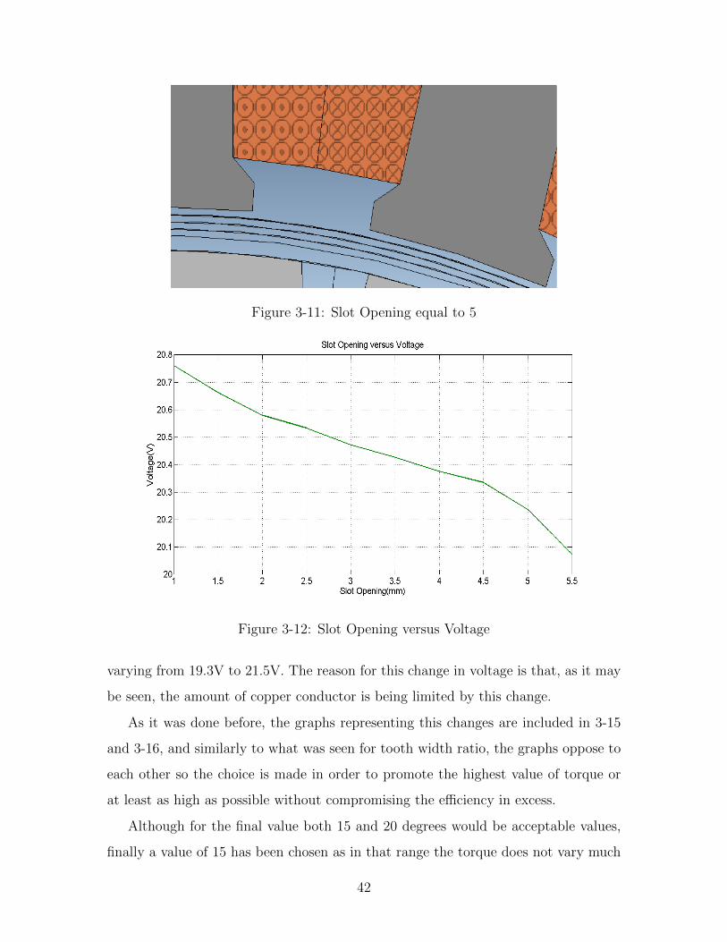
Figure 3-11: Slot Opening equal to 5
Figure 3-12: Slot Opening versus Voltage
varying from 19.3V to 21.5V. The reason for this change in voltage is that, as it may
be seen, the amount of copper conductor is being limited by this change.
As it was done before, the graphs representing this changes are included in 3-15
and 3-16, and similarly to what was seen for tooth width ratio, the graphs oppose to
each other so the choice is made in order to promote the highest value of torque or
at least as high as possible without compromising the efficiency in excess.
Although for the final value both 15 and 20 degrees would be acceptable values,
finally a value of 15 has been chosen as in that range the torque does not vary much
42

Figure 3-13: Slot wedge angle equal to 5
Figure 3-14: Slot wedge angle equal to 35
but the efficiency does.
43

Figure 3-15: Slot Wedge Angle versus Efficiency
Figure 3-16: Slot Wedge Angle versus Torque
3.2.3 Tooth tip height
The variable usually known as tooth tip height hasn’t been studied in detailed as its
modification is often employed as a way to avoid saturation on the teeth tips rather
than to improve in a visible way the results. If increased, the effect seen on the crucial
results is an increase in phase peak voltage but a decreased in torque and efficiency.
44

Decreasing it under the selected value of 1mm is not a good idea either as it would
became a small and fragile edge.
45

46

Chapter 4
Characteristics study
This chapter presents the different characteristics of the machine that have been taken
into account for detailed study seen their importance for the overall performance
during operation.
4.1 Air-gap flux density
Flux density B may be defined as B = µH where H is the magnetic field intensity
and µ the magnetic permeability. Its unit of measurement is the Tesla(T ).
Its behavior can be shown employing the magnetization curve or B-H curve which
shows the magnetic saturation of the different materials, this is, the maximum value
of B that it is possible to achieve.
Regarding the air-gap length, the B −H curve of a magnetic equivalent circuit is
affected by the presence of this air gap in the form that permeability of non-magnetic
material is low so greater values of H are required to obtain the same value of B
compared to magnetic materials. On the other hand, if no air-gap is present then
the slope becomes as steep as possible, and the B −H loop will represent the closest
approximation of the characteristic of the magnetic material. In this case it is not
easy to select an air gap flux density value towards the practical application (design).
Also, due to the increased reluctance of the air gap, the flux spreads into the sur-
rounding medium causing the apparition of non-desired phenomena such as flux fring-
47
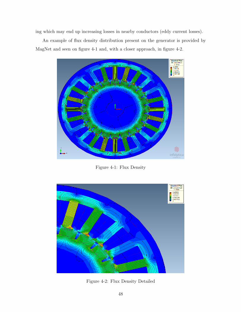
ing which may end up increasing losses in nearby conductors (eddy current losses).
An example of flux density distribution present on the generator is provided by
MagNet and seen on figure 4-1 and, with a closer approach, in figure 4-2.
Figure 4-1: Flux Density
Figure 4-2: Flux Density Detailed
48

Values presented oscillate between 0T for the darkest blues zones and 2.45T for
some small regions which present a slight amount of saturation. The majority of the
colors displayed oscillate around 1T.
Air-gap flux density depends on the MMF, the magnetic boundary conditions, the
length of the air-gap, the effect of the slot openings and the shape of the pole face. It
has two main components, the flux density produced by the stator currents passing
through the windings and the rotor magnets flux density.
It is not an easy task to provide an expression that describes precisely the air-gap
flux density taking into account both components, that is why usually in order to
obtain an approximate value the following equation is employed which takes under
consideration only the component due to the permanent magnets in the rotor. A
good estimation is a value close to 0.9T obtained employing expression 4.1.
Bg =Br
1 + µrLg
Lm
(4.1)
Expression 4.1 perfectly represents the permanent magnet component of the air-
gap flux where Br is the permanent magnet remanent flux equal to 1.1T, µr is the
magnet relative permeability equal to 1.05, Lg is the air-gap length equal to 1mm
and Lm is the magnet length which final chosen value is equal to 5mm.
4.2 Phase flux linkage
Flux linkage is measured in units of weber per turn (Wb/turn) and usually displayed
by the symbol λ. In permanent magnet machines, flux linkage has two clearly dif-
ferentiated components: One due to the permanent magnets remanent flux and the
other due to the flux generated when current circulates through the stator windings
[2]. While obtaining the values through mathematic expressions is rather complex,
getting them employing one of the two software tools described in the design method-
ology is much easier. The software tool employed is MagNet.
The way to obtain each component of the flux linkage consist on calculating the
49

value due to the permanent magnets first, and then subtract it from the total. For
this purpose, a no-load test has been performed by setting to zero amperes the current
sources employed for simulation. The result of doing this has been displayed in figure
4-3, having a maximum value of 0.1702 Wb/turn.
Figure 4-3: Flux Linkage due to Permanent Magnets
Figure 4-4: Total Flux Linkage
All the simulations performed in order to obtain previous and following graphs
50

have been done for an electrical revolution. Total flux linkage obtained by setting the
current sources to the current supply value may bee seen in figure 4-4. It presents a
maximum value of 0.1845 Wb/turn and thus the value for the flux linkage produced
by effect of the currents circulating through the windings is 0.0143 Wb/turn, quite
small if compared with the total, accounting only for 7.75% of it.
For all figures shown previously and in following sections, the number of samples
seen on axis X corresponds also to the time in milliseconds, thus each millisecond, a
new sample is taken. The total number of samples (60) corresponds to one electri-
cal revolution which has been calculated employing the generator frequency seen on
expressions 4.2 and 4.3.
f = ωmp (4.2)
Where ωm is the mechanical speed in rad/s and p is the number of pole pairs.
f =ωrpmpoles
60 · 2=
100 · 20
120= 16.67Hz (4.3)
Once the electrical frequency is known, the total number of milliseconds that must be
simulated is obtained dividing one second or a thousand milliseconds by the frequency,
this is, calculating the period.
T =1000
16.67= 60ms (4.4)
Choosing a total number of sixty time steps, each time step will last a millisecond
and thus sixty samples will be taken.
4.3 Back EMF
Back electromotive force refers to the force produced in a rotating electric machine
by the voltage. That voltage is proportional to the magnetic field, the number of
turns of the windings and the speed of the motor.
Similar to what was done for flux linkage, the best way to obtain the back EMF
51

is to perform a no-load test and look at the voltage results. This has been done
and displayed in figure 4-5. The maximum value obtained is 16.94V for all three
Figure 4-5: Back Electromotive Force
phases. The maximum voltage value obtained if simulating a load test is 21.12V. The
reason why a no load test will point out the value of the back EMF can be explained
with expression 4.3, which shows the different components of which the voltage is
constituted.
V = RI + L
(dI
dt
)+mL
(dI
dt
)+ EMF (4.5)
Where L is the inductance of the windings and mL is the mutual inductance. Thus
if current is set to 0A, the only component for the voltage will be the EMF and then
the software employed will provide the previous results [3].
4.4 Torque
4.4.1 Average torque
Average torque can be calculated employing the results provided by MagNet through
simulation. In figure 4-6 torque has been displayed with a maximum value of 19.13Nm
52

and a minimum of 18.86Nm.
Figure 4-6: Torque
From the data that form 4-6 it is possible to obtain that the average Torque value
is 18.9826Nm.
4.4.2 Cogging torque
Cogging torque is the torque produced due to the interaction between the magnets
flux and the stator slots of a permanent magnet machine. It is a non-desired position
dependent component of the torque which is especially prejudicial at low speeds. The
task of analytical calculation and minimization of the cogging torque in PM machines
is typically accomplished using Maxwell stress tensor methods [5].
The way to obtain it through MagNet simulation is by performing a no-load test
which allows looking at the torque produced by the configuration of the machine, this
is, the inherent torque of the device without taken into consideration supply current
or any other variable.
Figure 4-7 shows the graph for the cogging torque provided by MagNet where it
is possible to see that the values oscillate around zero from a minimum of -0.015Nm
to a maximum of 0.01Nm.
53

Figure 4-7: Cogging Torque
4.4.3 Torque ripple
Torque ripple is the periodic increase or decrease in output torque during the rotation
of an electric machine usually expressed as a percentage of the total.
Among the possible sources of torque ripple, the main ones are the difference in
amplitude in phase back-EMF or currents, the phase offset deviation between phases
and the presence of harmonic components.
For the first case, and considering the amplitude of the back-EMF or the current
in phase A to be a factor of (1+∆) greater than ideal, the torque will be as seen on
expression 4.4.3 and 4.4.3.
T (θ) = KpIp[(1 + ∆)cos2(θ) + cos2(θ − θph) + cos2(θ + θph)] (4.6)
T (θ) =3 + ∆
2KpIp +
∆
2KpIpcos(2θ) (4.7)
Then, as the constant torque produced has increased to (3+∆) KpIp/2 and a torque
ripple term at the second harmonic of the fundamental electrical frequency appears
with amplitude ∆KpIp/2, the ratio of the amplitude of the torque ripple to the
54

constant torque produced is:∆
3 + ∆≈ ∆
3(4.8)
Using this approximation a 3% amplitude error in one phase produces a peak torque
ripple of approximately 1% [3]. If looking at the second source of torque stated at
the beginning of this section, when the phase offset of a back-EMF or current shape
deviates from the ideal, it is possible to obtain that a mere 0.03rad(≈ 1.72◦) phase
misalignment produces 1% peak torque ripple. The third possibility is not easily
obtained as it is subject to harmonic content.
For the case under study and going back to the results obtained from MagNet,
torque ripple can be easily spotted on figure 4-6 previously shown. The difference
between the lower and the upper peaks is 0.2651Nm which represents approximately
1.4% of the total.
4.5 Current density
In electromagnetism current density is defined as the electric current per cross sec-
tional unit area and usually displayed as “J”. It is defined as a vector whose mag-
nitude is the electric current per cross-sectional area at a given point in space. In
SI units, the electric current density is measured in amperes per square meter but
usually employed as amperes per square millimeter.
Current density together with the electrical loading plays a crucial role in the
thermal criterion and calculation of the temperature rise during operation of electrical
machines. For naturally cooled machines like the case under study the typical value
for current density is around 4A/mm2. A common expression to define current density
is the one that relates it to the electrical loading “A”, the slot area “Aslot”, the slot-fill
factor “Fslot” and the slot pitch “λ”. It has been shown in expression (4.5). This
equation can be also related to the slot-depth “d” and the tooth width “t” [6].
J =Aλ
FslotAslot=
A
Fslotd(1− τ)(4.9)
55
Where τ=t/λ, and A is described by expression 4.5.
A =2mNphIrms
πD(4.10)
Where m is the number of phases, Nph is number of turns per phase, Irms is the supply
current effective value and D is the stator outer diameter. Substituting everything
on the previous expression leads to solved equation 4.5.
A =2 · 3 · 320 · 8/
√2
π · 155 · 10−3= 22.3 · 103 (4.11)
Once the current loading is known, it is possible to go back to expression 4.5, sub-
stitute all values and obtain the current density analytical value seen in 4.5.
J =22.3 · 103
0.5 · 23(1− 6.48
12.43
) = 4.05A/mm2 (4.12)
Obtaining a value very close to 4A/mm2 which as it was said before is in the common
range for this kind of machines.
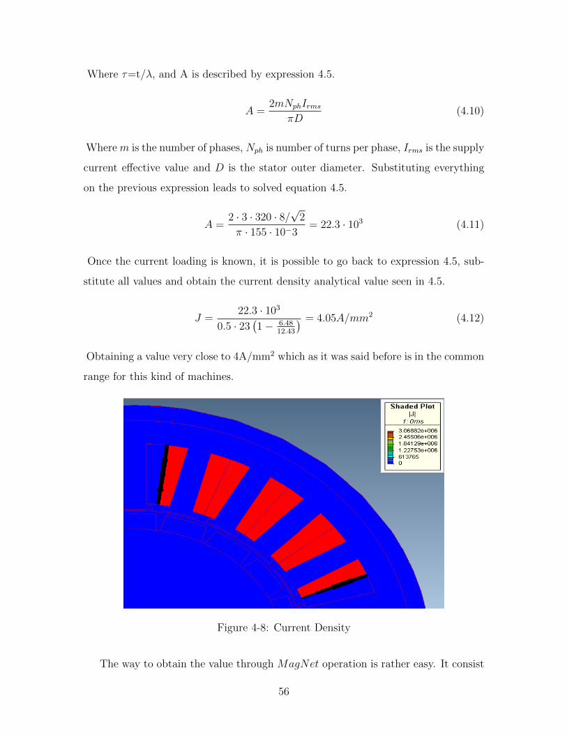
Figure 4-8: Current Density
The way to obtain the value through MagNet operation is rather easy. It consist
56

on measuring the value for the current density in the point of operation where the
waveform of the current supply is at 90 degrees which corresponds to the time instant
at 15 milliseconds and then multiplying that value by two and dividing it by π.
Finally, as MagNet wasn’t taking into account the winding factor which is 50%, it is
necessary to multiply the final value by two again.
If looking at figure 4-8, it is possible to see that the value is 3.0688A/mm2.
Then following the process previously described it is possible to obtain a value of
3.9073A/mm2 which is not far from the one calculated analytically.
4.6 Copper Losses
Copper loss refers to the wasted energy in form of heat produced by electrical currents
in conductors. The term is applied regardless of whether the windings are made of
copper or another conductor, such as aluminum. The term load loss is closely related
but not identical, since an unloaded transformer will have some winding loss.
Figure 4-9: Half Slot Copper Losses
Regarding copper losses, the obtainment of results from MagNet is an automatic
process as they are among the values provided right after simulating. The value of
57

ohmic losses for a single layer of slot (double layer side-by-side windings) may be seen
in graphical form in figure 4-9.
From the values shown in figure 4-9 it is possible to obtain the total average value
of copper losses by obtaining the average of those values employed to draw the curve,
multiply it by two to obtain the losses of each slot and then multiply it by twenty-four
to obtain the total value which in the case under study is 25.3769W.
It is also possible to obtain copper or ohmic losses through analytical expressions
which on its simplest form are described as it was seen on model optimization and
also in equation 4.6.
Pcopper = RI2 (4.13)
The problem is that obtaining the resistance value depends on a far more complicated
expression seen on 4.6.
R =2ρcuLNphI
2rms
(pq)AslotFslot(4.14)
Where ρcu stands for electrical resistivity of copper, L = (Pa + Psl)N2ph been Pa
the air-gap permeance and Psl the slot leakage permeance, Nph is the number of turns
per phase, I2rms is the effective value of the current supply, p is the number of pole
pairs, q = Ns/(m · 2p) been Ns the number of slots and m total number of phases,
Aslot is the slot area and Fslot is the slot-fill factor.
In short, it is not worth using the equation as it would be necessary to take
some characteristics from the software model due to the absence of a more complex
analytical model.
4.7 Iron Losses
Iron losses also known as core losses are a result of the effect produced by the varying
magnetic field induced by the alternating current passing through the windings on
the core which makes some of the power dissipate as heat or noise. There are mainly
two processes involved in this loss, hysteresis and eddy currents.
58

Analytically, iron losses can be obtained employing the expression known as Stein-
metz’s loss which has been displayed in 4.7. It is formed by two components, the first
one due to hysteresis and the second one due to eddy current losses. It provides values
in W/kg.
Piron = khfαBβ + ke(sfB)2 (4.15)
Where kh and ke are the hysteresis and eddy current constants, f is the current
supply frequency, B is the peak flux density, and s is the lamination thickness ratio.
All these values are provided and employed by MagNet for each material present on
the software [7].
In practice it is not necessary to look for these values as iron losses for both stator
yoke and rotor core are provided by MagNet automatic simulation results in time
averaged form separated into hysteresis and eddy current losses.
4.7.1 Hysteresis
The varying magnetic field through the core changes the magnetization of its material
producing a process of expansion and contraction which causes losses in form of heat.
This process known as hysteresis loss can be seen in the material B-H loop.
For the case under study stator yoke hysteresis losses are 1.2629W while for the
rotor core are 1.2702mW.
4.7.2 Eddy Current
Eddy currents losses are a result of the electric resistance of the core material to
the circulating currents produced by the varying magnetic fields. That resistance
dissipates part of the power in form of heat. The power loss is proportional to the
area of the loops and inversely proportional to the resistivity of the core material [8].
For the final chosen model, eddy current losses are 49.6397mW for the stator and
0.0284mW for the rotor. It is possible to affirm that both values from eddy current
losses and in general, values from rotor iron losses are negligible when compared to
stator yoke hysteresis losses.
59

Magnets
Losses in the magnets are caused by eddy-currents which as it was briefly explained
before are due to the variation of flux-density in the magnets. The process is exactly
the same as the generation of eddy-currents in general.
With respect to eddy currents in the magnets a way to calculate it is by looking
at the ohmic losses in the magnets provided by MagNet. Looking at the values from
the 20 poles seen in figure 4-10 it is possible to affirm that the average losses for
this specific element are around 0.58mW. The maximum value reached among all the
data collected was 1.44mW. It is easy to see that figure 4-10 represents two magnets
Figure 4-10: Magnet Eddy Current Losses
that for being immediately close to each other are shifted 90 degrees, in other words,
one pole is facing one direction and the next one is facing the opposite in order to
achieve that varying magnetic field responsible for the generation of electricity in the
windings.
Sleeve
Mainly produced by the higher space harmonics due to slot openings; however, in the
case of full-pitch stator winding, other space harmonics can also be significant.
60

Regarding the sleeve eddy current losses, for the case under study the sleeve
material considered was air then they were not eddy currents involved in this part of
the machine. For a more realistic application the sleeve material should be changed
to carbon fiber for instance and new simulations should be carried out in order to
obtain values from the model.
4.8 Demagnetization and variation with tempera-
ture
The study of demagnetization in a permanent magnet motor or generator can be done
by looking at how two variables change according to a temperature difference. Those
variables, explained below, are remanent flux density and coercivity.
4.8.1 Remanent flux density
Been “Br” the remanent flux-density, its demagnetization is specified in terms of
“αBr” which stands for reversible temperature coefficient of “Br” expressed in per-
centage per Celsius degree.
Br(t◦) = Br(20◦C)
[1 + αBr
t◦ − 20
100
](4.16)
Where Br(20◦C) is 1.1T, the value of Br at 20◦C, usual value for room temperature.
The coefficient alphaBr is around -0.09 -0.15%/◦C in the case of neodymium iron
boron magnets. In order to try this behavior a temperature of 60◦C is chosen as
maximum machine temperature under operation to observe the demagnetization:
Br(t◦) = 1.1
[1− 0.12
60− 20
100
]= 1.0472T (4.17)
It is possible to see that the remanent flux-density does not vary significantly for that
temperature difference giving this material good behavior when referring to “Br”.
61

4.8.2 Coercivity
Coercivity (Hc) is a measure of a ferromagnetic or ferroelectric material to withstand
an external magnetic or electric field. For ferromagnetic material the coercivity is the
intensity of the applied magnetic field required to reduce the magnetization of that
material to zero after the magnetization of the sample has been driven to saturation.
Thus coercivity measures the resistance of a ferromagnetic material to becoming
demagnetized.
When referring to “Hc” the temperature coefficient is between -0.4 and -0.8
”%”/◦C [9]. This will cause a significant change in coercivity during operation.
Hc(t◦) = Hc(20◦C)
[1 + αHc
t◦ − 20
100
](4.18)
The coercivity of neodymium iron boron magnets at room temperature according
to MagNet is 827.6kA/m. Then the value obtained for the same temperature used
before can be seen in expression (4.8.2).
Hc(t◦) = 827.6 · 103
[1− 0.6
60− 20
100
]= 628.98kA/m (4.19)
As it was said before, the coercivity of neodymium iron boron magnets varies in a
much greater way than the remanent flux density.
4.9 Radial forces
Permanent magnet machines are subject to great sources of vibration forces been
them mainly radial forces and unbalanced magnetic forces. Taking into account
the existence of rotor eccentricity, these forces are increased due to mechanical and
magnetic coupling effects [10].
Regarding radial force, it is possible to obtain it in an oversimplified way as the
product of the previously obtained torque multiplied by the velocity or linear speed.
Knowing that the angular speed is 100rpm or 10.47rad/s and the rotor outer diameter
62
is 95mm, it is possible to obtain it as v =ω·r , and then the linear speed is equal to
0.99m/s.
Once the linear speed is known and assuming it is constant, the radial force may
be calculated with the 60 measurements (or sample points) of motion rotor torque
provided by MagNet.
The average force obtained from the total number of measurements is 18.79N. It is
not displayed here as it looks exactly like the torque graphical representation shown
in figure 4-6 with every value multiplied by 0.99.
63

64

Chapter 5
Conclusion
The market for electric bicycles is seeing a boom which has not seen on its history
before and that is why through constant innovation it will be allowed to increase and
maintain the interest of users promoting the use of these vehicles and thus contributing
positively to an improvement of the environment as well as people’s quality of life.
It is possible to state firmly that the project objectives have been completely
fulfilled, as it has provided a final model of electric generator that complies with
design constraints, that will be manufactured in the near future and used as first
prototype in a much larger project consisting on creating the chain-less electric bicycle
described in the introduction.
Final characteristics achieved through model optimization and further analysis
satisfy well enough design constraints, these and the results have been summarize in
tables 5.1 and 5.2 respectively.
5.1 Future Work
The final model provided by this project accounts for the first prototype of generator
which will be used as a start point for further improvement and for intensive testing
previous to its implementation on a market product. As it was said on the intro-
duction, this project is included within a much larger one that will comprise a whole
electric bicycle, therefore and in this sense, there is still a large backlog in regard to
65
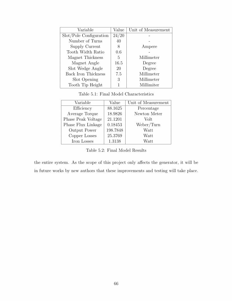
Variable Value Unit of MeasurementSlot/Pole Configuration 24/20 -
Number of Turns 40 -Supply Current 8 Ampere
Tooth Width Ratio 0.6 -Magnet Thickness 5 Millimeter
Magnet Angle 16.5 DegreeSlot Wedge Angle 20 Degree
Back Iron Thickness 7.5 MillimeterSlot Opening 3 Millimeter
Tooth Tip Height 1 Millimiter
Table 5.1: Final Model Characteristics
Variable Value Unit of MeasurementEfficiency 88.1625 Percentage
Average Torque 18.9826 Newton MeterPhase Peak Voltage 21.1201 VoltPhase Flux Linkage 0.18453 Weber/Turn
Output Power 198.7848 WattCopper Losses 25.3769 Watt
Iron Losses 1.3138 Watt
Table 5.2: Final Model Results
the entire system. As the scope of this project only affects the generator, it will be
in future works by new authors that these improvements and testing will take place.
66

Bibliography
[1] S.E.Skaar, Ø. Krøvel, R. Nilssen, ”Distribution, coil-span and winding factors forPM machines with concentrated windings”.
[2] A.E. Fitzgerald, Charles Kingsley, Jr., Stephen D. Umans, “Electric Machinery,Sixth Edition”, New York, 2003.
[3] Dr. Duane Hanselman, “Brushless Permanent Magnet Motor Design, Second Edi-tion”, Electrical and Computer Engineering, University of Maine, Orono, USA,2006.
[4] Stanely Humphries, “Tutorial: Surface integral expressions for electric/magneticforce and torque”, Field Precision, 2012.
[5] Ayman M. El-Refaie, Thomas M. Jahns, Donald W. Novotny, “Analysis of SurfacePermanent Magnet Machines with Fractional-Slot Concentrated Windings”, IEEETransactions on energy conversion, vol. 21, no. 1, March 2006.
[6] TJE Miller, “SPEED’s Electric Machines”, University of Glasgow, Department ofElectronics and Electrical Engineering, 2002-2011.
[7] Jacek F. Gieras, Andreas C. Koenig, Laurence D. Vanek, “Calculation of EddyCurrent Losses in Conductive Sleeves of Synchronous Machines”, Proceedings ofthe 2008 International Conference on Electrical Machines.
[8] H. Polinder, M.J. Hoeijmakers, M. Scuotto, “Eddy-Current Losses in the SolidBack-Iron of PM Machines for different Concentrated Fractional Pitch Windings”,Electrical Power Processing, Delft University of Technology, The Netherlands,2007.
[9] Jacek F. Gieras, Rong-Jie Wang, Maarten J. Kamper, ”Axial Flux PermanentMagnet Brushless Machines, 2nd Edition”, 2008.
[10] Kyung-Tae K., Kwang-Suk K., Sang-Moon H., Tae-Jong K., Yoong-Ho J., ”Com-parison of Magnetic Forces for IPM and SPM Motor with Rotor Eccentricity”,IEEE Transactions on magnetics, vol. 37, no. 5, September 2001.
67