High Dimensional Linear Algebra

1

10-606 Mathematical Foundations for Machine Learning

Matt GormleyLecture 6

September 17, 2018

Machine Learning DepartmentSchool of Computer ScienceCarnegie Mellon University

Q&A

3

HEBIAN LEARNING &MATRIX MEMORIES

4

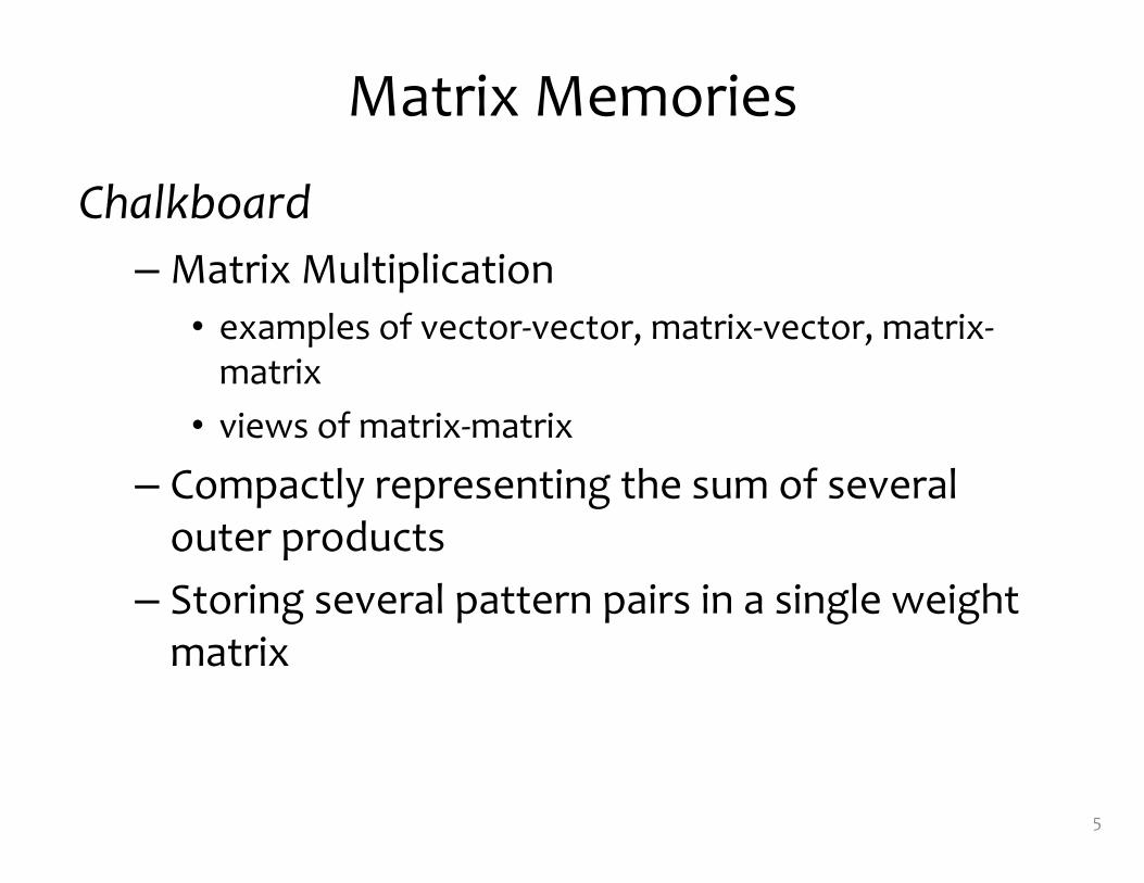
Matrix Memories

Chalkboard– Matrix Multiplication

• examples of vector-vector, matrix-vector, matrix-matrix

• views of matrix-matrix

– Compactly representing the sum of several outer products

– Storing several pattern pairs in a single weight matrix

5

Ex: Matrix Memories in Numpy

6

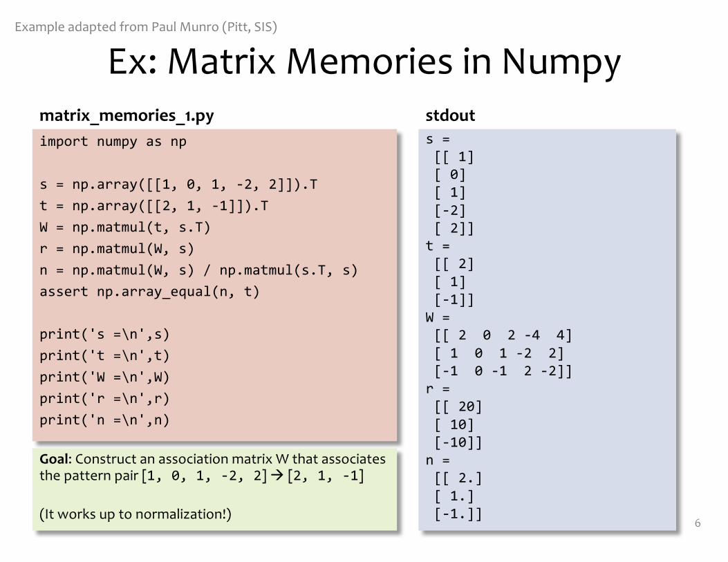
import numpy as np

s = np.array([[1, 0, 1, -2, 2]]).Tt = np.array([[2, 1, -1]]).TW = np.matmul(t, s.T)r = np.matmul(W, s)n = np.matmul(W, s) / np.matmul(s.T, s)assert np.array_equal(n, t)

print('s =\n',s)print('t =\n',t)print('W =\n',W)print('r =\n',r)print('n =\n',n)

s = [[ 1] [ 0] [ 1] [-2] [ 2]] t = [[ 2] [ 1] [-1]] W = [[ 2 0 2 -4 4] [ 1 0 1 -2 2] [-1 0 -1 2 -2]] r = [[ 20] [ 10] [-10]] n = [[ 2.] [ 1.] [-1.]]

matrix_memories_1.py stdout

Goal: Construct an association matrix W that associates the pattern pair [1, 0, 1, -2, 2] à [2, 1, -1]

(It works up to normalization!)

Example adapted from Paul Munro (Pitt, SIS)

Ex: Matrix Memories in Numpy

7

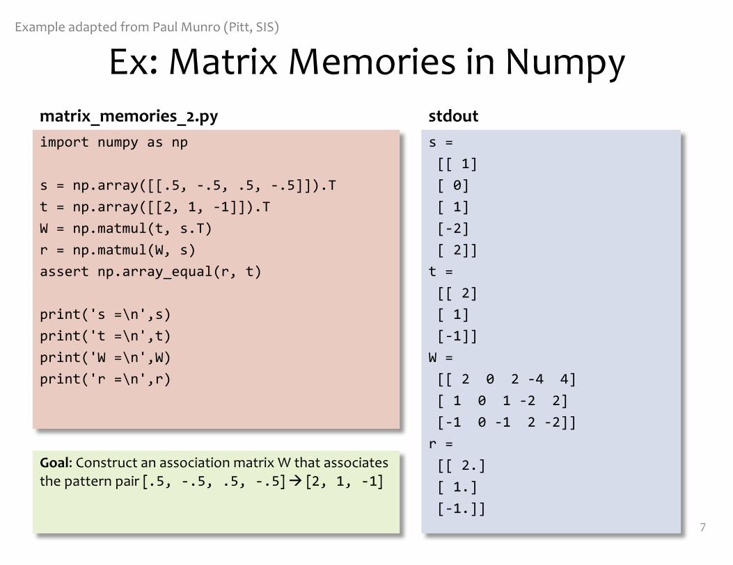
import numpy as np

s = np.array([[.5, -.5, .5, -.5]]).T t = np.array([[2, 1, -1]]).T W = np.matmul(t, s.T) r = np.matmul(W, s) assert np.array_equal(r, t) print('s =\n',s) print('t =\n',t) print('W =\n',W) print('r =\n',r)

s = [[ 1] [ 0] [ 1] [-2] [ 2]] t = [[ 2] [ 1] [-1]] W = [[ 2 0 2 -4 4] [ 1 0 1 -2 2] [-1 0 -1 2 -2]] r = [[ 2.] [ 1.] [-1.]]

stdoutmatrix_memories_2.py

Goal: Construct an association matrix W that associates the pattern pair [.5, -.5, .5, -.5] à [2, 1, -1]

Example adapted from Paul Munro (Pitt, SIS)

Ex: Matrix Memories in Numpy

8

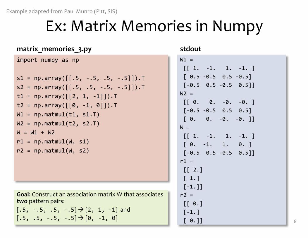
import numpy as np

s1 = np.array([[.5, -.5, .5, -.5]]).Ts2 = np.array([[.5, .5, -.5, -.5]]).Tt1 = np.array([[2, 1, -1]]).Tt2 = np.array([[0, -1, 0]]).TW1 = np.matmul(t1, s1.T)W2 = np.matmul(t2, s2.T)W = W1 + W2r1 = np.matmul(W, s1)r2 = np.matmul(W, s2)

W1 = [[ 1. -1. 1. -1. ] [ 0.5 -0.5 0.5 -0.5] [-0.5 0.5 -0.5 0.5]] W2 = [[ 0. 0. -0. -0. ] [-0.5 -0.5 0.5 0.5] [ 0. 0. -0. -0. ]] W = [[ 1. -1. 1. -1. ] [ 0. -1. 1. 0. ] [-0.5 0.5 -0.5 0.5]] r1 = [[ 2.] [ 1.] [-1.]] r2 = [[ 0.] [-1.] [ 0.]]

stdoutmatrix_memories_3.py

Goal: Construct an association matrix W that associates two pattern pairs: [.5, -.5, .5, -.5] à [2, 1, -1] and[.5, .5, -.5, -.5] à [0, -1, 0]

Example adapted from Paul Munro (Pitt, SIS)

Ex: Matrix Memories in Numpy

9

import numpy as np

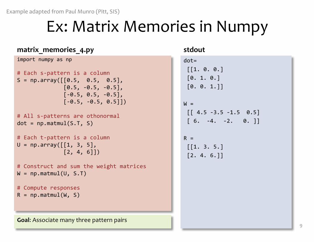
# Each s-pattern is a columnS = np.array([[0.5, 0.5, 0.5],

[0.5, -0.5, -0.5],[-0.5, 0.5, -0.5],[-0.5, -0.5, 0.5]])

# All s-patterns are othonormaldot = np.matmul(S.T, S)

# Each t-pattern is a columnU = np.array([[1, 3, 5],

[2, 4, 6]])

# Construct and sum the weight matricesW = np.matmul(U, S.T)

# Compute responsesR = np.matmul(W, S)

dot= [[1. 0. 0.] [0. 1. 0.] [0. 0. 1.]] W = [[ 4.5 -3.5 -1.5 0.5] [ 6. -4. -2. 0. ]] R = [[1. 3. 5.] [2. 4. 6.]]

stdoutmatrix_memories_4.py

Goal: Associate many three pattern pairs

Example adapted from Paul Munro (Pitt, SIS)

Ex: Matrix Memories in Numpy

10

import numpy as np

# Each s-pattern is a columnS = np.array([[0.5, 0.5, 0.5],

[0.5, -0.5, -0.5],[-0.5, 0.5, -0.5],[-0.5, -0.5, 0.5]])

# All s-patterns are othonormaldot = np.matmul(S.T, S)

# Each t-pattern is a columnU = np.array([[1, 3, 5],

[2, 4, 6]])

# Construct and sum the weight matricesW = np.matmul(U, S.T)

# Compute responsesR = np.matmul(W, S)

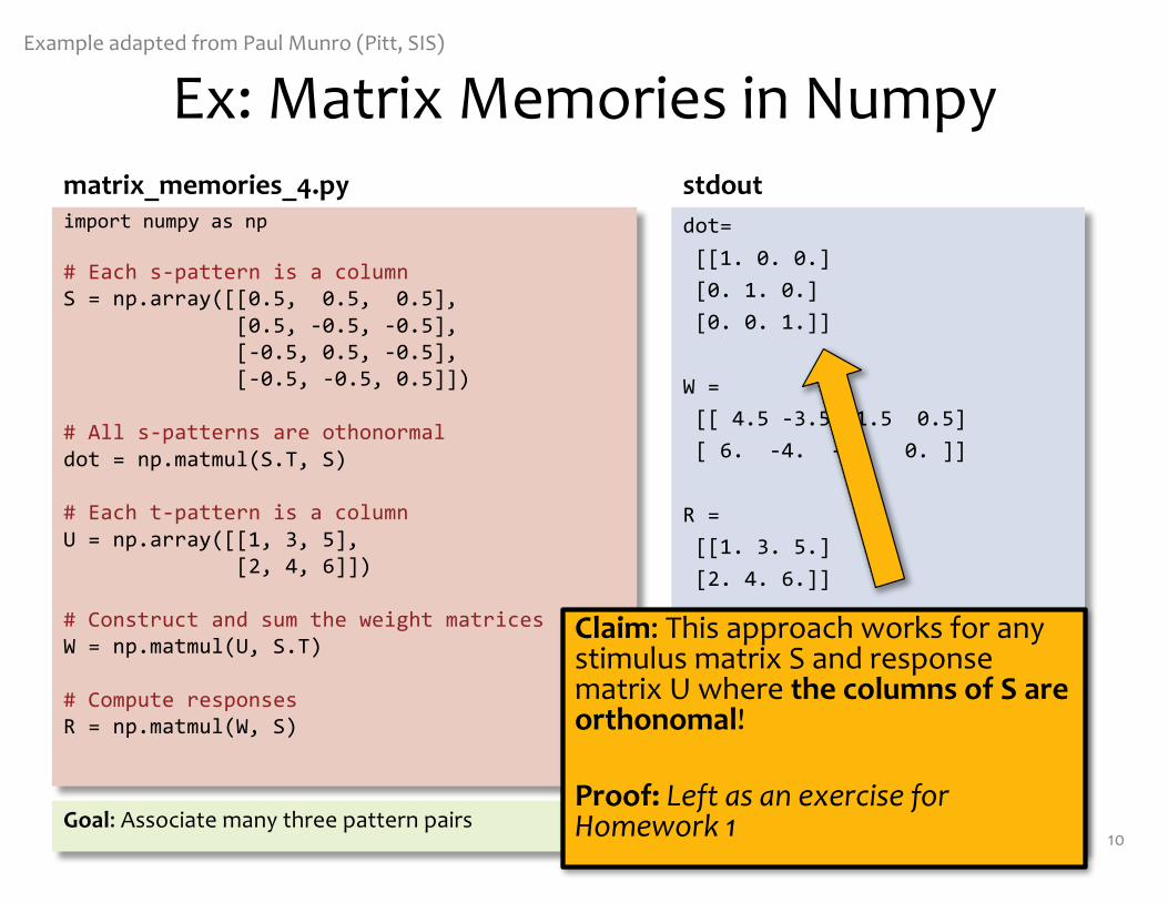
dot= [[1. 0. 0.] [0. 1. 0.] [0. 0. 1.]] W = [[ 4.5 -3.5 -1.5 0.5] [ 6. -4. -2. 0. ]] R = [[1. 3. 5.] [2. 4. 6.]]

stdoutmatrix_memories_4.py

Goal: Associate many three pattern pairs

Example adapted from Paul Munro (Pitt, SIS)

Claim: This approach works for any stimulus matrix S and response matrix U where the columns of S are orthonomal!

Proof: Left as an exercise for Homework 1

MATRIX MEMORIES & APPROXIMATE RECOVERY

17

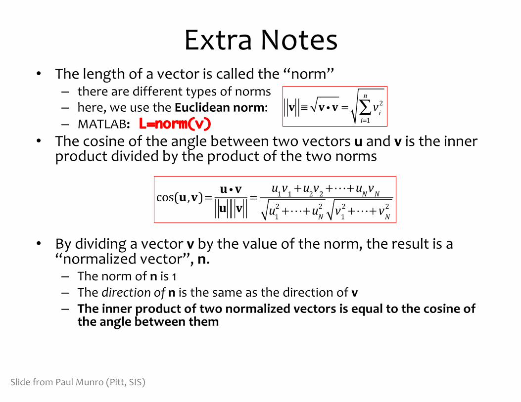
Extra Notes• The length of a vector is called the “norm”

– there are different types of norms– here, we use the Euclidean norm:– MATLAB: L=norm(v)

• The cosine of the angle between two vectors u and v is the inner product divided by the product of the two norms

• By dividing a vector v by the value of the norm, the result is a “normalized vector”, n.– The norm of n is 1– The direction of n is the same as the direction of v – The inner product of two normalized vectors is equal to the cosine of

the angle between them

v ≡ v iv = vi

2

i=1

n

∑

cos(u ,v)= u iv

u v=

u1v1 +u2v2 +!+uNvNu12 +!+uN

2 v12 +!+ vN

2

Slide from Paul Munro (Pitt, SIS)

Slide from Paul Munro (Pitt, SIS)

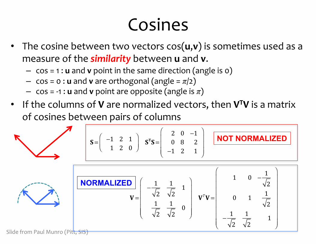
Cosines• The cosine between two vectors cos(u,v) is sometimes used as a

measure of the similarity between u and v.– cos = 1 : u and v point in the same direction (angle is 0)– cos = 0 : u and v are orthogonal (angle = π/2)– cos = -1 : u and v point are opposite (angle is π)

• If the columns of V are normalized vectors, then VTV is a matrix of cosines between pairs of columns

S = −1 2 11 2 0

⎛

⎝⎜⎞

⎠⎟STS =

2 0 −10 8 2

−1 2 1

⎛

⎝

⎜⎜⎜

⎞

⎠

⎟⎟⎟

V =− 1

212

1

12

12

0

⎛

⎝

⎜⎜⎜⎜⎜

⎞

⎠

⎟⎟⎟⎟⎟

VTV =

1 0 − 12

0 1 12

− 12

12

1

⎛

⎝

⎜⎜⎜⎜⎜⎜⎜⎜

⎞

⎠

⎟⎟⎟⎟⎟⎟⎟⎟

NOT NORMALIZED

NORMALIZED

Cosines (cont)

S = −1 2 11 2 0

⎛

⎝⎜⎞

⎠⎟STS =

2 0 −10 8 2

−1 2 1

⎛

⎝

⎜⎜⎜

⎞

⎠

⎟⎟⎟

V =− 1

212

1

12

12

0

⎛

⎝

⎜⎜⎜⎜⎜

⎞

⎠

⎟⎟⎟⎟⎟

VTV =

1 0 − 12

0 1 12

− 12

12

1

⎛

⎝

⎜⎜⎜⎜⎜⎜⎜⎜

⎞

⎠

⎟⎟⎟⎟⎟⎟⎟⎟

NOT NORMALIZED

NORMALIZED

s(1) s(2) s(3)

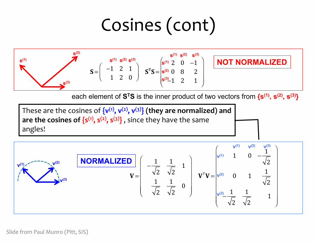
each element of STS is the inner product of two vectors from {s(1), s(2), s(3)}

s(1) s(2) s(3)

s(1)s(2)

s(3) s(3)

s(2)

s(1)

v(1) v(2)

v(3)

These are the cosines of {v(1), v(2), v(3)} (they are normalized) and are the cosines of {s(1), s(2), s(3)} , since they have the same angles!

v(1) v(2) v(3)

v(1)

v(2)

v(3)

Slide from Paul Munro (Pitt, SIS)

High Dimensional Vectors

21

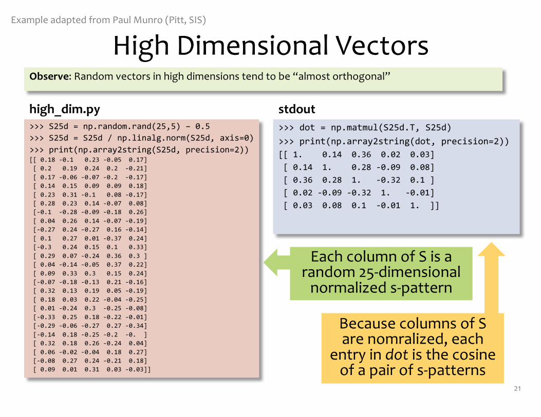
>>> S25d = np.random.rand(25,5) – 0.5>>> S25d = S25d / np.linalg.norm(S25d, axis=0)>>> print(np.array2string(S25d, precision=2))[[ 0.18 -0.1 0.23 -0.05 0.17][ 0.2 0.19 0.24 0.2 -0.21][ 0.17 -0.06 -0.07 -0.2 -0.17][ 0.14 0.15 0.09 0.09 0.18][ 0.23 0.31 -0.1 0.08 -0.17][ 0.28 0.23 0.14 -0.07 0.08][-0.1 -0.28 -0.09 -0.18 0.26][ 0.04 0.26 0.14 -0.07 -0.19][-0.27 0.24 -0.27 0.16 -0.14][ 0.1 0.27 0.01 -0.37 0.24][-0.3 0.24 0.15 0.1 0.33][ 0.29 0.07 -0.24 0.36 0.3 ][ 0.04 -0.14 -0.05 0.37 0.22][ 0.09 0.33 0.3 0.15 0.24][-0.07 -0.18 -0.13 0.21 -0.16][ 0.32 0.13 0.19 0.05 -0.19][ 0.18 0.03 0.22 -0.04 -0.25][ 0.01 -0.24 0.3 -0.25 -0.08][-0.33 0.25 0.18 -0.22 -0.01][-0.29 -0.06 -0.27 0.27 -0.34][-0.14 0.18 -0.25 -0.2 -0. ][ 0.32 0.18 0.26 -0.24 0.04][ 0.06 -0.02 -0.04 0.18 0.27][-0.08 0.27 0.24 -0.21 0.18][ 0.09 0.01 0.31 0.03 -0.03]]

>>> dot = np.matmul(S25d.T, S25d)>>> print(np.array2string(dot, precision=2))[[ 1. 0.14 0.36 0.02 0.03][ 0.14 1. 0.28 -0.09 0.08][ 0.36 0.28 1. -0.32 0.1 ][ 0.02 -0.09 -0.32 1. -0.01][ 0.03 0.08 0.1 -0.01 1. ]]

stdouthigh_dim.py

Observe: Random vectors in high dimensions tend to be “almost orthogonal”

Example adapted from Paul Munro (Pitt, SIS)

Because columns of S are nomralized, each

entry in dot is the cosine of a pair of s-patterns

Each column of S is a random 25-dimensional

normalized s-pattern

High Dimensional Vectors

22

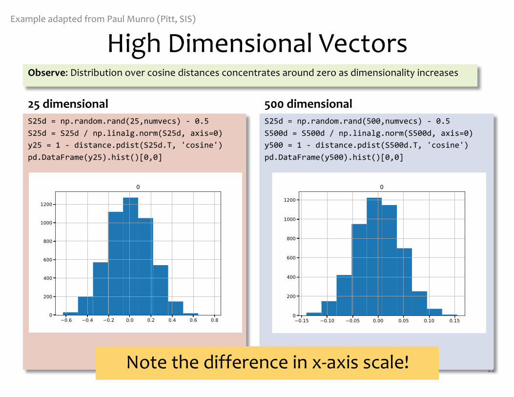
S25d = np.random.rand(25,numvecs) - 0.5S25d = S25d / np.linalg.norm(S25d, axis=0)y25 = 1 - distance.pdist(S25d.T, 'cosine')pd.DataFrame(y25).hist()[0,0]

S25d = np.random.rand(500,numvecs) - 0.5S500d = S500d / np.linalg.norm(S500d, axis=0)y500 = 1 - distance.pdist(S500d.T, 'cosine')pd.DataFrame(y500).hist()[0,0]

500 dimensional25 dimensional

Observe: Distribution over cosine distances concentrates around zero as dimensionality increases

Example adapted from Paul Munro (Pitt, SIS)

Note the difference in x-axis scale!

Using log(x)

1 2 30

0.2

0.4

0.6

0.8

25D 500D 10000D 1 2 3

-15

-10

-5

0

25D 500D 10000D

1 2 3

-6

-4

-2

0

25D 500D 10000D

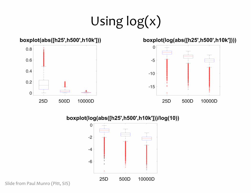
boxplot(log(abs([h25',h500',h10k'])))

boxplot(log(abs([h25',h500',h10k']))/log(10))

boxplot(abs([h25',h500',h10k']))

Slide from Paul Munro (Pitt, SIS)

LINEAR ALGEBRA

29

Linear Algebra: MatricesChalkboard

– Types of Matrices• square matrix• diagonal matrix• identity matrix• symmetric matrix (and the set of symmetric matrices)• orthogonal matrix (different than orthogonal vectors!)

– Matrix Operations• The Transpose• The Trace• Inverse• Determinant

30

Linear Algebra: Linear Independence

Chalkboard– Linear Independence

• Linear combinations of vectors• Linear independence/dependence• Rank: column rank, row rank, full rank• Full rank à invertible

31

Linear Algebra + Matrix Memories

Chalkboard– Intuition: why Matrix Memories work– Intuition: invertible Matrix Memories and

geometry

32