Yeast understanding basic life functions 11,904 p-values Blomberg et al. 2003, 2010

Arabidopsis Thaliana association mapping 3,745 p-values Zhao et al. 2007

fMRI brain scans function of brain language network appr. 3 mill. p-values Taylor et al. 2006

High-dimensional data analysis, fall 2013

TexPoint fonts used in EMF.

Read the TexPoint manual before you delete this box.: AA

1

The course

• Lasso - linear models - generalized linear models - group - smooth functions • P-values • Boosting (perhaps) • Graphical models • Asymptotics

Course book: “Statistics for High-Dimensional Data. Methods, Theory and Applications”, P. Buhlmann and S. van de Geer, Springer 2011.

Complementary book: ”The Elements of Statistical Learning”, T. Hastie, R. Tibshirani, J. Friedman, Springer 2009

Slides for B&vdG 1-2.7: Lasso

Exercises: 2.1, 2.2. 2.3

B&vdG 2.2

Simplest case:

𝑌1 = 𝑋1(1)

𝛽1 + 𝑋1(2)

𝛽2 + ⋯ 𝑋1𝑝

𝛽𝑝 + 𝜖1

𝑌2 = 𝑋2(1)

𝛽1 + 𝑋2(2)

𝛽2 + ⋯ 𝑋22

𝛽𝑝 + 𝜖2

∙ ∙

𝑌𝑛 = 𝑋𝑛(1)

𝛽1 + 𝑋𝑛(2)

𝛽2 + ⋯ 𝑋𝑛𝑝

𝛽𝑝 + 𝜖𝑛

↔ 𝒀 = 𝑿𝛽 + 𝜖

P>>n both (very) large

Standardize (cheating) so that 𝑌 = 𝑌𝑖/𝑛 = 0𝑛

𝑖=1

𝜎𝑗2= (𝑋𝑖

𝑗−𝑋 (𝑗))𝑛

𝑖=1

2= 1

The Lasso (Least Absolute Shrinkage and Selection estimator)

𝛽 𝜆 = argminβ( 𝒀 − 𝑿𝛽 𝟐𝟐/𝑛 + 𝜆 𝛽 1)

Same as (for 𝑅 determined by 𝜆)

𝛽 primal 𝜆 = argminβ; 𝜷 1≤𝑅 𝒀 − 𝑿𝛽 𝟐𝟐/𝑛

(Ridge regression:

𝛽 𝜆 = argminβ( 𝒀 − 𝑿𝛽 𝟐𝟐/𝑛 + 𝜆 𝛽 2

2)

Same as (for 𝑅 determined by 𝜆) 𝛽 primal 𝜆 = argminβ; 𝜷 2≤𝑅 𝒀 − 𝑿𝛽 𝟐

𝟐/n )

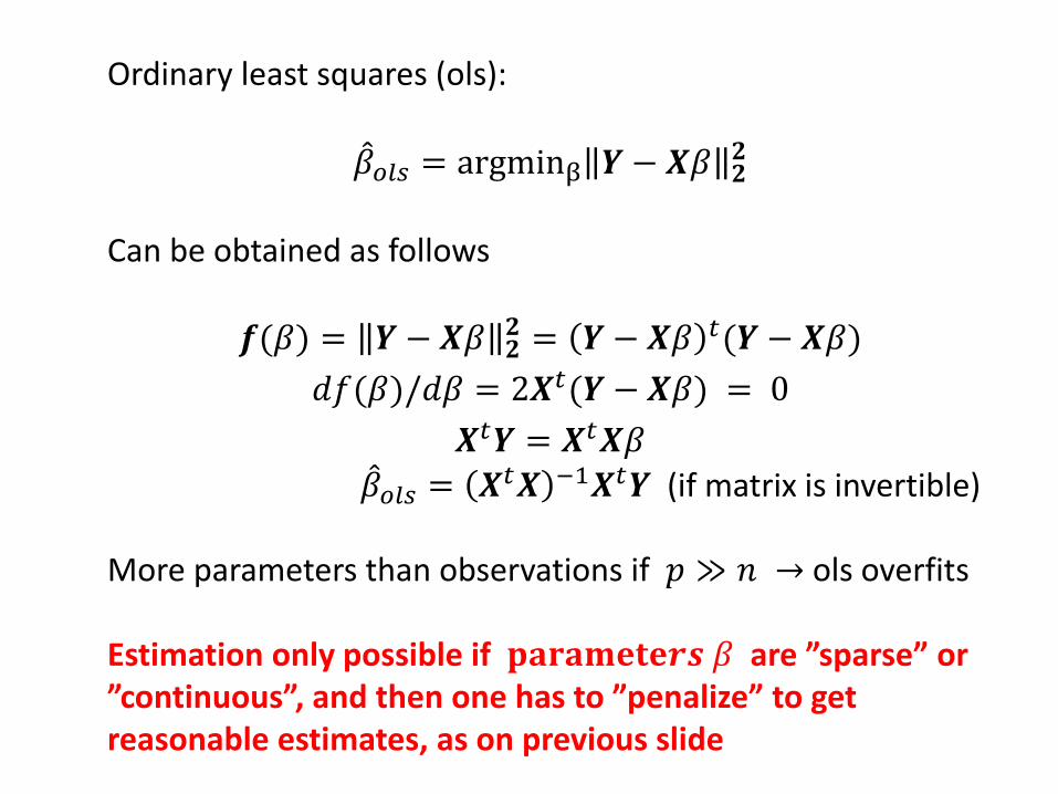
Ordinary least squares (ols):

𝛽 𝑜𝑙𝑠 = argminβ 𝒀 − 𝑿𝛽 𝟐𝟐

Can be obtained as follows

𝒇(𝛽) = 𝒀 − 𝑿𝛽 𝟐𝟐 = 𝒀 − 𝑿𝛽 𝑡(𝒀 − 𝑿𝛽)

𝑑𝑓(𝛽)/𝑑𝛽 = 2𝑿𝑡(𝒀 − 𝑿𝛽) = 0

𝑿𝑡𝒀 = 𝑿𝑡𝑿𝛽

𝛽 𝑜𝑙𝑠 = 𝑿𝑡𝑿 −1𝑿𝑡𝒀 (if matrix is invertible) More parameters than observations if 𝑝 ≫ 𝑛 → ols overfits Estimation only possible if 𝐩𝐚𝐫𝐚𝐦𝐞𝐭𝐞𝒓𝒔 𝛽 are ”sparse” or ”continuous”, and then one has to ”penalize” to get reasonable estimates, as on previous slide

Contour lines of residual sum of squares (Left) “1-ball” corresponding to the Lasso. (Right) “2-ball” corresponding to Ridge regression.

Simplest case:

𝑌1 = 𝛽1 + 𝜖1 𝑌2 = 𝛽2 + 𝜖2

∙ ∙

𝑌𝑛 = 𝛽𝑛 + 𝜖𝑛

→ 𝒀 − 𝑿𝛽 𝟐𝟐 = 𝑌𝑖 − 𝛽𝑖

2, 𝛽 1 = |𝛽𝑖|𝑛𝑖=1

𝑛𝑖=1

→ 𝒀 − 𝑿𝛽 𝟐𝟐 + 𝝀 𝛽 𝟏 = 𝑌𝑖 − 𝛽𝑖

2 + 𝜆|𝛽𝑖|𝑛𝑖=1

→ 𝛽 𝑗 = 0 if 𝑌𝑗 ≤ 𝜆/2

sign(𝑌𝑗)( 𝑌𝑗 −𝜆

2)

=: 𝑔soft,

𝜆

2

(𝑌𝑖)

B&vdG 2.3: Soft tresholding

← 𝑔𝑠𝑜𝑓𝑡,1(𝑧)

Soft tresholding: orthonormal designs

Orthonormal design if 𝑿 is 𝑛 × 𝑛 and 𝑿𝑡 𝑿 = 𝑛𝑰𝒏 Ex (designed experiment with 3 factors):

𝑌 = 𝛽1 + 𝑋2𝛽2 + 𝑋3𝛽3 + 𝑋4𝛽4 + 𝜖 𝛽1 is the mean 𝑋2 = 1 if first factor is high, 𝑋2 = −1 if first factor is low, etc

Type equation here.

𝑿 =

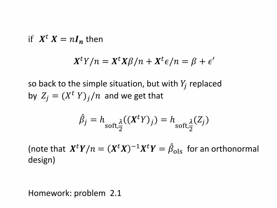
if 𝑿𝑡 𝑿 = 𝑛𝑰𝒏 then

𝑿𝑡𝑌/𝑛 = 𝑿𝑡𝑿𝛽/𝑛 + 𝑿𝑡𝜖/𝑛 = 𝛽 + 𝜖′ so back to the simple situation, but with 𝑌𝑗 replaced

by 𝑍𝑗 = (𝑋𝑡 𝑌)𝑗/𝑛 and we get that

𝛽 𝑗 = ℎsoft,

𝜆2

(𝑿𝑡𝑌 𝑗) = ℎsoft,

𝜆2

(𝑍𝑗)

(note that 𝑿𝑡𝒀/𝑛 = 𝑿𝑡𝑿 −1𝑿𝑡𝒀 = 𝛽 ols for an orthonormal design) Homework: problem 2.1

B&vdG 2.4: Prediction

is to find 𝑓 𝑥 = 𝐸 𝑌 𝑋 = 𝑥) = 𝑥(𝑗)𝛽𝑗𝑝𝑗=1 , and hence is

closely related to estimation of 𝛽. If we use the Lasso for estimation we get the estimated predictor

𝑓 𝜆 𝑥 = 𝑥𝑡 𝛽 𝜆 = 𝑥(𝑗)𝛽 𝑗(𝜆)𝑝

𝑗=1

But, how should one chose 𝜆?

HTF 7.10 , 10-fold crossvalidation

1: split (somehow) the data into 10 approximately equally sized groups 2: for each 𝑌𝑖 use the Lasso to estimate 𝛽 from the 9 groups

which do not contain 𝑌𝑖, call this estimate 𝛽 −𝑖 𝜆 , and use it to compute the predictor

𝑓 𝜆−𝑖

𝑥𝑖 = 𝑥𝑖𝑗

𝛽 𝑗(−𝑖)

(𝜆)𝑝𝑗=1

3: compute the crossvalidated mean square prediction error

𝑒 𝜆 = (𝑌𝑖 − 𝑓 𝜆−𝑖

𝑥𝑖 )2𝑛

𝑖=1

4: repeat this for a grid of 𝜆-values, choose the 𝜆 which gives the smallest 𝑒 𝜆 (note that for each 𝜆 you only have to estimate the 𝛽-s 10 times, not 𝑛 times)

B&vdG 2.4.1.1

Lymph node status of cancer patients: 𝑌 = 0 or 1

𝑛 = 49 breast cancer tumor samples 𝑝 = 7129 gene expression measurements/tumor sample Doesn’t follow model, but one can still use (crossvalidated )

Lasso to compute 𝑓 𝜆 𝑥 = 𝑥(𝑗)𝛽 𝑗(𝜆)𝑝𝑗=1 and then use it for

classification: classify status of observation with design

vector 𝑥 as 1 if 𝑓 𝜆 𝑥 > 1/2 and as 0 if 𝑓 𝜆 𝑥 ≤ 1/2.

Compared with other method, also through crossvalidation: randomly divide sample into 2/3 training data and 1/3 test data, do entire model fitting on training data, count misclassifications on test data, repeat 100 times, compute average misclassification percentages: Lasso 21% alt. 35%. Average number of non-zero 𝛽-s for Lasso was 13 .

Choice of estimation method

How does one choose between different estimation metods: Lasso, ridge regression, ols, …? • Sometimes, e.g. in signal processing, one can try out the

methods in situations where one can see how well they work (but still, it’s imposible to try all methods which have been suggested)

• Understanding

• Simulation

• Asymptotics

B&vdG 2.4.2: Asymptotics

In basic statistics asymptotics the model is fixed and 𝑛, the number of observations, tends to infinity (and one then assumes that in a practical situations with large 𝑛 distributions are well described by the asymptotic distribution). Not possible for 𝑝 ≫ 𝑛 since if the model (and thus 𝑝, the number of parameters) is kept fixed, then as 𝑛 gets large one gets that 𝑝 < 𝑛. One instead has to use triangular arrays, where 𝑝 = 𝑝𝑛 tends to infinity at the same time as n tends to infinity.

Triangular arrays

In asymptotic statments B&vdG typically assume that 𝑝 =

𝑝𝑛, 𝐗 = 𝐗n = Xn;i(j)

, and 𝛽 = 𝛽𝑛 = 𝛽𝑛;𝑗 all change as

𝑛 → ∞, typically with 𝑝𝑛 → ∞ faster than 𝑛 i.e. with 𝑝𝑛/𝑛 → ∞ as 𝑛 → ∞. Thus one considers a sequence of models

𝒀𝒏 = 𝑿𝑛𝛽𝑛 + 𝜖𝑛, or in more detail

𝑌𝑛;𝑖 = 𝑋𝑛;𝑖(𝑗)

𝛽𝑛;𝑗 + 𝜖𝑖 , for i = 1, ⋯ 𝑛,𝑝𝑛

𝑗=1

and derive asymptotic inequalities and limit distributions for such ”triangular arrays”, for 𝑛 → ∞

Prediction consistency

𝛽 𝑛 𝜆𝑛 − 𝛽𝑛0 𝑡

Σ𝑿𝑛 𝛽 𝑛 𝜆𝑛 − 𝛽𝑛0 = 𝑜𝑝 1

for Σ𝑿𝑛 = 𝑿𝑛

𝒕 𝑿𝑛/𝑛 for a fixed design, and Σ𝑿𝑛 equal to the

covariance matrix of the covariates vector 𝑋𝑛, for a random design with the covariate vectors in the different rows i.i.d. (𝑍𝑛 = 𝑜𝑝(1) means that 𝑃 𝑍𝑛 > 𝜖 → 0 as 𝑛 → ∞, for

any 𝜖 > 0, i.e. that 𝑍𝑛 tends to zero in probability) Conditions needed to obtain prediction consistency include

𝛽𝑛0

1 = 𝑜(𝑛

log 𝑝𝑛 ), 𝐾−1 log 𝑝𝑛/𝑛 < 𝜆𝑛 < 𝐾 log 𝑝𝑛/𝑛

for some constant 𝐾, and that the 𝜖𝑛;𝑖 , 𝑖 = 1, ⋯ 𝑛 are i.i.d. with finite variance.

The quantity 𝛽 𝑛 𝜆𝑛 − 𝛽𝑛0 𝑡

Σ𝑿𝑛 𝛽 𝑛 𝜆𝑛 − 𝛽𝑛0 = 𝑜𝑝 1

equals

𝑿𝑛 𝛽 𝑛(𝜆𝑛) − 𝛽𝑛0

2

2/𝑛 for a fixed design,

𝐸 (𝑋𝑛;𝑛𝑒𝑤 𝛽 𝑛 𝜆𝑛 − 𝛽𝑛0 )2 for a random design,

and where 𝑋𝑛 𝛽 𝑛 𝜆𝑛 − 𝛽𝑛0 is the difference between the

estimated and the true predictor (= regression function).

Oracle inequality

𝐸 𝑿 𝛽 𝑛(𝜆𝑛) − 𝛽𝑛0

2

2/𝑛 = (𝑋𝑖 𝛽 𝑛(𝜆𝑛) − 𝛽𝑛

0 2𝑛𝑖=1 /𝑛

= 𝑂(𝑠𝑛;0log𝑝𝑛

𝑛𝜙𝑛2 ),

where 𝑠𝑛;0 = card Sn;0 = Sn;0 is the number of

elemements in the set S0;n = 𝑗; 𝛽𝑛;𝑗0 ≠ 0, 𝑗 = 1, ⋯ 𝑝𝑛 of

active variables, and 𝜙𝑛2 is a compatablity constant

determined by the design matrix 𝑿𝑛.

means roughly that using the estimated predictor instead of the true one adds a (random) error of the size slightly larger

than 1

𝑛

Requires further conditions.

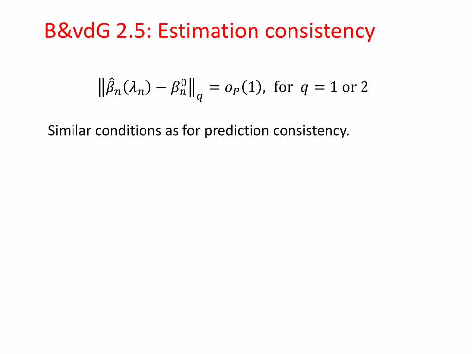
B&vdG 2.5: Estimation consistency

𝛽 𝑛 𝜆𝑛 − 𝛽𝑛0

𝑞= 𝑜𝑃 1 , for 𝑞 = 1 or 2

Similar conditions as for prediction consistency.

Variable screening

𝑆 0;𝑛(𝜆) = 𝑗; 𝛽 𝑛;𝑗(𝜆) ≠ 0, 𝑗 = 1, ⋯ 𝑝𝑛

Typically, the Lasso solutions 𝛽 𝑛0 are not unique (e.g. they are

not unique if 𝑝 > 𝑛) but still 𝑆 0;𝑛(𝜆) is unique (Lemma 2.1).

Further, 𝑆 0;𝑛 𝜆 ≤ min n, pn .

𝑆 0;𝑛relevant(𝐶)

(𝜆) = 𝑗; 𝛽 𝑛;𝑗(𝜆) ≠ 0, 𝑗 = 1, ⋯ 𝑝𝑛

is the true set of ”relevant” variables. Asymptotically, under

suitable conditions, 𝑆 0;𝑛(𝜆) will contain 𝑆0;𝑛relevant(𝐶), but

often, depending on the value of 𝜆, it will contain many more variables. For choice of 𝜆, read B&vdG 2.5.1.

Homework: Problems 2.2 and 2.3.

B&vdG 2.5.2

Motif regression for DNA binding sites: 𝑌𝑖 binding intensity of H1F1𝛼 in coarse DNA segment 𝑖

𝑋𝑖(𝑗)

abundance score of candidate motif 𝑗 in DNA segment

𝑖

𝑖 = 1, ⋯ 𝑛 = 287; 𝑗 = 1, ⋯ 𝑝 =195

𝑌𝑖 = 𝜇 + 𝑋𝑖(𝑗)

𝛽𝑗 + 𝜖𝑖 , for i = 1, ⋯ 287,195

𝑗=1

Scale covariates 𝑋 to same empirical variance, subtract 𝑌 ,

do Lasso with 𝜆 = 𝜆 CV choosen by 10-fold crossvalidation for

optimal prediction. Gives |𝑆 𝜆 CV | = 26 non-zero 𝛽 𝜆 CV

estimates. B&vdG believe these include true active variables

B&vdG 2.6: Variable selection

𝛽 𝜆 = argminβ( 𝒀 − 𝑿𝛽 𝟐𝟐/𝑛 + 𝜆 𝛽 0

0)

where 𝛽 00 = 1(𝛽𝑗 ≠ 0)

𝑝𝑗=1

Not convex: naive solution would be to go through all possible sub-models (i.e. models with some of the 𝛽-s set to 0), compute the ols for each of these models, and then chose the model which minimizes the right-hand side. However, there are 2𝑝 submodels, and if 𝑝 is not small, this isn’t feasible. More efficient algoritms exist, but still a difficult/infeasible problem if 𝑝 is not small.

One possibility is to first use (some variant of) the Lasso to select a set of variables which with high probability includes the set of active variables, and then only do the minimization of the ℓ0 penalized mean square error among these variables. Typically reduces the number of operations needed for the minimization to

𝑂 𝑛𝑝min 𝑛, 𝑝

However this requires that the Lasso in fact selects all active variables/parameters. Asymptotic conditions to ensure this include that

inf𝑗∈𝑆0

𝛽𝑗 ≫ 𝑠0log 𝑝/𝑛

and neigbourhood stability or irrepresentable condition holds

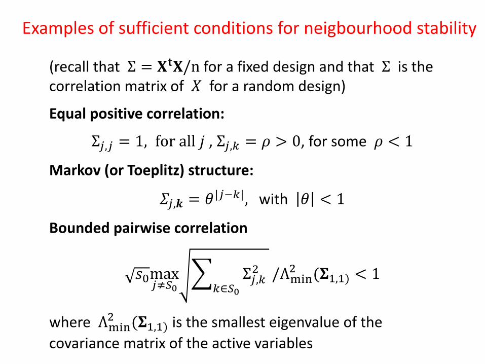
(recall that Σ = 𝐗𝐭𝐗/n for a fixed design and that Σ is the correlation matrix of 𝑋 for a random design)

Equal positive correlation:

Σ𝑗,𝑗 = 1, for all 𝑗 , Σ𝑗,𝑘 = 𝜌 > 0, for some 𝜌 < 1

Markov (or Toeplitz) structure:

𝛴𝑗,𝒌 = 𝜃|𝑗−𝑘|, with 𝜃 < 1

Bounded pairwise correlation

𝑠0max𝑗≠𝑆0

Σ𝑗,𝑘 2

𝑘∈𝑆0

/Λmin2 (𝚺1,1) < 1

where Λmin2 (𝚺1,1) is the smallest eigenvalue of the

covariance matrix of the active variables

Examples of sufficient conditions for neigbourhood stability