High Dimensional Bayesian Optimisation and Bandits via ...kkandasa/pubs/kandasamyICML15addGPUCB.pdf · High Dimensional Bayesian Optimisation and Bandits via Additive Models Kirthevasan

High Dimensional Bayesian Optimisation and Bandits via Additive Models

Kirthevasan Kandasamy [email protected] Schneider [email protected] Poczos [email protected]

Carnegie Mellon University, Pittsburgh, PA, USA

AbstractBayesian Optimisation (BO) is a technique usedin optimising a D-dimensional function whichis typically expensive to evaluate. While therehave been many successes for BO in low dimen-sions, scaling it to high dimensions has been no-toriously difficult. Existing literature on the topicare under very restrictive settings. In this paper,we identify two key challenges in this endeavour.We tackle these challenges by assuming an addi-tive structure for the function. This setting is sub-stantially more expressive and contains a richerclass of functions than previous work. We provethat, for additive functions the regret has only lin-ear dependence on D even though the functiondepends on all D dimensions. We also demon-strate several other statistical and computationalbenefits in our framework. Via synthetic exam-ples, a scientific simulation and a face detectionproblem we demonstrate that our method outper-forms naive BO on additive functions and on sev-eral examples where the function is not additive.

1. IntroductionIn many applications we are tasked with zeroth order op-timisation of an expensive to evaluate function f in D di-mensions. Some examples are hyper parameter tuning inexpensive machine learning algorithms, experiment design,optimising control strategies in complex systems, and sci-entific simulation based studies. In such applications, f isa blackbox which we can interact with only by queryingfor the value at a specific point. Related to optimisation isthe bandits problem arising in applications such as onlineadvertising and reinforcement learning. Here the objectiveis to maximise the cumulative sum of all queries. In eithercase, we need to find the optimum of f using as few queriesas possible by managing exploration and exploitation.

Proceedings of the 32nd International Conference on MachineLearning, Lille, France, 2015. JMLR: W&CP volume 37. Copy-right 2015 by the author(s).

Bayesian Optimisation (Mockus & Mockus, 1991) refersto a suite of methods that tackle this problem by modelingf as a Gaussian Process (GP). In such methods, the chal-lenge is two fold. At time step t, first estimate the unknownf from the query value-pairs. Then use it to intelligentlyquery at xt where the function is likely to be high. Forthis, we first use the posterior GP to construct an acquisi-tion function ϕt which captures the value of the experimentat a point. Then we maximise ϕt to determine xt.

Gaussian process bandits and Bayesian optimisation (GPB/BO) have been successfully applied in many applicationssuch as tuning hyperparameters in learning algorithms(Snoek et al., 2012; Bergstra et al., 2011; Mahendran et al.,2012), robotics (Lizotte et al., 2007; Martinez-Cantin et al.,2007) and object tracking (Denil et al., 2012). However,all such successes have been in low (typically < 10) di-mensions (Wang et al., 2013). Expensive high dimensionalfunctions occur in several problems in fields such as com-puter vision (Yamins et al., 2013), antenna design (Hornbyet al., 2006), computational astrophysics (Parkinson et al.,2006) and biology (Gonzalez et al., 2014). Scaling GPB/BO methods to high dimensions for practical problems hasbeen challenging. Even current theoretical results suggestthat GPB/ BO is exponentially difficult in high dimensionswithout further assumptions (Srinivas et al., 2010; Bull,2011). To our knowledge, the only approach to date hasbeen to perform regular GPB/ BO on a low dimensionalsubspace. This works only under strong assumptions.

We identify two key challenges in scaling GPB/ BO to highdimensions. The first is the statistical challenge in esti-mating the function. Nonparametric regression is inher-ently difficult in high dimensions with known lower boundsdepending exponentially in dimension (Gyorfi et al., 2002).The often exponential sample complexity for regression isinvariably reflected in the regret bounds for GPB/ BO. Thesecond is the computational challenge in maximisingϕt. Commonly used global optimisation heuristics usedto maximise ϕt themselves require computation exponen-tial in dimension. Any attempt to scale GPB/ BO to highdimensions must effectively address these two concerns.

Additive Gaussian Process Optimisation and Bandits

In this work, we embark on this challenge by treating fas an additive function of mutually exclusive lower dimen-sional components. Our contributions in this work are:

1. We present the Add-GP-UCB algorithm for optimi-sation and bandits of an additive function. An attrac-tive property is that we use an acquisition functionwhich is easy to optimise in high dimensions.

2. In our theoretical analysis we bound the regret forAdd-GP-UCB. We show that it has only linear de-pendence on the dimension D when f is additive1.

3. Empirically we demonstrate that Add-GP-UCB out-performs naive BO on synthetic experiments, an astro-physical simulator and the Viola and Jones face detec-tion problem. Furthermore Add-GP-UCB does wellon several examples when the function is not additive.

A Matlab implementation of our methods is available on-line at github.com/kirthevasank/add-gp-bandits.

2. Related WorkGPB/ BO methods follow a family of GP based activelearning methods which select the next experiment basedon the posterior (Osborne et al., 2012; Ma et al., 2015;Kandasamy et al., 2015). In the GPB/ BO setting, com-mon acquisition functions include Expected improvement(Mockus, 1994), probability of improvement (Jones et al.,1998), Thompson sampling (Thompson, 1933) and upperconfidence bound (Auer, 2003). Of particular interest tous, is the Gaussian process upper confidence bound (GP-UCB). It was first proposed and analysed in the noisy set-ting by Srinivas et al. (2010) and extended to the noiselesscase by de Freitas et al. (2012). Some literature stud-ies variants, such as combining several acquisition func-tions (Hoffman et al., 2011) and querying in batches (Az-imi et al., 2010).

To our knowledge, most literature for GPB/ BO in highdimensions are in the setting where the function variesonly along a very low dimensional subspace (Chen et al.,2012; Wang et al., 2013; Djolonga et al., 2013). In theseworks, the authors do not encounter either challenge asthey perform GPB/ BO in either a random or carefully se-lected lower dimensional subspace. However, assumingthat the problem is an easy (low dimensional) one hidingin a high dimensional space is often too restrictive. In-deed, our experimental results confirm that such methodsperform poorly on real applications when the assumptionsare not met. While our additive assumption is strong in itsown right, it is considerably more expressive. It is more

1Post-publication it was pointed out to us that there was a bugin our analysis. We are working on resolving it and will post anupdate shortly. See Section 6 for more details.

general than the setting in Chen et al. (2012). Even thoughit does not contain the settings in Djolonga et al. (2013);Wang et al. (2013), unlike them, we still allow the functionto vary along the entire domain.

Using an additive structure is standard in high dimensionalregression literature both in the GP framework and other-wise. Hastie & Tibshirani (1990); Ravikumar et al. (2009)treat the function as a sum of one dimensional components.Our additive framework is more general. Duvenaud et al.(2011) assume a sum of functions of all combinations oflower dimensional coordinates. These literature argue thatusing an additive model has several advantages even if f isnot additive. It is a well understood notion in statistics thatwhen we only have a few samples, using a simpler modelto fit our data may give us a better trade off for estimationerror against approximation error. This observation is cru-cial: in many applications for Bayesian optimisation we areforced to work in the low sample regime since calls to theblackbox are expensive. Though the additive assumptionis biased for nonadditive functions, it enables us to do wellwith only a few samples. While we have developed theo-retical results only for additive f , empirically we show thatour additive model outperforms naive GPB/ BO even whenthe underlying function is not additive.

Analyses of GPB/ BO methods focus on the query com-plexity of f which is the dominating cost in relevant appli-cations. It is usually assumed that ϕt can be maximised toarbitrary precision at negligible cost. Common techniquesto maximise ϕt include grid search, Monte Carlo and mul-tistart methods (Brochu et al., 2010). In our work we usethe Dividing Rectangles (DiRect) algorithm of Jones et al.(1993). While these methods are efficient in low dimen-sions they require exponential computation in high dimen-sions. It is widely acknowledged in the community thatthis is a critical bottleneck in scaling GPB/ BO to high di-mensions (de Freitas, 2014). While we still work in theparadigm where evaluating f is expensive and characteriseour theoretical results in terms of query complexity, we be-lieve that assuming arbitrary computational power to opti-mise ϕt is too restrictive. For instance, in hyperparametertuning the budget for determining the next experiment isdictated by the cost of the learning algorithm. In online ad-vertising and robotic reinforcement learning we need to actin under a few seconds or real time.

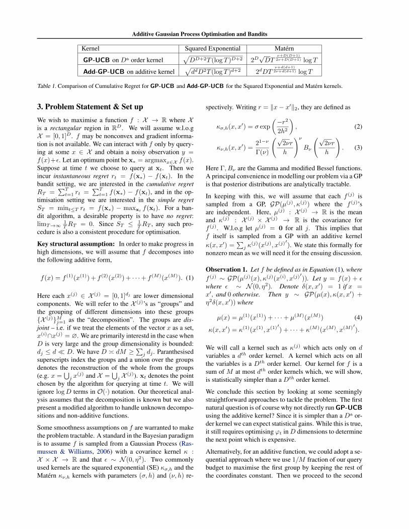
In this manuscript, Section 3 formally details our problemand assumptions. We present Add-GP-UCB in Section 4and our theoretical results in Section 4.3. All proofs are de-ferred to Appendix B. We summarize the regrets for Add-GP-UCB and GP-UCB in Table 1. In Section 5 wepresent the experiments.


Kernel Squared Exponential Matern

GP-UCB on Dth order kernel√DD+2T (log T )D+2 2D

√DT

ν+D(D+1)2ν+D(D+1) log T

Add-GP-UCB on additive kernel√ddD2T (log T )d+2 2dDT

ν+d(d+1)2ν+d(d+1) log T

Table 1. Comparison of Cumulative Regret for GP-UCB and Add-GP-UCB for the Squared Exponential and Matern kernels.

3. Problem Statement & Set upWe wish to maximise a function f : X → R where Xis a rectangular region in RD. We will assume w.l.o.gX = [0, 1]D. f may be nonconvex and gradient informa-tion is not available. We can interact with f only by query-ing at some x ∈ X and obtain a noisy observation y =f(x)+ε. Let an optimum point be x∗ = argmaxx∈X f(x).Suppose at time t we choose to query at xt. Then weincur instantaneous regret rt = f(x∗) − f(xt). In thebandit setting, we are interested in the cumulative regretRT =

∑Tt=1 rt =

∑Tt=1 f(x∗) − f(xt), and in the op-

timisation setting we are interested in the simple regretST = mint≤T rt = f(x∗) − maxxt f(xt). For a ban-dit algorithm, a desirable property is to have no regret:limT→∞

1TRT = 0. Since ST ≤ 1

TRT , any such pro-cedure is also a consistent procedure for optimisation.

Key structural assumption: In order to make progress inhigh dimensions, we will assume that f decomposes intothe following additive form,

f(x) = f (1)(x(1)) + f (2)(x(2)) + · · ·+ f (M)(x(M)). (1)

Here each x(j) ∈ X (j) = [0, 1]dj are lower dimensionalcomponents. We will refer to the X (j)’s as “groups” andthe grouping of different dimensions into these groupsX (j)Mj=1 as the “decomposition”. The groups are dis-joint – i.e. if we treat the elements of the vector x as a set,x(i)∩x(j) = ∅. We are primarily interestd in the case whenD is very large and the group dimensionality is bounded:dj ≤ d D. We have D dM ≥

∑j dj . Paranthesised

superscripts index the groups and a union over the groupsdenotes the reconstruction of the whole from the groups(e.g. x =

⋃j x

(j) and X =⋃j X (j)). xt denotes the point

chosen by the algorithm for querying at time t. We willignore logD terms in O(·) notation. Our theoretical anal-ysis assumes that the decomposition is known but we alsopresent a modified algorithm to handle unknown decompo-sitions and non-additive functions.

Some smoothness assumptions on f are warranted to makethe problem tractable. A standard in the Bayesian paradigmis to assume f is sampled from a Gaussian Process (Ras-mussen & Williams, 2006) with a covarince kernel κ :X × X → R and that ε ∼ N (0, η2). Two commonlyused kernels are the squared exponential (SE) κσ,h and theMatern κν,h kernels with parameters (σ, h) and (ν, h) re-

spectively. Writing r = ‖x− x′‖2, they are defined as

κσ,h(x, x′) = σ exp

(−r2

2h2

), (2)

κν,h(x, x′) =21−ν

Γ(ν)

(√2νr

h

)νBν

(√2νr

h

). (3)

Here Γ, Bν are the Gamma and modified Bessel functions.A principal convenience in modelling our problem via a GPis that posterior distributions are analytically tractable.

In keeping with this, we will assume that each f (j) issampled from a GP, GP(µ(j), κ(j)) where the f (j)’sare independent. Here, µ(j) : X (j) → R is the meanand κ(j) : X (j) × X (j) → R is the covariance forf (j). W.l.o.g let µ(j) = 0 for all j. This implies thatf itself is sampled from a GP with an additive kernelκ(x, x′) =

∑j κ

(j)(x(j), x(j)′). We state this formally fornonzero mean as we will need it for the ensuing discussion.

Observation 1. Let f be defined as in Equation (1), wheref (j) ∼ GP(µ(j)(x), κ(j)(x(i), x(j)′)). Let y = f(x) + εwhere ε ∼ N (0, η2). Denote δ(x, x′) = 1 if x =x′, and 0 otherwise. Then y ∼ GP(µ(x), κ(x, x′) +η2δ(x, x′)) where

µ(x) = µ(1)(x(1)) + · · ·+ µ(M)(x(M)) (4)

κ(x, x′) = κ(1)(x(1), x(1)′) + · · ·+ κ(M)(x(M), x(M)′).

We will call a kernel such as κ(j) which acts only on dvariables a dth order kernel. A kernel which acts on allthe variables is a Dth order kernel. Our kernel for f is asum of M at most dth order kernels which, we will show,is statistically simpler than a Dth order kernel.

We conclude this section by looking at some seeminglystraightforward approaches to tackle the problem. The firstnatural question is of course why not directly run GP-UCBusing the additive kernel? Since it is simpler than a Dth or-der kernel we can expect statistical gains. While this is true,it still requires optimising ϕt inD dimensions to determinethe next point which is expensive.

Alternatively, for an additive function, we could adopt a se-quential approach where we use 1/M fraction of our querybudget to maximise the first group by keeping the rest ofthe coordinates constant. Then we proceed to the second


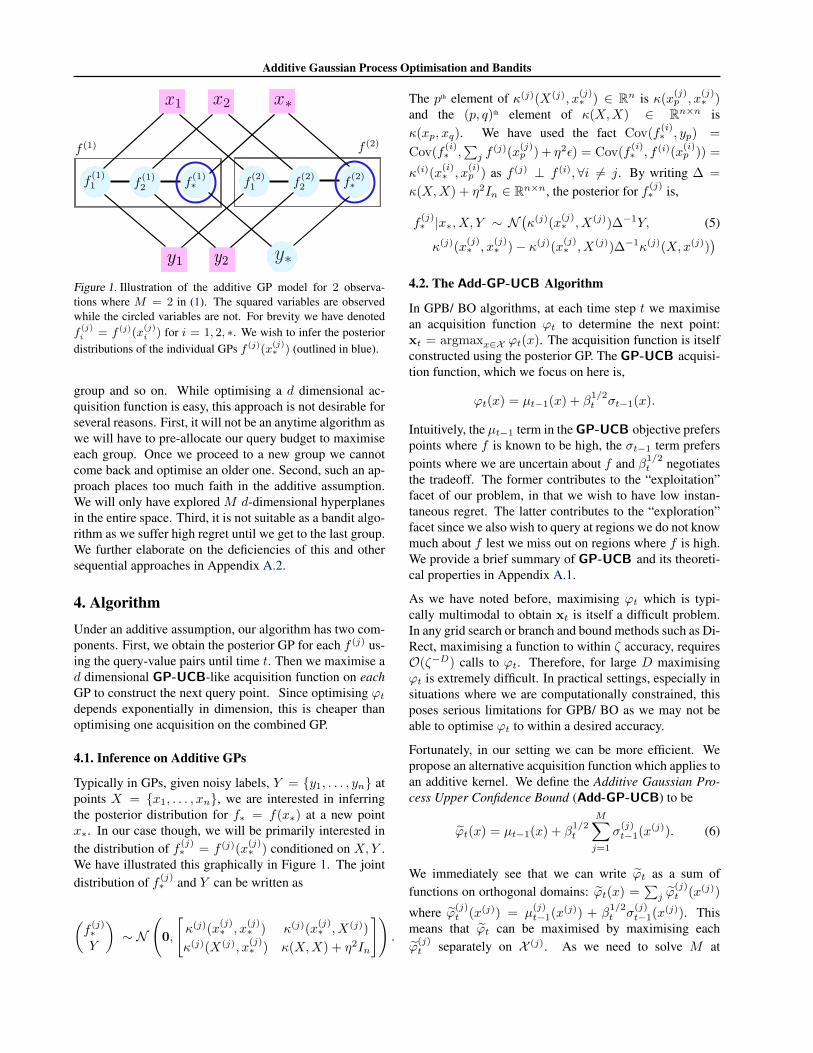
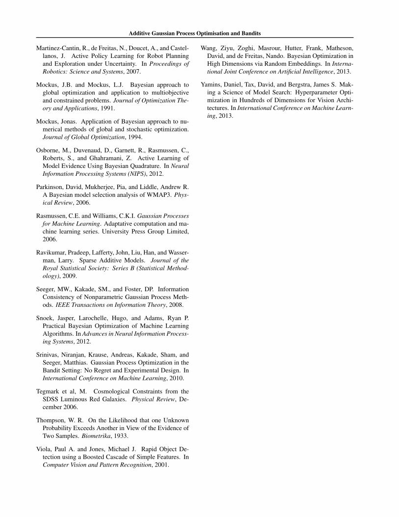
Figure 1. Illustration of the additive GP model for 2 observa-tions where M = 2 in (1). The squared variables are observedwhile the circled variables are not. For brevity we have denotedf(j)i = f (j)(x

(j)i ) for i = 1, 2, ∗. We wish to infer the posterior

distributions of the individual GPs f (j)(x(j)∗ ) (outlined in blue).

group and so on. While optimising a d dimensional ac-quisition function is easy, this approach is not desirable forseveral reasons. First, it will not be an anytime algorithm aswe will have to pre-allocate our query budget to maximiseeach group. Once we proceed to a new group we cannotcome back and optimise an older one. Second, such an ap-proach places too much faith in the additive assumption.We will only have explored M d-dimensional hyperplanesin the entire space. Third, it is not suitable as a bandit algo-rithm as we suffer high regret until we get to the last group.We further elaborate on the deficiencies of this and othersequential approaches in Appendix A.2.

4. AlgorithmUnder an additive assumption, our algorithm has two com-ponents. First, we obtain the posterior GP for each f (j) us-ing the query-value pairs until time t. Then we maximise ad dimensional GP-UCB-like acquisition function on eachGP to construct the next query point. Since optimising ϕtdepends exponentially in dimension, this is cheaper thanoptimising one acquisition on the combined GP.

4.1. Inference on Additive GPs

Typically in GPs, given noisy labels, Y = y1, . . . , yn atpoints X = x1, . . . , xn, we are interested in inferringthe posterior distribution for f∗ = f(x∗) at a new pointx∗. In our case though, we will be primarily interested inthe distribution of f (j)

∗ = f (j)(x(j)∗ ) conditioned on X,Y .

We have illustrated this graphically in Figure 1. The jointdistribution of f (j)

∗ and Y can be written as

(f

(j)∗Y

)∼ N

(0,

[κ(j)(x

(j)∗ , x

(j)∗ ) κ(j)(x

(j)∗ , X(j))

κ(j)(X(j), x(j)∗ ) κ(X,X) + η2In

]).

The pth element of κ(j)(X(j), x(j)∗ ) ∈ Rn is κ(x

(j)p , x

(j)∗ )

and the (p, q)th element of κ(X,X) ∈ Rn×n isκ(xp, xq). We have used the fact Cov(f

(i)∗ , yp) =

Cov(f(i)∗ ,∑j f

(j)(x(j)p ) + η2ε) = Cov(f

(i)∗ , f (i)(x

(i)p )) =

κ(i)(x(i)∗ , x

(i)p ) as f (j) ⊥ f (i),∀i 6= j. By writing ∆ =

κ(X,X) + η2In ∈ Rn×n, the posterior for f (j)∗ is,

f(j)∗ |x∗, X, Y ∼ N

(κ(j)(x

(j)∗ , X(j))∆−1Y, (5)

κ(j)(x(j)∗ , x

(j)∗ )− κ(j)(x

(j)∗ , X(j))∆−1κ(j)(X,x(j))

)4.2. The Add-GP-UCB Algorithm

In GPB/ BO algorithms, at each time step t we maximisean acquisition function ϕt to determine the next point:xt = argmaxx∈X ϕt(x). The acquisition function is itselfconstructed using the posterior GP. The GP-UCB acquisi-tion function, which we focus on here is,

ϕt(x) = µt−1(x) + β1/2t σt−1(x).

Intuitively, the µt−1 term in the GP-UCB objective preferspoints where f is known to be high, the σt−1 term preferspoints where we are uncertain about f and β1/2

t negotiatesthe tradeoff. The former contributes to the “exploitation”facet of our problem, in that we wish to have low instan-taneous regret. The latter contributes to the “exploration”facet since we also wish to query at regions we do not knowmuch about f lest we miss out on regions where f is high.We provide a brief summary of GP-UCB and its theoreti-cal properties in Appendix A.1.

As we have noted before, maximising ϕt which is typi-cally multimodal to obtain xt is itself a difficult problem.In any grid search or branch and bound methods such as Di-Rect, maximising a function to within ζ accuracy, requiresO(ζ−D) calls to ϕt. Therefore, for large D maximisingϕt is extremely difficult. In practical settings, especially insituations where we are computationally constrained, thisposes serious limitations for GPB/ BO as we may not beable to optimise ϕt to within a desired accuracy.

Fortunately, in our setting we can be more efficient. Wepropose an alternative acquisition function which applies toan additive kernel. We define the Additive Gaussian Pro-cess Upper Confidence Bound (Add-GP-UCB) to be

ϕt(x) = µt−1(x) + β1/2t

M∑j=1

σ(j)t−1(x(j)). (6)

We immediately see that we can write ϕt as a sum offunctions on orthogonal domains: ϕt(x) =

∑j ϕ

(j)t (x(j))

where ϕ(j)t (x(j)) = µ

(j)t−1(x(j)) + β

1/2t σ

(j)t−1(x(j)). This

means that ϕt can be maximised by maximising eachϕ

(j)t separately on X (j). As we need to solve M at


most d dimensional optimisation problems, it requires onlyO(Md+1ζ−d) calls to the utility function in total – far morefavourable than maximising ϕt.

Since the cost for maximising the acquisition function is akey theme in this paper let us delve into this a bit more. Onecall to ϕt requires O(Dt2) effort. For ϕt we need M callseach requiring O(djt

2) effort. So both ϕt and ϕt requirethe same effort in this front. For ϕt, we need to know theposterior for only f whereas for ϕt we need to know theposterior for each f (j). However, the brunt of the work inobtaining the posterior is the O(t3) effort in inverting thet×tmatrix ∆ in (5) which needs to be done for both ϕt andϕt. For ϕt, we can obtain the inverse once and reuse it Mtimes, so the cost of obtaining the posterior isO(t3+Mt2).Since the number of queries needed will be super linear inD and hence M , the t3 term dominates. Therefore obtain-ing each posterior f (j) is only marginally more work thanobtaining the posterior for f . Any difference here is easilyoffset by the cost for maximising the acquisition function.

The question remains then if maximising ϕt would result inlow regret. Since ϕt and ϕt are neither equivalent nor havethe same maximiser it is not immediately apparent that thisshould work. Nonetheless, intuitively this seems like a rea-sonable scheme since the

∑j σ

(j)t−1 term captures some no-

tion of the uncertainty and contributes to exploration. InTheorem 5 we show that this intuition is reasonable – max-imising ϕt achieves the same rates as ϕt for cumulative andsimple regrets if the kernel is additive.

We summarise the resulting algorithm in Algorithm 1. Inbrief, at time step t, we obtain the posterior distribution forf (j) and maximise ϕ(j)

t to determine the coordinates x(j)t .

We do this for each j and then combine them to obtain xt.

Algorithm 1 Add-GP-UCBInput: Kernels κ(1), . . . , κ(M), Decomposition (X (j))Mj=1

• D0 ← ∅,• for j = 1, . . . ,M , (µ

(j)0 , κ

(j)0 )← (0, κ(j)).

• for t = 1, 2, . . .

1. for j = 1, . . . ,M ,x

(j)t ← argmaxz∈X (j) µ

(j)t−1(z) +

√βtσ

(j)t−1(z)

2. xt ←⋃Mj=1 x

(j)t .

3. yt ← Query f at xt.4. Dt = Dt−1 ∪ (xt,yt).5. Perform Bayesian posterior updates conditioned

on Dt to obtain µ(j)t , σ

(j)t for j = 1, . . . ,M .

4.3. Main Theoretical Results

Now, we present our main theoretical contributions. Webound the regret for Add-GP-UCB under different ker-nels. Following Srinivas et al. (2010), we first bound the

statistical difficulty of the problem as determined by thekernel. We show that under additive kernels the problemis much easier than when using a full Dth order kernel.Next, we show that the Add-GP-UCB algorithm is able toexploit the additive structure and obtain the same rates asGP-UCB. The advantage to using Add-GP-UCB is thatit is much easier to optimise the acquisition function. Forour analysis, we will need Assumption 2 and Definition 3.

Assumption 2. Let f be sampled from a GP with kernel κ.κ(·, x) is L-Lipschitz for all x. Further, the partial deriva-tives of f satisfies the following high probability bound.There exists constants a, b > 0 such that,

P(

supx

∣∣∣∂f(x)

∂xi

∣∣∣ > J

)≤ ae−(J/b)2 .

The Lipschitzian condition is fairly mild and the lattercondition holds for four times differentiable stationarykernels such as the SE and Matern kernels for ν > 2(Ghosal & Roy, 2006). Srinivas et al. (2010) showedthat the statistical difficulty of GPB/ BO is determinedby the Maximum Information Gain as defined below. Webound this quantity for additive SE and Matern kernels inTheorem 4. This is our first main theorem.

Definition 3. (Maximum Information Gain) Let f ∼GP(µ, κ), yi = f(xi) + ε where ε ∼ N (0, η2). LetA = x1, . . . , xT ⊂ X be a finite subset, fA denote thefunction values at these points and yA denote the noisy ob-servations. Let I be the Shannon Mutual Information. TheMaximum Information Gain between yA and fA is

γT = maxA⊂X ,|A|=T

I(yA; fA).

Theorem 4. Assume that the kernel κ has the additive formof (4), and that each κ(j) satisfies Assumption 2. W.l.o.gassume κ(x, x′) = 1. Then,

1. If each κ(j) is a dthj order squared exponential ker-nel (2) where dj ≤ d, then γT ∈ O(Ddd(log T )d+1).

2. If each κ(j) is a dthj order Matern kernel (3)where dj ≤ d and ν > 2, then γT ∈O(D2dT

d(d+1)2ν+d(d+1) log(T )).

We use bounds on the eigenvalues of the SE and Maternkernels from Seeger et al. (2008) and a result from Srini-vas et al. (2010) which bounds the information gain via theeigendecay of the kernel. We bound the eigendecay of thesum κ via M and the eigendecay of a single κ(j). Thecomplete proof is given in Appendix B.1. The importantobservation is that the dependence on D is linear for anadditive kernel. In contrast, for a Dth order kernel this isexponential (Srinivas et al., 2010).


Next, we present our second main theorem which boundsthe regret for Add-GP-UCB for an additive kernel asgiven in Equation 4.

Theorem 5. Suppose f is constructed by sampling f (j) ∼GP(0, κ(j)) for j = 1, . . . ,M and then adding them. Letall kernels κ(j) satisfy assumption 2 for some L, a, b. Fur-ther, we maximise the acquisition function ϕt to withinζ0t−1/2 accuracy at time step t. Pick δ ∈ (0, 1) and choose

βt = 2 log

(Mπ2t2

2δ

)+ 2d log

(Dt3

)∈ O (d log t) .

Then, Add-GP-UCB attains cumulative regret RT ∈O(√

DγTT log T)

and hence simple regret ST ∈

O(√

DγT log T/T)

. Precisely, with probability > 1− δ,

∀T ≥ 1, RT ≤√

8C1βTMTγt + 2ζ0√T + C2.

where C1 = 1/ log(1 + η−2) and C2 is a constant depend-ing on a, b, D, δ, L and η.

Part of our proof uses ideas from Srinivas et al. (2010).We show that

∑j βtσ

(j)t−1(·) forms a credible interval for

f(·) about the posterior mean µt(·) for an additive kernel inAdd-GP-UCB. We relate the regret to this confidence setusing a covering argument. We also show that our regretdoesn’t suffer severely if we only approximately optimisethe acquisition provided that the accuracy improves at rateO(t−1/2). For this we establish smoothness of the poste-rior mean. The correctness of the algorithm follows fromthe fact that Add-GP-UCB can be maximised by individ-ually maximising ϕ(j)

t on each X (j). The complete proofis given in Appendix B.2. When we combine the resultsin Theorems 4 and 5 we obtain the rates given in Table 12.

One could consider alternative lower order kernels – onecandidate is the sum of all possible dth order kernels (Du-venaud et al., 2011). Such a kernel would arguably al-low us to represent a larger class of functions than ourkernel in (4). If, for instance, we choose each of themto be a SE kernel, then it can be shown that γT ∈O(Dddd+1(log T )d+1). Even though this is worse than ourkernel in poly(D) factors, it is still substantially better thanusing a Dth order kernel. However, maximising the corre-sponding utility function, either of the form ϕt or ϕt, is stilla D dimensional problem. We reiterate that what rendersour algorithm attractive in large D is not just the statisticalgains due to the simpler kernel. It is also the fact that ouracquisition function can be efficiently maximised.

4.4. Practical Considerations

Our practical implementation differs from our theoreticalanalysis in the following aspects.

2See Footnote 1.

Choice of βt: βt as specified by Theorems 5, usually tendsto be conservative in practice (Srinivas et al., 2010). Forgood empirical performance a more aggressive strategy isrequired. In our experiments, we set βt = 0.2d log(2t)which offered a good tradeoff between exploration and ex-ploitation. Note that this captures the correct dependenceon D, d and t in Theorems 5 and 6.

Data dependent prior: Our analysis assumes that weknow the GP kernel of the prior. In reality this is rarely thecase. In our experiments, we choose the hyperparametersof the kernel by maximising the GP marginal likelihood(Rasmussen & Williams, 2006) every Ncyc iterations.

Initialisation: Marginal likelihood based kernel tuningcan be unreliable with few data points. This is a problem inthe first few iterations. Following the recommendations inBull (2011) we initialise Add-GP-UCB (and GP-UCB)using Ninit points selected uniformly at random.

Decomposition & Non-additive functions: If f is ad-ditive and the decomposition is known, we use it directly.But it may not always be known or f may not be addi-tive. Then, we could treat the decomposition as a hyperpa-rameter of the additive kernel and maximise the marginallikelihood w.r.t the decomposition. However, given thatthere are D!/d!MM ! possible decompositions, comput-ing the marginal likelihood for all of them is infeasible.We circumvent this issue by randomly selecting a few(O(D)) decompositions and choosing the one with thelargest marginal likelihood. Intuitively, if the function isnot additive, with such a “partial maximisation” we canhope to capture some existing marginal structure in f . Atthe same time, even an exhaustive maximisation will not domuch better than a partial maximisation if there is no addi-tive structure. Empirically, we found that partially optimis-ing for the decomposition performed slightly better thanusing a fixed decomposition or a random decompositionat each step. We incorporate this procedure for finding anappropriate decomposition as part of the kernel hyper pa-rameter learning procedure every Ncyc iterations.

How do we choose (d,M) when f is not additive? If d islarge we allow for richer class of functions, but risk highvariance. For small d, the kernel is too simple and we havehigh bias but low variance – further optimising ϕt is easier.In practice we found that our procedure was fairly robustfor reasonable choices of d. Yet this is an interesting theo-retical question. We also believe it is a difficult one. Usingthe marginal likelihood alone will not work as the optimalchoice of d also depends on the computational budget foroptimising ϕt. We hope to study this question in futurework. For now, we give some recommendations at the end.Our modified algorithm with these practical considerationsis given below. Observe that in this specification if we used = D we have the original GP-UCB algorithm.


Algorithm 2 Practical-Add-GP-UCBInput: Ninit, Ncyc, d, M• D0 ← Ninit points chosen uniformly at random.• for t = 1, 2, . . .

1. if (t mod Ncyc = 0), Learn the kernel hyperparameters and the decomposition Xj by max-imising the GP marginal likelihood.

2. Perform steps 1-3 in Algorithm 1 with βt =0.2d log 2t.

3. Dt = Dt−1 ∪ (xt,yt).4. Perform Bayesian posterior updates conditioned

on Dt to obtain µ(j)t , σ

(j)t for j = 1, . . . ,M .

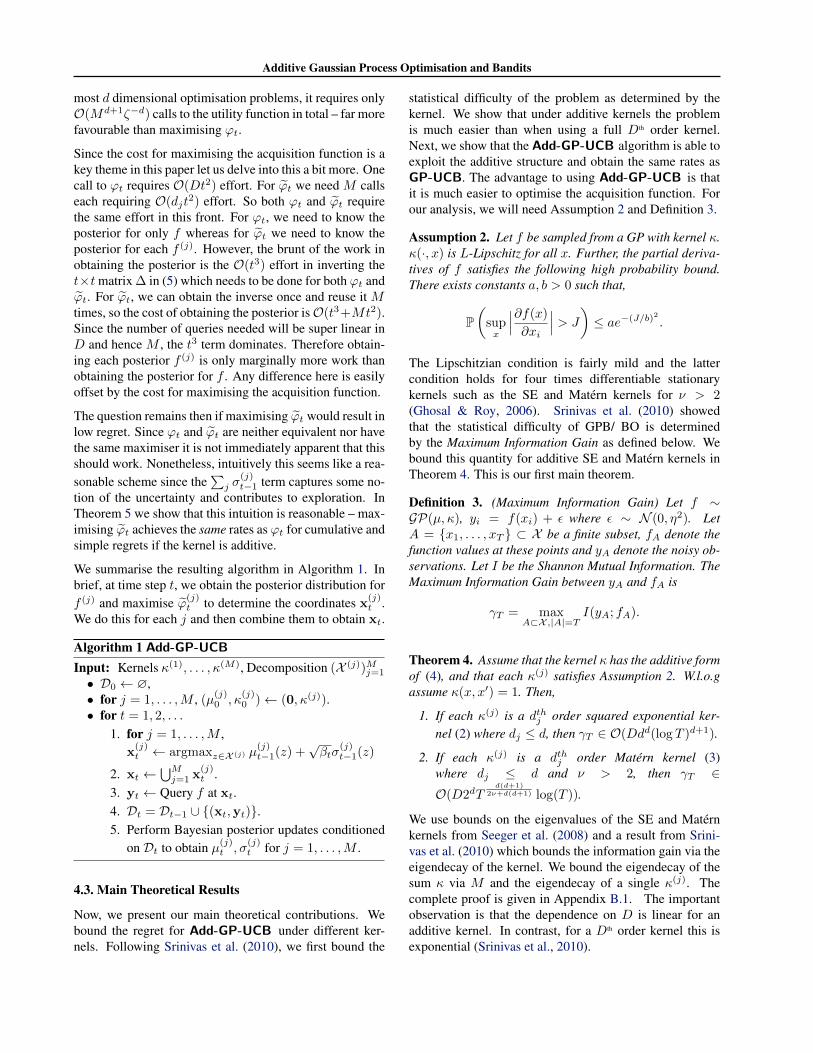
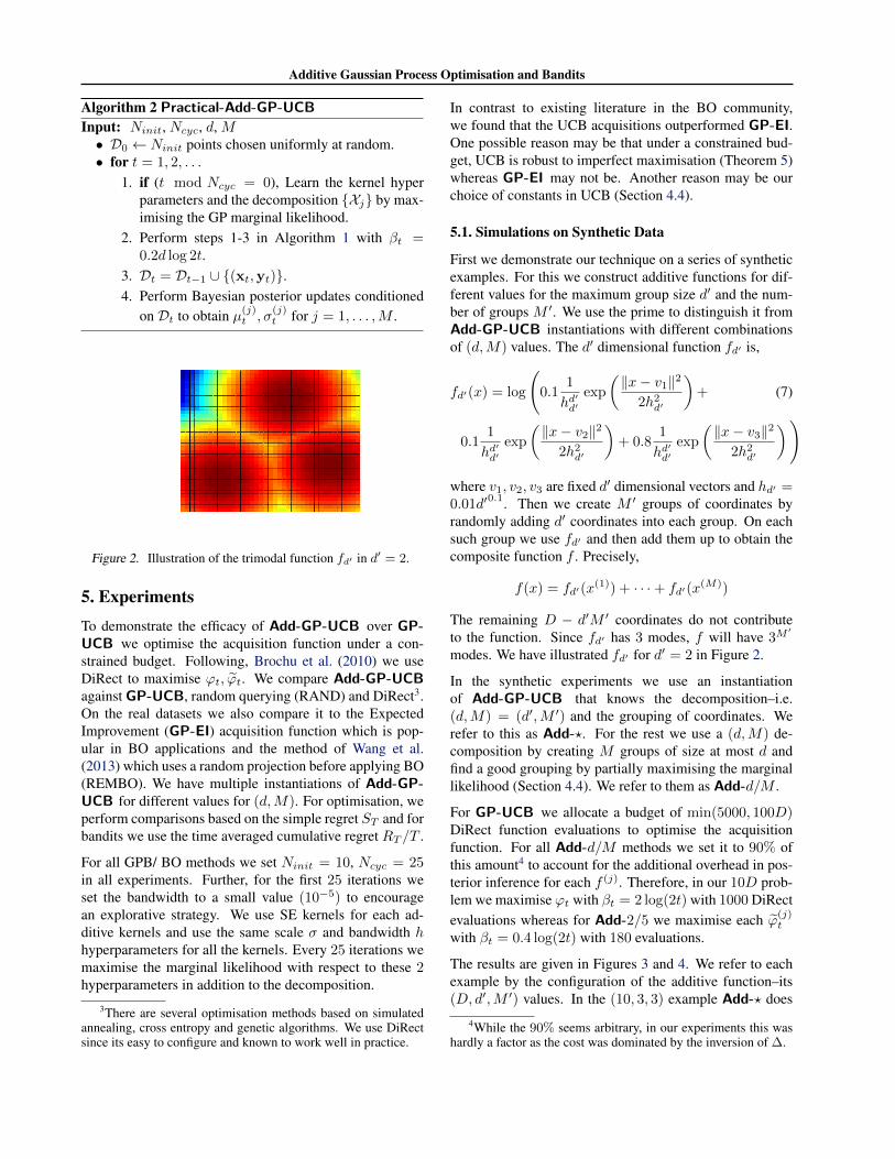
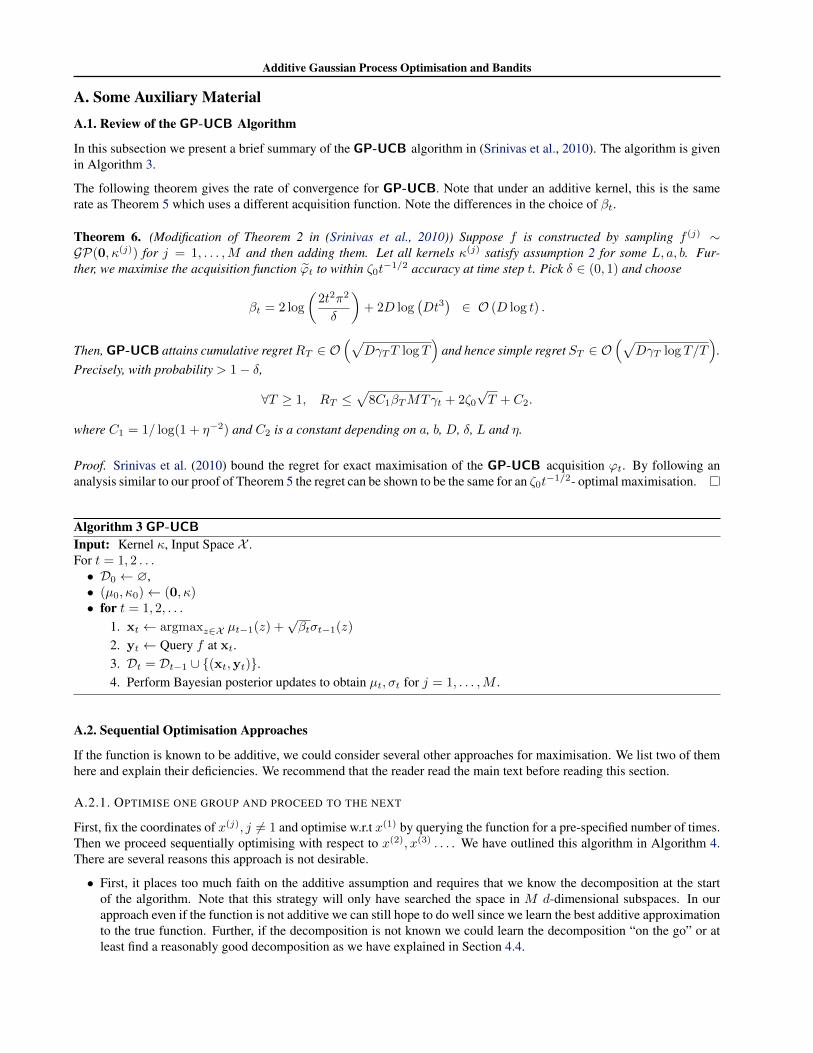
Figure 2. Illustration of the trimodal function fd′ in d′ = 2.

5. ExperimentsTo demonstrate the efficacy of Add-GP-UCB over GP-UCB we optimise the acquisition function under a con-strained budget. Following, Brochu et al. (2010) we useDiRect to maximise ϕt, ϕt. We compare Add-GP-UCBagainst GP-UCB, random querying (RAND) and DiRect3.On the real datasets we also compare it to the ExpectedImprovement (GP-EI) acquisition function which is pop-ular in BO applications and the method of Wang et al.(2013) which uses a random projection before applying BO(REMBO). We have multiple instantiations of Add-GP-UCB for different values for (d,M). For optimisation, weperform comparisons based on the simple regret ST and forbandits we use the time averaged cumulative regret RT /T .

For all GPB/ BO methods we set Ninit = 10, Ncyc = 25in all experiments. Further, for the first 25 iterations weset the bandwidth to a small value (10−5) to encouragean explorative strategy. We use SE kernels for each ad-ditive kernels and use the same scale σ and bandwidth hhyperparameters for all the kernels. Every 25 iterations wemaximise the marginal likelihood with respect to these 2hyperparameters in addition to the decomposition.

3There are several optimisation methods based on simulatedannealing, cross entropy and genetic algorithms. We use DiRectsince its easy to configure and known to work well in practice.

In contrast to existing literature in the BO community,we found that the UCB acquisitions outperformed GP-EI.One possible reason may be that under a constrained bud-get, UCB is robust to imperfect maximisation (Theorem 5)whereas GP-EI may not be. Another reason may be ourchoice of constants in UCB (Section 4.4).

5.1. Simulations on Synthetic Data

First we demonstrate our technique on a series of syntheticexamples. For this we construct additive functions for dif-ferent values for the maximum group size d′ and the num-ber of groups M ′. We use the prime to distinguish it fromAdd-GP-UCB instantiations with different combinationsof (d,M) values. The d′ dimensional function fd′ is,

fd′(x) = log

(0.1

1

hd′d′

exp

(‖x− v1‖2

2h2d′

)+ (7)

0.11

hd′d′

exp

(‖x− v2‖2

2h2d′

)+ 0.8

1

hd′d′

exp

(‖x− v3‖2

2h2d′

))

where v1, v2, v3 are fixed d′ dimensional vectors and hd′ =0.01d′

0.1. Then we create M ′ groups of coordinates byrandomly adding d′ coordinates into each group. On eachsuch group we use fd′ and then add them up to obtain thecomposite function f . Precisely,

f(x) = fd′(x(1)) + · · ·+ fd′(x

(M))

The remaining D − d′M ′ coordinates do not contributeto the function. Since fd′ has 3 modes, f will have 3M

′

modes. We have illustrated fd′ for d′ = 2 in Figure 2.

In the synthetic experiments we use an instantiationof Add-GP-UCB that knows the decomposition–i.e.(d,M) = (d′,M ′) and the grouping of coordinates. Werefer to this as Add-?. For the rest we use a (d,M) de-composition by creating M groups of size at most d andfind a good grouping by partially maximising the marginallikelihood (Section 4.4). We refer to them as Add-d/M .

For GP-UCB we allocate a budget of min(5000, 100D)DiRect function evaluations to optimise the acquisitionfunction. For all Add-d/M methods we set it to 90% ofthis amount4 to account for the additional overhead in pos-terior inference for each f (j). Therefore, in our 10D prob-lem we maximise ϕt with βt = 2 log(2t) with 1000 DiRectevaluations whereas for Add-2/5 we maximise each ϕ(j)

t

with βt = 0.4 log(2t) with 180 evaluations.

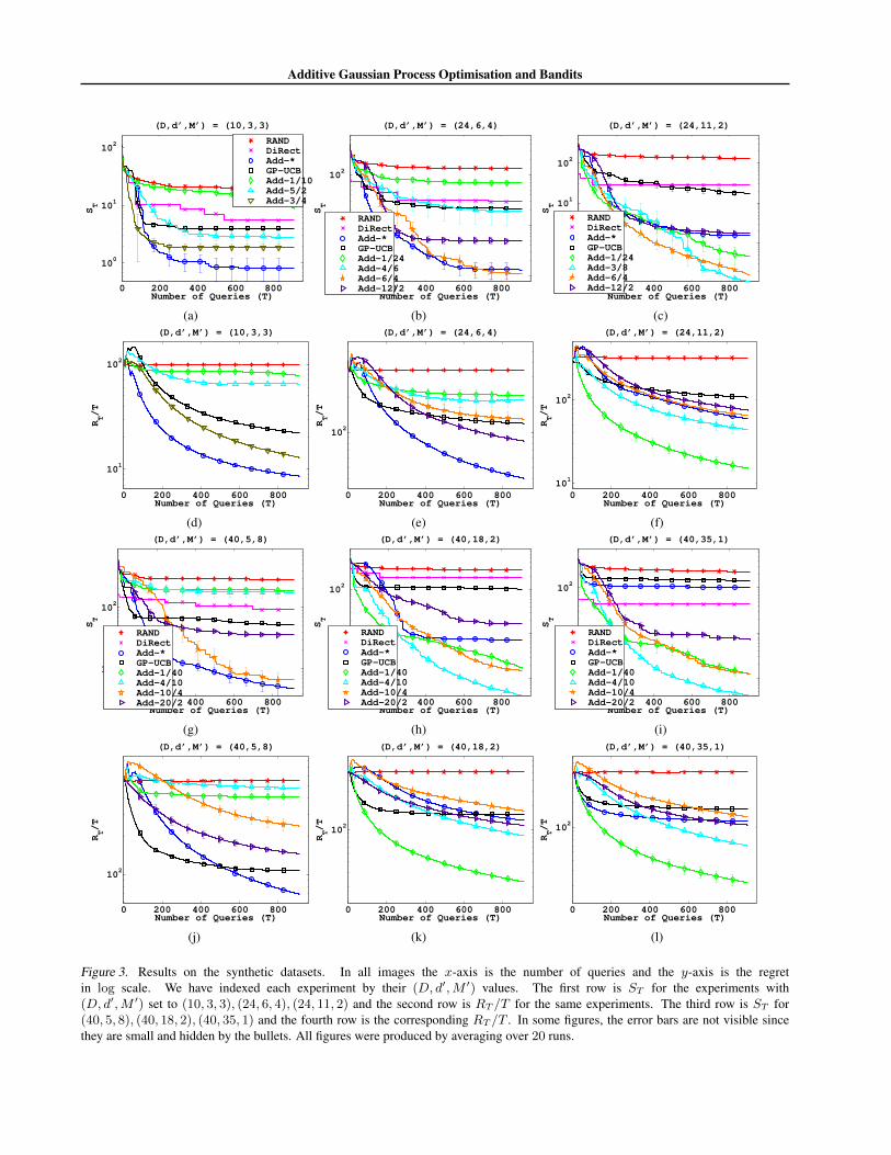
The results are given in Figures 3 and 4. We refer to eachexample by the configuration of the additive function–its(D, d′,M ′) values. In the (10, 3, 3) example Add-? does

4While the 90% seems arbitrary, in our experiments this washardly a factor as the cost was dominated by the inversion of ∆.


0 200 400 600 800

100

101

102

Number of Queries (T)

ST

(D,d’,M’) = (10,3,3)

RANDDiRectAdd−*GP−UCBAdd−1/10Add−5/2Add−3/4

(a)

0 200 400 600 800

100

101

102


ST

(D,d’,M’) = (24,6,4)

RANDDiRectAdd−*GP−UCBAdd−1/24Add−4/6Add−6/4Add−12/2

(b)

0 200 400 600 800

100

101

102


ST

(D,d’,M’) = (24,11,2)


(c)

0 200 400 600 800

101

102

RT/T


(D,d’,M’) = (10,3,3)

(d)

0 200 400 600 800

102

RT/T


(D,d’,M’) = (24,6,4)

(e)

0 200 400 600 800

101

102

RT/T


(D,d’,M’) = (24,11,2)

(f)

0 200 400 600 800

101

102


ST

(D,d’,M’) = (40,5,8)


(g)

0 200 400 600 800

100

101

102


ST

(D,d’,M’) = (40,18,2)


(h)

0 200 400 600 800

100

101

102


ST

(D,d’,M’) = (40,35,1)


(i)

0 200 400 600 800

102

RT/T


(D,d’,M’) = (40,5,8)

(j)

0 200 400 600 800

102

RT/T


(D,d’,M’) = (40,18,2)

(k)

0 200 400 600 800

102

RT/T


(D,d’,M’) = (40,35,1)

(l)

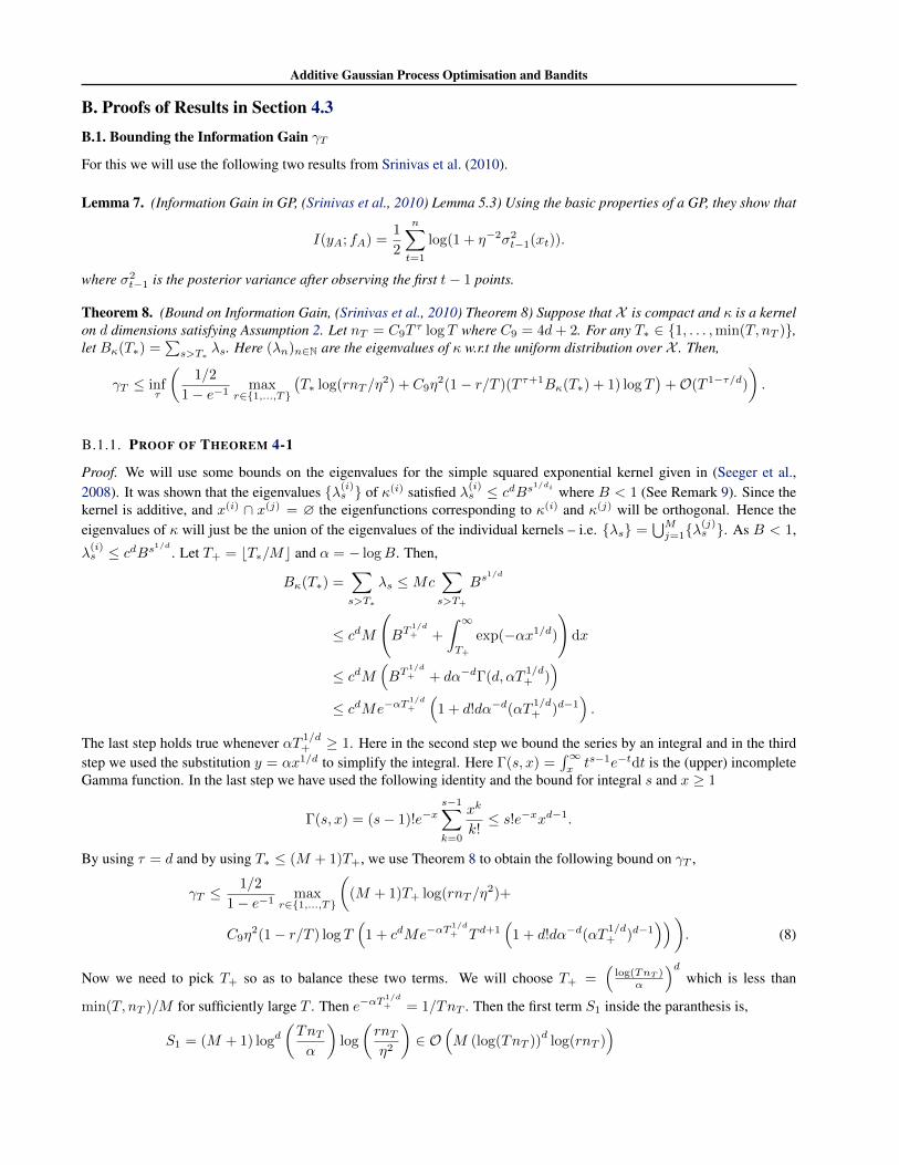
Figure 3. Results on the synthetic datasets. In all images the x-axis is the number of queries and the y-axis is the regretin log scale. We have indexed each experiment by their (D, d′,M ′) values. The first row is ST for the experiments with(D, d′,M ′) set to (10, 3, 3), (24, 6, 4), (24, 11, 2) and the second row is RT /T for the same experiments. The third row is ST for(40, 5, 8), (40, 18, 2), (40, 35, 1) and the fourth row is the corresponding RT /T . In some figures, the error bars are not visible sincethey are small and hidden by the bullets. All figures were produced by averaging over 20 runs.


0 200 400 600 800

102

103


ST

(D,d’,M’) = (96,5,19)


(a)

0 200 400 600 800

101

102

103


ST

(D,d’,M’) = (96,29,3)


(b)

0 200 400 600 800

102

103


ST

(D,d’,M’) = (120,55,2)


(c)

0 200 400 600 800

103

RT/T


(D,d’,M’) = (96,5,19)

(d)

0 200 400 600 800

103

RT/T


(D,d’,M’) = (96,29,3)

(e)

0 200 400 600 800

103

RT/T


(D,d’,M’) = (120,55,2)

(f)

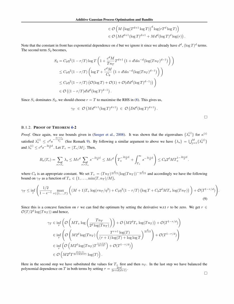
Figure 4. More results on synthetic experiments. The simple regret ST (first row) and cumulative regret RT /T (second row) forfunctions with (D, d′,M ′) set to (96, 5, 19), (96, 29, 3), (120, 55, 2) respectively. Read the caption under Figure 3 for more details.

best since it knows the correct model and the acquisitionfunction can be maximised within the budget. HoweverAdd-3/4 and Add-5/2 models do well too and outperformGP-UCB. Add-1/10 performs poorly since it is statisti-cally not expressive enough to capture the true function.In the (24, 11, 2), (40, 18, 2), (40, 35, 1), (96, 29, 3) and(120, 55, 2) examples Add-? outperforms GP-UCB. How-ever, it is not competitive with the Add-d/M for small d.Even though Add-? knew the correct decomposition, thereare two possible failure modes since d′ is large. The kernelis complex and the estimation error is very high in the ab-sence of sufficient data points. In addition, optimising theacquisition is also difficult. This illustrates our previous ar-gument that using an additive kernel can be advantageouseven if the function is not additive or the decomposition isnot known. In the (24, 6, 4), (40, 5, 8) and (96, 5, 19) ex-amples Add-? performs best as d′ is small enough. Butagain, almost all Add-d/M instantiations outperform GP-UCB. In contrast to the small D examples, for large D,GP-UCB and Add-d/M with large d perform worse thanDiRect. This is probably because our budget for maximis-ing ϕt is inadequate to optimise the acquisition functionto sufficient accuracy. For some of the large D examplesthe cumulative regret is low for Add-GP-UCB and Add-d/M with large d. This is probably since they have al-ready started exploiting where as the Add-d/M with small

d methods are still exploring. We posit that if we run formore iterations we will be able to see the improvements.

5.2. SDSS Astrophysical Dataset

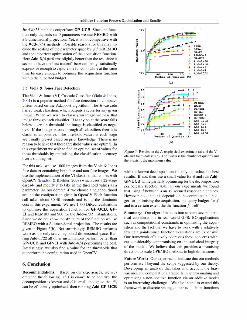
Here we used Galaxy data from the Sloan Digital Sky Sur-vey (SDSS). The task is to find the maximum likelihoodestimators for a simulation based astrophysical likelihoodmodel. Data and software for computing the likelihood aretaken from Tegmark et al (2006). The software itself takesin only 9 parameters but we augment this to 20 dimensionsto emulate the fact that in practical astrophysical problemswe may not know the true parameters on which the prob-lem is dependent. This also allows us to effectively demon-strate the superiority of our methods over alternatives. Eachquery to this likelihood function takes about 2-5 seconds.In order to be wall clock time competitive with RAND andDiRectwe use only 500 evaluations for GP-UCB, GP-EIand REMBO and 450 for Add-d/M to maximise the ac-quisition function.

We have shown the Maximum value obtained over 400 it-erations of each algorithm in Figure 5(a). Note that RANDoutperforms DiRect here since a random query strategyis effectively searching in 9 dimensions. Despite this ad-vantage to RAND all BO methods do better. Moreover,despite the fact that the function may not be additive, all


Add-d/M methods outperform GP-UCB. Since the func-tion only depends on 9 parameters we use REMBO witha 9 dimensional projection. Yet, it is not competitive withthe Add-d/M methods. Possible reasons for this may in-clude the scaling of the parameter space by

√d in REMBO

and the imperfect optimisation of the acquisition function.Here Add-5/4 performs slightly better than the rest since itseems to have the best tradeoff between being statisticallyexpressive enough to capture the function while at the sametime be easy enough to optimise the acquisition functionwithin the allocated budget.

5.3. Viola & Jones Face Detection

The Viola & Jones (VJ) Cascade Classifier (Viola & Jones,2001) is a popular method for face detection in computervision based on the Adaboost algorithm. The K-cascadehas K weak classifiers which outputs a score for any givenimage. When we wish to classify an image we pass thatimage through each classifier. If at any point the score fallsbelow a certain threshold the image is classified as nega-tive. If the image passes through all classifiers then it isclassified as positive. The threshold values at each stageare usually pre-set based on prior knowledge. There is noreason to believe that these threshold values are optimal. Inthis experiment we wish to find an optimal set of values forthese thresholds by optimising the classification accuracyover a training set.

For this task, we use 1000 images from the Viola & Jonesface dataset containing both face and non-face images. Weuse the implementation of the VJ classifier that comes withOpenCV (Bradski & Kaehler, 2008) which uses a 22-stagecascade and modify it to take in the threshold values as aparameter. As our domain X we choose a neighbourhoodaround the configuration given in OpenCV. Each functioncall takes about 30-40 seconds and is the the dominantcost in this experiment. We use 1000 DiRect evaluationsto optimise the acquisition function for GP-UCB, GP-EI and REMBO and 900 for the Add-d/M instantiations.Since we do not know the structure of the function we useREMBO with a 5 dimensional projection. The results aregiven in Figure 5(b). Not surprisingly, REMBO performsworst as it is only searching on a 5 dimensional space. Bar-ring Add-1/22 all other instantiations perform better thanGP-UCB and GP-EI with Add-6/4 performing the best.Interestingly, we also find a value for the thresholds thatoutperform the configuration used in OpenCV.

6. ConclusionRecommendations: Based on our experiences, we rec-ommend the following. If f is known to be additive, thedecomposition is known and d is small enough so that ϕtcan be efficiently optimised, then running Add-GP-UCB

0 100 200 300 400−10

3

−102

−101


Maximum Value

RANDDiRectGP−EIREMBO−9GP−UCBAdd−1/20Add−2/10Add−4/5Add−5/4Add−10/2

(a)

0 100 200 300

65

70

75

80

85

90

95

Number of Queries (T)Classification Accuracy

OpenCVRANDDiRectGP−EIREMBO−5GP−UCBAdd−1/22Add−4/6Add−6/4Add−8/3Add−11/2

(b)

Figure 5. Results on the Astrophysical experiment (a) and the Vi-ola and Jones dataset (b). The x-axis is the number of queries andthe y-axis is the maximum value.

with the known decomposition is likely to produce the bestresults. If not, then use a small value for d and run Add-GP-UCB while partially optimising for the decompositionperiodically (Section 4.4). In our experiments we foundthat using d between 3 an 12 seemed reasonable choices.However, note that this depends on the computational bud-get for optimising the acquisition, the query budget for fand to a certain extent the the function f itself.

Summary: Our algorithm takes into account several prac-tical considerations in real world GPB/ BO applicationssuch as computational constraints in optimising the acqui-sition and the fact that we have to work with a relativelyfew data points since function evaluations are expensive.Our framework effectively addresses these concerns with-out considerably compromising on the statistical integrityof the model. We believe that this provides a promisingdirection to scale GPB/ BO methods to high dimensions.

Future Work: Our experiments indicate that our methodsperform well beyond the scope suggested by our theory.Developing an analysis that takes into account the bias-variance and computational tradeoffs in approximating andoptimising a non-additive function via an additive modelis an interesting challenge. We also intend to extend thisframework to discrete settings, other acquisition functions


and handle more general decompositions.

AcknowledgementsWe wish to thank Akshay Krishnamurthy and AndrewGordon Wilson for the insightful discussions and AndreasKrause, Sham Kakade and Matthias Seeger for the help-ful email conversations. This research is partly funded byDOE grant DESC0011114.

Our current analysis, specifically equation 14, has an error.We are working on resolving this and will post an updateshortly. We would like to thank Felix Berkenkamp and An-dreas Krause from ETH Zurich for pointing this out.

ReferencesAuer, Peter. Using Confidence Bounds for Exploitation-

exploration Trade-offs. J. Mach. Learn. Res., 2003.

Azimi, Javad, Fern, Alan, and Fern, Xiaoli Z. BatchBayesian Optimization via Simulation Matching. In Ad-vances in Neural Information Processing Systems, 2010.

Bergstra, James S., Bardenet, Remi, Bengio, Yoshua, andKegl, Balazs. Algorithms for Hyper-Parameter Opti-mization. In Advances in Neural Information ProcessingSystems, 2011.

Bradski, Gary and Kaehler, Adrian. Learning OpenCV.O’Reilly Media Inc., 2008.

Brochu, Eric, Cora, Vlad M., and de Freitas, Nando. ATutorial on Bayesian Optimization of Expensive CostFunctions, with Application to Active User Modelingand Hierarchical Reinforcement Learning. CoRR, 2010.

Bull, Adam D. Convergence Rates of Efficient Global Op-timization Algorithms. Journal of Machine Learning Re-search, 2011.

Chen, Bo, Castro, Rui, and Krause, Andreas. Joint Op-timization and Variable Selection of High-dimensionalGaussian Processes. In Int’l Conference on MachineLearning, 2012.

de Freitas, Nando. Talk on Current Challenges and OpenProblems in Bayesian Optimization, 2014.

de Freitas, Nando, Smola, Alex J., and Zoghi, Masrour.Exponential Regret Bounds for Gaussian Process Ban-dits with Deterministic Observations. In InternationalConference on Machine Learning, 2012.

Denil, Misha, Bazzani, Loris, Larochelle, Hugo, andde Freitas, Nando. Learning Where to Attend withDeep Architectures for Image Tracking. Neural Com-put., 2012.

Djolonga, Josip, Krause, Andreas, and Cevher, Volkan.High-Dimensional Gaussian Process Bandits. In Ad-vances in Neural Information Processing Systems, 2013.

Duvenaud, David K., Nickisch, Hannes, and Rasmussen,Carl Edward. Additive gaussian processes. In Advancesin Neural Information Processing Systems, 2011.

Ghosal, Subhashis and Roy, Anindya. Posterior consis-tency of Gaussian process prior for nonparametric binaryregression”. Annals of Statistics, 2006.

Gonzalez, Javier, Longworth, Joseph, James, David, andLawrence, Neil. Bayesian Optimization for SyntheticGene Design. In NIPS Workshop on Bayesian Optimiza-tion in Academia and Industry, 2014.

Gyorfi, Laszlo, Kohler, Micael, Krzyzak, Adam, and Walk,Harro. A Distribution Free Theory of Nonparametric Re-gression. Springer Series in Statistics, 2002.

Hastie, T. J. and Tibshirani, R. J. Generalized AdditiveModels. London: Chapman & Hall, 1990.

Hoffman, Matthew D., Brochu, Eric, and de Freitas,Nando. Portfolio Allocation for Bayesian Optimization.In Uncertainty in Artificial Intelligence, 2011.

Hornby, G. S., Globus, A., Linden, D.S., and Lohn, J.D.Automated Antenna Design with Evolutionary Algo-rithms. American Institute of Aeronautics and Astronau-tics, 2006.

Jones, D. R., Perttunen, C. D., and Stuckman, B. E. Lips-chitzian Optimization Without the Lipschitz Constant. J.Optim. Theory Appl., 1993.

Jones, Donald R., Schonlau, Matthias, and Welch,William J. Efficient global optimization of expensiveblack-box functions. J. of Global Optimization, 1998.

Kandasamy, Kirthevasan, Schneider, Jeff, and Poczos,Barnabas. Bayesian Active Learning for Posterior Es-timation. In International Joint Conference on ArtificialIntelligence, 2015.

Lizotte, Daniel, Wang, Tao, Bowling, Michael, and Schuur-mans, Dale. Automatic gait optimization with gaussianprocess regression. In in Proc. of IJCAI, pp. 944–949,2007.

Ma, Yifei, Sutherland, Dougal J., Garnett, Roman, andSchneider, Jeff G. Active Pointillistic Pattern Search. InInternational Conference on Artificial Intelligence andStatistics, AISTATS, 2015.

Mahendran, Nimalan, Wang, Ziyu, Hamze, Firas, andde Freitas, Nando. Adaptive MCMC with Bayesian Op-timization. In Artificial Intelligence and Statistics, 2012.


Martinez-Cantin, R., de Freitas, N., Doucet, A., and Castel-lanos, J. Active Policy Learning for Robot Planningand Exploration under Uncertainty. In Proceedings ofRobotics: Science and Systems, 2007.

Mockus, J.B. and Mockus, L.J. Bayesian approach toglobal optimization and application to multiobjectiveand constrained problems. Journal of Optimization The-ory and Applications, 1991.

Mockus, Jonas. Application of Bayesian approach to nu-merical methods of global and stochastic optimization.Journal of Global Optimization, 1994.

Osborne, M., Duvenaud, D., Garnett, R., Rasmussen, C.,Roberts, S., and Ghahramani, Z. Active Learning ofModel Evidence Using Bayesian Quadrature. In NeuralInformation Processing Systems (NIPS), 2012.

Parkinson, David, Mukherjee, Pia, and Liddle, Andrew R.A Bayesian model selection analysis of WMAP3. Phys-ical Review, 2006.

Rasmussen, C.E. and Williams, C.K.I. Gaussian Processesfor Machine Learning. Adaptative computation and ma-chine learning series. University Press Group Limited,2006.

Ravikumar, Pradeep, Lafferty, John, Liu, Han, and Wasser-man, Larry. Sparse Additive Models. Journal of theRoyal Statistical Society: Series B (Statistical Method-ology), 2009.

Seeger, MW., Kakade, SM., and Foster, DP. InformationConsistency of Nonparametric Gaussian Process Meth-ods. IEEE Transactions on Information Theory, 2008.

Snoek, Jasper, Larochelle, Hugo, and Adams, Ryan P.Practical Bayesian Optimization of Machine LearningAlgorithms. In Advances in Neural Information Process-ing Systems, 2012.

Srinivas, Niranjan, Krause, Andreas, Kakade, Sham, andSeeger, Matthias. Gaussian Process Optimization in theBandit Setting: No Regret and Experimental Design. InInternational Conference on Machine Learning, 2010.

Tegmark et al, M. Cosmological Constraints from theSDSS Luminous Red Galaxies. Physical Review, De-cember 2006.

Thompson, W. R. On the Likelihood that one UnknownProbability Exceeds Another in View of the Evidence ofTwo Samples. Biometrika, 1933.

Viola, Paul A. and Jones, Michael J. Rapid Object De-tection using a Boosted Cascade of Simple Features. InComputer Vision and Pattern Recognition, 2001.

Wang, Ziyu, Zoghi, Masrour, Hutter, Frank, Matheson,David, and de Freitas, Nando. Bayesian Optimization inHigh Dimensions via Random Embeddings. In Interna-tional Joint Conference on Artificial Intelligence, 2013.

Yamins, Daniel, Tax, David, and Bergstra, James S. Mak-ing a Science of Model Search: Hyperparameter Opti-mization in Hundreds of Dimensions for Vision Archi-tectures. In International Conference on Machine Learn-ing, 2013.


A. Some Auxiliary MaterialA.1. Review of the GP-UCB Algorithm

In this subsection we present a brief summary of the GP-UCB algorithm in (Srinivas et al., 2010). The algorithm is givenin Algorithm 3.

The following theorem gives the rate of convergence for GP-UCB. Note that under an additive kernel, this is the samerate as Theorem 5 which uses a different acquisition function. Note the differences in the choice of βt.

Theorem 6. (Modification of Theorem 2 in (Srinivas et al., 2010)) Suppose f is constructed by sampling f (j) ∼GP(0, κ(j)) for j = 1, . . . ,M and then adding them. Let all kernels κ(j) satisfy assumption 2 for some L, a, b. Fur-ther, we maximise the acquisition function ϕt to within ζ0t−1/2 accuracy at time step t. Pick δ ∈ (0, 1) and choose

βt = 2 log

(2t2π2

δ

)+ 2D log

(Dt3

)∈ O (D log t) .

Then, GP-UCB attains cumulative regretRT ∈ O(√

DγTT log T)

and hence simple regret ST ∈ O(√

DγT log T/T)

.Precisely, with probability > 1− δ,

∀T ≥ 1, RT ≤√

8C1βTMTγt + 2ζ0√T + C2.

where C1 = 1/ log(1 + η−2) and C2 is a constant depending on a, b, D, δ, L and η.

Proof. Srinivas et al. (2010) bound the regret for exact maximisation of the GP-UCB acquisition ϕt. By following ananalysis similar to our proof of Theorem 5 the regret can be shown to be the same for an ζ0t−1/2- optimal maximisation.

Algorithm 3 GP-UCBInput: Kernel κ, Input Space X .For t = 1, 2 . . .• D0 ← ∅,• (µ0, κ0)← (0, κ)• for t = 1, 2, . . .

1. xt ← argmaxz∈X µt−1(z) +√βtσt−1(z)

2. yt ← Query f at xt.3. Dt = Dt−1 ∪ (xt,yt).4. Perform Bayesian posterior updates to obtain µt, σt for j = 1, . . . ,M .

A.2. Sequential Optimisation Approaches

If the function is known to be additive, we could consider several other approaches for maximisation. We list two of themhere and explain their deficiencies. We recommend that the reader read the main text before reading this section.

A.2.1. OPTIMISE ONE GROUP AND PROCEED TO THE NEXT

First, fix the coordinates of x(j), j 6= 1 and optimise w.r.t x(1) by querying the function for a pre-specified number of times.Then we proceed sequentially optimising with respect to x(2), x(3) . . . . We have outlined this algorithm in Algorithm 4.There are several reasons this approach is not desirable.

• First, it places too much faith on the additive assumption and requires that we know the decomposition at the startof the algorithm. Note that this strategy will only have searched the space in M d-dimensional subspaces. In ourapproach even if the function is not additive we can still hope to do well since we learn the best additive approximationto the true function. Further, if the decomposition is not known we could learn the decomposition “on the go” or atleast find a reasonably good decomposition as we have explained in Section 4.4.


• Such a sequential approach is not an anytime algorithm. This in particular means that we need to predetermine thenumber of queries to be allocated to each group. After we proceed to a new group it is not straightforward to comeback and improve on the solution obtained for an older group.

• This approach is not suitable for the bandits setting. We suffer large instantaneous regret up until we get to the lastgroup. Further, after we proceed beyond a group since we cannot come back, we cannot improve on the best regretobtained in that group.

Our approach does not have any of these deficiencies.

Algorithm 4 Seq-Add-GP-UCBInput: Kernels κ(1), . . . , κ(M), Decomposition (X (j))Mj=1, Query Budget T ,• RD 3 θ =

⋃Mj=1 θ

(j) = rand([0, 1]d)• for j = 1, . . . ,M

1. D(j)0 ← ∅,

2. (µ(j)0 , κ

(j)0 )← (0, κ(j)).

3. for t = 1, 2, . . . T/M

(a) x(j)t ← argmaxz∈X (j) µ(j)(z) +

√βtσ

(j)(z)

(b) xt ← x(j)t

⋃k 6=j θ

(k).(c) yt ← Query f at xt.(d) D(j)

t = D(j)t−1 ∪ (x

(j)t ,yt).

(e) Perform Bayesian posterior updates to obtain µ(j)t , σ

(j)t .

4. θ(j) ← x(j)T/M

• Return θ

A.2.2. ONLY CHANGE ONE GROUP PER QUERY

In this strategy, the approach would be very similar to Add-GP-UCB except that at each query we will only update onegroup at time. If it is the kth group the query point is determined by maximising ϕ(k)

t for x(k)t and for all other groups we use

values from the previous rotation. After M iterations we cycle through the groups. We have outlined this in Algorithm 5.

This is a reasonable approach and does not suffer from the same deficiencies as Algorithm 4. Maximising the acquisitionfunction will also be slightly easier O(ζ−d) since we need to optimise only one group at a time. However, the regret forthis approach would beO(M

√DγTT log T ) which is a factor ofM worse than the regret in our method (This can be show

by following an analysis similar to the one in section B.2. This is not surprising, since at each iteration you are moving ind-coordinates of the space and you have to wait M iterations before the entire point is updated.

Algorithm 5 Add-GP-UCB-BuggyInput: Kernels κ(1), . . . , κ(M), Decomposition (X (j))Mj=1

• D0 ← ∅,• for j = 1, . . . ,M , (µ

(j)0 , κ

(j)0 )← (0, κ(j)).

• for t = 1, 2, . . .

1. k = j mod M

2. x(k)t ← argmaxz∈X (k) µ(k)(z) +

√βtσ

(k)(z)

3. for j 6= k, x(j)t ← x

(j)t−1

4. xt ←⋃Mj=1 x

(j)t .

5. yt ← Query f at xt.6. Dt = Dt−1 ∪ (xt,yt).7. Perform Bayesian posterior updates to obtain µ(j)

t , σ(j)t for j = 1, . . . ,M .


B. Proofs of Results in Section 4.3B.1. Bounding the Information Gain γT

For this we will use the following two results from Srinivas et al. (2010).

Lemma 7. (Information Gain in GP, (Srinivas et al., 2010) Lemma 5.3) Using the basic properties of a GP, they show that

I(yA; fA) =1

2

n∑t=1

log(1 + η−2σ2t−1(xt)).

where σ2t−1 is the posterior variance after observing the first t− 1 points.

Theorem 8. (Bound on Information Gain, (Srinivas et al., 2010) Theorem 8) Suppose that X is compact and κ is a kernelon d dimensions satisfying Assumption 2. Let nT = C9T

τ log T where C9 = 4d+ 2. For any T∗ ∈ 1, . . . ,min(T, nT ),let Bκ(T∗) =

∑s>T∗

λs. Here (λn)n∈N are the eigenvalues of κ w.r.t the uniform distribution over X . Then,

γT ≤ infτ

(1/2

1− e−1max

r∈1,...,T

(T∗ log(rnT /η

2) + C9η2(1− r/T )(T τ+1Bκ(T∗) + 1) log T

)+O(T 1−τ/d)

).

B.1.1. PROOF OF THEOREM 4-1

Proof. We will use some bounds on the eigenvalues for the simple squared exponential kernel given in (Seeger et al.,2008). It was shown that the eigenvalues λ(i)

s of κ(i) satisfied λ(i)s ≤ cdBs

1/di where B < 1 (See Remark 9). Since thekernel is additive, and x(i) ∩ x(j) = ∅ the eigenfunctions corresponding to κ(i) and κ(j) will be orthogonal. Hence theeigenvalues of κ will just be the union of the eigenvalues of the individual kernels – i.e. λs =

⋃Mj=1λ

(j)s . As B < 1,

λ(i)s ≤ cdBs

1/d

. Let T+ = bT∗/Mc and α = − logB. Then,

Bκ(T∗) =∑s>T∗

λs ≤Mc∑s>T+

Bs1/d

≤ cdM

(BT

1/d+ +

∫ ∞T+

exp(−αx1/d)

)dx

≤ cdM(BT

1/d+ + dα−dΓ(d, αT

1/d+ )

)≤ cdMe−αT

1/d+

(1 + d!dα−d(αT

1/d+ )d−1

).

The last step holds true whenever αT 1/d+ ≥ 1. Here in the second step we bound the series by an integral and in the third

step we used the substitution y = αx1/d to simplify the integral. Here Γ(s, x) =∫∞xts−1e−tdt is the (upper) incomplete

Gamma function. In the last step we have used the following identity and the bound for integral s and x ≥ 1

Γ(s, x) = (s− 1)!e−xs−1∑k=0

xk

k!≤ s!e−xxd−1.

By using τ = d and by using T∗ ≤ (M + 1)T+, we use Theorem 8 to obtain the following bound on γT ,

γT ≤1/2

1− e−1max

r∈1,...,T

((M + 1)T+ log(rnT /η

2)+

C9η2(1− r/T ) log T

(1 + cdMe−αT

1/d+ T d+1

(1 + d!dα−d(αT

1/d+ )d−1

))). (8)

Now we need to pick T+ so as to balance these two terms. We will choose T+ =(

log(TnT )α

)dwhich is less than

min(T, nT )/M for sufficiently large T . Then e−αT1/d+ = 1/TnT . Then the first term S1 inside the paranthesis is,

S1 = (M + 1) logd(TnTα

)log

(rnTη2

)∈ O

(M (log(TnT ))

dlog(rnT )

)


∈ O(M(log(T d+1 log T )

)dlog(rT d log T )

)∈ O

(Mdd+1(log T )d+1 +Mdd(log T )d log(r)

).

Note that the constant in front has exponential dependence on d but we ignore it since we already have dd, (log T )d terms.The second term S2 becomes,

S2 = C9η2(1− r/T ) log T

(1 +

cdM

TnTT d+1

(1 + d!dα−d(log(TnT )d−1

)))≤ C9η

2(1− r/T )

(log T +

cdM

C9

(1 + d!dα−d(log(TnT )d−1

)))≤ C9η

2(1− r/T )(O(log T ) +O(1) +O(d!dd(log T )d−1)

))∈ O

((1− r/T )d!dd(log T )d−1

).

Since S1 dominates S2, we should choose r = T to maximise the RHS in (8). This gives us,

γT ∈ O(Mdd+1(log T )d+1

)∈ O

(Ddd(log T )d+1

).

B.1.2. PROOF OF THEOREM 4-2

Proof. Once again, we use bounds given in (Seeger et al., 2008). It was shown that the eigenvalues λ(i)s for κ(i)

satisfied λ(i)s ≤ cds

−2ν+djdj (See Remark 9). By following a similar argument to above we have λs =

⋃Mj=1λ

(j)s

and λ(i)s ≤ cds−

2ν+dd . Let T+ = bT∗/Mc. Then,

Bκ(T∗) =∑s>T∗

λs ≤Mcd∑s>T+

s−2ν+dd ≤Mcd

(T− 2ν+d

d+ +

∫ ∞T+

s−2ν+dd

)≤ C82dMT

1− 2ν+dd

+ .

where C8 is an appropriate constant. We set T+ = (TnT )d

2ν+d (log(TnT ))−d

2ν+d and accordingly we have the followingbound on γT as a function of T+ ∈ 1, . . . ,min(T, nT )/M,

γT ≤ infτ

(1/2

1− e−1max

r∈1,...,T

((M + 1)T+ log(rnT /η

2) + C9η2(1− r/T )

(log T + C82dMT+ log(TnT )

))+O(T 1−τ/d)

).

(9)

Since this is a concave function on r we can find the optimum by setting the derivative w.r.t r to be zero. We get r ∈O(T/2d log(TnT )) and hence,

γT ∈ infτ

(O(MT+ log

(TnT

2d log(TnT )

))+O

(M2dT+ log(TnT )

)+O(T 1−τ/d)

)∈ inf

τ

(O

(M2d log(TnT )

(T τ+1 log(T )

(τ + 1) log(T ) + log log T

) d2ν+d

)+O(T 1−τ/d)

)∈ inf

τ

(O(M2d log(TnT )T

(τ+1)d2ν+d

)+O(T 1−τ/d)

)∈ O

(M2dT

d(d+1)2ν+d(d+1) log(T )

).

Here in the second step we have substituted the values for T+ first and then nT . In the last step we have balanced thepolynomial dependence on T in both terms by setting τ = 2νd

2ν+d(d+1) .


Remark 9. The eigenvalues and eigenfunctions for the kernel are defined with respect to a base distribution on X . Inthe development of Theorem 8, Srinivas et al. (2010) draw nT samples from the uniform distribution on X . Hence, theeigenvalues/eigenfunctions should be w.r.t the uniform distribution. The bounds given in Seeger et al. (2008) are for theuniform distribution for the Matern kernel and a Gaussian Distribution for the Squared Exponential Kernel. For the lattercase, Srinivas et al. (2010) argue that the uniform distribution still satisfies the required tail constraints and therefore thebounds would only differ up to constants.

B.2. Rates on Add-GP-UCB

Our analysis in this section draws ideas from Srinivas et al. (2010). We will try our best to stick to their same notation.However, unlike them we also handle the case where the acquisition function is optimised within some error. In theensuing discussion, we will use xt =

⋃j x

(j)t to denote the true maximiser of ϕt – i.e. x

(j)t = argmaxz∈X (j) ϕ

(j)t (z).

xt =⋃j x

(j)t denotes the point chosen by Add-GP-UCB at the tth iteration. Recall that xt is ζ0t−1/2–optimal; I.e.

ϕt(xt)− ϕt(xt) ≤ ζ0t−1/2.

Denote p =∑j dj . πt denotes a sequence such that

∑t π−1t = 1. For e.g. when we use πt = π2t2/6 below, we obtain

the rates in Theorem 5.

In what follows, we will construct discretisations Ω(j) on each group X (j) for the sake of analysis. Letωj = |Ω(j)| and ωm = maxj ωj . The discretisation of the individual groups induces a discretisation Ω on X it-self, Ω = x =

⋃j x

(j) : x(j) ∈ Ω(j), j = 1, . . . ,M. Let ω = |Ω| =∏j ωj . We first establish the following two lemmas

before we prove Theorem 5.

Lemma 10. Pick δ ∈ (0, 1) and set βt = 2 log(ωmMπt/δ). Then with probability > 1− δ,

∀t ≥ 1,∀x ∈ Ω, |f(x)− µt−1(x)| ≤ β1/2t

M∑j=1

σ(j)t−1(x(j)).

Proof. Conditioned on Dt−1, at any given x and t we have f(x(j)) ∼ N (µ(j)t−1(x(j)), σ

(j)t−1j), ∀j = 1, . . .M . Using the

tail bound, P(z > M) ≤ 12e−M2/2 for z ∼ N (0, 1) we have with probability > 1− δ/ωMπt,

|f (j)(x(j))− µ(j)t−1(x(j))|

σ(j)t−1(x(j))

> β1/2t ≤ e−βt/2 =

δ

ωmMπt.

By using a union bound ωj ≤ ωm times over all x(j) ∈ Ω(j) and then M times over all discretisations the above holdswith probability > 1 − δ/πt for all j = 1, . . . ,M and x(j) ∈ Ω(j). Therefore, we have |f(x) − µt−1(x)| ≤ |f(x(j)) −µ

(j)t−1(x(j))| ≤ β1/2

t

∑j σ

(j)t−1(x(j)) for all x ∈ Ω. Now using the union bound on all t yields the result.

Lemma 11. The posterior mean µt−1 for a GP whose kernel κ(·, x) is L-Lipschitz satisfies,

P(∀t ≥ 1 |µt−1(x)− µt−1(x′)| ≤

(f(x∗) + η

√2 log(πt/2δ)

)Lη−2t‖x− x′‖2

)≥ 1− δ.

Proof. Note that for given t,

P(yt < f(x∗) + η

√2 log(πt/2δ)

)≤ P

(εt/η <

√2 log(πt/2δ)

)≤ δ/πt.

Therefore the statement is true with probability > 1 − δ for all t. Further, ∆ η2I implies ‖∆−1‖op ≤ η−2 and|k(x, z)− k(x′, z)| ≤ L‖x− x′‖. Therefore

|µt−1(x)− µt−1(x′)| = |Y >t−1∆−1(k(x,XT )− k(x′, XT )| ≤ ‖Yt−1‖2‖∆−1‖op‖k(x,Xt−1)− k(x′, Xt−1)‖2

≤(f(x∗) + η

√2 log(πt/2δ)

)Lη−2(t− 1)‖x− x′‖2.


B.2.1. PROOF OF THEOREM 5

Proof. First note that by Assumption 2 and the union bound we have, P(∀i supx(j)∈X (j) |∂f (j)(x(j))/∂x(j)i | > J) ≤

diae−(J/b)2 . Since, ∂f(x)/∂x

(j)i = ∂f (j)(x(j))/∂x

(j)i , we have,

P(∀i = 1, . . . , D sup

x∈X

∣∣∣∂f(x)

∂xi

∣∣∣ > J

)≤ pae−(J/b)2 .

By setting δ/3 = pae−J2/b2 we have with probability > 1− δ/3,

∀x, x′ ∈ X , |f(x)− f(x′)| ≤ b√

log(3ap/δ)‖x− x′‖1. (10)

Now, we construct a sequence of discretisations Ω(j)t satisfying ‖x(j) − [x(j)]t]‖1 ≤ dj/τt ∀x(j) ∈ Ω

(j)t . Here, [x(j)]t is

the closest point to x(j) in Ω(j)t in an L2 sense. A sufficient discretisation is a grid with τt uniformly spaced points. Then

it follows that for all x ∈ Ωt, ‖x − [x]t‖1 ≤ p/τt. Here Ωt is the discretisation induced on X by the Ω(j)t ’s and [x]t is

the closest point to x in Ωt. Note that ‖x(j) − [x(j)]t‖2 ≤√dj/τt ∀x(j) ∈ Ω(j) and ‖x − [x]t‖2 ≤

√p/τt. We will

set τt = pt3–therefore, ωtj ≤ (pt3)d∆= ωmt. When combining this with (10), we get that with probability > 1 − δ/3,

|f(x)− f([x])| ≤ b√

log(3ap/δ)/t3. By our choice of βt and using Lemma 10 the following is true for all t ≥ 1 and forall x ∈ X with probability > 1− 2δ/3,

|f(x)− µt−1([x]t)| ≤ |f(x)− f([x]t)|+ |f([x]t)− µt−1([x]t)| ≤b√

log(3ap/δ)

t2+ β

1/2t

M∑j=1

σ(j)t−1([x(j)]t). (11)

By Lemma 11 with probability > 1− δ/3 we have,

∀x ∈ X , |µt−1(x)− µt−1([x]t)| ≤L(f(x∗) + η

√2 log(3πt/2δ)

)√pη2t2

. (12)

We use the above results to obtain the following bound on the instantaneous regret rt which holds with probability > 1− δfor all t ≥ 1,

rt = f(x∗)− f(xt)

≤ µt−1([x∗]t) + β1/2t

M∑j=1

σ(j)t−1([x

(j)∗ ]t)− µt−1([xt]t) + β

1/2t

M∑j=1

σ(j)t−1([x

(j)t ]t) +

2b√

log(3ap/δ)

t3

≤2b√

log(3ap/δ)

t3+ζ0√t

+ β1/2t

M∑j=1

σ(j)t−1(x

(j)t ) +

M∑j=1

σ(j)t−1([x

(j)t ]t)

+ µt−1(xt)− µt−1([xt]t)

≤2b√

log(3ap/δ)

t3+L(f(x∗) + η

√2 log(πt/2δ)

)√pη2t2

+ζ0√t

+ β1/2t

M∑j=1

σ(j)t−1(x

(j)t ) +

M∑j=1

σ(j)t−1([x

(j)t ]t)

. (13)

In the first step we have applied Equation (11) at x∗ and xt. In the second step we have used the fact that ϕt([x∗]t) ≤ϕt(xt) ≤ ϕt(xt) + ζ0t

−1/2. In the third step we have used Equation (12).

For any x ∈ X we can bound σt(x)2 as follows,

σt(x)2

= η2η−2σt(x)2 ≤ 1

log(1 + η−2)log(

1 + η−2σt(x)2).

Here we have used the fact that u2 ≤ v2 log(1 + u2)/ log(1 + v2) for u ≤ v and σt(x)2 ≤ κ(x, x) = 1. Write

C1 = log−1(1 + η−2). By using Jensen’s inequality and Definition 3 for any set of T points x1, x2, . . . xT ⊂ X , T∑t=1

M∑j=1

σ(j)t (x(j))

2

≤MT

T∑t=1

M∑j=1

σ(j)t (x(j))

2≤ C1MT

T∑t=1

log(

1 + η−2σt(x)2)≤ 2C1MTγT . (14)


Finally we can bound the cumulative regret with probability > 1− δ for all T ≥ 1 by,

RT =

T∑t=1

rt ≤ C2(a, b,D, L, δ) + ζ0

T∑t=1

t−1/2 + β1/2T

T∑t=1

M∑j=1

σ(j)t−1(x

(j)t ) +

T∑t=1

M∑j=1

σ(j)t−1([x

(j)t ]t)

≤ C2(a, b,D, L, δ) + 2ζ0

√T +

√8C1βTMTγT .

where we have used the summability of the first two terms in Equation (13). Here, for δ < 0.8, the constant C2 is given by,

C2 ≥ b√

log(3ap/δ) +π2Lf(x∗)

6√pη2

+Lπ3/2

√12pδη

.

Documents

High Dimensional Bayesian Optimisation and Bandits via ...kkandasa/pubs/kandasamyICML15addGPUCB.pdf · High Dimensional Bayesian Optimisation and Bandits via Additive Models Kirthevasan